Submitted:
27 February 2025
Posted:
28 February 2025
You are already at the latest version
Abstract
The values of a measured, derived or estimated variable often differ from the “true”, “undistorted” values of a desired dimension. Output values of non-calibrated measuring instruments, misspecification of analysis models or too inflexible activation functions can lead to inappropriate decisions in all situations. Therefore, a highly flexible mathematical function for the isotonic transformation of a variable X of the value space [0-1] to a variable Y of the same value space [0-1] is presented here. With four or six parameters, almost all conceivable function curves can be represented. This allows restrictions of other functions, e.g. linearity or constant curvature, to be overcome.
Keywords:
transmission
; calibration
; scoring
Introduction
The values of a measured, derived or estimated quantity often differ from the “true”, “unbiased” values of a desired dimension. This is the case, for example, with non- or poorly calibrated measuring instruments or test methods, not only in chemistry, physics, biology or technology. According to ISO 11095, calibration is understood as a procedure by which the systematic differences between a “measurement system” and a “reference system” are determined or equalised [4]. Similarly, a risk model that has been created using a logistic function or machine learning, for example, can be mis-calibrated even if it is considered established. This means that the predicted risks do not accurately capture the event rates in a target population.
However, mis-calibrated values can lead to unfavorable wrong decisions. In banking, for example, the granting of loans is linked to internal bank rating procedures with the allocation of borrowers to rating classes. As part of the calibration process, it must be ensured that the assignment is made in such a way that the historically observed default rates of the borrowers in a rating class correspond to the probability of default in this class [1].
In medicine, sufficiently accurate quantification of a disease marker is essential for diagnosis or accurate monitoring of disease burden. Inadequate determination of a disease risk can lead to erroneous decisions regarding disease screening. Thes same applies to a misinterpretation of a score in the interval 0 to 1 as probability [2]. It has been shown that polygenic risk scores (PRS) should be calibrated on a country-specific basis to determine individual breast cancer risk [3].
A related problem is the specification of a problem-adequate activation function of a node in an artificial neural network. This calculates the output of the node on the basis of its individual inputs and, if necessary, weights. Simple activation functions include the smooth version, the ReLU (Rectified Linear Unit) and the GELU (Gaussian Error Linear Units), as well as the sigmoid, tanh (hyperbolic tangent) and softmax functions, as used in some speech recognition models [5,6]. However, one can find countless activation functions in the relevant specialist literature [7]. Depending on the intended use, this could also be used as a calibration or rescaling function.
Many of the conventional calibration functions are a special case of a general, polynomial power transformation:
(1)
If necessary, X can also be replaced by a rank-preserving transformation, e.g., . or [8]. For many practical applications, fitting a simple, linear calibration function (i.e., and ) is sufficient to equalise distortions between the “measurement system” and the “reference system”. The determination of the parameters and is simple [8]. However, if a (measurement) parameter X of the value space [0-1] has to be monotonically transformed to a (reference) parameter Y of the same value space [0-1], equation [1] is unsuitable. Equation [1] does not guarantee that Y will only have values between 0 and 1. Equation [1] also does not allow X values close to 0 to be assigned a or X values close to 1 to be assigned a .
Definition of a Function for Monotonic Transformation
The following four building blocks are required to define a highly flexible mathematical function for the monotonic transformation of a variable X of the value space [0-1] to a variable Y of the same value space [0-1]:
In order to guarantee only values from the value range [0-1] for Y, the property of the sigmoid function, or its inverse, the logit function, can be utilised. These functions allow a continuous variable x to be mapped in an interval [0,1] and vice versa.
logit-funktion: sigmoid-funktion (2a,b)
where x can take values in the range [0-1] and x’ values in the range [-∞ to+∞].
For a variable X with values in the range [0-1], a scale-transformed variable X’‘ can also be generated with a value range [0-1] by simply exponentiating Finally, a variable X with values in the value range can be proportionally transformed into a variable X’‘‘ in the value range using the following equation:
(3)
If the target variable is to have a value range of [0-1], but the output variable X is to have a flexibly defined value range , the above equation is reduced to:
(3a)
whereas: for ist and for ist .
Conversely, if the output variable X is to have a value range of [0-1], but the target variable is to have a flexibly defined value range , the above equation is reduced to:
(3b)
These four building blocks are now applied step by step to obtain a calibration function :
Step I) Transferring X (value range ) to the value range [0,1]: with u and o boundary parameters
Step II) Rescaling of : with c a scaling parameter
Step III) Transferring (value range [0-1]) to a continuous variable:
Step V) Considering a linear relationship between the calibrated output Y of (value range [0-1]) and the continuous input variable , according to logistics regression:
.
with a as shift parameter and b as slope parameter
Step VI) Inverting this linear relationship according to the sigmoid function:
Step VII) Rescaling of : with d a scaling parameter
This ultimately results in the desired calibration function:
(4)
with and .
Step VII) Rescaling of to One more step can be taken to relax the transformation form the basic requirement of and , to and . This step is optional and should only be used if necessary. Applying equation 3b results in:
(5)
This flexible, limited, double-sigmoid transmission function (FLDSf, equation 5) looks rather complicated, but follows a stringent logic and enables a highly flexible univariate transformation.
However, the parameters a, b, c, d, u and o are subject to the following necessary or sensible restrictions:
Examples of Semi-Flexible Functions
The FLDS function defined above is highly flexible in the form of the “translation” from x to y. The choice of suitable parameters is decisive for the form. Some examples are listed here (Figure 1), whereby the boundary parameters are always fixed to u=0 and o=1.
“linear course”: To obtain a linear curve (y=x), a=0 and b=1 must be selected and c=d must be set.
“concave course”: A concave curve is obtained if the parameter a is increased starting from the linear curve (e.g., a=2).
“convex course”: A concave curve is obtained if, starting from the linear curve, the parameter a is reduced below zero (e.g., a=-2).
“S-shaped course”: An S-shaped curve is obtained if the parameter b is increased from the linear curve (e.g., b=3). The S-shape can be modified with the parameters a, c and d.
“rapidly increasing course”: To obtain a rapidly rising curve, a high value (b=5 and d=3.6) can be selected for b and d and a lower value (e.g., c=0.57) for c. The higher the parameter value for a, the steeper the rise.
The function can be visualized remotely online using the following link: https://www.desmos.com/calculator/ib3yikhfoq?lang=de.
Discussion
The function presented here looks complicated at first glance, but follows a stringent logic and enables an extremely flexible, univariate transformation. It was developed to derive genotype probabilities (naturally restricted to the value space [0-1]) from genotype doses (scaled in the value space [0-1]) determined in a biological experiment. However, the function is universal and can therefore also be used for other purposes. It could conceivably be used to calibrate risk scores or as an activation function in neural networks. The function parameters can be completely or partially set or restricted in order to limit the space or the form of possible function progressions. However, they can also be estimated from data using all known methods (maximum likelihood, minimum loss, grid search, etc.).
Alternatively to the FLDSf, one may apply spline functions or eEmax models. [8,9] Splines are flexible polynomial functions that run piecewise between predefined nodes. They have a reputation for being able to map any curve in a purely data-oriented way, i.e., without assumptions (e.g., linearity). However, this is only true to a limited extent. The complexity of spline functions depends heavily on the number of nodes and the type of degree of the piecewise polynomials. Sigmoid eEmax functions have been shown to be effective in modeling a wider range of concentration-response behavior in pharmacokinetics, including non-sigmoidal patterns. It is considered a robust and flexible method for analyzing drug concentration and effect. However, it is not possible to create an S-shaped curve with the eEmax function. In summary, it can be said that the two alternative functions discussed require fewer parameters than FLDSf, but they also offer a smaller selection of function curves.
Conclusion
The FLDSf function presented here offers a highly flexible way of translating an input variable X from the value range [0-1] into an output variable y in the same value range [0-1]. All or some of the parameters a, b, c, d, u and o can be estimated based on the data.
Author Contributions
Albert Rosenberger: Conceptualization, Formal analysis, Writing—original draft.
Funding
Albert Rosenberger was funded by the BfS (Bundesamt für Strahlenschutz/Federal Office for Radiation Protection) for the Forschungsvorhaben/research project 3620S32271.
Institutional Review Board Statement
Not applicable, as no personal data was used.
Data Availability Statement
Do not apply
Conflicts of Interest
The author declare no competing interests. The author have not received any payments or services from third parties in the last 36 months that could influence or give the impression of influencing the work presented.
Appendix
The eEmax model (function) is defined as follows [9]:
C denotes the drug concentration (input value x)’
denotes the drug response (output value y)
denotes the maximum response (effect)
denotes concentration at which α% of
can be achieved, which
n denotes the Hill coefficient for curve steepness and
denotes a shape parameter with a positive value
References
- Amendinger B, Beekmann DrF, Bochniak DrM, et al. Modellrisiko und Validierung von Risikomodellen. Bank-Verlag GmbH; 2013 (Accessed , 2025). 31 January.
- Lai KK-Y, Cook L, Krantz EM, et al. Calibration curves for real-time PCR. Clin Chem, 1132.
- Yiangou K, Mavaddat N, Dennis J, et al. Differences in polygenic score distributions in European ancestry populations: implications for breast cancer risk prediction. 2024;2024.02.12.24302043.
- ISO 11095. 1996.
- Hinton G, Deng L, Yu D, et al. Deep Neural Networks for Acoustic Modeling in Speech Recognition: The Shared Views of Four Research Groups. IEEE Signal Processing Magazine.
- Dubey SR, Singh SK, Chaudhuri BB. Activation functions in deep learning: A comprehensive survey and benchmark. Neurocomputing.
- Kunc V, Kléma J. Three Decades of Activations: A Comprehensive Survey of 400 Activation Functions for Neural Networks. 2024.
- Harrell, FE. Regression modeling strategies with applications to linear models, logistic regression, and survival analysis. New York Berlin Heidelberg: Springer Verlag; 2001.
- Byun, JH. Formulation and Validation of an Extended Sigmoid Emax Model in Pharmacodynamics. Pharm Res, 1787. [Google Scholar]
Figure 1.
Examples of function curves. All Figures have been compiles with the use of www.desmos.com.
Figure 1.
Examples of function curves. All Figures have been compiles with the use of www.desmos.com.
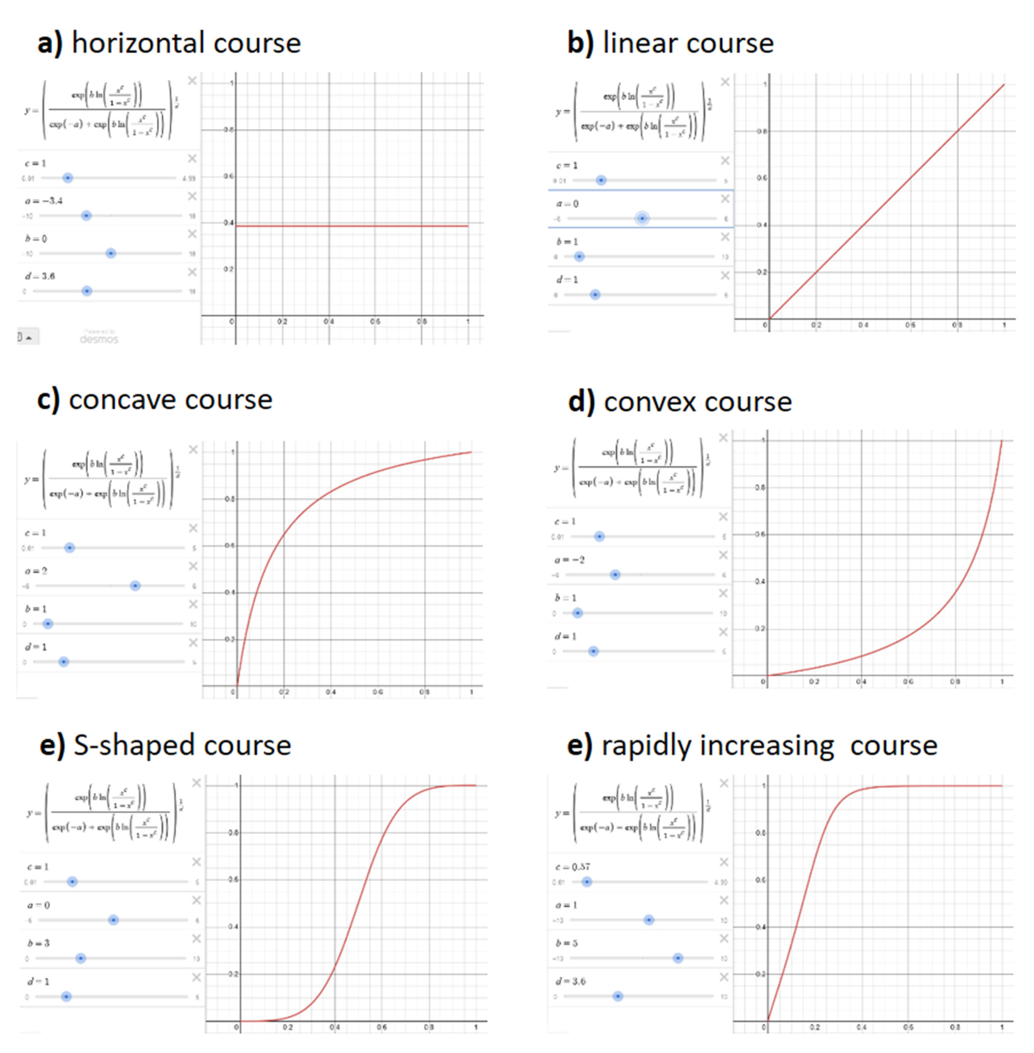

Table 1.
Parameters: Types and restrictions.
| parameter | necessary | useful range | type |
| a | unbeschränkt | -2≤a≤+2 | shift parameter |
| b | b≥0 † | 0≤b≤6 | slope parameter |
| c | c>0 | 0<c≤5 | scaling parameter |
| d | d>0 | 0<d≤5 | scaling parameter |
| u,o | u<o | u≤0.25; o≥0.75 | boundary parameters |
†so that increases monotonically with.
Disclaimer/Publisher’s Note: The statements, opinions and data contained in all publications are solely those of the individual author(s) and contributor(s) and not of MDPI and/or the editor(s). MDPI and/or the editor(s) disclaim responsibility for any injury to people or property resulting from any ideas, methods, instructions or products referred to in the content. |
© 2025 by the authors. Licensee MDPI, Basel, Switzerland. This article is an open access article distributed under the terms and conditions of the Creative Commons Attribution (CC BY) license (http://creativecommons.org/licenses/by/4.0/).
Copyright: This open access article is published under a Creative Commons CC BY 4.0 license, which permit the free download, distribution, and reuse, provided that the author and preprint are cited in any reuse.


