Avoiding Malpractice in Econometrics: “David Hendry’s Automated Methodology Nesting Theory-Driven and Data-Driven Approaches”

1. Introduction

This paper presents a concise version of Professor Hendry’s methodology, based on his books -mainly, Empirical Model Discovery and Theory Evaluation, Hendry and Doornik, 2014 (denoted as HD2014 in the rest of this paper), and Dynamic Econometrics, Hendry (1995) - and on a personal selection of his papers and of those written with associates. All these works have been very useful for me, and I have taken from them the arguments and proposals explained in this paper. I am very grateful to Katerina Juselius and Bent Nielsen for valuable comments on the paper. I am solely responsible for the selection and for the omission of relevant material and for any errors of interpretation that this paper may contain. Unless otherwise stated, the quotes in the paper come from Professor Hendry’s papers and books.

Writing about David Hendry’s methodology is a complex task, because it has many important aspects, which have been formulated, substantiated, discussed, repeatedly extended and updated and applied in a large amount of papers since 1970 and in the books mentioned above and some others. Consequently, it is difficult to have a global version of the methodology with a proper understanding of the details and statistical foundations of its main features and with some knowledge of its main applications. Given the large number of references contributing to this methodology, it has been impossible for me to contemplate them all. In spite of these deficiencies, I hope that this paper could be of interest to many readers. In fact, the paper has been written with the aim that it could be a helpful guide for those readers who are not familiar with the Hendry’s methodology and would like to have a global reliable knowledge of it. The paper also aims to be a useful summary for readers familiar with the methodology.

The “David Hendry’s methodology,” has been developed from the econometric background of the LSE, especially the work by Denis Sargan, see Sargan (1957) and Sargan (1964). In the latter reference, Professor Sargan, in the words of Hendry (2003), laid out the conceptual foundations of what has become known as the “LSE approach”. Hendry (2003) lists and analyses 10 essential elements of the methodology formalized in Sargan (1964). Many of the Sargan papers are reprinted in Sargan (1988). Thus, initially the methodology was denoted “LSE methodology” -see for instance, Mizon 1995, Hendry 2003 -, but its widest, structured, and systematic expansion with path-breaking innovations, exhaustively detailed formulations and with countless simulations has been produced along more than five decades by professor Hendry and associates. Besides, since working on his Ph. D. thesis in late sixties, professor Hendry –initially encourage by his supervisor professor Sargan- has always been worried in implementing his procedures and methodology in a software, which allows applications in an easy way. His initial GIVE program evolved to PcGive, in a personal computer framework, and later to machine-learning platforms as PcGets and finally to Autometrics. Professor Hendry’s self-imposed requirement to embed the methodology in a operative software has very much favour the formulation of the methodology in a detailed and systematic way. Thus, the methodology is rightly be named after him, see for instance, Gilbert (1986), Ericson et al. (1991).

In presenting Hendry’s methodology I, first, pay attention to its theoretical bases and then I formulate a set of features, eleven, that, in my opinion, constitute its main structure, see Table 1. Many of them are differentiating factors compared to other alternatives.

The theoretical bases of the methodology are studied in HD2014. The first element of all is the theory of dynamic econometrics -but the methodology is also valid for cross-section data- that provides the wider context for the methodology. A deep and extensive formulation of it is in Hendry (1995). Initial references are Sargan (1959 and 1961), that introduced the systems of dynamic models with autocorrelated errors, and Sargan (1964), which between other things, introduced the equilibrium correction mechanism. In the latter seminal paper, Sargan widens the framework of dynamic econometrics by including variables in levels and in differences in an econometric model for variables which exhibit trends. Sargan (1964) -see Hendry (2003) for a deep and excellent analysis of the Sargan’s contributions to Econometric Methodology in this paper- studied the wage-price inflation in UK, taking as a starting point the equations in Klein and Ball (1961). An equation for wage inflation using only variables on differences was unsatisfactory because it was not homogeneous in prices. Thus, “money wages could rise by a smaller percentage than prices, and real wages fall” (Sargan 1964, p.37). The hypothesis that the unions were sensible to real wages could be tested by introducing this variable ( a linear combination of variables in levels) in the model. In fact, it was significant. From this equation, -equation (17) in Sargan (1964)- an equilibrium solution for real wages is derived, and deviations from this equilibrium solution affect wage inflation. In this way, as stated in Hendry (2003), Sargan (1964) introduced equilibrium-correction mechanisms in econometrics.

The dynamic models with autoregressive errors determine a dynamic relationship between economic variables that is different from the dynamic structure of the residuals. Thus, in testing for autoregressive errors, Sargan emphasises that those models are special cases of a more general dynamic specification, say G, with white noise errors. The latter must be used to test, from general to specific, see Sargan (1975 and 1980), if there are common dynamic factors (COMFAC) in the structural part of the model. In this case, those factors constitute the autoregressive error structure. Models with a form G or with autoregressive errors reflect different dynamic relationships between the economic variables, which could have implications in policy. Thus, the importance of testing one formulation against the other.

A second theoretical basis of the methodology is the general-to-specific (Gets) modelling approach, that in words of Hendry (2024) really begins with Sargan (1957). A collection of readings in this topic is in Campos et al. (2005a and 2005b). The first reference, as the editors’ introduction of the readings in the second one, provides a deep study of the main aspects of Gets and a summary of the 57 articles included in Campos et al. (2005b). The Gets approach has being evolving during decades incorporating important methodological developments, as are analysed in HD2014 and Hendry (2024), see also references therein. In fact, the progressive steps in Hendry`s methodology, run in parallel with the developments of Gets, and the former can be seen as the methodological proposal derived from the long expanding history of Gets. Theoretical extensions of Gets include encompassing (see Hendry and Richard 1982, Mizon 1984, Mizon and Richard 1986 and Hendry et al. 2008); theory of reduction, model selection and misspecification tests (Hendry 1987, Sargan 1964); multi-path search (see the initial study by Hoover and Perez 1999 and also Hendry and Krolzig 1999, 2003 and 2005); multi-path search by blocks (Hendry and Krolzig 2005) with contraction and expansion phases (see Hendry and Doornik 2015, and Castle et al 2023). Also, integration and cointegration ( Granger 1981, Engle and Granger 1987); equilibrium correction mechanism (Sargan 1964, Davidson et al. 1978, Hendry 2004); exogeneity (see the seminal article Engle, Hendry and Richard 1983); robustifying models and indicator saturation estimations (see Hendry (2008), Castle et al. 2020 and 2023) and automatic model selection (see Doornik 2009 and Doornik and Hendry 2013). The above mentioned theoretical bases of the Hendry’s methodology are rooted on the statistical foundations of econometrics provided by Haavelmo (1994), that we comment with more detail in section 2.

Going back to the Hendry’s methodology, the features listed in Table 1 capture, what I considered, the four main planks of the methodology. [A] Econometric modelling is a discovery process, features 1 and 2.[B] The local data generation process (LDGP) and its nesting in a general unrestricted model (GUM), features 3 to 6. [C] A general-to-specific (Gets) reduction process from the GUM to a final congruent model, features 7 and 8.[D] Especial problems in the reduction process and their possible solutions, features 9 to 11. The first feature listed in Table 1 refers to the formulation of the aim of the methodology. This comes from the recognition that macro-econometric models must incorporate economic theories in their formulations. However, “macroeconomic theories are incomplete, incorrect and changeable” and cannot enter as restrictions in the econometric models, as it occurs with the simultaneous equation models, structural models and DSGE models. With them, a bad econometric praxis has been generated.

To avoid malpractices in econometrics, as the ones just mentioned, a given econometric empirical investigation should be directed to find a congruent model -a model based on theory and in accordance with empirical evidence (feature 1). ” This model is not given from the beginning and requires a statistical modelling process to discover it” (feature 2). The question is that “complete and correct a priori specifications almost never exist for models of observational data, so model discovery is unavoidable”.The book, Empirical Model Discovery and Theory Evaluation, HD2014), is devoted to it. This book, explains at length that the properties of an economic system must be discovered and this discovery must be the aim of economic modelling. For this purpose, economic theory must be used - without imposing it – jointly with empirical evidence. In this way, the researcher could obtain congruent models that could be used in economic policy. In many posterior papers to HD2014, Prof. Hendry has extended the scope and developed much more details of the methodology and of its statistical foundations, providing statistical profoundness, doing unlimited simulations, and making very relevant applications.

The procedure for model discovery would start from some theoretical perception -f(x_t)- that indicates a series of r variables to consider, (x_t). This initial set of variables is extended (expansion process, feature 3) with k more variables ,v_t, which include economic variables from other possible economic theories and all types of variables, situational, institutional, sociological, demographic, etc., that may be necessary to represent the economic system in question. The selected variables include “how they have been measured” (referring to the need for deterministic terms, constants, seasonal factors, trends, level changes). With the v_t variables the condition of ceteris paribus can be met. The set {w_t=(x_t,v_t)} collects all the variables that the researcher has considered that are needed for her problem.

The model building process concentrates on the Local Data Generating Process (LDGP), which is “the process by which the selected variables for the empirical study are generated including how they have been measured”. Thus, the LDGP is the joint density function of all the variables selected {w_t =(x_t,v_t)} by the researcher for the modelling process, and this function, Dw(.), is conditional on deterministic elements in the observed values and their parameters can change along time.

From a rigorous expansion procedure from f(x_t), we have arrived to Dw(.), the LDGP. But following Haavelmo (1944), it is important to derive the statistical foundation of the LDGP. This requires to obtain it from the data-generating process (DGP) of the economy on which the analyst is working (feature 4). This has been deeply studied by David Hendry (see Hendry (1995) and HD2014, chapter 6, and references therein) and other authors as Juselius (2014). In the just mentioned references by David Hendry the type of reduction operations to derived the LDGP from the DGP are formulated and analyzed with detail. HD2014, chapter 6, provides a very good summary of them.

The properties of Dw(.) are unknown and the LDGP is the aim of the empirical modelling. The way to discover the LDGP requires to nest it in a much wider context with variables capable of capturing the real properties of the system (feature 5). This involves the formulation of a Global Unrestricted Model (GUM), which contains the set of variables {w_t =(x_t,v_t)} plus some others that we analyse in section 3 of this paper (feature 6).

Then a reduction process (feature 7) following the general to specific (Gets) approach must be applied to arrive to a congruent final model (statistical adequacy) which is not dominated by any other model built over the same information set (critical resolution).

The reduction process from the GUM to a congruent final model is too complex to be resolved by a human mind and an automated program, Autometrics, (Doornail (2009), Doornik and Hendry (2013) and Hendry and Doornik (2018), has been developed for that purpose (feature 8). We will analyse Autometrics in section 8. In this framework, one very often end up having more variables than observations (feature 9). This problem is studied in HD2014, chapter 19, and in different subsequent publications by professor Hendry and associates. In those publications sophisticated procedures have been proposed that have been included in extended versions of Autometrics.

Hendry and Johansen (2015) face the problem of selection of economic theories, feature 10, in a brilliant paper. The authors consider that the selection of economic variables should be done in a way that when departing from an economic model f(x_t) that is correct, the search for additional economic variables ends up with the same estimates of the theory-parameters than a direct estimation of f(x_t). This is done by retaining the initial x_t and selecting only over the other candidates, applying, previously, an orthogonalization of them with respect x_t. Hendry and Johansen (2015) study the properties of the procedure and its possible costs and benefits.

Castle et al.(2023), in the frame of regression models, structure the above model building procedure in a context of robustness of the discovered model. Thus, they propose a general notion of robustness (feature 11) that “requires robustifying models against as many contaminating influences as possible”, (see the C1 to C8 listing in page 32 of the paper). This implies that the model selection procedure should deliver acceptable results when dealing jointly with questions such outliers -impulses or steps- and other contaminating influences, omitted variables, misspecified dynamics and non-stationary, non-linearities, having also check for the validity of the exogeneity assumptions. This is an essential aspect of Hendry’s methodology, the joint estimation of all the possible factors affecting the dependent variable. We deal below on how the jointly treatment of all explanatory variables can be addressed when there are more variables than observations. The robustifying context set by Castle et al (2023) is helpful for a clear understanding of the model building procedure.

The remaining of the paper is as follows. Section 2 comments on the reality that analysts face in empirical econometrics, and the need of a methodology. Hendry’s methodology acknowledges that a modelling discovery process is required and must start selecting a large group of variables, which are necessary to represent the economic system under study, LDGP. The formulation of the LDGP, as it has been mentioned above, can be done by an expansion process from an initial economic theory, f(xt), but also from a reduction process from the DGP, which in turn is relevant to appreciate the solid statistical foundation of the methodology. All these (features 1 t 4) are discussed in section 2. The methodology focuses on the discovery of the LDGP and the process for it, starts from the formulation of a global unrestricted model (GUM) and section 3 is devoted to it, features 5 and 6. The reduction process to arrive to a final model is studied in section 4, feature 7. Some special questions in this process are discussed in the following sections.The estimation with more variables than observations, in section 5, feature 9. Testing economic theories, feature 10, in section 6. Correction for outliers, shifts and other contaminated influences by saturated regressions, allowing at the same time for the presence of non-linear structures in the model, in section 7, feature 11. Automatic model discovery, Autometrics, in section 8, feature 8. Section 9 comments on the different uses of an econometric model and sections 10, 11 and 12 refer to discussion, conclusions and future directions.

2. The Reality Faced in Empirical Econometrics. Statistical Foundation of the Methodology Proposed by David Hendry

The reality faced in empirical econometrics is well described by David Hendry (2018) as follows. “Macroeconomic time-series data are aggregated, inaccurate, non-stationary, collinear and rarely match theoretical concepts. Macroeconomic theories are incomplete, incorrect and changeable: location shifts invalidate the law of iterated expectations so “rational expectations” are systematically biased. Empirical macro-econometric models are miss-specified in numerous ways, so economic policy often has unexpected effects, and macroeconomic forecasts go awry”.This implies: (1) that econometric models that impose economic theories, which are not tested, as Simultaneous Equation Models and structural models; or (2) that assume that the conditional distributions do not change, as the DSGE, Dynamic Stochastic General Equilibrium Model; or (3) that don’t consider all the possible variables required for the problem under study, could be not suitable for modelling economic systems and have generated econometric malpractice. For an illustration of this malpractice in DSGE models see, for example, Hendry and Muellbauer 2018, about the macro-econometric model used by the BoE. For a revision of the DSGE see Poudyal and Spanos (2022).

All this became very clear with the Great Recession that began in 2008 and more recently with CovID-19. With the Great Recession, there was already a crisis in economic ideas and critical relevant books and monograph issues in journals appeared. See, for example, the book, “Economic ideas that you should forget”, by Frey and Iselin (editors) (2017). Positive proposals followed, as those collected in the monographic issues of the Oxford Review of Economic Policy (OREP, 2018 / 1,2 ), dedicated to "Reconstructing macroeconomic theory", edited by Vines and Wills, and another book by Frey, BS and C.A. Schaitegger (Eds) (2019) 21st Century Economics. Economic Ideas You Should Read and Remember. More recently the Oxford Review of Economic Policy (OREP,2020), vol.3, edited again by Vines and Wills, was devoted to Rebuilding Macroeconomic Theory II. Also more critical references has appeared as, Akerlof, 2020, "Sins of Omission and the Practice of Economics". Shiller, R.J. 2019, Narrative Economics. King and Hay 2020 Radical Uncertainty: Decision-Making Beyond the numbers.

In a adequate econometric methodology, the models must have a solid statistical foundation. This was formulated by Haavelmo (1944). Recent references studying Haavelmo’s work are, between others, Hendry, D.F. and J. A. Doornick, 2014; Juselius, K., 2014; Hendry, D. F. and S. Johansen, 2015 and Juselius and Hoover, 2015. In Haavelmo (1944) the observed economic data (sample) are conceived as a realization of the stochastic theoretical scheme (population): the data generating process - say the LDGP above. Consequently, econometric models can only be justified insofar as they are derived from said process, finding their statistical basis in it.The LDGP has been identified with the Haavelmo distribution introduced in Haavelmo (1944).

David Hendry provides a general econometric context from which one derives the LDGP. This is explained, for instance, in Hendry (1987, 1995, 2009), Hd2014, chapter 6, and Hendry (2018). This general context refers to all the variables of an economic system and is defined as the joint density function of all those variables, and is denoted as the Data Generation Process (DGP) or, in words of Granger (1990), as the joint distribution of all the variables that determine and represent all the decisions of all economic agents. Obviously the DGP is excessively multidimensional for empirical modelling and a reduction process is required to go from the DGP to the LDGP, feature 4. This process includes (a) aggregation and (b) transformation of data as taking logs, rates of growth, etc. (c) Then a marginalization of the DGP with respect the variables which do not enter in the study of the problem under question, is applied. HD2014, chapter 6, study all the operations in this reduction process. With the remaining variables the LDGP is set up, including an appropriate contemporaneous conditioning. (d) Then, by applying a sequential factorization, the LDGP can always be written “with a martingale difference innovation that is unpredictable from the past of the process”.

It must be noted, as discussed in Hendry (2018), that “the LDGP provides an appropriate “design of experiments” whereby the passively observed data are described to within the smallest possible innovation errors given the choice of {w_t}”. The LDGP innovations are designed by the reduction process from the DGP to the LDGP and “once {w_t} is chosen, one cannot do better than know D_w(.), which encompasses all models thereof of the same data”.

The joint density function of Dw(.), the LDGP, must be correct at every sample point, which implies to work with a set of variables with appropriate lags, functional forms and stationary transformations. Besides, all the required deterministic terms must also be included in the density function. With all these additional formulations, the normal restriction could be met. Thus, it is quite clear that the LDGP must be discovered. For that aim, LDGP must be nested in a “suitable” General Unrestricted model (GUM), feature 5.

In empirical econometrics two approaches, theory-driven and data-driven, are usually employed. The Hendry’s proposal consists in nesting theory-driven and data-driven approaches, in such a way that theory-models’ parameter estimates are unaffected by selection despite searching over rival candidate variables, longer lags, functional forms, and breaks. As the author says, in this econometric modelling procedure “theory is retained, but not imposed, so can be simultaneously evaluated against a wide range of alternatives, and a better model discovered when the theory is incomplete.” The theory is included in the LDGP, but this joint density function also includes other economic variables.

On the contrary, the theory-driven approach maintains that the theoretical model chosen by the analyst is the economic mechanism that underlies reality and a “ceteris paribus” condition is assumed, that is, the other conditions not included in the model remain constant. That assumption is the big mistake. Thus the goal should be to capture the entire mechanism behind the data. If not, the statistical inference may be invalid.

Hendry (2018) gives an excellent illustration of the problem with the modelling of the Phillips curve, relating wage inflation with unemployment, from an annual sample since 1850. Both variables show a number of location shifts in this period, that in many cases are in common but not necessarily overlap. Consequently, the Phillips curves show shifts in different periods. As Hendry argues, these findings do not “entail that there is not constant relationship between wage inflation and unemployment, merely that a bivariate Phillips curve is not such a relation”. Additional variables must be included as it is done in Castle and Hendry (2014). Thus the shifts can be modelled and the underlying economic behaviour can be understood.

Regarding to the data-driven approach, clearly empirical evidence is necessary for the selection of econometric models, but as Hendry (2018) indicates, it is not sufficient. The model building process concentrate on the Local Data Generating Process (LDGP), and the selection of variables which have being include in it “must be made taken ideas from theory”. Consequently, with empirical evidence alone we cannot obtain an appropriate model for our study.

In the data-driven approach the argument of choosing as a final model ”the one resulting from the maximization of the goodness of fit or the likelihood function, is correct for estimating a given specification, but incorrect for selecting a specification”. As David Hendry argues, the best-fitting model: 1) may show systematic deviations in the data, such as autocorrelation and heteroscedasticity and several others. Therefore, additional criteria are necessary to ensure that the models fit the characteristics of the data. Furthermore, 2) they do not guarantee understanding compared to alternative models. The final model must be a model that is not dominated by any other that can be built with the same information set. The final model must encompass the GUM.

Hendry and Doornik (2014) propose a mixed procedure based on a loose theory and in accordance with empirical evidence. From the above considerations it follows that the information set with which we have to work to build the econometric model must contain variables based on economic theory, but also variables that capture everything that is inappropriate in the ceteris paribus assumption.

3. Formulation of a General Unrestricted Model (Gum)

Consistent with what has been discussed above, the construction of an econometric model must start from a GUM, see, for instance, Hendry and Doornik (2014), chapter 7, Hendry (2018) and Castle et al. (2023). “Three extensions to w_t can be automatically implemented to create the GUM, namely functional-form transformations for non-linearities, indicator variables to capture outliers, shifts and other contaminated influences, and dynamics.”

Thus, the GUM must include (see Table 2, based on equation (15) in Hendry 2018) :

-

the n economic variables, x_t, defined in a specific theoretical model;

-

additional economic variables that could also be of interest, and all kinds of variables, conjunctural, institutional, sociological, demographic, etc., that may be necessary to represent the economic system in question. With them, the condition of ceteris paribus can be fulfilled. This is a vector v_t, of k variables. (Thus the vector of all variables is w_t=(x_t:v_t) and the number of variables is r=n+k.)

-

A specific proposal to capture non-linearities. Hendry (2018) proposes 3 non-linear functions –quadratic, cubic and exponential- of the principal components of w_t.

-

All the lags till order s for w_t=(x_t:v_t) and for the non-lineal functions and

-

Variables for the indicator saturation analysis -we discuss saturated regressions in section 7-, generalized in Castle et al.(2023) to five type of indicators: IIS, impulse indicators, SSI, step indicators,TIS, trend indicators, DIS, designed indicators for specific shapes and MIS, indicator for changes in the parameters of other variables (proposed by Ericson 2012).

In order to formulate a GUM that really could be a solid foundation for the empirical analysis in question, Hendry and Doornik (2014), section 7.3, propose the following. “The GUM should be based on the best subject-matter theory, institutional knowledge, historical contingencies, data availability and measurement information”. The GUM must be a valid representation of the data under study and for that purpose a set of mis-specification tests are applied to the GUM. If some mis-specification test fail, then a reformulation of the GUM should be done and should be submitted to the set of miss-specifications tests. The procedure continues until a GUM is not rejected.

4. The Reduction Process

Specific references for this section are Hendry and Doornik (2014), chapters 7, 11 and 13; Doornik and Hendry (2013 and 2015) and Hendry (2018) section 7.2.

The reduction process from the GUM to a final congruent model is carried out by the procedure from general-to-especific (Gets) and it is based on two main bases: statistical adequacy and critical resolution. The procedure explores the elimination of each variable, generating a structured process of multiple reduction paths, explained bellow. Two requirements are applied to select a model corresponding to each reduction. One refers to the fact that the reduced model must encompass the GUM, meaning that it explains the results of the GUM. This can be checked using an F-test and in this methodology is denoted as back-testing. Since the GUM includes the true LDGP, all valid simplifications of the GUM are well specified. Under the second requirement, the reduced model must undergo a battery of diagnostic tests that ensures that the it is congruent with the data; “goodness of fit is not a sufficient criterion in a search process”. Congruence with the data for a specific model requires that tests on heteroskedasticity, autocorrelation, normality, autoregressive conditional heteroskedasticity, exogeneity, non-linearity, parametric stability and encompassing with respect to alternative models, are applied and satisfactorily passed.

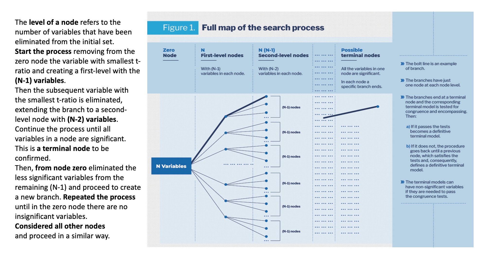
In the structured process of multiple paths used in the reduction process, the paths are also called branches and the whole procedure can be referred as a tree search. It starts from a GUM with N variables. For the reduction process, we denote this set of variables as zero node and from it, nodes of different levels will be derived, as shown in Figure 1. The level of a node refers to the number of variables that have been eliminated from the initial set of N variables. The first step in the reduction process consists in removing from the zero node the variable that has the smallest absolute t-ratio, creating a first-level node with the (N-1) remaining variables. From it, the subsequent variable with smallest t-ratio is eliminated, extending the branch to a second-level node with (N-2) variables. By successively removing the variable with smallest t ratio from the set of variables in the previous node, the process continue until all variables in a node are significant. This is then a terminal-level node, which should be confirmed. This path from node to node with the elimination in each case of the less significant variable, constitutes the first branch in the searching process. The bold line in the Figure 1. Then the specification of the model at the end of the branch is tested for congruence with the data and for encompassing with respect the GUM. If the model pass the tests, is confirmed as terminal. If not the procedure goes back until a previous node which satisfies the tests. The corresponding node and model are then classified as terminal.

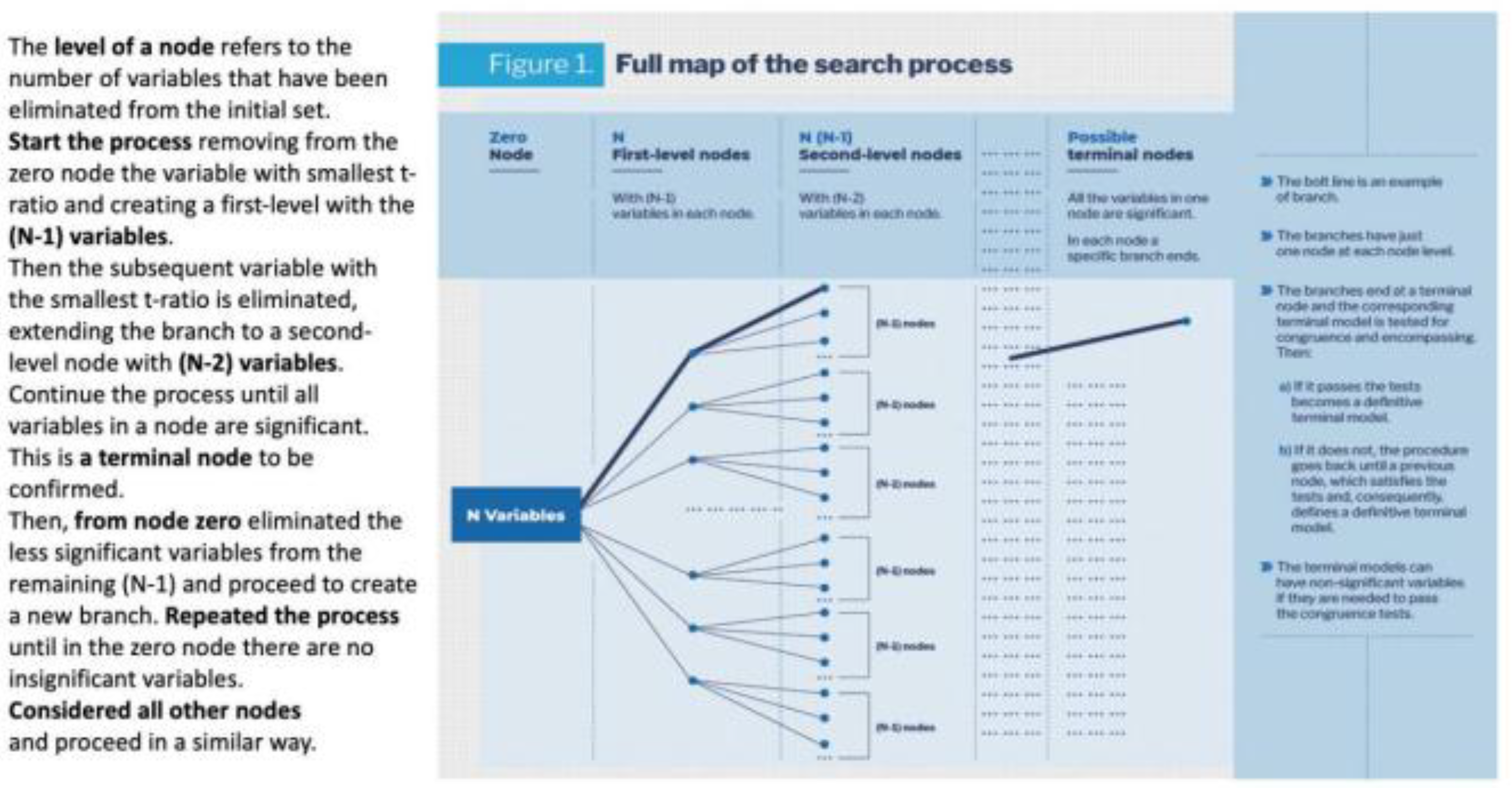
Next, returning to the zero node, the less significant variable of the (N-1) variables, which still have to be considered, would be eliminated and proceeding as before a new branch is formulated ending with a terminal-level node with a terminal model, which will be defined and tested. This is repeated until in the zero node there are no insignificant variables to start a new branch. It must be noted that the branches have just one node at each node level before the terminal node. Also the branches do not necessary have the same number of nodes, because a branch ends when in a node there are no insignificant variables.

To complete the formulation of the tree of reduction paths, we must considered all other nodes of node levels different from zero and define other sub-branches –we still denote them also as branches-, which will follow until in each branch a node has not insignificant variables to continue the branch. All these possible branches should be specified and from them terminal models will be defined and tested. Nevertheless, a learning process emerges in the search. In fact, in the tree search there are nodes with the same variables than in nodes of previous branches that have already being tested. The process learns from the previous tests and simplifies the search. It must also be noted that in a terminal model non-significant variables could be included if by eliminating them the back-testing or diagnostic tests fail.

The above discussion shows that this procedure is a structured process, which explores all the possible reduction paths from an initial set of N variables. The structure has been built making use of different level nodes, see Figure 1. The node zero has N variables and eliminating a different one in each case, we create N first-level nodes with (N-1) variables in each one. In the next step we eliminate a different variable from each one of the N first-level nodes. Thus we generate Nx(N-1) second-level nodes with (N-2) variables in each. Proceeding in a similar form, we create third-level, fourth-level nodes, etc. Then by defining all the possible paths from the first-level nodes till the terminal-level nodes we have the whole multiple-path structure of the reduction process. This formulation of the branches ending in a terminal node, implies that the possible continuations of the brunches from terminal nodes are invalid and, consequently, they are ignored, “pruned” in the terminology of HD2014.

In this reduction process a huge total number of N^2 models could appear. But, Autometrics simplifies the process by strategies to skip nodes and by learning as searching, as mentioned above. Another strategy, besides pruning, consists on working along a given branch with a bunch of variables and test if the whole bunch or a part of it can be jointly deleted.

With the union of all the terminal models, HD2014, chapter 13, propose to define a new GUM, GUM₁, and start a new tree search, which will lead to a new GUM₂ and so on. The process ends when GUM_i is the same as GUM_i-1. The multi-path search can conclude with several terminal models that encompass the GUM and are congruent. In this case, the final selection can be made by information criteria or by applying broad modelling, as proposed by Granger and Jeon (2004). In sum, given the initial GUM, this selection process looks for the “simplest acceptable representation thereof” and it is carried out by “stringently evaluating it for congruence and encompassing”. The procedure leads to a congruent final model (statistical adequacy), which is not dominated by any other model built over the same information set (critical resolution).

Since the earlier years of this methodology, Professor Hendry has analyzed that in the searching processes we can distinguish two types of costs.The inference cost, which is due to the fact that in testing hypotheses, the probability of rejecting the null when it is correct (α) is not zero. It is therefore an inevitable cost. Thus, even starting with the (true) LDGP and not being sure that it is correct, it needs to be verified and α% of the time we would incur the cost of rejecting it. The search cost is an additional cost for not testing on the LDGP, but rather on a broader set, GUM, that includes it. In this reduction process we are not looking for a congruent model, because the reduction departs from the GUM, which is congruent with the data. We look for invalid reductions that can be left apart.

The statement that in the reduction process "multiple testing does not take place" is associated with the fact that even though the search for all possible paths involves a very large number of tests (N! - factorial of N-), that does not mean "repeating" N! tests. In fact, the approach in the reduction process is different. It consists in searching the true specification within a wide set of specifications, which include the true one, applying a battery of stringent enough specification tests. White (1990) shows that, in this context, asymptotically the test battery will select, with a probability approaching unity, the correct specification. This means that having enough data, searching in a proper set and being stringent, the true specification will emerge. Besides in Hendry’s methodology the reduction process requires encompassing the GUM and satisfying congruency with data. Therefore it is important not to confuse multi-path search from a GUM with N variables (which includes the true model), with the selection of a model with the best fit from approximately 2^N possible models.

Hendry (2018), section 7, proposed three ways to judge the success of structured selection algorithms as the one incorporated in his methodology and applied it in the automated program Autometrics. They are as follows.1) The algorithm should recover the LDGP from the GUM. 2) “The operating characteristics of any algorithm should match its stated properties”. For instance, between other things, this means that the null rejection frequency (gauge) and the retention frequency for relevant variables (potency) should, correspondingly, “be close to the claimed nominal significance level (denoted α) used in selection” and “preferably be close to the corresponding power for the equivalent tests on the LDGP”. As noted in Hendry (2018) “gauge and potency differs from size and power because selection algorithms can retained variables whose estimated coefficients are insignificant on the selection statistic. The definitions of Gauge and Potency were formally introduced in Hendry and Santos (2010). 3) The algorithm used in the reduction process “should always find at least a well-specified, undominated model of the LDGP”.

The simulation results reported in several papers by Hendry and associates indicate that these three measures can be reached with reasonable success and show that the searching costs are surprisingly small relative to inference costs. Castle et al. (2011) show that the retention rate of irrelevant variables ( gauge) when selecting from a candidate set of variables is close to the pre-set nominal significance level α for α = min(1/N, 1/T, 1%), so that on average just αN ≤ 1 spuriously significant variables will be retained. Besides, relevant variables will be retained with roughly the same frequency ( potency) as the power of the corresponding t tests at α in the LDGP. That is to say, that searching for the true model in a broad set that includes it, does not have a high additional cost. The main reason is that the search is done in a set that contains the null and all possible reduction trajectories are considered.

Hendry and Doornik (2014) also compare by simulation methods the performance of Autometrtics with the performances of other approaches as step-wise regression (a general-to-specific approach), information criteria (AIC, Akaike 1973, BIC, Schwarz 1978), Lasso (Tibshirani 1996), RETINA ( Perez-Amaral et al. 2003 and 2005), Hoover-Perez algorithm ( Hoover and Perez 1999) and PcGets ( Campos et al. 2005). They conclude that in many settings the results with Autometrics are better than those from the alternatives and that they don’t necessary deteriorate having more variables than observations. Some alternatives can outperform Autometrics in some occasions, but they appear “not reliable and can also deliver very poor results”.

Nevertheless, “the estimates from the selected model do not have the same properties as if the LDGP equation had just been estimated”. Thus the estimated parameters will be biased. Correction for the biases due to selecting only significant outcomes is provided in Hendry and Krolzig (2005), and is described in HD 2014, chapter 10. In any case, the bias correction carries a “little loss of efficiency from testing irrelevant variables”. A more problematic question refers to the fact that “when relevant variables are omitted and are correlated by retained variables, the latter coefficient estimates may or may not be corrected” by the procedure in HD2014. Then a low α value will help in retaining relevant variables of low significance, but at the risk of retaining irrelevant variables. This trade off must be carefully considered in an empirical application, and HD2014 provide several considerations to choose the value of α, which could depend on the purpose of the final model and “different choices of α can be justified”.

The above description shows that the aim of the reduction process from the GUM is that the analyst could select “the model that is the most parsimonious, congruent, encompassing model at the chosen significance level to ensure an undominated selection, controlling the probability of accidentally significant findings at the desired level, computing bias-corrected parameter estimates for appropriate quantification. Stringently evaluate the results, especially super exogeneity, to ensure that the selected model is robust to policy changes. ”.(Hendry 2018, page 133). From the final congruent model, the confirmation of the initial theory, a modification of it or a new theory will be derived.

In many cases, at the starting point there is a number of variables greater than the number of observations, and Professor Hendry has been developing a block modelling methodology with expansion and contraction phases to solve the problem, which has also been implemented in Autometrics. In the next section we comment on it.

5. Estimation with More Variables than Observations. Cemps, Contracting and Expanding Multiple-Paths Searches

This section is based on HD2014, chapter 19, Doornik and Hendry (2015) and Castle et al. (2023, section 3).

In the methodology that we are analyzing, there are several questions that professor Hendry has had to address, studying them analytically and by performing a great number of simulations. All this is presented in HD2014 and in subsequent papers. In this and following sections, I would like to comment on some of those questions.

The case of more variables (n+k) than observations (T) is faced using (A) the tree search or multiple-paths searches, described in section 4, but (B) implementing it using segmentation by blocks. Besides, (C) the block strategy is complemented with expansive and contractive phases, HD 2014, ch 19. Hendry (2024) denotes the whole procedure as CEMPS, contracting and expanding multiple-paths searches.

The block search proposed in Hendry and Krolzig (2005) is as follows. (1) Split randomly the N variables into K blocks, with K≥ 2, smaller than T/2 and with α=1/N. (2) Apply Gets to each of the K(K-1)/2 block pairs to reduce the variables. In each pair Gi variables will be selected.( 3) Take the union M of the significant variables in each terminal model (Gi's) and form with M a new GUM. (4) Repeat the process until M is strictly smaller than T and the usual process can be applied. The following example is taken from Hendry and Doornik (2014). If there are three blocks A, B and C, and Gets is applied to the three possible pairs of blocks and three sets of final variables are obtained G1 (from pair A and B), G2 (from pair A and C) and G3 (from pair B and C). Then new GUM is the union of G1, G2 and G3.

As pointed out in HD2014,section 19.2, the above procedure has the inconvenient that if a relevant variable is missed in testing in all block pairs, there is not a later recovering process for them. Thus, they propose the selection by blocks mentioned above but with contracting and expanding phases, see also Doornik and Hendry 2015.In the block search just described, each iteration ends with a set of M_i significant variables, which are selected, and, say, with Rⁱ non-selected variables. If necessary, a new iteration (i+1) starts with a GUM formed with the M_i variables. Now in the selection by blocks with expansion and contraction steps, the procedure is amplified as follows. At the start of any iteration i+1, there is an expansion step, which tries to recover some of the non-selected variables Rⁱ. Thus, the Rⁱ variables are partitioned by blocks [Rⁱ₀… Rⁱ_r] and the procedure runs r reductions in Rⁱ₀ Ս M_i, …, Rⁱ_r Ս M_i,.maintaining M_i..The resulting significant variables in [Rⁱ₀… Rⁱ_r] are selected in R1. If the dimension of R1 is not sufficiently small, a partition of R1 in blocks is done and the process is repeated with them. Continue repeating the process until the selected set R at repetition (i+1) is the same than the selected set of the previous iteration. After this expansion step we have as potential variables M_i Ս R and a reduction step is applied to it. It consists on running the iteration (i+1) in the block search with M_i Ս R from which an M_i+1 will emerge. The iterations will continue until the dimension of the current M_i is suitable for the standard procedure with more observations than variables, and no new significant variables in the set of omitted variables emerges in further searches.It is important to note that in the expanding steps all non-previously-selected blocks of variables are considered, but in the contraction steps the new-selected variables are test in a model with the currently candidate variables.

Castle et al. (2023) propose a more detailed CEMPS procedure, controlling the sizes of the blocks and allowing for a subset of variables, which are retained in the selection process but estimating their coefficients.

The empirical modelling discovery strategy that we are analyzing, is based on a starting general unrestricted model GUM, which is tested for mis-specifications, and on a subsequent reduction process. As Doornik and Hendry (2015) point out, when we have more variables than observations, the GUM can´t be tested for mis-specifications. Then as these authors say, the program “selects as if the estimable sub-models were well specified, and seeks to move to a final choice that is congruent”.

When the collinearity between the variables is high, the process of selecting variables can be difficult. In those cases HD2014 suggest to substitute the variables by their principal components -which by construction are orthogonal- and make the model selection on them. The cost is that the estimated coefficients have not a direct interpretation. Another possibility is orthogonalizing the regressors. We comment this approach in the next section.

6. Testing Economic Theories

In testing economic theories, one would like to maintain the theory when it is true and find alternatives when it is false. This is the question studied in Hendry and Johansen (2015). They assume a theoretical model with n regressors, x_t,:

y_t= β’x_t + e_t,

(6.1)

which is nested in a broader one that includes k additional regressors, v_t,:

y_t = β’ x_t + γ’v_t + ε_t.

(6.2)

The selection procedure is carried over the set {x_t.v_t} of n+k variables, but they introduce two important points in the process. a) The seleccion does not apply to the x_t variables, which are always retained; and b) the selection goes over the η_t variables, which result from the orthogonalization of v_t with respect x_t. Thus,

v_t = x_t + η_t and

y_t = β₊^´x_t + γ’η_t + ε_t,

(6.3)

where β₊ = β + Γ`γ.

The theoretical model needs to be complete and correct, which implies that in the theoretical model: a) “there are no omitted variables that are relevant in the data generation process (DGP), b) the model does not include “variables that are irrelevant in the DGP”, and c) “and all included variables [in the model] enter with the same functional forms as in the DGP”.

When the theory is correct, γ’=0. This procedure, which maintains x_t, and searches over many candidates which have been previously orthogonalized, provides the same theory-parameters estimates than a direct fitting of the theoretical model (5.1). As shown in Hendry and Johansen (2015), for a Gaussian distribution and fixed regressors, the distribution of the theory-parameter estimates is not affected by this selection process, which turns to be costless.

Nevertheless, this selection process, in general, has some possible costs, even when some benefits are also possible. As explained in Hendry and Johansen (2015), see also HD2014, one cost refers to the case that even when all v_t regressors are irrelevant, we can expect to find αk of them significant, where α is the significant level of the tests. Thus some confusion could arise on the theoretical model. The above references argue about some rule to reject the theory-based model, for instance when more than one v_t variables are significant. Another cost refers to the biased estimator of the residual standard deviation, but it can be corrected under the null. One important possible benefit lies in the fact that the theory-based model is evaluated against many alternatives and if the model is incorrect, the benefit of a better final model will emerge. For all this, HD2014 state that the procedure generates a win-win situation.

In the more general case on which the number of variables, N= n+k, exceeds the number of observations, T, but n˂˂T, the procedure for testing economic theory can also be applied, but orthogonalizing by blocks and selecting, as above, on the v_t variables while retaining the theoretical variables, x_t, at every stage.

7. Outliers. Robust Estimation. Indicator Saturation Estimation. Treatment of Non-Linearities. Testing Super Exogeneity

The presence of outliers -usually multiple outliers- and shifts in economic time series is quite general and they prevent the normality assumption and can distort statistical inference. Consequently, in an empirical application the researcher must take account of them. The traditional approach has followed the methodology from single to general. Thus, to detect impulse outliers it was quite common to include impulse dummies one by one and selecting the model with the maximum t-statistic associated with a particular dummy. Having selected a date for an outlier, the procedure repeats until no more outliers are found. This procedure, as described in HD2014, has several drawbacks. Location shifts and impulses can be confused, the procedure can fail when there are sequences of outliers and the estimations can be biased.

An alternative approach in the tradition of the general-to-specific methodology is the Indicator saturation estimation (ISE), invented by Professor Hendry, see for instance, Hendry et al. (2008), Castle and Hendry (2020), Castle et al. (2023) and Hendry (2024). Along the years, professor Hendry and associates have developed different types of indicator saturation estimators. Castle et al. (2023) describes them, by considering the “five indicator-saturation techniques that have seen empirical application”. They have been designed to correct for outliers (IIS), location shifts (SIS), breaks in trends (TIS), specific shapes (DIS) and parameter changes (MIS). We comment on them along this section. Ericson (2012) already defined several types of ISE, see Table 1 in this reference, which are a generalization of the initial and simplest ISE, called IIS, which we analyse in section7.1. The ISE generates an indicator for every observation in the sample and, therefore, with it we always face a case of more variables than observations that we have discussed in section 5.

7.1. Impulse-Indicator Saturation, IIS. Testing Super Exogeneity

The first ISE that appeared in this literature was the impulse-indicator saturation (IIS), whose feasibility in Hendry (1999), was in the words of the author a “serendipitous discovery”. The IIS was formally proposed by Hendry et al. (2008) for independent identically distributed data and generalized in Johansen and Nielsen (2009) for stationary dynamic and unit-root autoregressions. A deeper and extended study is in HD2014, chapters 15 and 20.

For IIS we need to create T impulse indicators, d_jt = 1[j=t] for j=1,…T, one per observation. These indicators must enter in the regression by groups, that was the “serendipitous discovery”, because the inclusion of all of them, obviously, will provide a perfect fit. Initially the split-half method was used and was implemented in three steps. Firstly, half of the indicators corresponding to the first T/2 observations are included in the regression and we record those that are statistically significant. The authors suggest α= 0.55% (2.77σ). Next, we remove those indicators and include the other half, run a regression with them and record the significant ones. In a third step, we use the union of the selected indicators in the two previous regressions, run a final regression with them and re-select from this regression, possibly with α= 0.05. The ‘split-half’ analysis is “the simplest specialization of a multiple-path block search algorithm.” Thus, Hendry et al. (2008) consider other ways to split the sample, for instance r splits of T/r observations each and show that they “do not affect either the null outcome” when there are no outliers.

Doornik- and Hendry (2016) commenting on Johansen and Nielsen (2016) emphasize that the outliers correction is a type of robust estimation and argue that the model selection and robust estimation must be run jointly. Consequently the outlier correction that we are discussing in this section must be jointly done with the model selection that we have analyzed in section 4. We see now that the IIS makes it possible.Thus the GUM in section 3, as we mentioned then, must include the select variables jointly with the IIS. Even more, we will see below, that to correct for shifts, breaks and parameter changes we need other types of indicator saturation and all of them must be included, when this is the case, in the GUM. This turns to be an advantage of the ISE, the selection of indicators by saturation can (must) be done jointly with the selection of variables, dynamics and non-linear structures. Then it becomes clear that the detection of outliers, and also the detection of other “contaminating influences” modelled by ISE, is done with reference to a model and no respect to the data. Besides, as pointed out by Castle et al. (2023), these selection methods where first developed -HD2014- for time series models, but they can also be applied to cross-section models as the applications in their paper show.

Thus, the procedure described above to implement IIS must be generalized and this has been done in Autometrics, using the selection algorithm for the cases of more variables than observations, therefore using block searching , CEMPS, described in section 5. Now, each impulse indicator is treated as a variable. The feasibility of IIS, which was pointed out in Hendry (1999), has been based on selecting from the T indicators, using blocks of indicators. Initially as the split-half method or other split-T/r alternatives in Hendry et al. (2008) and, finally, it has been firmly established by the use of the CEMPS in Autometrics. The block estimation applied to IIS has had a special impact in the question of estimation when we have more variables than observations.

We should remember that the retention of regressors (including indicators for saturated regressions) is not only derived by a significance criteria, but criteria for congruence are also considered. Thus, non-significant indicators at the target value can be retained.

As it is clear from the different points that we have already discussed, the use of the IIS is important to fulfil the normality assumption and avoid distortions on inference. Besides, it has contributed to advances in the treatment of several questions as the dealing with more variables than observations and as we will see in the next section, in testing non-linearities.

Also, Hd2014, chapter 22, shows how IIS can be used for testing super exogeneity. They propose to do it in two steps. First, applying IIS to the to the policy exogenous variables, and then testing if the significant indicators found on them, are also significant when added to the conditional model of our variable of interest. If they are not, we can consider these policy variables as super exogenous.

The asymptotic properties of the IIS under the null were studied by Hendry et al (2008) and extended in Johansen and Nielsen (2009) to stationary dynamic and unit-root autoregressions. Jiao and Nielsen (2017) extended the asymptotic results allowing the ”cut-off value to vary with sample size and iteration step”. When there are no outliers and with α= 1/T,the procedure will retain on average just one indicator. We have not an asymptotic theory under the presence of outliers, and Jiao and Nielsen (2017) recognize the interest of extending their “results to situations where outliers are actually present in the data generating process”. For the case of Least Trimmed Squares (LTS), Berenguer-Rico and Nielsen (2024), departing from an LTS model proposed by Berenguer-Rico et al. (2023), in which the LTS estimator is maximum likelihood, provide the asymptotic theory of the regression estimation when there are leverage points in the data set, and show that the derived asymptomatic theory does not depend on the outliers. For model selection procedures as Autometrics, the asymptotic theory include nuisance paremeters, but the analysis in Berenguer-Rico and Nielsen (2024), as they say, “opens up new inferential procedures in the presence of outliers”.

In spite of the advanced mentioned results, the properties of the IIS estimation have been studied by Monte Carlo experiments, see for instance Castle et al. (2012), and the results indicate that Autometrics performs quite well selecting variables and indicators under all the specifications considered in the experiments. Castle et al. (2015) mentioned several references with successful applications of IIS. Other initial economic applications of IIS have been provided by, e.g., Ericsson and Reisman (2012), Hendry and Mizon (2011), and Hendry and Pretis (2013).

7.2. Step-Indicator Saturation, SIS. Selecting Non-Linear Models

Another type of contamination in the data consists on location shifts or changes in previous unconditional means. The IIS has also been used to find some location shifts, see Castle et al. (2012) and HD24, chapter 20. But the step-indicator saturation, SIS, another one of the five indicators considered in Castle et al. (2023), was introduced by Castle et al. (2015) to deal specifically with location shifts.

Now in the SIS the indicators are S_t (τ) step variables with value zero for t>τ, and value 1 for t≤τ. The saturation includes S_t (τ) variables from t=1 to t=T, noting that S_T(τ) is the intercept. Also, a truncated step between observations T1 and T2 requires two steps indicators S_T1(τ) and S_T2 (τ). Castle et al. (2015) apply the SIS using split-half approach or splits with other proportion of observations. But due to the multicollinearity between the indicators, a multi-path search is important, so the CEMPS methods should be applied, HD2014.The implementation of SIS with this block-search algorithm can be denoted as a general SIS algorithm in contrast with what could be denoted, see Nielsen and Qian (2023), as a simplified SIS algorithm, for instance, split-half SIS. The later is most convenient to study the statistical properties of SIS algorithms, and as these authors mention “simulations by Castle et al. (2015) indicate that the general SIS has the same gauge properties as split-half SIS”. The advantage of general SIS is that, according to the mentioned simulations it “can detect a wider range of shifts with more power”.

It must be noted that when the selection of indicators is done jointly with regressors, the latter ones are retained without selection.

The IIS and the SIS are closely related procedures, since an impulse indicator is the first difference of the step indicator for the same date and a step indicator is the integration (sum) of all the impulse indicators till the reference date of the step. Therefore the SIS can be used to detect impulse outliers, but the IIS has more potency for this analysis and is preferred. Similarly, the IIS can be used for location shifts -we have mentioned it above- but for potency reasons SIS is preferred. Nevertheless, this is different of what is called super saturation -see Ericson (2012) and Castle et al (2015)- which is the application of both the IIS and SIS, each one on its own nature: impulses and steps, respectively. Simulations and some applications show that, in general, super saturation works better than just only one of two approaches.

In section 3, when formulating the GUM, we discussed that non-linear structures could matter in the DGP and comment that to take account of possible non-linearities, HD2014, chapter 21, proposed to include additional variables as squares, cubics and exponentials of the principal components of the variables. The question is that non-linearities can generate extreme observations, which could be difficult to distinguish from extreme observations that are outliers. Then, if true outliers are not modelled, spurious non-linearities could appear and, the opposite, removing outliers could risk to remove true non-linearities.

In HD2014, the authors propose to apply IIS, which does not remove the outliers, but includes in the model indicators to take account of possible outliers. Therefore, the model selection, described in section 4, is done jointly with IIS and non-linear factors, as those mentioned above. Thus, both, contaminated and non-linear data hypotheses have a chance. HD2014 comment on the dangers of including in the model irrelevant non-linearities and propose a “super-conservative strategy”, page 260, designed, to retain non-linear factors only when there is “definite evidence” in their favour. This strategy has two steps. First, using a stringent critical value, non-linear factors are tested, retaining all other elements in the GUM, included selected indicators. Then, with a looser level, made a free selection of all elements in the GUM, including the selected non-linear factors in the first stage, if any.

Castle et al. (2015) give additional evidence of the importance of jointly selecting non-linear factors and, in this case, step indicators. They conclude that “SIS can act as an insurance mechanism in non-linear models.” This is so because, the SIS has little effect on inference when non-linear factors are present. On the other hand, when there are not non-linear factors but the data experiences shifts, the application of SIS works well on identifying steps and rejecting non-linearities. Castle et al.(2023) also analyses the question of discriminating between non-linearities and outliers and confirms that “jointly selecting impulse indicators and non-linear functions enables discrimination between these hypotheses.”

Nielsen and Qian (2023) mentioned the growing importance of SIS in tackling location shifts and provide references for applications of SIS in economics, climate science and public health. This paper acknowledge that there is no study of the asymptotic properties of SIS and it is devoted to provide some results using asymptotic analysis and simulations.

We have seen the importance of detecting structural breaks using model selection. Besides they can be related, between other things, to policy interventions, but to ascribe them to interventions, the question of uncertainty around the dates of the estimated breaks must be addressed. This question motivated the paper by Hendry and Pretis (2023). They formulate the detection of breaks as a model selection problem -in the way that we have seen along this paper-, and design a smart procedure to address the uncertainty around the dates. They assume normality in the errors terms that could be guaranteed in the context of Hendry’s methodology. In Hendry and Pretis (2023) the authors consider the possibility of just one true break of magnitude δ at observation T₀, but they are interested in extending the study to multiple breaks. Then they apply a step saturation analysis for a period T_0-k to T_0+l and establish conditions to rank the different break functions. From these results, they determine the probability of the retained break date coinciding with the true break and also are able to construct approximate confidence intervals around the break dates. In an application to the UK annual growth rates in emissions of nitrogen oxides for the time period of 1970-2019, during which multiple policy interventions have been implemented, they conclude that the estimated breaks can be associate with policy inventions.

7.3. Multiplicative-Indicator Saturation (MIS)

Another indicator-saturation, denoted as MIS, multiplicative-indicator saturation, has been designed to capture changes in the coefficients of the variables in the GUM. It was proposed in Ericson (2012), see also Ericson (2017). If the analyst suspects that the coefficient of a specific variable, x_it, of the GUM has changed at time r, the indicator to capture that possible change would be the product of the step indicator, Sr_t, and the variable,x_it,: Sr_tx_it. Then, both variables, x_it and Sr_tx_it, would be included in the model, and if the coefficient of Sr_tx_it appears significant in the estimation, it would confirm the break. In general, there could be more suspected breaking points at unknown dates and in several other variables, say k, then we will run a saturated regression with Sr_tx_it indicators for all the T observations and all the k variables. Thus, this saturation could detect changes in the parameter of the variables in the GUM.

An interesting application of MIS referred in Hendry (2024) consists in testing changes in the dynamics of the dependent variable. If applying SIS we find some significant location shifts, interacting those indicators with the lags of the dependent variable, we could discriminate “between direct shifts and those induced by changes in dynamics”.

7.4. Designed-Indicator Saturation (DIS)

Another indicator-saturation method, denoted DIS -designed-indicator saturation- consists in designing specific indicators with a particular form to account for certain effects that have a common reaction ‘shape’, which could be present in the variable of interest. This ISE was introduced by Pretis et al. (2016) to analyse the relationship between volcanic activity and temperatures. DIS is a complete generalization of ISE. It opens a new way to saturated regressions, which are appropriately designed for the economic problem in question.

7.5. Trend-Indicator Saturation (TIS)

Finally, we have a fifth ISE denoted trend-indicator saturation, TIS, proposed by Castle et al (2019) to deal with breaks in linear trends. It has been referred in Castle et al. (2023), Hendry (2024) and others.We mentioned above that a step-indicator -S_t (τ)- is the integration (sum) of an impulse (d_jt), similarly, the integration (sum) of the step, St (τ), is the trend-indicator T_t(τ) use in TIS. On that logic, Ericson (2012) denotes ultra saturation when the three indicators impulse, step and trend are used in a saturation regression. The question of trends in economics has been considered for long time and a main problem is that they are not constant. Consequently, trend-indicator saturation could be of interest, as shown by the applications mentioned in Castle et al. (2019).

8. Machine Learning Automatic Model Discovery. Autometrics

The aim of the Hendry’s methodology is to find a final congruent model. But this model is not known at the beginning of the investigation and it must be discovered by a modelling process. It must start from a General Unrestricted Model (GUM) and then through a “reduction process”, following the general-to-specific approach, aims to arrive to this congruent model. In this methodology the reduction process, and possibly the formulation of the GUM, are too complex and an automated machine-learning program is required. Autometrics, Doornik (2009) and Hendry and Doornik (2013), has been developed for that purpose.

David Hendry’s research is characterized by his insistence that the theoretical procedures and methodology formulations derived from his theoretical papers, should be implemented in a software which could be applied in empirical works. In his Ph. D. thesis, 1970, he developed the GIVE program, that few years later was built for pc’s, the PCGive Program. Escribano (1995) contains a review of the professional version of the program and references by other authors of the reviews of previous versions of the program. After the work in Hoover and Perez (1999) that propose multi-path search in Gets, generating important improvements, Hendry and Krolzig (1999) formulate PcGets, an automated model selection program. This program is also implemented in R, see Pretis et al. (2018), and in Eviews, see EViews (2020).

Finally Autometrics, Doornik (2009) and Hendry and Doornik (2013), departing from PcGets, is an automated machine-learning platform including tree-search and the advances on encompassing and reduction theory. Autometrics continues incorporating all the methodological innovations that we have discussed in previous sections, mainly the contracting and expanding multi-path searches (CEMPS), the testing of economic theories using retention of the initial variables and the orthogonalization of the additional variables with respect them, and the indicator saturation estimation (ISE).

The comparison of Autometrics with other methods of model selection is done frequently by Hendry and associates. Chapter 17 in HD2014 is fully devoted to it.The main findings reported by the authors are: a) Autometrics does indeed “deliver substantive improvements in many settings” and b) “that performance is not necessarily adversely affected by having more variables than observations”. c) “Although other approaches sometimes outperform, they are not reliable and can also deliver very poor results, whereas Autometrics tends to perform similarly to commencing from the LDGP ”. Many other comparisons have been done in publications after HD2014 and more or less the same type of conclusions arise.

9. Uses of a Congruent Econometric Model and Applications of Hendry’s Methodology to Other Disciplines

The final econometric congruent model resulting from the application of Professor Hendry’s methodology, for instance, using Autometrics, can be used for several purposes.

a) One is for policy simulation, if the explanatory variables are super-exogenous, in which case the Lucas critique does not apply. Therefore, as we saw in section 7.1, testing for super-exogeneity -see Hendry and Santos (2010) and HD2014 chapter 22- is crucial.

b) For forecasting purposes. In this case it should be warned that the final estimated congruent model as such is not valid for forecasting, if structural changes occur during the forecasting period. In a comprehensive study on forecasting non-stationary time series, Clements and Hendry (1999) provide a taxonomy of forecasts errors (see table 2.1, page 43), showing that the location shifts are the primary source of forecast failure. In this way, Hendry (2006) choose the framework of Equilibrium Correction models (EqCMs) -note that many econometric models can be written in the Equilibrium Correction form- in which the structural brake produces a shift in the rate of growth. Then Hendry (2006) -see also HD2014, chapter 23- proposes the differencing of the EqCM, as a way of robustifying the model for forecasting.

In very simple terms the robustifying process could be presented as follows. We have the model

y_t =( Structural model)_t + u_t, (9.1)

where u_t is a white-noise error term. The structural models contains constants that represent equilibrium values. If a time t=r a structural break occurs and the value of a equilibrium constant changes, model (9.1) is wrong from t=r onwards and will produce systematic wrong forecasts until the model is estimated including the break. Differentiating (9.1) we have

y_t = y_t-1 + Δ (Structural model)_t + e_t, (9.2)

where e_t = u_t -u_t-1 and the constants in the structural model are eliminated in Δ(structural model). Forecasting y_r at time (r-1) with model (9.2) the forecast will be wrong, because y_r-1 has no information about the break, but forecasting y_r+1 with information till r, (9.2) incorporates all the knowledge of the new situation of y_t after the break and the forecast will not be systematically wrong and still with the term Δ(structural model)_t it would provide a causal explanation of y_t. The cost is that the variance of the forecast error term, e_t, is greater because it has a MA(1) structure.

HD2024 propose a practical rule in forecasting y_t with information till (t-1). Use the structural model if “the final residual [u_t-1] is not discrepant and there is no other evidence of a location shift, and use the differenced version [model (9.2)] thereof otherwise”.

This simple scheme is deeply developed in HD2014, chapter 23, and Castle et al (2015) provide a generalization of robustifying forecasts by differencing. Therefore, as Professor Hendry says, there is not a question of model selection for forecasting, but a question of the use of the selected model for forecasting.

Related with econometric forecasting is the question of analysis of scenarios, which are often used in policy. Consequently, Hendry and Pretis (2022) analyse the inference on the differences between them as a very pertinent question in practice.

c) For signal extraction. One application in the field of seasonal adjustment is in Marzak and Proietti, (2016). The model that they use for adjustment purposes is the basic structural model (BSM) that was proposed by Harvey and Todd (1983) for univariate time series, The BSM postulates an additive decomposition of the series into trend, seasonal and irregular components. To this model Marzak and Proietti (2016) apply IIS and SIS and the final estimation is used for seasonal adjustment.

In the field of tall big data, the final congruent model is also an excellent tool to eliminate huge oscillations in the data due to causal variables like meteorological ones and a large set of dummy variables to capture the effects of the composition of the calender in a wide sense, see for instance Espasa and Carlomagno (2023). This authors comment that in the field of tall big data, seasonal adjustment is rarely of interest; and what really matters for structural analysis is debugging the data from huge oscillations due to causal factors as those mentioned above, which are of no interest for the analysis in question. They estimate a daily model by Autometrics and capture a wide number of huge observations due to meteorological variables and calender effects. Then the model is used to clean the data from those effects.

d) Application of the methodology in other fields. The methodology can be applied in the field of Data Science, see, for instance, Castle et al. (2020).

Also, the methodology has been applied with great success in Climate Sciences, see Castle and Hendry (2020); and David Hendry has created the sub-discipline Climate Econometrics.

10. Discussion

In presenting Professor Hendry’s methodology we have discussed its statistical foundations which are based on the probability approach in Econometrics developed by Haavelmo (1944). A pivotal point in the methodology is the LDGP, which is defined as the joint density function, Dw(.), of all the variables, w_t, that the researcher has considered that are needed for the problem under study.

It has been said, that the LDGP could be identified with the Haavelmo distribution. In fact, the LDGP is nested in a general context, the joint density of all the variables of an economic system, the data generation process (DGP) . The DGP is excessively multidimensional and dynamic and a reduction process from it to the LDGP is required. Initial operations in this process are aggregation, data transformations and marginalization with respect the variables that do not enter in the problem under study. Marginalization is always possible, but the question in our case is that with the marginalization there is not a significant lost of information. Following HD2014, this implies that there is not Granger causality from the excluded variables to the retained ones. This can be tested. Then, the marginal density of the retained variables -Dw(.)- can be sequentially factorized ending with a formulation of the LDGP as a martingale difference innovation. This formulation allows Professor Hendry to say, as we have commented above, that “the LDGP provides an appropriate design of experiments”.

Thus, Hendry’s methodology is inserted in a dynamic econometric context, and in it the equilibrium-correction model is the most general structure on which the methodology is implemented. This implementation is done following in all the stages the Gets approach. In this paper we have referred to the extensive literature existing on the development of Gets, which has also been accompanied by many criticisms. But a large number of papers providing the basis of the general-to-specific approach have been published, and many others have enriched Gets with the incorporation of the theory of reduction, encompassing, congruence, integration and cointegration, etc.

The density distribution Dw(.), LDGP, is unknown and “must be correct at every sample point” and it implies that it must be nested in a suitable General Unrestricted Model (GUM). HD2014, Hendry (2018) and Castle et al. (2023) are important references for the formulation of the GUM. “This is by far the most difficult aspect of any empirical study and usually takes the most time”, HD2014, p.101.

From the GUM a reduction process to discover a final congruent model is needed. In the discussion on this process, its validity has been established by the fact that: it applies a tree search, which ensures that all paths are analyzed, and that the reduced models at any step of the search must encompass the GUM and pass a battery of congruence tests.

A more recent discussion is related with the extension of ISE to five types of indicator saturation, which are collected and described in Castle et al. (2023) and that we have analyzed in section 7. A crucial point that needs to be highlighted is that in implementing the ISE, the selection of indicator variables is done retaining all the other variables. This implies that setting a tight α criterion under the null of no contaminating effects, the researcher would end up, on average, with a small number of wrongly included indicators. Also, the researcher could require strong evidence to include an indicator variable under the alternative. The ISE has been deeply studied for impulse and step indicators and their applications have been quite successful. The generalizations to TIS, DIS and MIS are also feasible with the possibility of achieving similar successful applications. Thus, the ISE methodology has open a way to saturated regressions, that with properly designed indicators, can be really helpful in economic applications.

The search procedure for the selection of economic theories in the Hendry’s methodology departs from an initial economic theory, f(x_t),and is implemented retaining the x_t variables and orthogonalizing the candidate variables with respect x_t. This procedure provides ”the same outcome as imposing a theory-based specification without selection when the theory is correct and complete, and an improved model of the LDGP when the theory is incomplete”, HD2014. These results show the appropriateness of the mixed procedure based on theory-driven and data-driven approaches.

11. Conclusions

An initial requirement for the success of the Profesor Hendry’s methodology has consisted of establishing the principle that the researcher building an econometric model must understand and accept the reality that she is facing. This usually implies -see for instance,Hendry (2018)- to accept that the data, besides being inaccurate, usually have not been generated in accordance with the dictates of the theory, and that it is not infallible but rather it could be incomplete and in many occasions incorrect and changeable. Consequently, the theories cannot enter as restrictions in the econometric model. At the same time the researcher should considered all the possible variables required for the problem in question. The alternative of claiming that a ceteris paribus condition is assumed has not support and is a great mistake. The failure in taking into account some of those questions has generated malpractices in Econometrics. Thus, an important fact to avoid them is to acknowledge that “complete and correct a priori specifications almost never exist for models of observational data”. Consequently, econometric modelling is a discovery process of the LDGP. To attain this aim the LDGP is nested in a GUM and then the GUM is submitted to a multi--path search reduction process to arrive to a final congruent model.

The literature on Hendry’s methodology has precisely defined its main features, which have been formulated after deep analytical studies and a countless number of simulations. In the process, the features of the methodology have been expanded in number and scope. An important expansions have been the consideration that very often we have more variables than observations. In this case the multi-path search is implemented using segmentation by blocks and is robustified with expansion and contraction steps. In the case, the GUM can´t be tested for mis-specifications and then the program “selects as if the estimable sub-models were well specified, and seeks to move to a final choice that is congruent” , Doornik and Hendry (2015).

Another important expansion has come from acknowledging that economic data suffers of many contaminating effects. The problem that was initially addressed was that of outliers, through the introduction of the impulse-indicator saturation, IIS. It was followed by the treatment of location shifts by step-indicator saturation, SIS, and also by considering broken trends by trend-indicator saturation, TIS, parameter changes by multiplicative-indicator saturation, MIS, and effects with specific shapes by designed-indicator saturation, DIS. These five types of indicator saturation are especial cases of what has eventually been denoted as indicator saturation estimation (ISE). David Hendry has been the inventor of ISE. The initial paper was Hendry (1999), and along time this methodology has developed the five mentioned types of indicator saturation estimation. Thus, including ISE in modelling building, the final model can captures the relevant relationships between variables, which were hidden by the mentioned contaminating effects.

At the same time, computer procedures were developed in a continuous process of improvement that allowed for the easy application of the methodology. Currently, computer development has its best formulation in Autometrics, which is an automated machine-learning platform. The automated model selection has also been implemented in R and in EViews.

The development of the methodology has occurred, as it has already mentioned, in close connection with Gets, which has been greatly enriched by the incorporation of the theory of reduction, encompassing, congruence, integration, cointegration, etc. In spite of all this, the opposition to Gets as “mindless data mining” still persists. Hendry (2024) explains how the criticisms to Gets applications have been refuted and that some of them are due to the misunderstanding of the methodology.

In my opinion, Hendry's methodology has provided Econometrics with an approach that addresses reality as the researcher faces it in terms of data and theoretical results. Consequently, the econometric modelling is a discovery process of the LDGP. The importance of this methodology is due to the rigorous treatment that has been given to its construction. Beginning with the analysis of its statistical foundations and with a continuous development process of the main aspects that define it. In addition, by the development of an automatic computer support that allows its simple application to real data. The relevance of the methodology is also made clear by the important applications that have been made of it. The foundations and structure of Hendry’s methodology allows the author to state that economics is a science of unique systems, which are not perfectly stable, but they can nonetheless be understood through careful empirical analysis. These empirical challenges are similar to those in sciences as geology, ecology, or climatology. In fact, Climate Econometric is a sub-discipling, created by David Hendry, that is already included in the field of Climate Sciences.

12. Future Directions

Along the paper we have commented several times that contributions to the methodology have been done based on analytical studies on simple models and on many simulations for more complex settings. Therefore, a direction of future research is to extend the analytical studies to models with the complexity that is included in different steps of the methodology . This is especially true in the questions of having more variables than observations and indicator saturation estimation.

In section 7 we have commented some of the studies that have been carried out on the asymptotic properties of IIS and SIS. The extension of the study of the asymptotic properties of IIS under the presence of outliers would be relevant as it would also be the construction of asymptotic results to test for the presence of breaks in level (SIS).

The methodology is usually related to single-equation models and extensions to linear economic systems would be of interest.

References

- Akaike, H. Fitting autoregressive models for prediction. Annals of the Institute of Statistical Mathematics, 1969, 21, 243–247. [Google Scholar]
- -Akerlof, George A. "Sins of Omission and the Practice of Economics", Journal of Economic Literature, 2020, 58, 405–18.
- Berenguer-Rico, V., S. Johansen and B. Nielsen,. “ A model where the least trimmed squares estimator is maximum likelihood”. Journal of tha Royal Statistical Society Series B, 2023, 85, 886–912. [Google Scholar]
- Berenguer-Rico, V. and B. Nielsen, 2024, Least Trimmed Squares: Nuisance Parameter Free Asymptotics. Econometric Theory.
- -Campos, J., N. R. Ericson and D.F. Hendry, 2005a, Editors’ introduction. In 2005b, pp.1-81.
- Campos, J. , Ericson,N.R., and Hendry, D.F. (eds) 2005b.Readings in general-to-specific modelling. Cheltenham: Edward Elgar.
- Castle, J.L. and D.F. Hendry (2014), Model selection in under-specified equations with breaks, Journal of Econometrics, 178, 286-293.
- Castle, J.L. and D.F. Hendry, 2020, “Climate Econometrics:An Overview” Foundations and Trends in Econometrics: vol.10,No 3-4,pp145-322. [CrossRef]
- -Castle J.L., M. P. Clements, David F. Hendry, (2015), Robust approaches to forecasting, International Journal of Forecasting, pp. 99-112.
- Castle, J L, J A Doornik, and D F Hendry (2011), “Evaluating automatic model selection [3]”, Journal of Time Series Econometrics, 3(1).
- Castle, J.L. , Jurgen A. Doornik and David F. Hendry, (2020) Modeling Non-stationary ‘Big Data’, International Journal of Forecasting.
- Castle, J.L. , Jurgen A. Doornik and David F. Hendry (2023), Robust Discovery of Regression Models, Econometrics and Statistics, 26,pp.31-51.
- Castle, J. L. , Doornik, J. A., Hendry, D. F., & Pretis, F. (2015). Detecting locations shifts by step-indicator saturation during model selection. Econometrics, 3, 240-264.
- Castle, J. L., J. A. Doornik, D. F. Hendry, and F. Pretis (2019). Trend-indicator saturation.
- Clements, M. P. and D.F. Hendry, 1999, Forecasting Non-stationary Economics Time Series, The MIT Press.
- Davidson, J.E. H., D.F. Hendry, D. F. Srba and J.S. Yeo, 1978, Econometric modelling of the aggreagate time-series relationship between consumers’ expenditure and income in the United Kingdom. Economic journal, 88, 661-692.
- Doornik, J. A. (2008) “Encompassing and Automatic Model Selection”, Oxford Bulletin of Economics and Statistics, 70, supplement, 915—925.
- Doornik, J. A. (2009) “Autometrics”, Chapter 4 in J. L. Castle and N. Shephard (eds.), The Methodology and Practice of Econometrics: A Festschrift in Honour of David F. Hendry, Oxford University Press, Oxford, 88—121.
- Doornik, J. A. , and D. F. Hendry (2009) PcGive 13, Timberlake Consultants Press, London (3 volumes).
- Doornik,J.A. and David F. Hendry, 2013, Empirical Econometric Modelling usingPcGive. Volume 1. London: TimberlakeConsalts Press.
- Doornik,J.A. and David F. Hendry, 2015, | Steve Cook (Reviewing Editor) (2015) Statistical model selection with “Big Data”, Cogent Economics & Finance, 3:1. [CrossRef]
- Doornik J., A. and D.Hendry, 2016, “Outliers and model selection:Discussion of the paper by Soren Johansen and Bent Nielsen”, Scandinavian Journal of Statistics v 43, 360-65.
- Engle, R.F. and C. W. J. Granger,1987. Cointegration and error correction representation, estimation and testing. Econometrica, 55, 251-276.
- Engle, R.F., D.F. Hendry and J.F.Richard, 1983. Exogeneity. Econometrica, 51, 277-304.
- Ericson, N. R., J. Campos and H. A. Tram, 1991, International Finance discussion papers 406, Board of Governors of the Federal Reserve System, Washington.
- Ericson, N. R. and E.L. Reisman, 2012. Evaluating a global vector autoregression for forecasting. International Advances in Economic Research, 18, 247-258.
- Escribano, A. , 1995. PcGIVE professional 8: a review. Software reviews, Journal of Applied Econometrics, vol. 10, 79-86.
- Espasa, A. and G. Carlomagno, 2023. Tall big data time series of high frequency: stylized facts and econometric modelling. WP 23-06, Statistics Department, Universidad Carlos III, Madrid. http://hdl.handle.net/10016/37746.
- EViews (2020), “Using indicator saturation to detect outliers and structural shifts”. https://blog.eviews.com/2020/12/using-indicator-saturation-to-detect.html.
- -Frey, BS and Iselin D. (editors), 2017, Economic ideas that you should forget.
- -Frey, BS and Schalteggr C.A.. (Eds) (2019) 21st Century Economics. Economic Ideas You Should Read and Remember.
- -Granger, C.W.J. (1981). Some properties of time series data and their use in econometric model specification. Journal of Econometrics. 16:121-130.
- Granger, C.W.J. (ed.) (1900). Modelling Economic Series.Clarendon Press Oxford.
- -Granger, C.W.J. and Y. Jeon, (2004), Thick Modeling, Economic Modelling, 21, 323-343.
- Gilbert, C. L. (1986) Professor Hendry’s econometric methodology. Oxford Bulletin of Economics and Statistics,48,283-307.
- Haavelmo, T. , (1944), “The Probability Approach in Econometrics”, Econometrica, 12, Supplement, 1-118.
- Harvey, A. C. and P. H. J. Todd, 1983. Forecasting Economic Time Series with Structural and Box-Jenkins Models: A Case Study. Journal of Business & Economic Statistics, Vol. 1, No. 4 (October), pp. 299-307.
- -Hendry, D.F. (1987). Econometric methodology: a personal perspective. In Bewley, T.F. (ed.)Advances in Econometrics,pp.29-48. Cambridge: Cambridge University Press.
- Hendry, D.F. (1999) “An econometric analysis of US food expenditure, 1931-1989”, in Magnus J.R. and Morgan M.S. (eds), Methodology and Tacit knowledge: Two Experiments in Econometrics, Jhon Wiley and Sons, Chichester, pp. 341-361.
- Hendry, D.F. (1995). Dynamic Econometrics,Oxford University Press, Oxford. [CrossRef]
- Hendry, D.F. , 2003, “J. Denis Sargan and the origins of the LSE econometric methodology”, Econometric Theory, Jun., 2003, Vol. 19, No. 3, June, pp. 457-480.
- Hendry, D.F., 2004. The Nobel Memorial Prize for Clive W. J. Granger. Scandinavian Journal of Economics, 106,187-213.
- -Hendry, D. F. (2006). Robustifying forecasts from equilibrium-correction models. Journal of Econometrics, 135, 399–426.
- Hendry, D.F. (2009). The Methodology of Empirical Econometric Modelling: Applied Econometrics Through the Looking Glas”, in Mills T.C. and Patterson K.D. (eds), Palgrave Handbook of Econometrics, Palgrave MacMillan, Basingstoke, pp. 3-67 http://link.springer.com/chapter/10.1057/9780230244405.
- Hendry, D.F.,2015, 'Mining Big Data by Statistical Methods', The European Financial Review, February-March, 69-72.
- Hendry, D F; 2018, “Deciding between alternative approaches in macroeconomics”, International Journal of Forecasting. Open access http://authors.elsevier.com/sd/article/S0169207017300997.
- Hendry (2020) ‘Modelling Non-stationary Big Data’, International Journal of Forecasting (with J.L. Castle and J.A. Doornik). [CrossRef]
- Hendry, D. (2024), “ A brief history of general-to-specific modelling”, Oxford Bulletin of Economics and Statistics, 86,1, p. 1-20.
- -Hendry, D.F. and J. A. Doornick, 2014, Empirical Model Discovery and Theory of Evaluation, The MIT Press.
- -Hendry, D.F. and J. A. Doornick, 2015, Statistical model selection with big data. Congent Economics and Finance, 3.
- Hendry, D. and J. Doornik (2018). Empirical Econometric Modelling using PcGive (8th ed.). Timberlake Consultants Press.
- Hendry, D. and S. Johansen, 2015, “Model discovery and Trygve Haavelmo’s legacy”, Econometric Theory, 31, 93-114.
- Hendry, D. F., S. Johansen and C. Santos, 2008, Automatic selection of indicators in a fully saturated regression. Computational Statistics, 33,317-335. Erratum, 337-339.
- Hendry, D.F. and H-M Krolzig, 1999. Improving on “ data mining reconsidered” by K. D. Hoover and S.J. Perez. Econometric Journal, 2, 202-219.
- -Hendry, D.F. and H-M Krolzig, 2003. New developments in automatic general-to-specific modelling. In Stigum 2003,pp.379-419.
- -Hendry, D.F. and H-M Krolzig, 2005. The properties of automatic Gets modelling, Economic Journal, 115, C32-C61.
- Hendry, D.F., M. Marcelino and G.E. Mizon (eds.) 2008. Encompassing. Special isuue: Oxford Bulletin of Economics and Statistics.
- Hendry, D.F. and G.E. Mizon, 2011. Econometric modelling of time series without outlying observations. Journal of Time Series Econometrics, 3 (1).
- -Hendry, D. F. and J. N. J. Muellbauer (2018), “The future of macroeconomics: macro theory and models at the Bank of England”, Oxford review of Economic Policy,34,1-2,287-328.
- Hendry, D.F. and F. Pretis, 2013. Anthropogenic Influences on Atmospheric CO2. In Fouquet, R. (ed.), Handbookon Energy and Climate Change, pp.287-326. Cheltenhan :Edward Elgar.
- Hendry, D.F. and F. Pretis, 2023,”Quantifying the uncertainty around breaks dates in step-indicator saturation”, manuscript version, April 11th.
- -Hendry, D.F. and J.F. Richard,1982, On the formulation of empirical models in dynamic econometrics. Journal of Econometrics,.
- Hendry, D.F.; Santos, C. exogeneity. In Volatility and Time Series Econometrics; Watson, M.W., Bollerslev, T., Russell, J., Eds.; Oxford University Press: Oxford, UK, 2010; pp. 164–193. [Google Scholar]
- -Hoover, K.D. , and Perez, S. J. 1999. Data mining reconsidered:Encompassing and the general-to-specific approach to specification search. Econometrics Journal, 2, 167-191.
- -Juselius, K. , 2014, “Haavelmo’s probability approach and the cointegrated VAR”, Econometric Theory.
- -Johansen, S. and B. Nielsen (2016). ” Asymptotic theory of outlier detection algoriths for linear time series regression models”, Scandinavian Journal of Statistics, v 43,pp. 321-348. [CrossRef]
- Juselius, K. and K. Hoover, 2015, “Trygve Haavelmo’s experimental methodolpgy and scenario analysis in a cointegrated vector auroregression”, Econometric Theory, 312, 249-274.
- -King and Hay, 2020, Radical Uncertainty:Decision-Making Beyond the numbers.
- -Klein, L. R., R. J. Ball,A. Hazlewood and P. Vandome, 1961, An econometric modelof the UK. Oxford: Oxford University Press.
- -Marczak, M. and T. Proietti (2016), “Outlier detection in structural time series models: The indicator saturation approach”, International Journal of Forecasting, 32,(1), 180-202.
- -Mizon, G. E, 1984. The encompassing approach in econometrics. In Hendry, D. F. and K. E. Wallis (eds.), Econometrics and quantitative economics, pp. 135-172. Oxford: Basil Blackwell.
- Mizon, G. E. (1995). Progressive modelling of macroeconomic time series: The LSE methodology. In K.D. Hoover (ed.), Macroeconometrics: Developments, Tensions and Prospects, pp. 107–70. Boston: Kluwer.
- Mizon, G. E. and J. F. Richard (1986). The encompassing principle and its applicatuon to non-nested hypothesis tests. Econometrica, 54, 657-678.
- Nielsen, B. and M. Qian, 2023. Asymptotic properties of the gauge and power of step-indicator saturation. https://www.nuffield.ox.ac.uk/economics/Papers/2023/2023-W03SIS DP.pdf.
- -Oxford Review of Economic Policy (OREP, 2018 / 1,2), "Reconstructing macroeconomic theory", edited by Vines and Wills.
- -Oxford Review of Economic Policy (OREP,2020), vol.3, edited by Vines and Wills, Rebuilding Macroeconomic Theory II.
- Martyna Marzak and Tommaso Proietti, (2016) IJF, v 32, 180-202.
- -Perez-Amaral, T. , Gallo, G.M., and White, H. 2003. A flexible tool for model building: the relevant transformationof the inputs network approach (RETINA). Oxford Bulletin of Economics and Statistics, 65, 821- 838.
- -Perez-Amaral, T. , Gallo, G.M., and White, H. 2005. A comparison of complementary automatic modelling methods: RETINA and PcGets. Econometric Theory, 21,262-277.
- Poudyal, Niraj, and Aris Spanos. 2022. Model Validation and DSGE Modeling. Econometrics 10: 17. [CrossRef]
- Pretis, F., J. Reade and G. Sucarrat, 2018, Automated general-to-specific (gets) regression modelling and indicator saturation for outliers and structural breaks. Journal os Statistical Software, 86:1-44.
- Sargan, J. D. (1957). “The danger of over-simplification”, Oxford Bulletin of Economics and Statistics, v.19,pp. 171-178 https://onlinelibrary.wiley.com/doi/pdf/10.1111/j.1468-0084.1957.mp19002009x.
- Sargan, J.D. (1959) The estimation of relationships with autocorrelated residuals by the use of instrumental variables. Journal of the Royal Statistical Society, Series B 21, 91-105.
- Sargan, J.D. (1961) The maximum likelihood estimation of economic relationships with autoregressive residuals. Econometrica 29, 414-426.
- Sargan, J.D. (1964) Wages and prices in the United Kingdom: A study in econometric methodology(with discussion). In P.E. Hart, G. Mills, & J.K. Whitaker (eds.), Econometric Analysis for National Economic Planning, vol. 16 of Colston Papers, pp. 25-63. London: Butterworth.
- Sargan, J.D. (1975) Asymptotic theory and large models. International Economic Review 16, 75-9 1.
- Sargan, J.D. (1980) Some tests of dynamic specification for a single equation. Econometrica 48, 879-897.
- Sargan, J.D. (1988) Contributions to Econometrics, E. Maasoumi (ed.), vols. 1 and 2. Cambridge: Cambridge University Press.
- -Schwarz, G. 1978. Estimating the dimension of a model. Nnals of Statistics, 6, 461-464.
- -Shiller, R.J. 2019, Narrative Economics, Princeton University Press.
- -Tibshirani, R. 1996. Regression shrinkage and selection via the Lasso. Journal of the Royal statistical Society, B, 58, 267-288.
- -White, H. ,1990. “A consistent model selection procedure based on m-testing”, in Granger (1990).