
Submitted:
27 February 2025
Posted:
03 March 2025
You are already at the latest version
Abstract
Grid-connected inverter (GCI) plays a crucial role on facilitating a stable and efficient power delivery, especially under severe and complex grid conditions. Harmonic distortions and imbalance of the grid voltages may degrade the grid-injected current quality. Moreover, inductive-capacitance (LC) grid impedance and the grid frequency fluctuation also degrade the current control performance or stability. In order to overcome such an issue, this study presents a frequency-adaptive current control strategy of a GCI based on incomplete state observation under severe grid condition. When LC grid impedance exists, it introduces additional states in a GCI system model. However, since the state for the grid inductance current is unmeasurable, it yields a limitation in state feedback control design. To overcome such a limitation, this study adopts a state feedback control approach based on incomplete state observation by designing the controller only with the available states. The proposed control strategy incorporates feedback controllers with ten states, an integral controller, and resonant controllers for robustness of inverter operation. To reduce the reliance on additional sensing devices, a discrete-time full-state current observer is utilized. Particularly, with the aim of avoiding the grid frequency dependency of system model as well as complex online discretization process, observer design is developed in the stationary reference frame. Additionally, a moving average filter (MAF) based phase-locked loop (PLL) is incorporated for accurate frequency detection against distortions of grid voltages. For evaluating the performance of the designed control strategy, simulation and experiment are executed with severe grid conditions including the grid frequency changes, unbalanced grid voltage, harmonic distortion, and LC grid impedance.
Keywords:
frequency-adaptive current control
; grid-connected inverter
; harmonic distortion
; incomplete observation
; LC grid impedance
; severe grid condition
1. Introduction
In the past few years, renewable energy sources (RESs) and distributed generations (DGs) are gaining significant attention as an effective solution to fulfill the expanding energy demands while alleviating environmental impacts [1]. The increasing adoption of renewable energy technologies has amplified the importance of grid-connected voltage source inverters (VSIs) in energy conversion systems. These inverters significantly contribute to facilitating the seamless integration of RESs into the utility grid while maintaining stable and reliable power delivery. A key challenge in grid-connected inverters (GCIs) is to maintain a robust control performance against adverse grid conditions such as harmonic distortions and frequency deviations. Effective control strategies are essential to ensure that active power from distributed generation systems is injected into the grid with minimal distortion, meeting stringent power quality standards. Particularly, RESs are deployed as a main DG, and serve as a fundamental component for modern energy networks [2]. As a result, DG systems based on RESs must comply with rigorous power quality standards, for instance, the IEEE standard 1547 [3] to ensure that the injected current meets grid code requirements and maintains the stability of overall power system [4].
Typically, harmonic distortion which degrades the current quality, commonly occurs in a pulse width modulation (PWM) switching control of GCIs. To address this issue, inductive (L) filters or inductive-capacitive-inductive (LCL) filters are used. Compared to L filters, LCL filters are more popular to connect the GCI into the utility grid because of their superior ability to suppress the current harmonics [5]. The proportional-integra1 (PI) controller is often employed for controlling a GCI due to its simplicity of implementation. However, this control cannot guarantee stability in inverters equipped with LCL filters due to the LCL filter resonance peak. Several research in [6,7,8] propose a state-space control method, offering an efficient, uncomplicated, and straightforward approach for mitigating the resonance effect. Another approach introduced in [9] utilizes the optimal control by applying a linear quadratic regulator (LQR) method. This method determines the system optimal gains in state-space by minimizing a defined cost function for the purpose of avoiding the degradation of control performance caused by various distortion conditions.
Furthermore, grid voltage distortion can occur due to various external factors such as nonlinear loads and the LC impedance characteristics of the power network. The LC impedance, in particular, may amplify harmonic distortions at specific resonant frequencies. Grid impedance arises primarily from the physical characteristics of the transmission system, including the inductive properties of long-distance power lines and the capacitive effects introduced by power factor correction devices [10]. These components are combined to form a complex impedance network that influences the system stability along with dynamics for the GCI system. Variations in this impedance, often due to load changes or transmission line conditions, can exacerbate harmonic distortion and resonance, further complicating control system design. Such grid impedance and distorted grid voltages can negatively impact the current injected by the inverter, often resulting in increased levels of distortion in the injected current [4,11,12]. Therefore, the current control design must guarantee the grid-injected currents with good quality and maintain the system stability against the resonance phenomenon and grid distortion.
Besides the distortion resulting from the grid impedance, the grid frequency variation can also result in a significant degradation of control performance. Grid frequency variation is often caused by an imbalance between power generation and load demand, as sudden changes in either can disrupt the frequency stability [13]. Such frequency variation impacts quality of the current delivered to the grid as well as the operational stability of the system. Therefore, adopting a systematic approach to frequency-adaptive control is essential to guarantee high-quality grid-injected currents and keep the system stability in the face of unexpected situations [14,15]. As introduced by the study [16], an enhanced repetitive control (RC) strategy utilizing a finite impulse response (FIR) filter is able to dynamically adapt the frequencies of resonant controllers to align the resonant controller frequency with the grid fundamental and harmonic components, ensuring better performance under varying grid frequencies. A selective harmonic control (SHC) method is proposed in the study [17] to deal with the harmonics induced by the grid distortion. Despite the advancements in frequency-adaptive control techniques and harmonic distortion mitigation methods, the existing approaches face limitations such as slower dynamic response, higher computational complexity, or the need for high switching frequencies, limiting their practical applicability in real-time grid-connected systems.
Exact detection of the frequency and phase angle of grid voltage is a key element in designing a current controller of GCI systems. A synchronous reference frame (SRF) phase-locked loop (PLL) is commonly used with the grid voltage measurement for this purpose. However, it encounters difficulties in determining the grid frequency and phase angle correctly under distorted or unbalanced grid voltages [18]. One way for enhancing the robustness of the SRF-PLL under severely distorted grid conditions is to incorporate a moving average filter (MAF) into the system [18,19,20]. The standard MAF-PLL technique presented in [21] is utilized to estimate the grid frequency with robustness under circumstance of harmonic distortions and noise. Under severe grid conditions, this method significantly improves not only the overall system performance but also the phase angle and frequency detection accuracy by mitigating the effects of grid harmonic distortion and noise. Moreover, the MAF characteristic to effectively filter out high-frequency noise enhances both the stability and reliability of the PLL scheme during operation. A precise frequency and phase angle detection conducted by the MAF-PLL technique enables harmonic compensation in resonant controllers, thereby improving the power quality in DG systems. To enable more precise control of the system, a full-state current observer is implemented in this study, enhancing state estimation accuracy.
When designing a GCI system, observers are employed to reduce the reliance on multiple sensors while providing the availability of system state variables required for the implementation of advanced control strategies. Observers can effectively estimate the internal state variables, simplifying the hardware design and lowering implementation costs. Several research, such as [7,8,22,23], have presented full-state prediction observers for state estimation in a GCI system, whereas the research in [24] has proposed a reduced-order observer approach to further simplify the system. Besides, the current observer which estimates the system states based on the current estimation error provides precise state estimation and reduces the influence of noise from system output signals.
When LC grid impedance exists caused by the complex grid, it introduces additional state variables. Even with LC grid impedance, state variables caused by the LCL filter are effectively estimated by designing a state observer. In this case, the point of common coupling (PCC) voltages act as additional state variables. Meanwhile, the currents flowing into the grid inductance are not measurable or cannot be estimated. Consequently, due to the unavailability of state for grid inductance current, a full-state feedback for current control design is not feasible. In such a case, a state feedback current control needs to be designed with incomplete state observation.
In this paper, to ensure superior current control performance under severe grid conditions, a frequency-adaptive current control of a GCI based on incomplete state observation is presented. The main contributions of this research are presented as below:
- (i)
- A frequency-adaptive current control strategy is developed under the existence of LC grid impedance to enhance the stability and quality of current injected into grid under varying grid frequency conditions. By integrating the MAF-PLL, the proposed control strategy enhances the accuracy of frequency detection and alleviates the negative impact of frequency fluctuations on the control performance.
- (ii)
- When LC grid impedance exists, it introduces additional states in a GCI system model. However, since the state for the grid inductance current is unmeasurable, it yields a limitation in state feedback control design. To address this issue, this study adopts a state feedback control approach based on an incomplete state observation, which designs a controller using only the available states. This approach simplifies the control design and implementation, while ensuring a robust performance under uncertain grid conditions.
- (iii)
- With severe grid conditions, the performance of the designed system is assessed to confirm its robustness and effectiveness. Severe grid conditions in this study include unbalanced grid voltages, harmonic distortion of grid voltages, uncertainty caused by LC grid impedance, and grid frequency variation, which are common in practical power systems. Unbalance and harmonic distortion of grid voltages are compensated using resonant controllers. Grid impedance and frequency variation are handled by a frequency-adaptive current control strategy with incomplete observation to enhance the system stability and robustness under varying grid conditions.
To reduce steady-state errors in grid-injected currents, the integral controller is also incorporated into the state feedback controller. In particular, with the purpose of suppressing the influence induced by the unbalanced grid voltages and low-order grid harmonic distortions, the resonant controllers are deployed at the harmonic orders of second, sixth, and twelfth. A full-state current observer is introduced for accurate state estimation while minimizing the reliance on additional sensors. To ensure that the estimated states are unaffected by the grid frequency changes, the observer design is accomplished in the stationary reference frame. In addition, an LQR optimization technique is applied to determine the optimal gains for the state feedback controller and full-state observer. The usefulness and robustness of the designed current controller is verified through the simulation using Powersim (PSIM) software (9.1, Powersim, Rockville, MD, USA). Furthermore, its effectiveness is verified through laboratory experiments utilizing a three-phase 2kVA prototype GCI under severe grid conditions.
2. System Representation of GCI with LCL Filter Under LC Grid Impedance
2.1. Description of State-Space Model
Figure 1 presents the depiction of a three-phase LCL-filtered GCI incorporating LC grid impedance. Severe grid conditions such as the grid frequency variation, the unbalanced and distorted grid voltages are considered. A full-state current observer for estimating six states of the GCI is adopted. The GCI system utilizes an LCL filter to connect the utility grid which has the components of the grid inductance and capacitance. The inverter-side current and grid-side current are represented as , respectively. The capacitor voltage is represented as . The PCC voltage, which is the connection point linking the grid inductance with LCL filter, is defined as . The grid inductance current is represented as , the grid voltage as , the inverter output voltage as , and the DC-link voltage as VDC, respectively. The LC grid impedance parameters are represented as and . The LCL filter parameters are denoted as , , and . The symbol “^” refers to an estimated value, and “*” indicates a reference value. The phase angle is determined by MAF-PLL, which enhances the precision of frequency and phase detection under distorted grid environments. The reference voltages obtained with the proposed control strategy are deployed by the space vector PWM with .
The state equations describing the GCI with LC grid impedance are formulated in the SRF as below:
The superscript “q” and “d” indicate the values in the SRF. Moreover, represents the grid angular frequency. The system model described by equations (1) through (10) can be represented as state-space model in the continuous-time as below:
where is the system state, is the system input, is the grid voltage, and is system output. The state-space matrices A, B, C, and E are represented below:
2.2. Discretization of GCI System
For the execution of the proposed control scheme in digital systems, the continuous-time system in (11)-(12) is discretized with the zero-order hold (ZOH) as below:
The discrete-time form of the matrices , , , and is expressed as
where H is the sampling time. Due to the digital implementation, the control signal which is computed at the current time step cannot be directly applied to the system. Instead, it is processed through the space vector PWM in the subsequent time step to generate reference voltages. Consequently, the control input which is calculated in the prior time step is applied to the system at time step . This introduces a one-step time delay in the system dynamics, which can be effectively incorporated into the system model by as a time-delayed input [25]. Considering the time delay effect, the system model is expressed as below [26,27]:
Equations (21) and (22) are integrated in the matrix form to describe the complete system model as
3. Proposed Frequency-Adaptive Control with Incomplete State Observation
This section presents a state feedback current control design utilizing incomplete state observation to stabilize an GCI operating in the presence of LC grid impedance conditions. The designed controller is constructed with the aim of meeting key goals such as accurate reference tracking and effective compensation of harmonic disturbance, along with ensuring the robustness against grid frequency fluctuations. To mitigate the influence of grid angular frequency variations, the current observer is constructed at the stationary frame in which the system is not dependent on grid angular frequency. Furthermore, by applying MAF-PLL, the proposed control strategy maintains superior performance despite the grid frequency fluctuations caused by the harmonic distortion of grid voltages.
3.1. Frequency Detection in the Existence of Distorted and Unbalanced Grid Voltages
Figure 2 illustrates the method to extract the frequency and phase angle of grid voltages utilizing the MAF-PLL. The mathematical representation of the MAF used for detecting the frequency is given as
where represents the window size which determines the number of samples for averaging and denotes the current discrete-time step. The conventional PLL generates the signal which is processed by the MAF to obtain . The MAF-PLL output represents the fundamental grid frequency with reduced oscillations and fluctuations. Frequency deviations in grid voltage significantly affect the control performance of GCIs and severely degrade the power quality of DG systems, especially those employing resonant control for harmonic compensation. To resolve this problem, this study introduces a frequency-adaptive current control strategy based on MAF-PLL. The PLL extracts the frequency information from the distorted grid voltage, while the MAF additionally removes the fluctuations caused by harmonic distortions [15,22].
3.2. Current Control for GCI in Existence of LC Impedance and Distorted Grid
To reduce the steady-state error and attenuate harmonic components of the 6th and 12th orders, the integral-resonant state feedback controller is developed by incorporating integral and resonant components into system model. In addition, the mitigation of the 2nd harmonic components is also considered to compensate the impact of unbalanced grid voltages. Integral control which eliminates the reference tracking error in the steady-state is represented in the discrete domain as [28]
where is the current error, is the reference current, and is identity matrix.
Resonant control is designed in discrete domain [28]. The transfer function of the resonant controller is represented as below:
where represents the resonant angular frequency. By applying the cascade canonical form to (28), a discrete-time state-space representation is given as [30]
where
The 6th and 12th order resonant controllers are specifically designed to reduce the effects of harmonic components in distorted grid voltages while the 2nd order resonant controller is designed to attenuate the harmonic components that arise due to unbalanced grid voltages. The integral term (26) and resonant term (29) are reformulated as
where represents the state variables for integral and resonant terms. The internal state is integral state variables. The other states , , and are resonant state variables
By augmenting (30) into (24), the overall system model for a GCI control is expressed as below:
or, in a simplified manner
In (32), the entire system consists of 26 states which include 10 system states (6 states for LCL filter and 4 states for LC impedance), 2 states for time delay, 2 states for integral control, and 12 states for resonant controls at the 2nd, 6th, and 12th orders. The feedback control is obtained as below:
where , and In these matrices, is the gain associated with state feedback control, is the gain associated with feedback control for time delay component, and is the gain for the integral-resonant control terms.
The control gain matrix in (33) is determined with the LQR method by minimizing a specified cost function defined as follows [31]:
where is a positive semi-definite matrix and is positive definite matrix. The matrices and are determined in accordance with the relative importance of performance measures. To determine an optimal feedback gain matrix systematically, the discrete Algebraic Riccati Equation (ARE) is solved. The matrices and are chosen as below:
where represents the zero matrix with suitable dimension. In (35), the weighting for the integral control term is chosen at a high value to ensure accurate reference tracking. Meanwhile, the weighting for the resonant control terms is chosen at a lower value for effective harmonic suppression without excessive sensitivity to grid distortions. The MATLAB function “dlqr” is utilized to calculate the optimal feedback gains systematically with and . Substituting (33) into (32) reformulates the system expression as
As mentioned earlier, the state equations for the GCI are expressed as (1)-(10) when LC grid impedance exists caused by the complex grid. A full state feedback control is not available because it is not possible to measure or estimate the grid inductance current . Instead, the state feedback control except the states should be used. For this purpose, the state vector without the grid inductance current is defined as
where .
With (37), the incomplete state feedback control input can be expressed as
By substituting (38) into the entire system dynamic model (32), the closed-loop system is reformulated as follows:
By excluding the state for the grid inductance current due to the uncertainty caused by grid impedance, (33) is rewritten in detail as
where is the gain matrix designed to generate the control input utilizing the measurable and estimated states. This modification solves the limitation of unavailable grid inductance current state. The control input represents the term derived from the modified state feedback gain .
3.3. Observer Implementation in Stationary Reference Frame
A full-state current observer which estimates the states of LCL-filtered GCI system is designed to minimize the dependency on extra sensing devices. The observer is developed at the stationary reference frame to avoid the need for varying frequency information. By implementing the observer in the stationary reference frame, the system model is unaffected by the grid frequency information. As a result, complex online discretization process can be avoided. Otherwise, if the SRF is applied for observer design, online discretization is unavoidable because the system model includes the varying parameter of the grid frequency information. The continuous-time LCL-filtered GCI system model is given at the stationary reference frame as below:
where the superscripts ” and “ represent the stationary reference frame. The above equations are formulated in state-space model as
where is the system state vector, is the PCC voltage vector, and is system output. The matrices , , and are given as:
Equations (47)-(48) are discretized using the ZOH method as
The matrices and are the discretized form for (49)-(50). Because the system of (51) and (52) is observable, the full-state can be estimated by observer [27]. In this study, the state variables of the above model are estimated by utilizing a current observer which utilizes measurable current states for state estimation. In contrast to the prediction observer which estimates the system states based on the measurement at time , the current observer estimates the states by using the measurement at time . By employing a current observer, it is possible to implement the feedback current control with accurate state variables. The discrete-time current observer is constructed as
where represents the observer gain matrix obtained by the “dlqr” function in MATLAB. The variable denotes the predicted state vector based on the system dynamics and input signal at the given sampling step , while the symbol “^” indicates the estimated value obtained from the predicted state. From (51), (52), and (54), the estimation error is obtained as follows:
The observer gain is determined to ensure that all eigenvalues of lie in the stable region.
3.4. Stability Analysis
This section provides a stability analysis for the proposed control scheme and full-state current observer for the GCI system when LC grid impedance exists. To guarantee robustness and stability, all eigenvalues of the matrix in (41) must lie within the unit circle. Also, all eigenvalues of in (55) must exist within the unit circle to ensure stability of designed full-state current observer. Figure 3a,b depict the eigenvalues of the matrices and , respectively, under LC grid impedance with of 3mH and of 6µF. As shown in these figures, all the eigenvalues lie within the unit circle. These analyses substantiate the stability of both the proposed control approach for the LCL-filtered GCI and full-state current observer.
4. Simulation Results
The performance of the designed current control strategy is assessed by conducting simulations for an LCL-filtered GCI with the PSIM software. The control performance is evaluated under severe grid conditions, including the distorted grid voltages with unbalance at a-phase, grid frequency variations, and existence of LC grid impedance. Detailed system parameters for the GCI are represented in Table 1.
Figure 4a shows the grid voltages with harmonic distortion and imbalance, and Figure 4b presents the fast Fourier transform (FFT) result obtained from a-phase grid voltage. These figures indicate a seriously distorted grid condition applied to the simulation. The magnitude of a-phase grid voltage is 10% lower than those of the other phase voltages. The grid voltages possess harmonic distortions of the 5th, 7th, 11th, and 13th orders. The FFT result demonstrates significant harmonic components, resulting in the total harmonic distortion (THD) of 9.97%.
Figure 5a depicts the corresponding PCC voltages between the LC grid impedance and LCL filter. The PCC voltages are also contaminated with harmonic distortion like grid voltages. However, because of LC impedance, harmonic characteristics of the PCC voltages deteriorated more from those of the grid voltages, exhibiting more distortion. Figure 5b represents the FFT result of a-phase PCC voltage in which the THD is increased to 10.32%. Such a severe distortion significantly influences the frequency detection accuracy and grid-injected current quality.
With the given grid conditions in Figure 4 and Figure 5, the robustness of the designed control strategy is evaluated. Figure 6a depicts the grid-side currents at steady-state along with the q-axis current. Phase currents maintain quite sinusoidal without the influence of harmonic distortion and imbalance of grid voltages. Figure 6b depicts the FFT result of a-phase grid-side current. All harmonic components are suppressed well with the THD of 1.24%, which indicates an effective harmonic suppression and stable operation of the proposed control strategy. Moreover, the grid-injected currents controlled by designed control strategy satisfy the harmonic limits and power quality requirements specified in the IEEE Standard 1547.
The simulation tests for the grid-side currents, inverter-side currents, and capacitor voltages are illustrated in Figure 7 with the step change in the q-axis current reference. Even during the step change moment, distortion remains minimal, which demonstrates superior transient response of the proposed control strategy. The grid-side current accurately tracks the reference under step change condition without a significant overshoot or oscillation.
The simulation results of full-state current observer designed at stationary frame are depicted in Figure 8. Figure 8a-c represents the waveforms of the grid-side currents, inverter-side currents, and capacitor voltages for sensed and estimated values. It demonstrates that the states obtained by the observer accurately track the actual states even during transient conditions.
In addition to the validation of current control performance under severe grid conditions, the efficiency of designed frequency-adaptive current control strategy is also evaluated with varying grid frequency conditions. Figure 9a,b show the grid voltages and PCC voltages with the grid frequency variation from 60 Hz to 50 Hz at 0.3 s and variation from 50 Hz to 55 Hz at 0.4 s. The grid voltages have the same distorted and imbalance as shown in Figure 4 and Figure 5. Even though such large frequency variation is not common in actual power grids, it is applied to assess the performance of the control strategy rigorously with severe grid conditions in simulation.
The simulation tests in Figure 10 represent the capability of the proposed control strategy to maintain stability by adapting effectively under dynamic grid frequency changes. Figure 10a shows the enhanced frequency detection performance achieved by the MAF-PLL. Compared with the conventional PLL, the MAF-PLL exhibits superior accuracy in detecting the grid frequency without severe fluctuation caused by the grid voltage distortion, which facilitates an effective current control even under grid frequency variation conditions. Figure 10b–d illustrate the responses for the grid-side currents, inverter-side currents, and capacitor voltages under grid frequency changes. Figure 10e,f show the enlarged waveforms for the grid-side currents captured at the moments of frequency variation. Current waveforms are distorted at the grid frequency change instant. However, the current distortion and oscillation are rapidly recovered to sinusoidal waveform even under grid frequency variations, which confirms the stability and resilience of the designed frequency-adaptive current control.
Additionally, the estimation accuracy of the current observer is assessed under the grid frequency variations. Figure 11 depicts the simulation tests of discrete-time current observer with the identical grid frequency changes as in Figure 9. Figure 11a-c represents the sensed and estimated grid-side currents, inverter-side currents, and capacitor voltages, respectively. Even under grid frequency variations, the full-state current observer effectively estimates the state variables.
The comprehensive simulation results from Figure 4 to Figure 11 confirm stable performance of the designed frequency-adaptive current control strategy and observer under very severe grid conditions. In the next section, the experimental tests are demonstrated to further confirm the proposed control strategy.
5. Experimental Results
Figure 12a depicts the experimental setup utilized to substantiate the effectiveness of the designed current control strategy. The entire control algorithm for the GCI system is executed on 32-bit floating-point digital signal processor (DSP) TMS320F28335. The single-phase AC source is rectified to produce a DC source voltage for the GCI system. Through the LCL filter and magnetic contactor The GCI system is linked to three-phase programmable AC source which is employed to generate several grid conditions including the frequency variation, harmonic distortion, and imbalance of the grid voltages. In the experimental setup, several sensors are employed to measure the DC-link voltage, PCC voltages, and grid-side currents, which provide feedback signals to the controller. The measurement signals by sensors are sent to the DSP board utilizing an analog-to-digital (A/D) converter. The computed references in the DSP are used to generate the PWM signals through the space vector PWM method. Figure 12b represents the photograph of the experimental system.
Figure 13a illustrates the grid voltages with harmonic distortion and imbalance which is used in the experiment. Figure 13b depicts the PCC voltages measured between the LCL filter and LC grid impedance, and Figure 13c displays the FFT result of a-phase PCC voltage. The grid voltages and PCC voltages have the harmonic components of 5th, 7th, 11th, and 13th orders. By the detrimental effect of LC impedance, the PCC voltages are more distorted compared to the grid voltages. Moreover, Figure 13c demonstrates that high-order harmonic components are more affected by the grid impedance compared to lower-order harmonics. In addition to harmonic distortions, grid voltages also have imbalance such that the magnitude of a-phase grid voltage is 90% of the other phase voltages.
To validate the steady-state behavior of the proposed control strategy, Figure 14a depicts the grid-side phase currents and q-axis current waveforms, and Figure 14b depicts the FFT result of a-phase current. Despite severe grid conditions, the phase currents maintain sinusoidal waveform without significant harmonic distortion similar to the simulation results. Also, the proposed strategy successfully reduces the harmonic distortions in the grid voltage and produces only minor harmonic components, as illustrated in FFT of a-phase current.
To evaluate the transient response, Figure 15 depicts the experimental tests for the grid-side currents when a step change occurs in the q-axis current reference from 2 A to 4 A. The grid-side currents respond to updated current reference expeditiously, achieving a reasonable settling time only with a slight overshoot. Thus, the control strategy maintains the robust stability during transients, ensuring the reliable performance under dynamic conditions.
Furthermore, Figure 16 represents the experimental tests of the proposed observer performance with the step change of current reference. Figure 16a-c present the sensed and estimated values of the grid-side currents, inverter-side currents, and capacitor voltages for a-phase and b-phase, respectively. All figures distinctly indicate a precise tracking capability of the proposed current observer under step change of current reference.
Figure 17a,b depict the grid and PCC voltages in the presence of the grid frequency change from 60 Hz to 50 Hz under the same harmonic distortion and imbalance as shown in Figures 13. Both the grid and PCC voltages exhibit quite severe distortion such as the harmonic distortion, unbalanced a-phase voltage, grid frequency changes, and LC grid impedance. As in the previous case, the PCC voltages show more distortion compared to the grid voltages.
To assess the performance of the proposed control strategy with the grid frequency fluctuation, Figure 18 illustrates the transient behaviors of MAF-PLL-based frequency detection and grid-side currents during frequency changes. Figure 18a presents the responses for a frequency decrease from 60 Hz to 50 Hz, while Figure 18b presents the responses for a frequency increase from 50 Hz to 55 Hz. In both cases, although some oscillations occur at the moments of frequency change, the system quickly regains control stability and sinusoidal waveform in 3 to 4 fundamental cycles. The test results clearly confirm that the frequency-adaptive performance of the current control scheme is still maintained even with severe harmonic distortion and imbalance as well as LC grid impedance.
The frequency-adaptive capability and the robustness of the proposed current control scheme highly rely on the observer estimation capability. Figure 19 demonstrates the performance of the current observer introduced in Section 3.3 during the grid frequency transition from 60 Hz to 50 Hz. Figure 19a-c show the sensed and estimated values for a-phases and b-phase of the grid-side currents, inverter-side currents, and capacitor voltages, respectively. Despite oscillations in currents and voltages, the observer precisely tracks system states under frequency variations.
Figure 20 depicts the experimental results for current observer under the grid frequency variation from 50 Hz to 55 Hz. Similar to Figure 19, the estimated values closely match with the sensed values, which confirms the usefulness of the designed current observer with grid frequency changes. Despite the design in the stationary frame, the observer demonstrates a robust estimation capability.
6. Conclusions
In this study, a frequency-adaptive current control of a GCI based on incomplete state observation is proposed under severe grid condition. A control strategy for the GCI equipped with LCL-filter is specifically designed to handle severe grid conditions characterized by the grid frequency variation, harmonic distortion and imbalance of the grid voltages, and the presence of LC grid impedance. When LC grid impedance exists, it introduces additional states in a GCI system model. However, since the state for the grid inductance current is unmeasurable, it yields a limitation in state feedback control design. To overcome such a limitation, this study adopts a state feedback control approach based on incomplete state observation by designing the controller only with the available states. This approach simplifies the control design and implementation, while ensuring a robust performance under uncertain grid conditions. In addition, to ensure a stable and high-quality current injection into the grid with varying grid frequency conditions, the MAF-PLL is incorporated into the proposed control scheme. For the purpose of tracking the reference currents precisely and mitigating the harmonic disturbances effectively, the proposed method also integrates the integral state feedback and resonant control schemes. In order to reduce the reliance on additional sensing devices, a discrete-time full-state current observer is utilized. In particular, to avoid the grid frequency dependency of system model as well as complex online discretization process, the stationary reference frame observer design is developed in this study. The overall control algorithm is executed on 32-bit floating-point DSP TMS320F28335 and tested with three-phase prototype GCI system under severe grid conditions. Simulation and experimental results confirm the robustness and effectiveness of the proposed control scheme in delivering stable and high-quality currents into the grid even in the presence of severe grid conditions such as the harmonic distortion, unbalanced grid voltage, grid frequency changes, and LC grid impedance.
Author Contributions
M.K., S.-D.K., and K.-H.K. conceived the main concept of the control structure and developed the entire control system. M.K. and S.-D.K. carried out the research and experiments. Also, M.K. and S.-D.K. analyzed the numerical data with guidance from K.-H.K.. M.K., S.-D.K., and K.-H.K. collaborated in preparing the manuscript.
Funding
This research was supported by Seoul National University of Science and Technology.
Institutional Review Board Statement
Not applicable.
Informed Consent Statement
Not applicable.
Data Availability Statement
Not applicable.
Conflicts of Interest
The authors declare no conflict of interest.
References
- Bull, S.R. Renewable energy today and tomorrow. Proc. IEEE 2001, 89, 1216–1226. [Google Scholar] [CrossRef]
- Blaabjerg, F.; Yang, Y.; Yang, D.; Wang, X. Distributed power-generation systems and protection. Proc. IEEE 2017, 105, 1311–1331. [Google Scholar] [CrossRef]
- IEEE Std.1547; IEEE Standard for Interconnecting Distributed Resources with Electric Power Systems. IEEE: New York, NY, USA, 2003.
- Trinh, Q.N.; Lee, H.-H. An advanced current control strategy for three-phase shunt active power filters. IEEE Trans. Ind. Electron. 2013, 60, 5400–5410. [Google Scholar] [CrossRef]
- Jia, Y.; Zhao, J.; Fu, X. Direct grid current control of LCL-filtered grid-connected inverter mitigating grid voltage disturbance. IEEE Trans. Power Electron. 2014, 29, 1532–1541. [Google Scholar]
- Bolsens, B.; Brabandere, K.D.; Den Keybus, J.V.; Driesen, J.; Belmans, R. Model-based generation of low distortion currents in grid-coupled PWM-inverters using an LCL output filter. IEEE Trans. Power Electron. 2006, 21, 1032–1040. [Google Scholar] [CrossRef]
- Kukkola, J.; Hinkkanen, M. Observer-based state-space current control for a three-phase grid-connected converter equipped with an LCL filter. IEEE Trans. Ind. Appl. 2014, 50, 2700–2709. [Google Scholar] [CrossRef]
- Kukkola, J.; Hinkkanen, M.; Zenger, K. Observer-based state-space current controller for a grid converter equipped with an LCL filter: Analytical method for direct discrete-time design. IEEE Trans. Ind. Appl. 2015, 51, 4079–4090. [Google Scholar] [CrossRef]
- Hasanzadeh, A.; Edrington, C.S.; Mokhtari, H. A novel LQR-based optimal tuning method for IMP-based linear controllers of power electronics/power systems. Proceedings of the IEEE Conference on Decision and Control, Orlando, FL, USA, 12–15 December 2011; pp. 7711–7716.
- Liserre, M.; Teodorescu, R.; Blaabjerg, F. Stability of photovoltaic and wind turbine grid-connected inverters for a large set of grid impedance values. IEEE Trans. Power Electron. 2006, 21, 263–272. [Google Scholar] [CrossRef]
- Bouzid, A.M.; Guerrero, J.M.; Cheriti, A.; Bouhamida, M.; Sicard, P.; Benghanem, M. A survey on control of electric power distributed generation systems for microgrid applications. Renew. Sustain. Energy Rev. 2015, 44, 751–766. [Google Scholar] [CrossRef]
- Patrao, I.; Figueres, E.; Garcera, G.; Gonzalez-Medina, R. Microgrid architectures for low voltage distributed generation. Renew. Sustain. Energy Rev. 2015, 43, 415–422. [Google Scholar] [CrossRef]
- Paiva, P.; Castro, R. Effects of battery energy storage systems on the frequency stability of weak grids with a high-share of grid-connected converters. Electronics 2024, 13, 1083. [Google Scholar] [CrossRef]
- Jalili, K.; Bernet, S. Design of LCL filters of active-front-end two-level voltage-source converters. IEEE Trans. Ind. Electron. 2009, 56, 1674–1689. [Google Scholar] [CrossRef]
- Kim, Y.; Tran, T.V.; Kim, K.-H. LMI-based model predictive current control for an LCL-filtered grid-connected inverter under unexpected grid and system uncertainties. Electronics 2022, 11, 731. [Google Scholar] [CrossRef]
- Chen, D.; Zhang, J.; Qian, Z. An improved repetitive control scheme for grid-connected inverter with frequency-adaptive capability. IEEE Trans. Ind. Electron. 2013, 60, 814–823. [Google Scholar] [CrossRef]
- Yang, Y.; Zhou, K.; Wang, H.; Blaabjerg, F.; Wang, D.; Zhang, B. Frequency adaptive selective harmonic control for grid-connected inverters. IEEE Trans. Ind. Electron. 2015, 30, 3912–3924. [Google Scholar] [CrossRef]
- Golestan, S.; Ramezani, M.; Guerrero, J.M.; Freijedo, F.D.; Monfared, M. Moving average filter-based phase-locked loops: Performance analysis and design guidelines. IEEE Trans. Power Electron. 2014, 29, 2750–2763. [Google Scholar] [CrossRef]
- Robles, E.; Ceballos, S.; Pou, J.; Martin, J.L.; Zaragoza, J.; Ibanez, P. Variable-frequency grid-sequence detector based on a quasi-ideal low pass filter stage and a phase-locked loop. IEEE Trans. Power Electron. 2010, 25, 2552–2563. [Google Scholar] [CrossRef]
- Freijedo, F.; Doval-Gandoy, J.; Lopez, O.; Acha, E. A generic open loop algorithm for three-phase grid voltage/current synchronization with particular reference to phase, frequency, and amplitude estimation. IEEE Trans. Power Electron. 2009, 24, 94–107. [Google Scholar] [CrossRef]
- Bimarta, R.; Tran, T.V.; Kim, K.-H. Frequency-adaptive current controller design based on LQR state feedback control for a grid-connected inverter under distorted grid. Energies 2018, 11, 2674. [Google Scholar] [CrossRef]
- Lai, N.B.; Kim, K.-H. Robust control scheme for three-phase grid-connected inverters with LCL-filter under unbalanced and distorted grid conditions. IEEE Trans. Energy Convers. 2018, 33, 506–515. [Google Scholar] [CrossRef]
- Yoon, S.-J.; Lai, N.B.; Kim, K.-H. A systematic controller design for a grid-connected inverter with LCL filter using a discrete-time integral state feedback control and state observer. Energies 2018, 11, 1–20. [Google Scholar] [CrossRef]
- Perez-Estevez, D.; Doval-Gandoy, J.; Yepes, A.; Lopez, O. Positive- and negative-sequence current controller with direct discrete-time pole placement for grid-tied converters with LCL filter. IEEE Trans. Power Electron. 2017, 32, 7207–7221. [Google Scholar] [CrossRef]
- Kim, S.-D.; Tran, T.V.; Yoon, S.-J.; Kim, K.-H. Current controller design of grid-connected inverter with incomplete observation considering L-/LC-type grid impedance. Energies 2024, 17, 1855. [Google Scholar] [CrossRef]
- Franklin, G.F.; Powell, J.D.; Workman, M.L. Digital Control of Dynamic Systems; Addison-Wesley: Menlo Park, CA, USA, 1998; Volume 3. [Google Scholar]
- Phillips, C.L.; Nagle, H.T. Digital Control System Analysis and Design, 3rd ed.; Prentice Hall: Englewood Cliffs, NJ, USA, 1995. [Google Scholar]
- Huerta, F.; Pérez, J.; Cóbreces, S. Frequency-adaptive multiresonant LQG state-feedback current controller for LCL-filtered VSCs under distorted grid voltages. IEEE Trans. Ind. Electron. 2018, 65, 8433–8444. [Google Scholar] [CrossRef]
- Orellana, M.; Grino, R. Some consideration about discrete-time AFC controllers. In Proceedings of the 52nd IEEE Conference on Decision and Control, Florence, Italy, 10–13 December 2013; pp. 6904–6909. [Google Scholar]
- Ogata, K. Discrete-Time Control Systems, 2nd ed.; Prentice-Hall, Inc.: USA, 1995. [Google Scholar]
- Tran, T.V.; Yoon, S.J.; Kim, K.H. An LQR-based controller design for an LCL-filtered grid-connected inverter in discrete-time state-space under distorted grid environment. Energies 2018, 11, 1–28. [Google Scholar] [CrossRef]
Figure 1.
Frequency-adaptive current control scheme with grid impedance and unbalanced/distorted grid conditions.
Figure 1.
Frequency-adaptive current control scheme with grid impedance and unbalanced/distorted grid conditions.
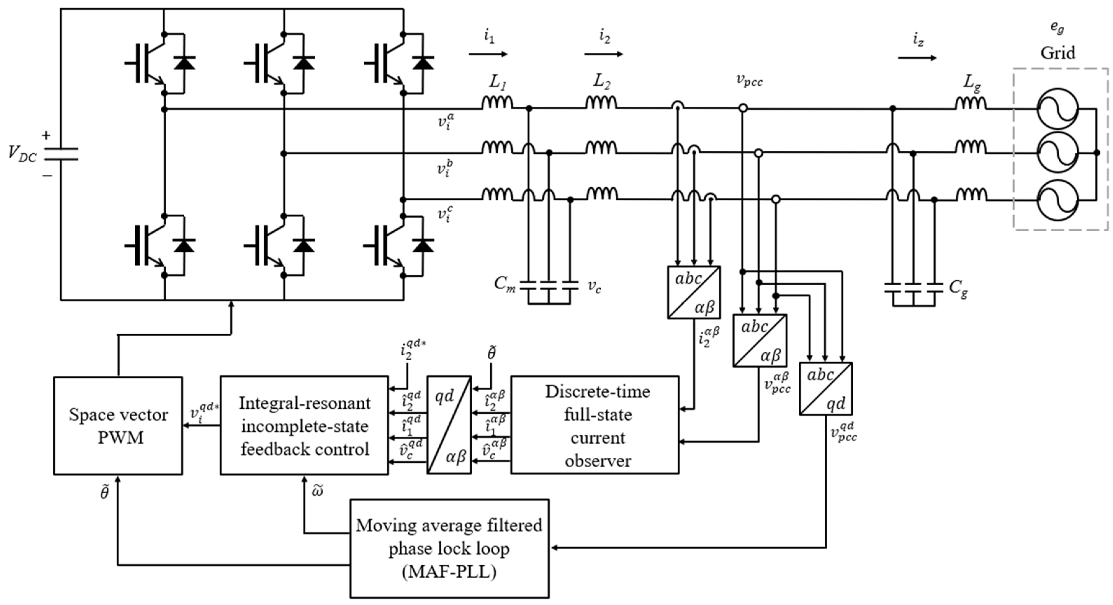
Figure 2.
Schematic of frequency detection based on the MAF-PLL.
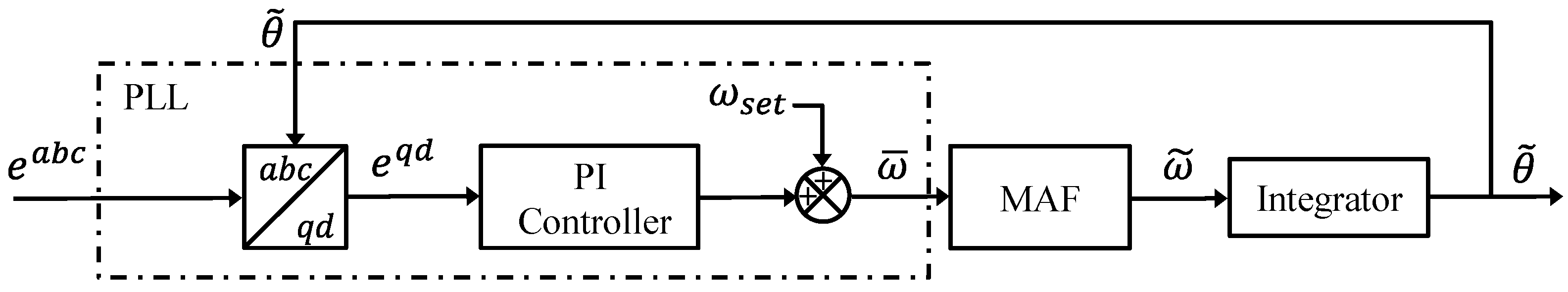
Figure 3.
Eigenvalues of the proposed control scheme. (a) Eigenvalues of ; (b) Eigenvalues of .
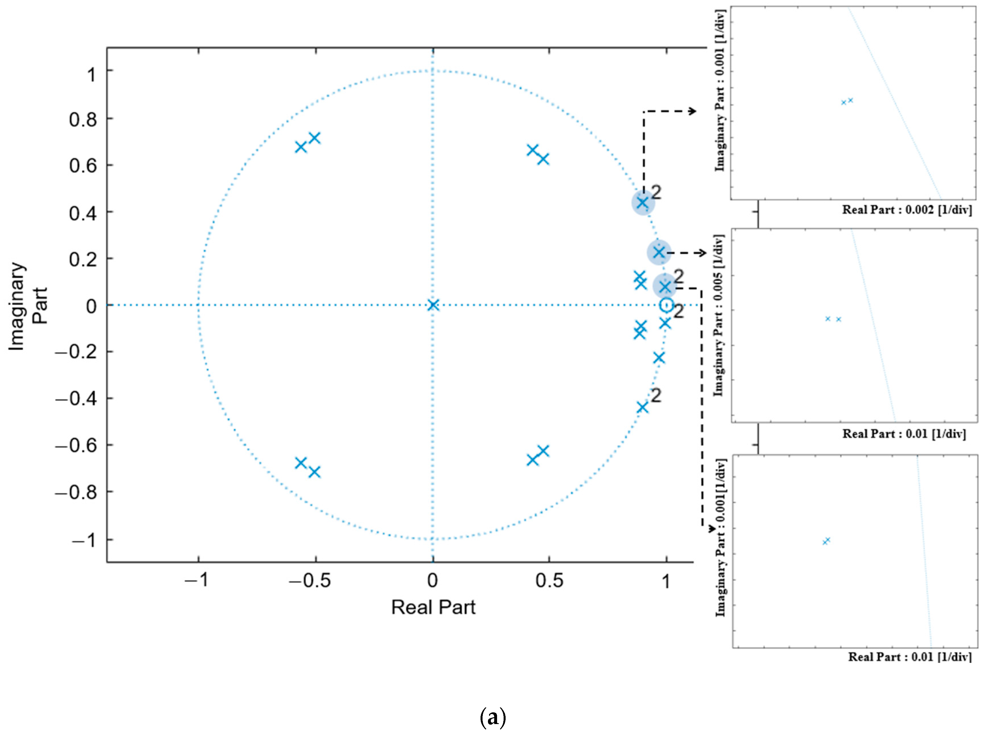
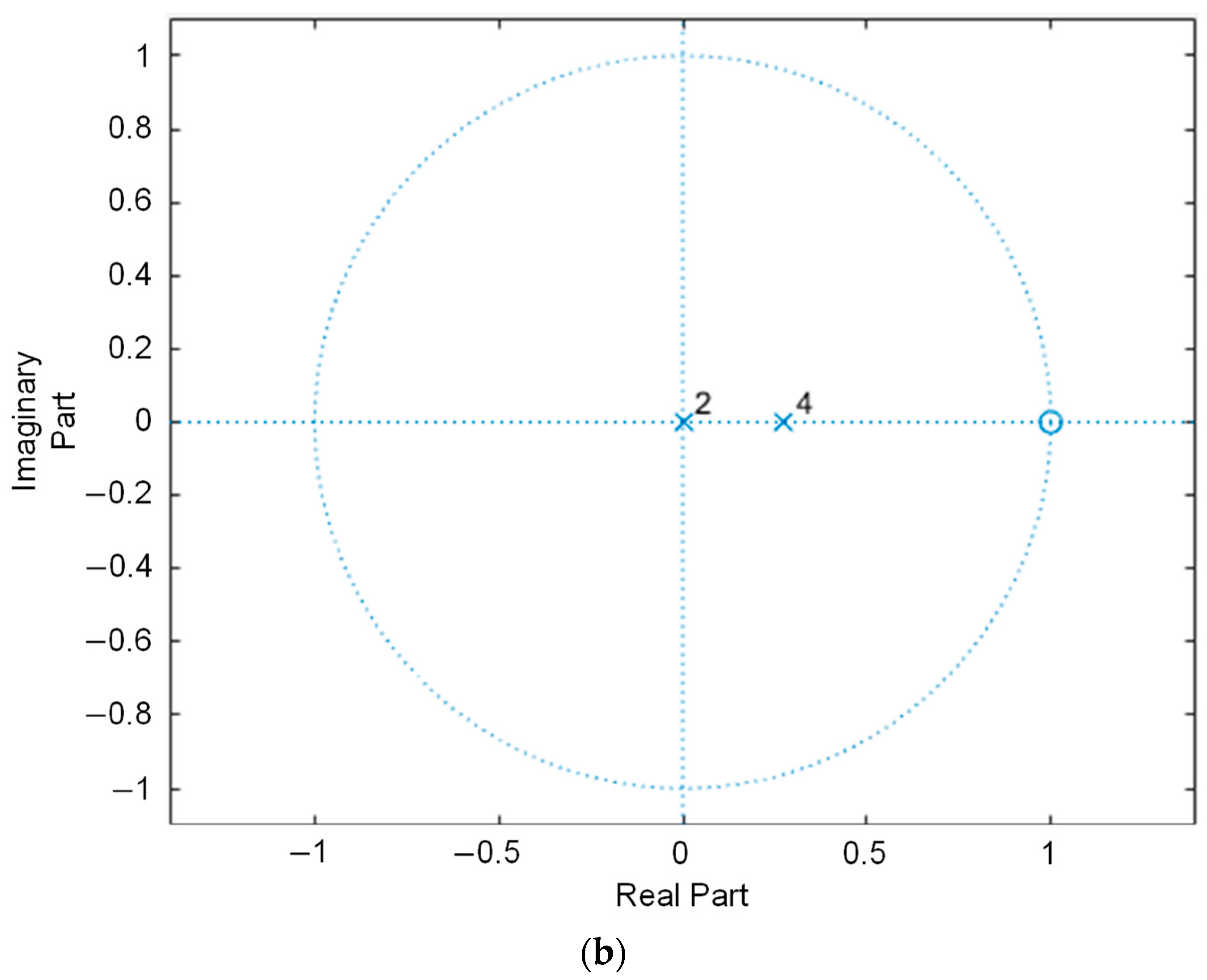
Figure 4.
Distorted and unbalanced grid voltages. (a) Voltage waveform; (b) FFT result of a-phase grid voltage.
Figure 4.
Distorted and unbalanced grid voltages. (a) Voltage waveform; (b) FFT result of a-phase grid voltage.
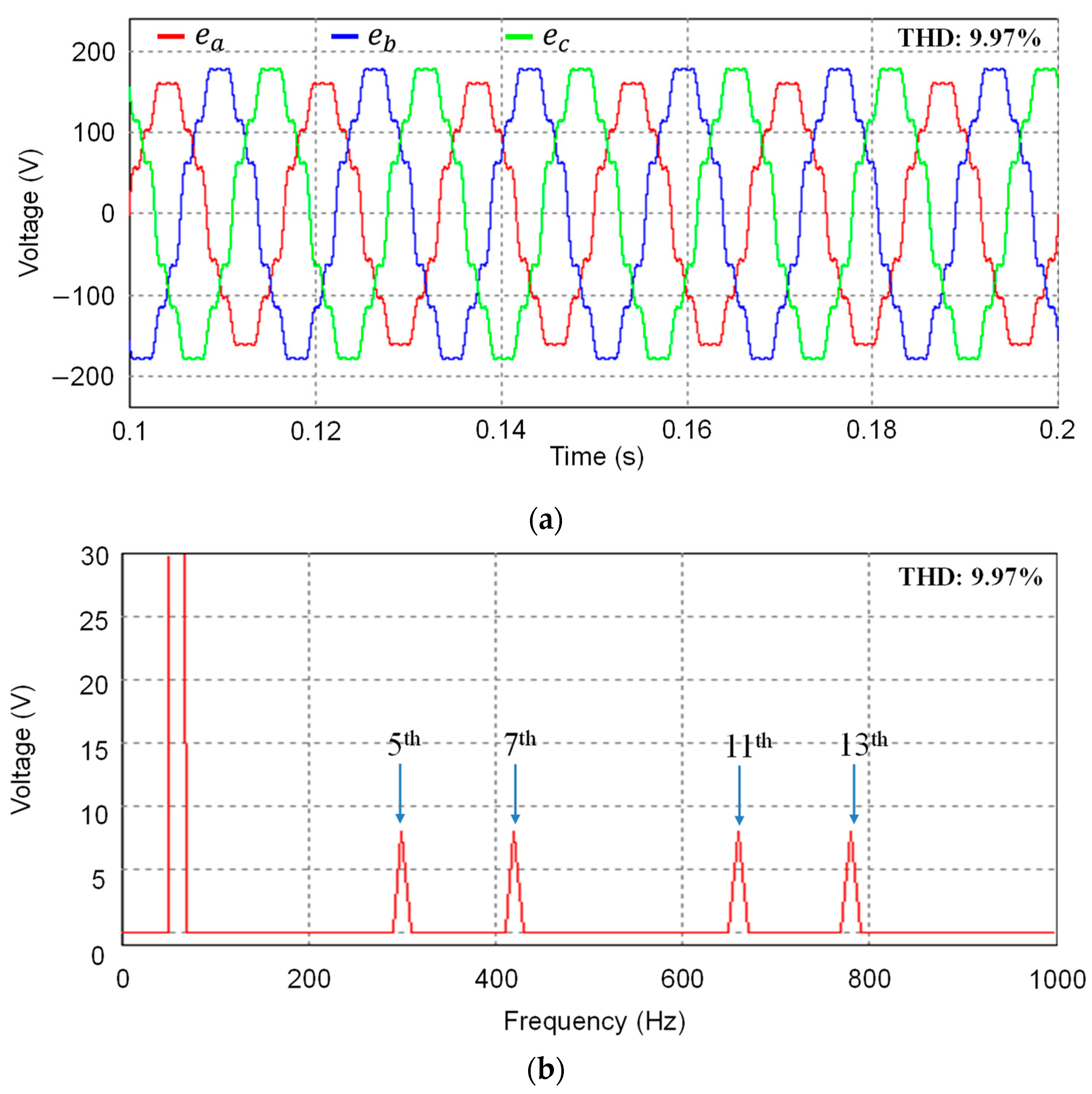
Figure 5.
Distorted and unbalanced PCC voltages. (a) Voltage waveform; (b) FFT result of a-phase PCC voltage.
Figure 5.
Distorted and unbalanced PCC voltages. (a) Voltage waveform; (b) FFT result of a-phase PCC voltage.
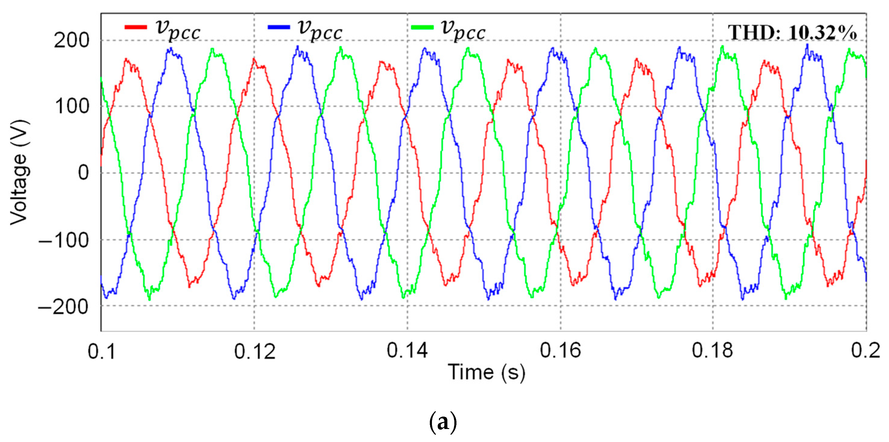
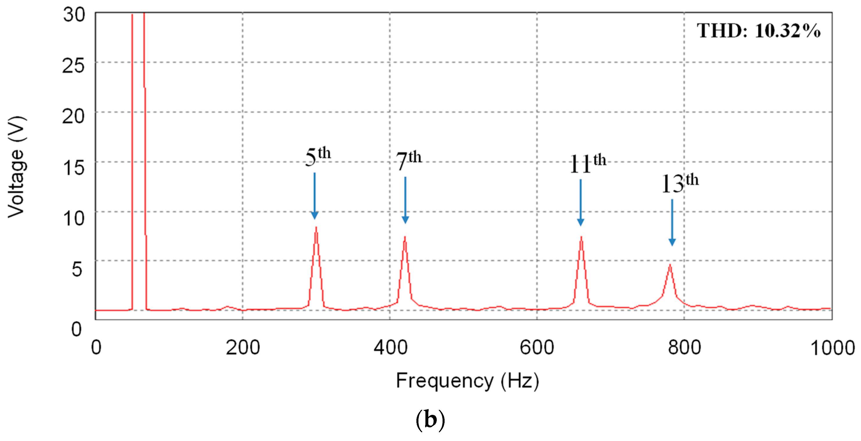
Figure 6.
Simulation results for the proposed control strategy at steady-state in the existence of unbalanced and distorted grid condition. (a) Grid-side current responses; (b) FFT result of a-phase current.
Figure 6.
Simulation results for the proposed control strategy at steady-state in the existence of unbalanced and distorted grid condition. (a) Grid-side current responses; (b) FFT result of a-phase current.
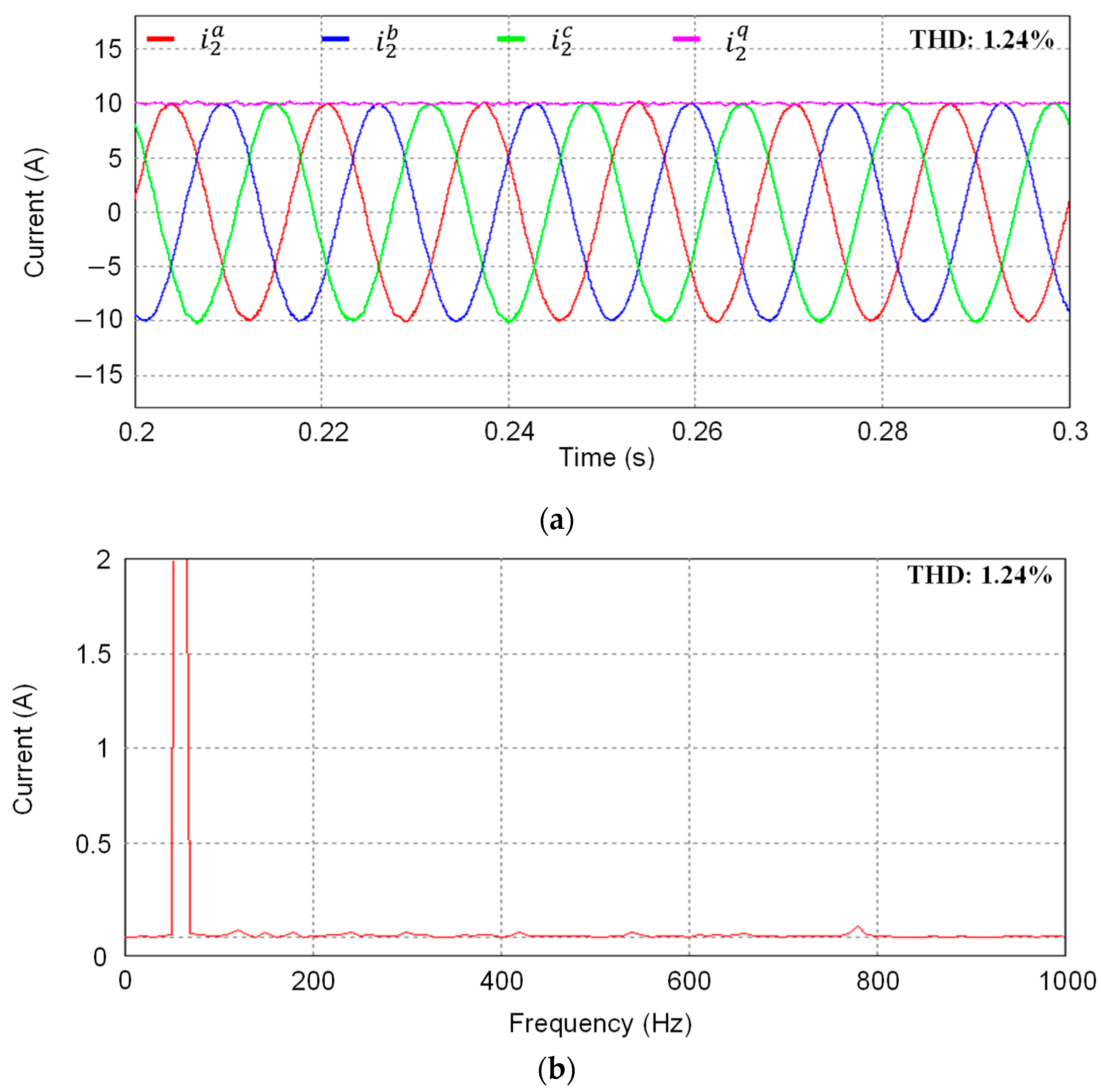
Figure 7.
Simulation results of transient responses for the proposed control strategy under unbalanced and distorted grid condition when the q-axis current reference has a step change at 0.25 s. (a) Grid-side currents; (b) Inverter-side currents; (c) Capacitor voltages.
Figure 7.
Simulation results of transient responses for the proposed control strategy under unbalanced and distorted grid condition when the q-axis current reference has a step change at 0.25 s. (a) Grid-side currents; (b) Inverter-side currents; (c) Capacitor voltages.
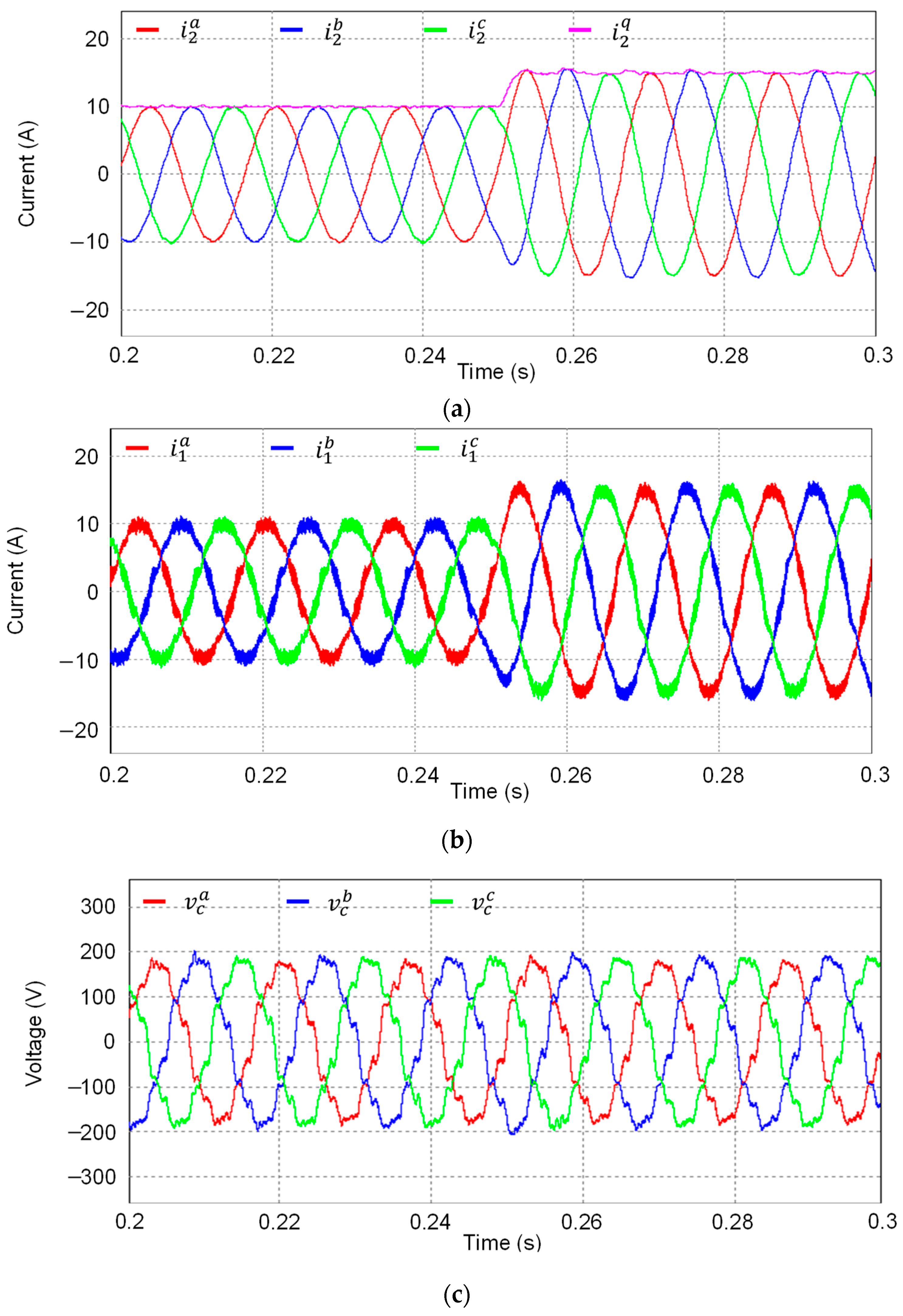
Figure 8.
Simulation results for the discrete-time current observer under the step change in q-axis current reference at 0.25 s. Sensed and estimated waveforms in the stationary reference frame. (a) Grid-side currents; (b) Inverter-side currents; (c) Capacitor voltages.
Figure 8.
Simulation results for the discrete-time current observer under the step change in q-axis current reference at 0.25 s. Sensed and estimated waveforms in the stationary reference frame. (a) Grid-side currents; (b) Inverter-side currents; (c) Capacitor voltages.
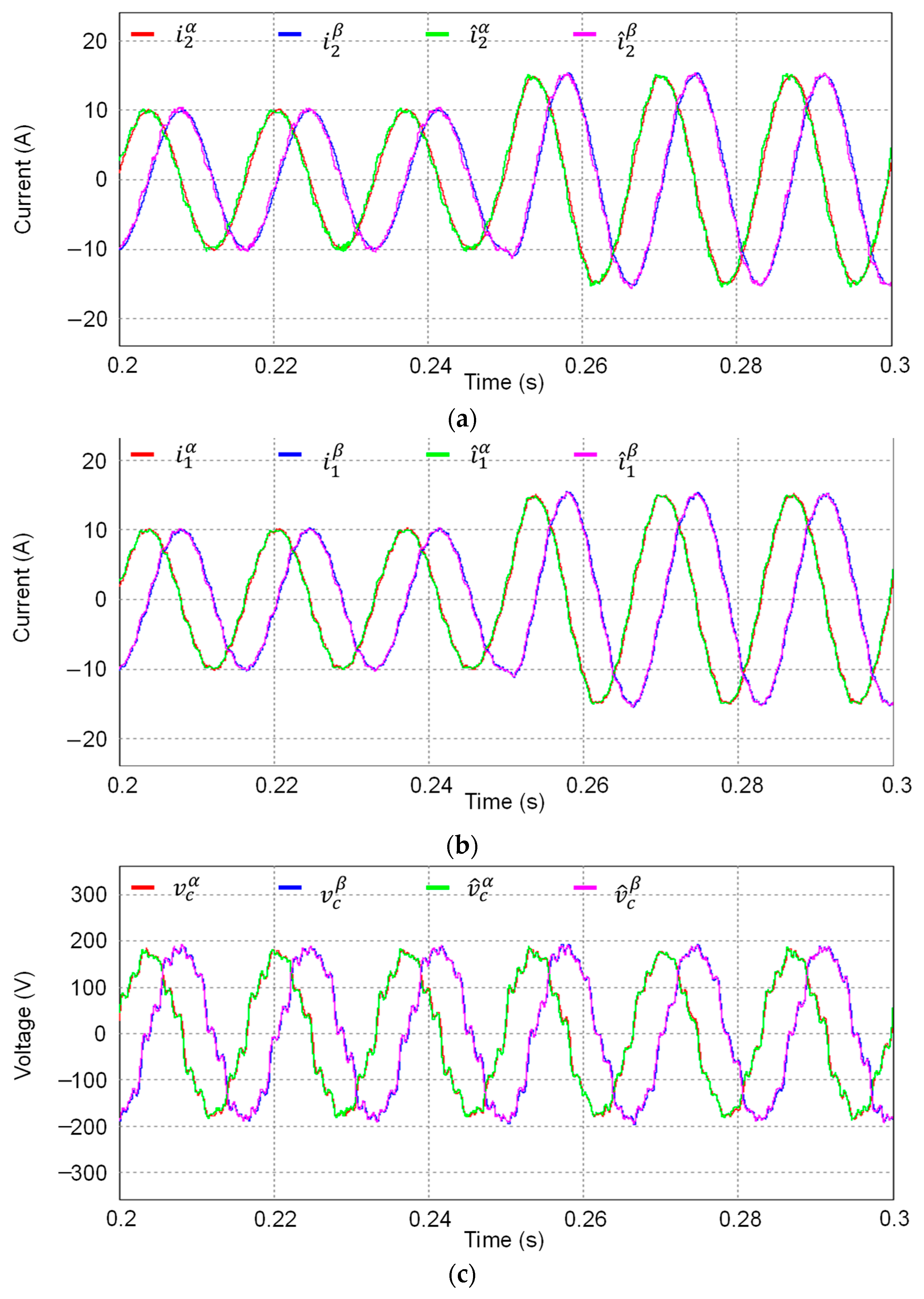
Figure 9.
Three-phase unbalanced and distorted grid voltages with frequency changes at 0.3 s and 0.4 s. (a) Grid voltages; (b) PCC voltages.
Figure 9.
Three-phase unbalanced and distorted grid voltages with frequency changes at 0.3 s and 0.4 s. (a) Grid voltages; (b) PCC voltages.
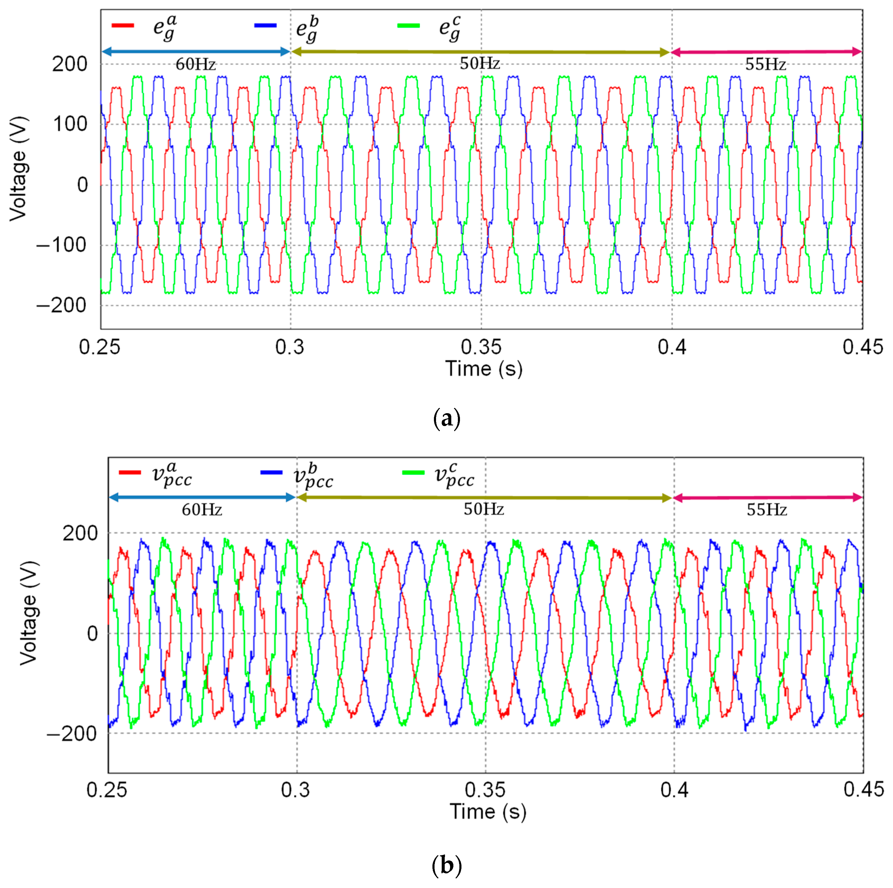
Figure 10.
Simulation results of the proposed control strategy under grid frequency changes at 0.3 s and 0.4 s. (a) Performance of frequency detection based on MAF-PLL; (b) Grid-side currents; (c) Inverter-side currents; (d) Capacitor voltages; (e) Enlarged waveform of grid-side currents at the instant of frequency change from 60 Hz to 50 Hz at 0.3 s; (f) Enlarged waveform of grid-side currents at the instant of frequency change from 50 Hz to 55 Hz at 0.4 s.
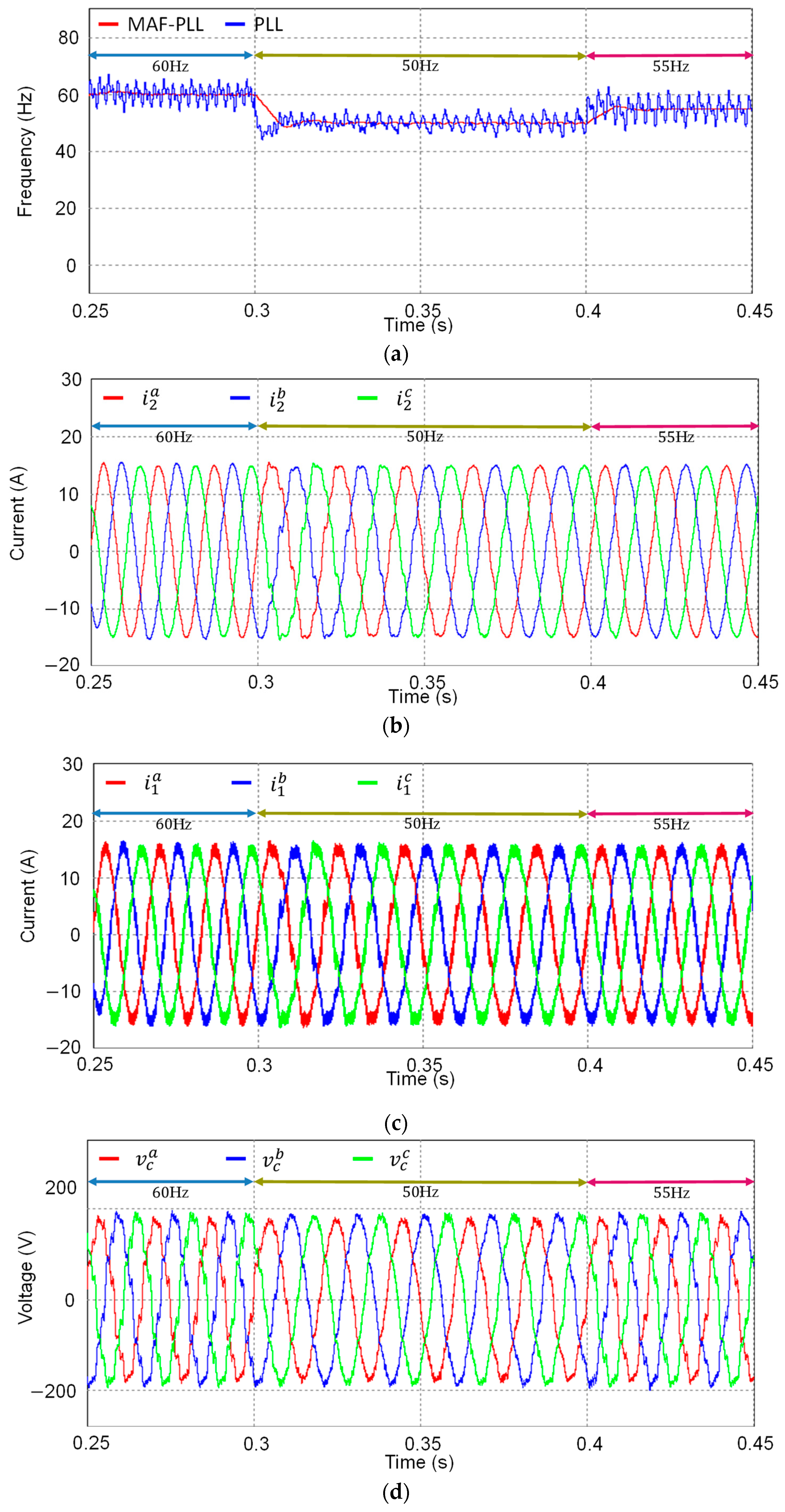
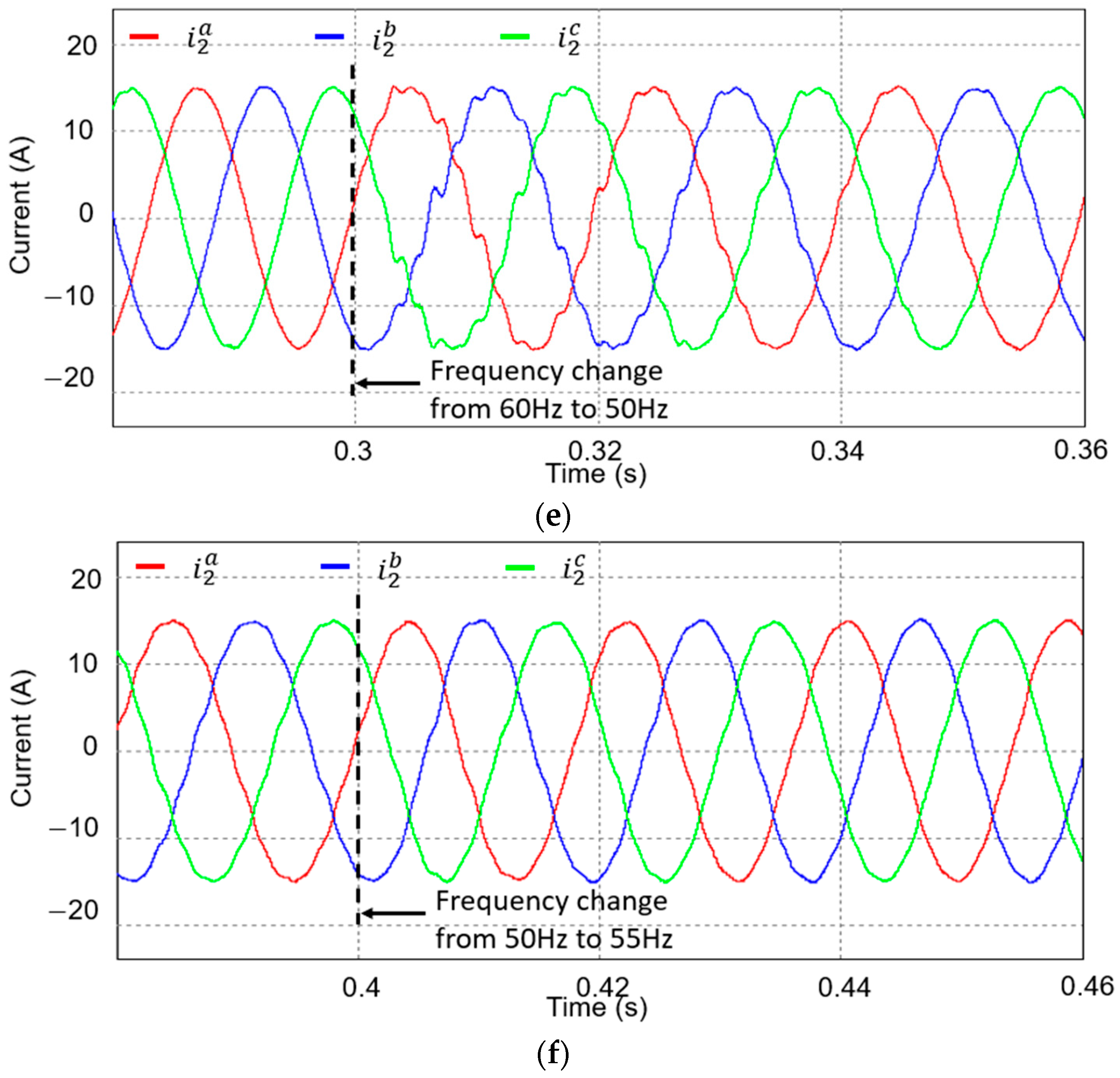
Figure 11.
Simulation results of the discrete-time current observer under grid frequency changes at 0.3 s and 0.4 s. Sensed and estimated waveforms in the stationary reference frame. (a) Grid-side currents; (b) Inverter-side currents; (c) Capacitor voltages.
Figure 11.
Simulation results of the discrete-time current observer under grid frequency changes at 0.3 s and 0.4 s. Sensed and estimated waveforms in the stationary reference frame. (a) Grid-side currents; (b) Inverter-side currents; (c) Capacitor voltages.
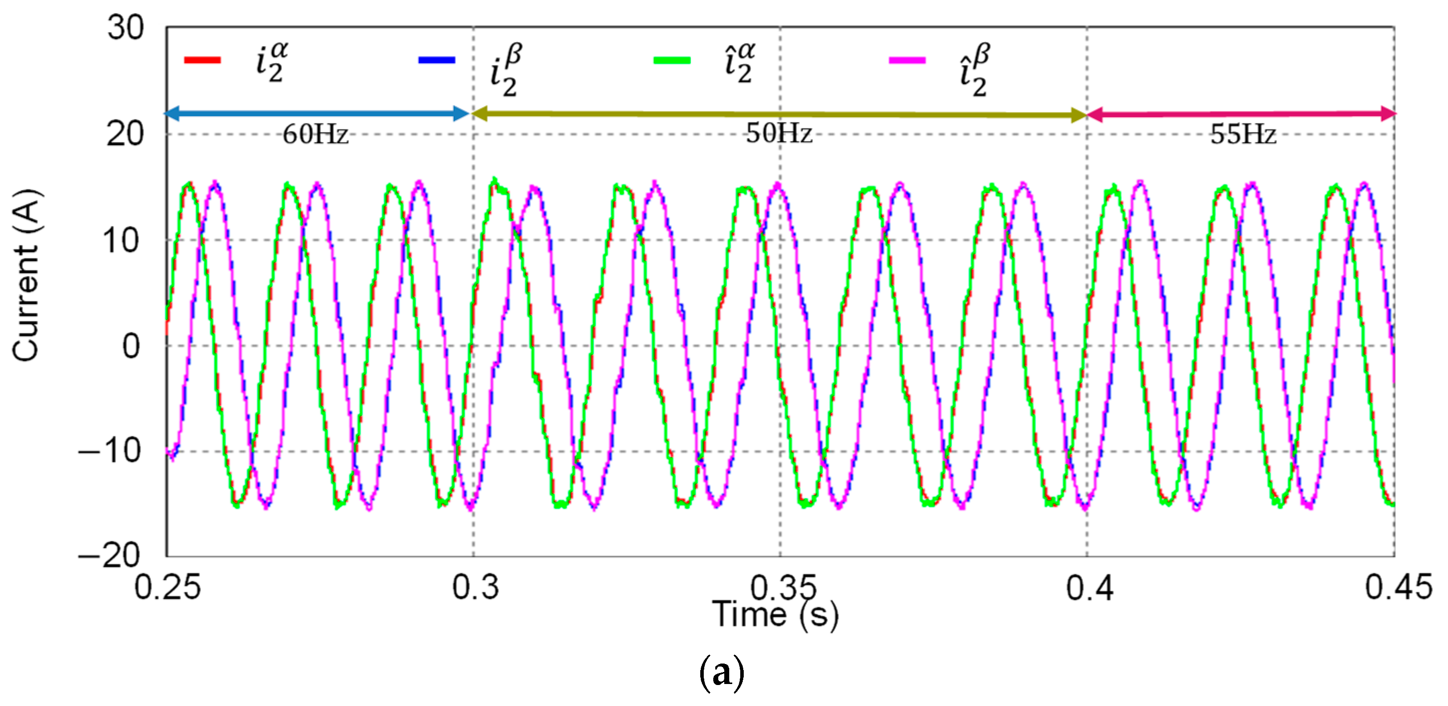
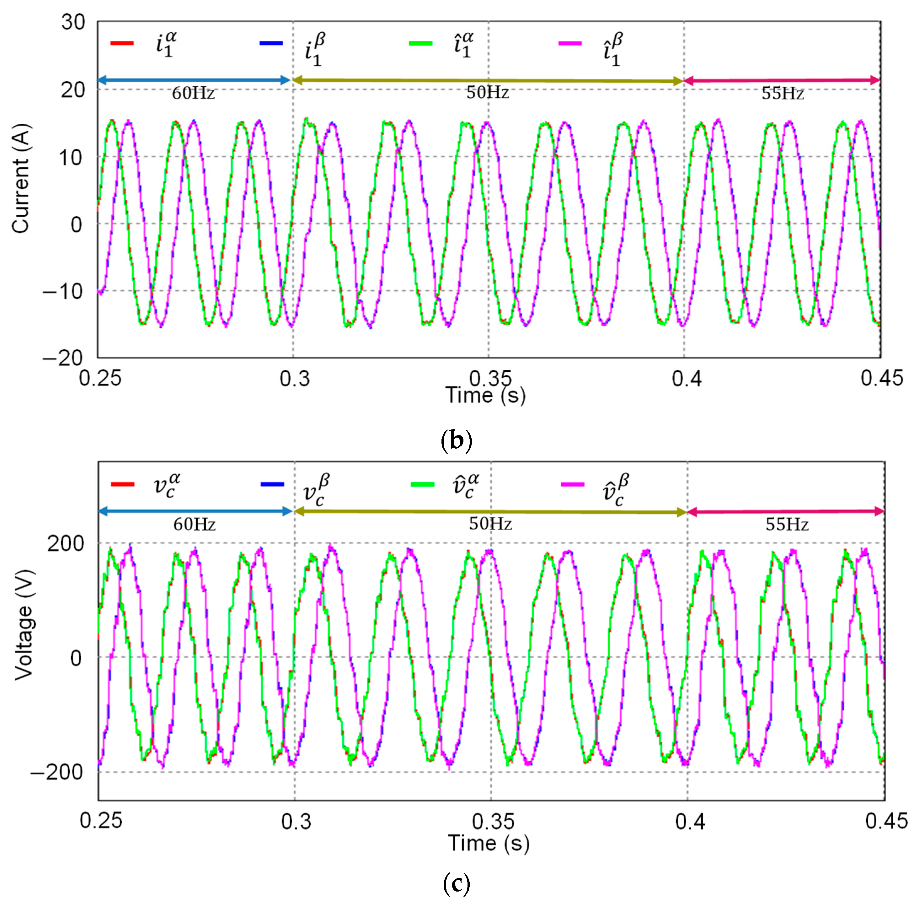
Figure 12.
Configuration of experimental system. (a) System configuration; (b) Photograph of experimental system.
Figure 12.
Configuration of experimental system. (a) System configuration; (b) Photograph of experimental system.
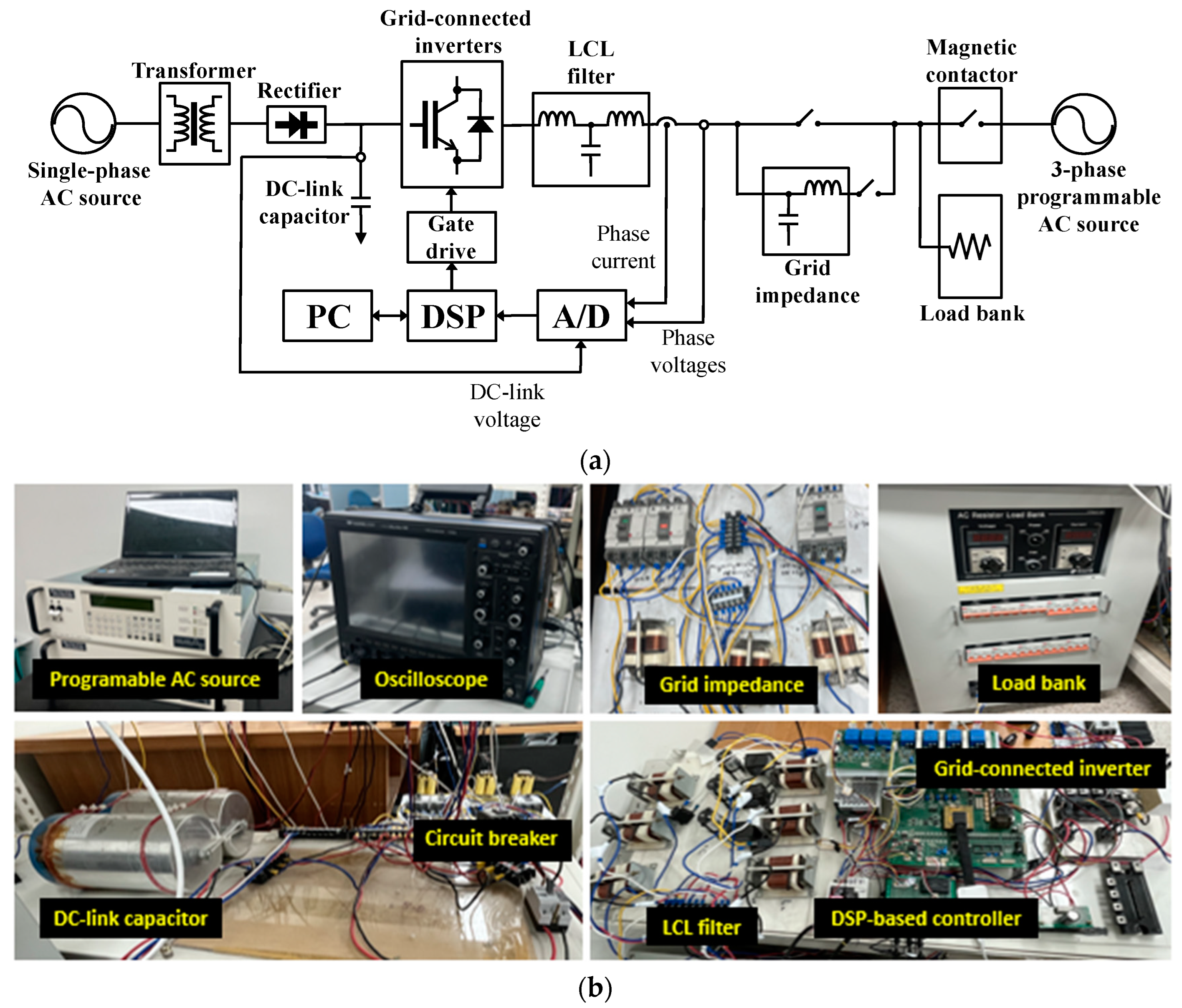
Figure 13.
Three-phase voltages for experiments. (a) Unbalanced and distorted grid voltages; (b) Unbalanced and distorted PCC; (c) FFT result of a-phase PCC voltage.
Figure 13.
Three-phase voltages for experiments. (a) Unbalanced and distorted grid voltages; (b) Unbalanced and distorted PCC; (c) FFT result of a-phase PCC voltage.
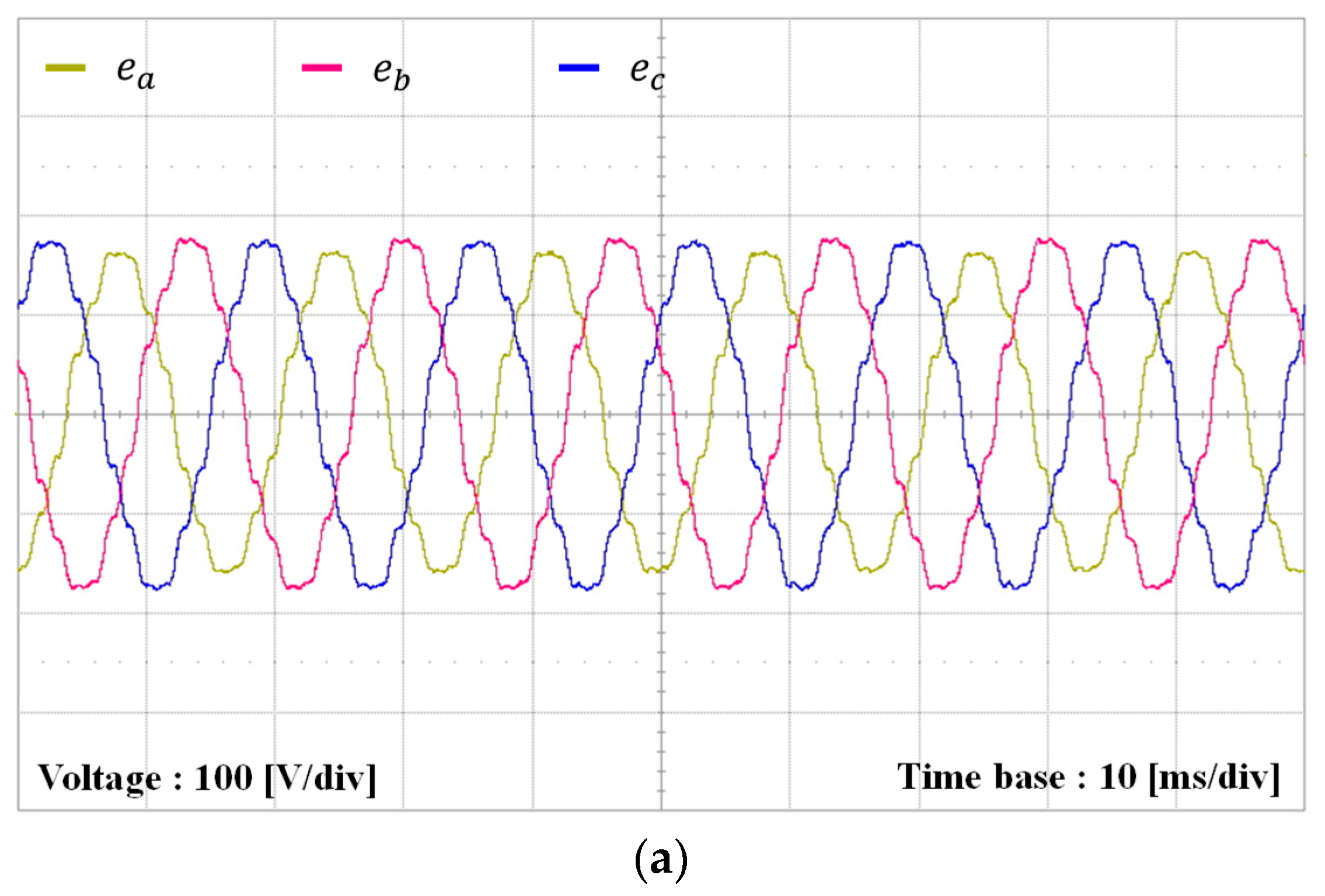
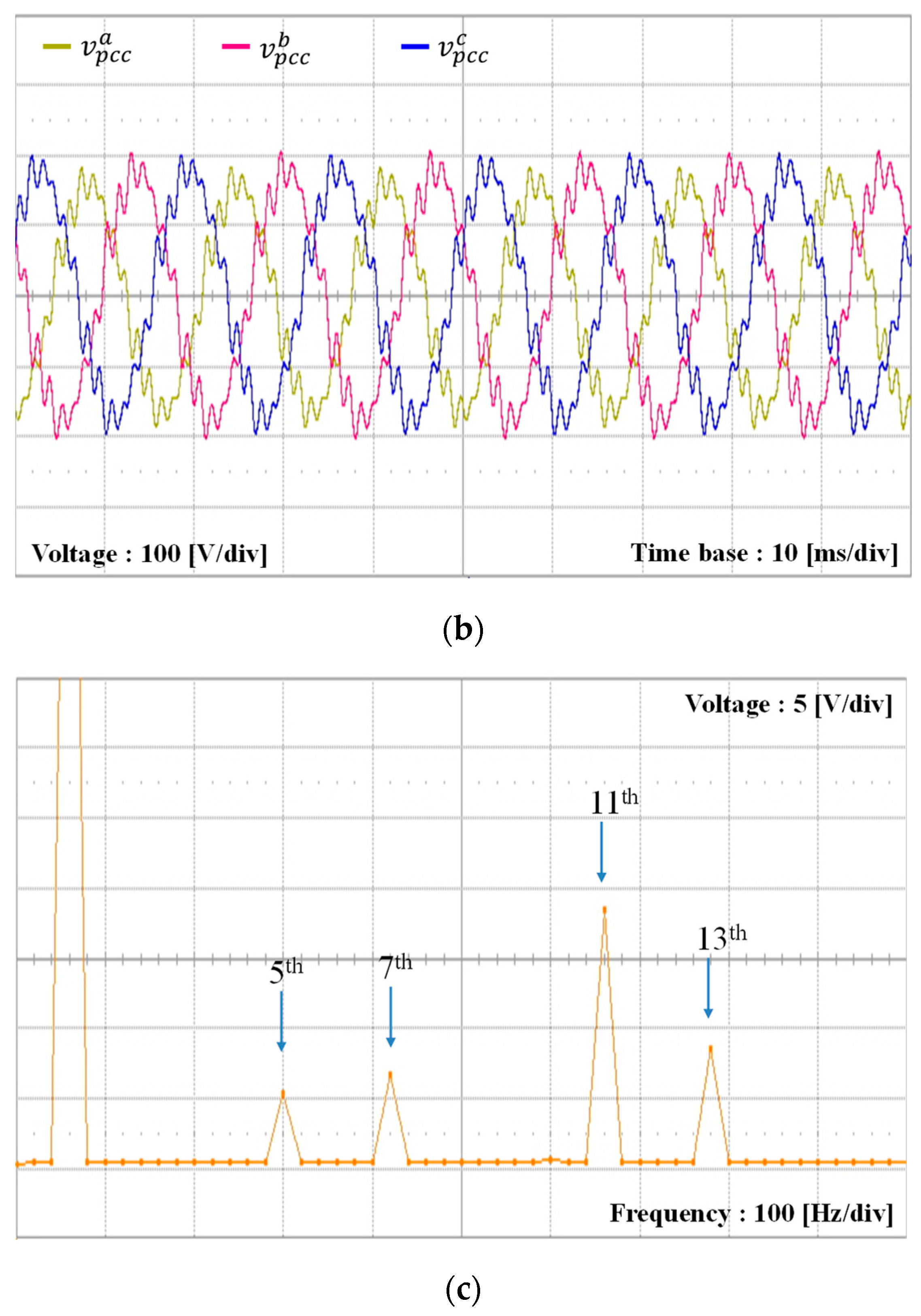
Figure 14.
Experimental results of the proposed control scheme at steady-state. (a) Grid-side current responses; (b) FFT result of a-phase current.
Figure 14.
Experimental results of the proposed control scheme at steady-state. (a) Grid-side current responses; (b) FFT result of a-phase current.
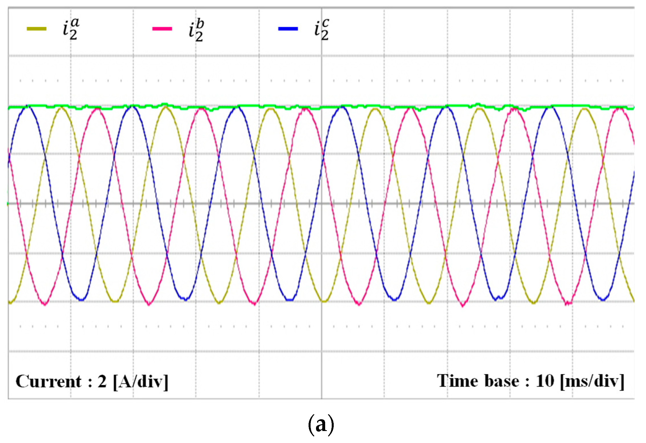
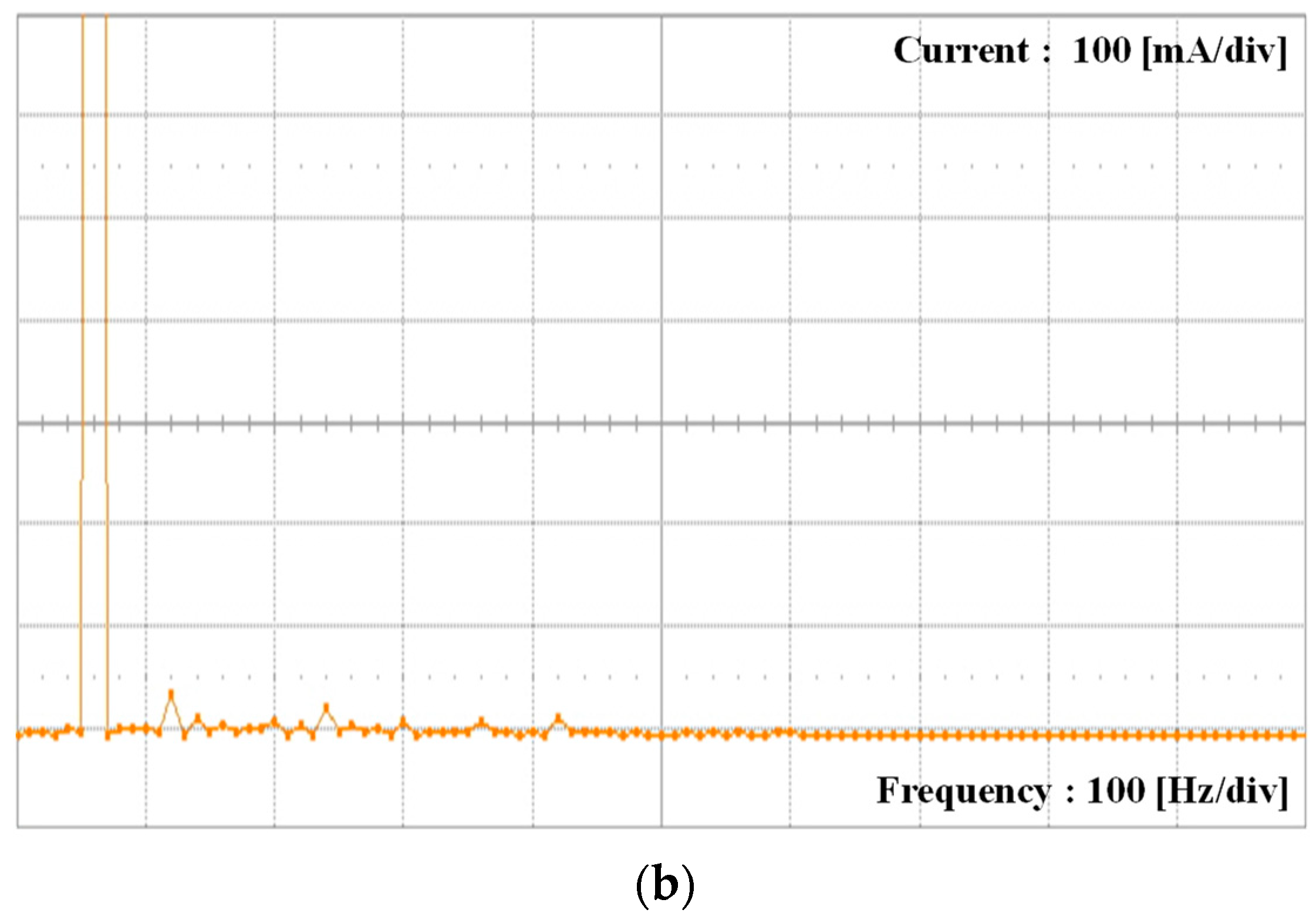
Figure 15.
Experimental results for transient responses of grid-side current with the step change of the q-axis current reference.
Figure 15.
Experimental results for transient responses of grid-side current with the step change of the q-axis current reference.
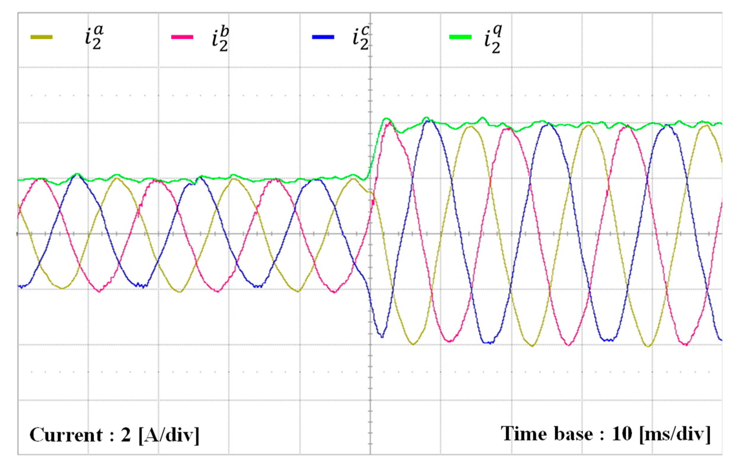
Figure 16.
Experimental results of discrete-time current observer with the step change in q-axis current reference. Sensed and estimated waveforms. (a) Grid-side currents; (b) Inverter-side currents; (c) Capacitor voltages.
Figure 16.
Experimental results of discrete-time current observer with the step change in q-axis current reference. Sensed and estimated waveforms. (a) Grid-side currents; (b) Inverter-side currents; (c) Capacitor voltages.
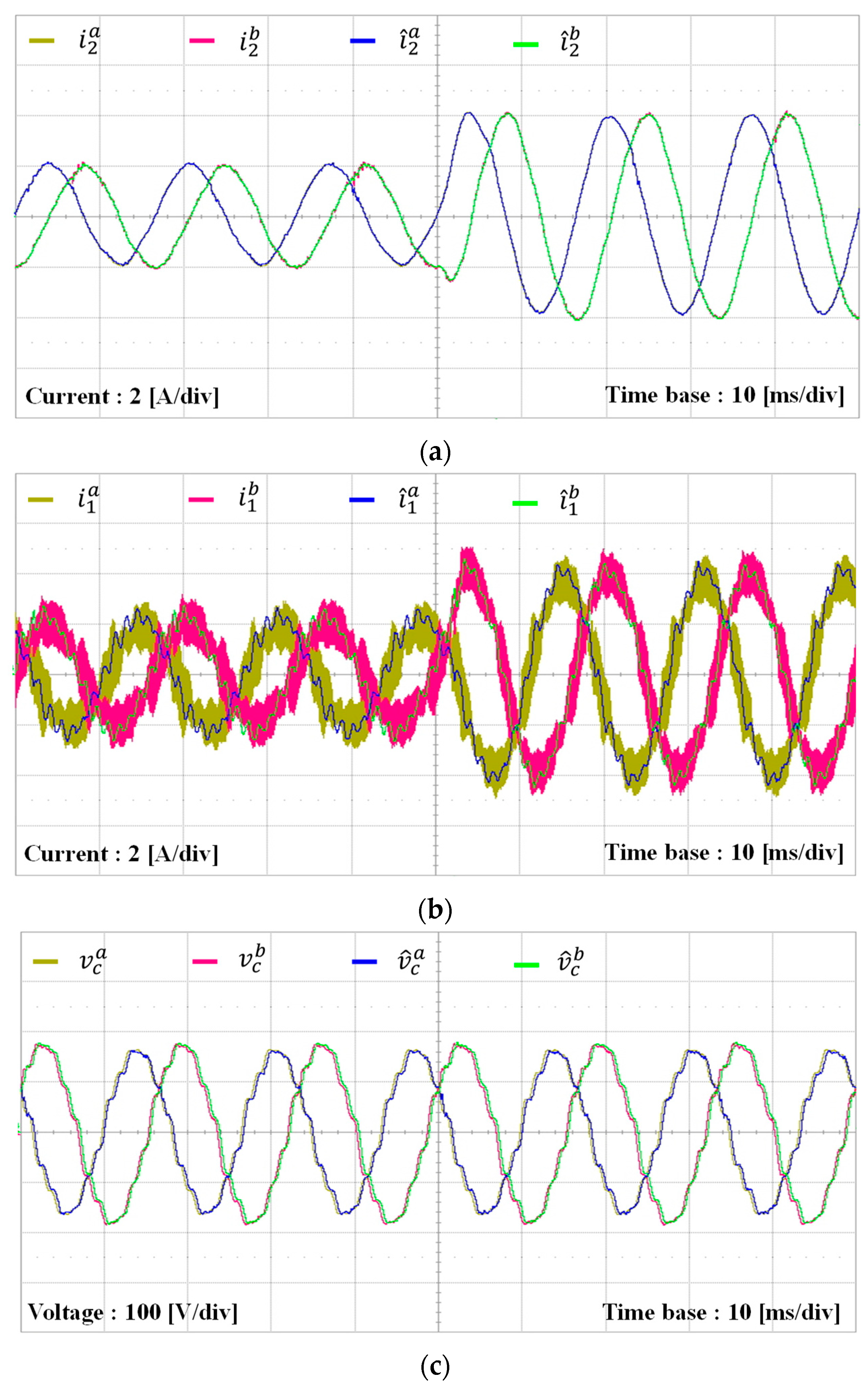
Figure 17.
Experimental three-phase unbalanced and distorted voltages during frequency change. (a) Grid voltages with frequency change from 60 Hz to 50 Hz; (b) PCC voltages with frequency change from 60 Hz to 50 Hz.
Figure 17.
Experimental three-phase unbalanced and distorted voltages during frequency change. (a) Grid voltages with frequency change from 60 Hz to 50 Hz; (b) PCC voltages with frequency change from 60 Hz to 50 Hz.
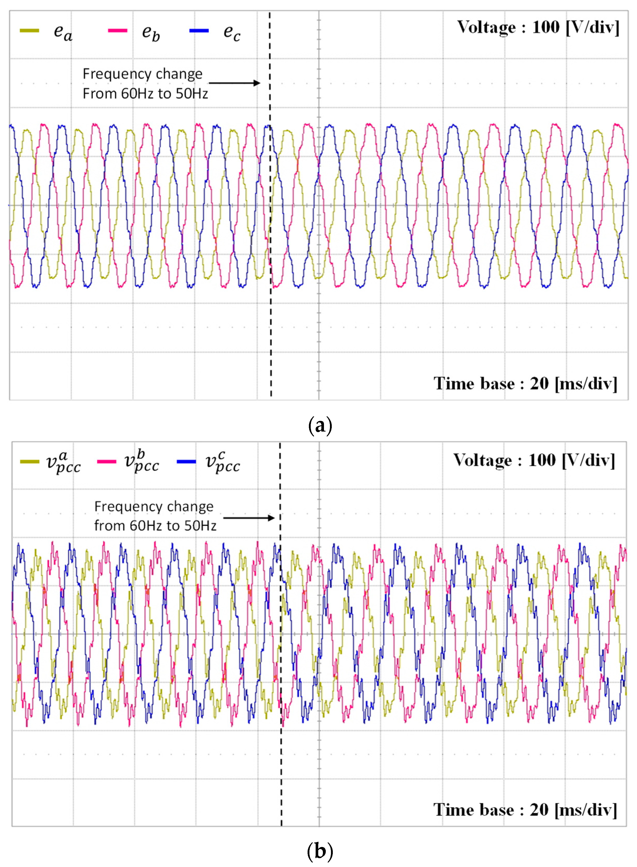
Figure 18.
Experimental results for transient response of grid-side current under frequency variation. (a) Transient responses of grid-side currents with frequency change from 60 Hz to 50 Hz; (b) Transient responses of grid-side currents with frequency change from 50 Hz to 55 Hz.
Figure 18.
Experimental results for transient response of grid-side current under frequency variation. (a) Transient responses of grid-side currents with frequency change from 60 Hz to 50 Hz; (b) Transient responses of grid-side currents with frequency change from 50 Hz to 55 Hz.
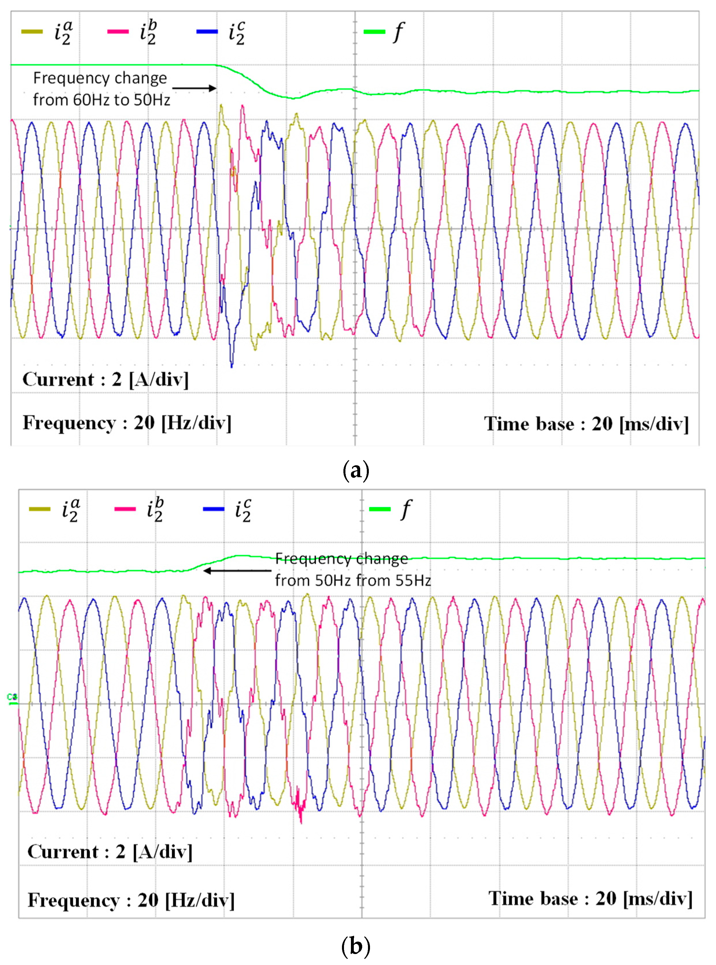
Figure 19.
Experimental results of discrete-time current observer with grid frequency change from 60 Hz to 50 Hz. Sensed and estimated waveforms. (a) Grid-side currents; (b) Inverter-side currents; (c) Capacitor voltages.
Figure 19.
Experimental results of discrete-time current observer with grid frequency change from 60 Hz to 50 Hz. Sensed and estimated waveforms. (a) Grid-side currents; (b) Inverter-side currents; (c) Capacitor voltages.
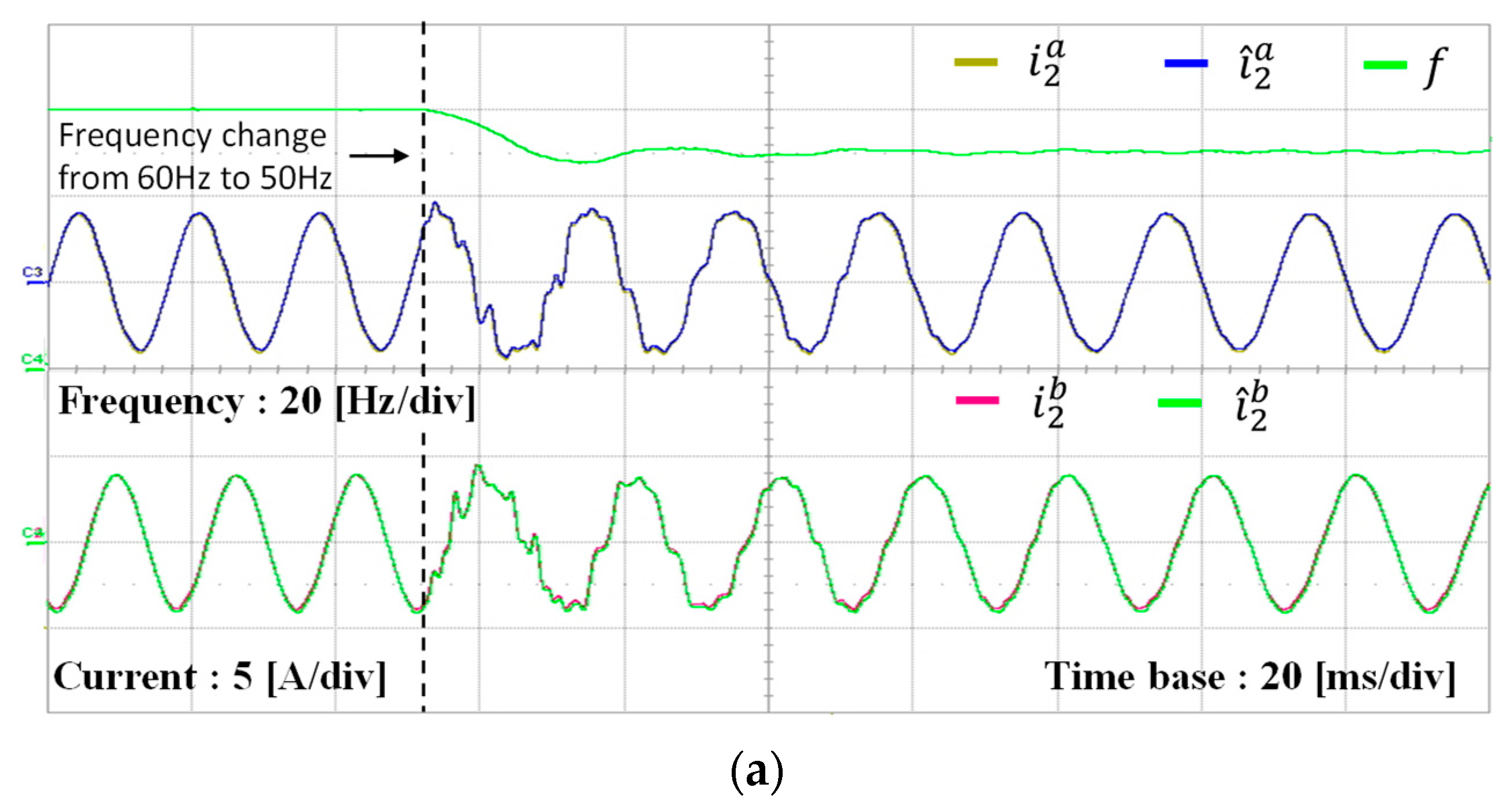
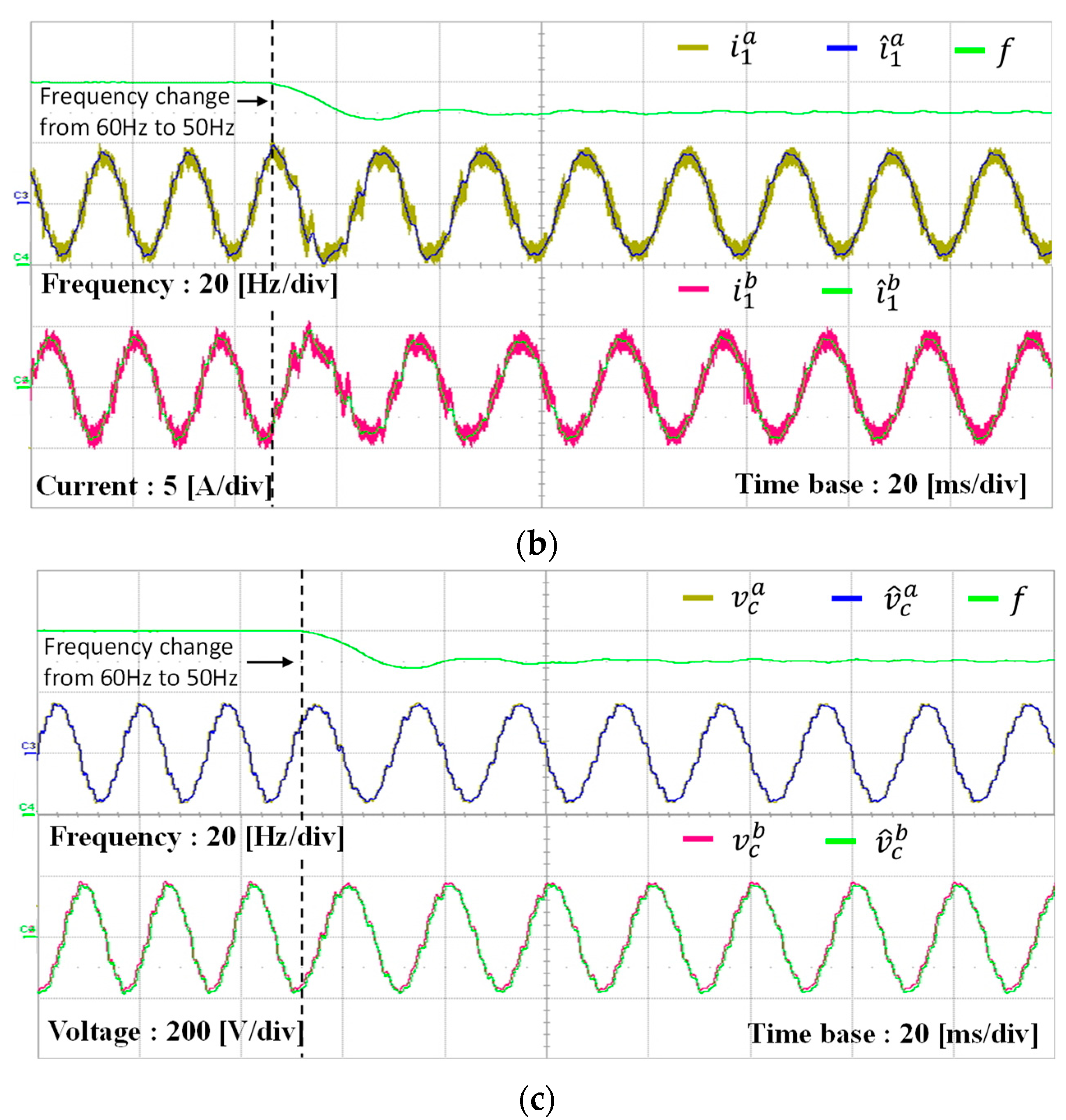
Figure 20.
Experimental results for discrete-time current observer under grid frequency change from 50 Hz to 55 Hz. Sensed and estimated waveforms. (a) Grid-side currents; (b) Inverter-side currents; (c) Capacitor voltages.
Figure 20.
Experimental results for discrete-time current observer under grid frequency change from 50 Hz to 55 Hz. Sensed and estimated waveforms. (a) Grid-side currents; (b) Inverter-side currents; (c) Capacitor voltages.
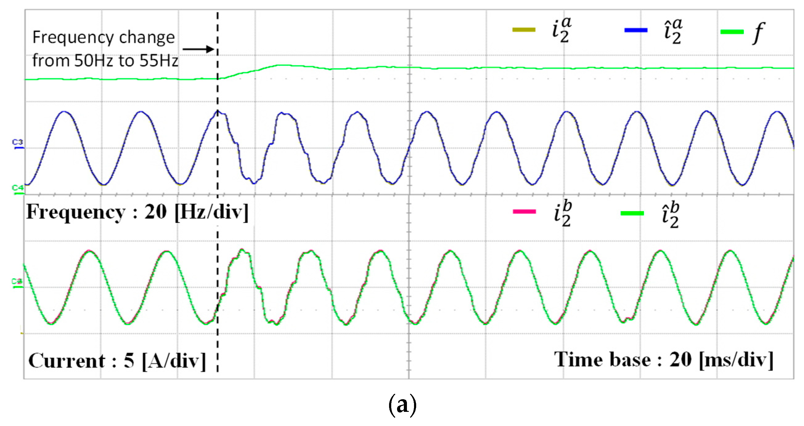
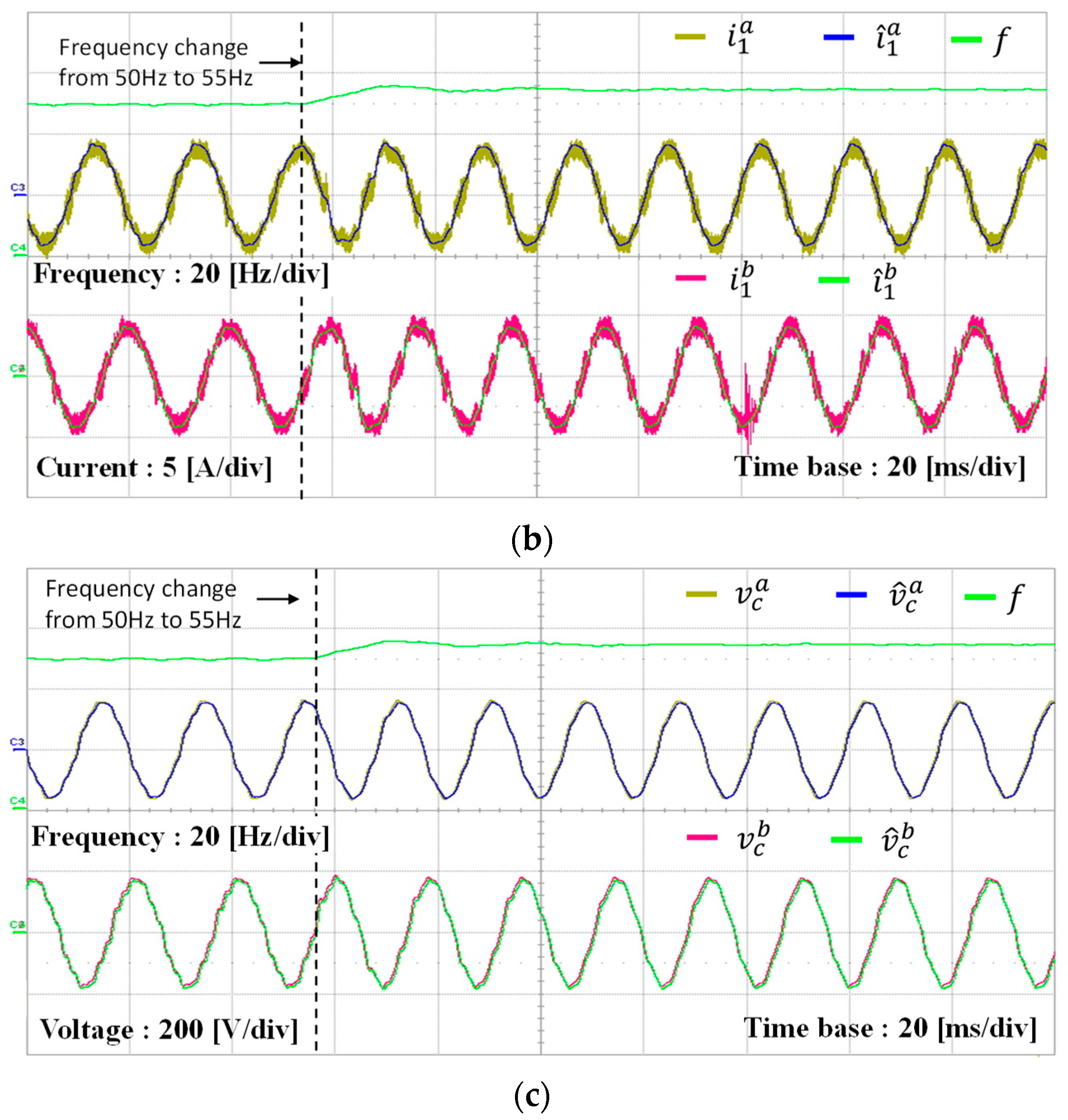

Table 1.
Parameters of a GCI system.
| Parameters | Value | Units |
|---|---|---|
| DC-link voltage | 420 | V |
| Grid voltage (line-to-neutral) | 180 | V |
| Grid frequency | 60 / 50 / 55 | Hz |
| Grid capacitance | 6 | µF |
| Grid inductance | 3 | mH |
| Grid-side filter inductance | 0.9 | mH |
| Inverter-side filter inductance | 1.7 | mH |
| Filter capacitance | 4.5 | µF |
Disclaimer/Publisher’s Note: The statements, opinions and data contained in all publications are solely those of the individual author(s) and contributor(s) and not of MDPI and/or the editor(s). MDPI and/or the editor(s) disclaim responsibility for any injury to people or property resulting from any ideas, methods, instructions or products referred to in the content. |
© 2025 by the authors. Licensee MDPI, Basel, Switzerland. This article is an open access article distributed under the terms and conditions of the Creative Commons Attribution (CC BY) license (http://creativecommons.org/licenses/by/4.0/).
Copyright: This open access article is published under a Creative Commons CC BY 4.0 license, which permit the free download, distribution, and reuse, provided that the author and preprint are cited in any reuse.


