Submitted:
26 February 2025
Posted:
27 February 2025
You are already at the latest version
Abstract
Lie scale invariance is used to reduce the incompressible Navier-Stokes equations to non-linear ordinary equations. This yields a formulation in terms of logarithmic spirals as independent variables. We give the equations when the spirals lie on cones as well as in planes. The theory gives a locus in cylindrical coordinates of singularities as they arise in the reduced Navier-Stokes equations. We give two formal examples aimed at discovering singularities in the flow; another example is related to a Hele-Shaw cell, and finally we explore the flow through propellers comprised of blades made from congruent logarithmic spirals.
Keywords:
Lie symmetry
; fluids
; singularities
; Hele-Shaw cell
; propellers
1. Introduction
The implications of the Navier-Stokes equations as a function of scale is a famous problem. Applications normally appear in the theory of turbulence [1,2]. One way of proceeding is to translate these equations into a self-similar, that is a scale independent form. We do this following the Lie formalism described in [3] and elaborated in [4].
In this paper we are restricted to incompressible, viscous flow, which has a viscosity largely determined by the scale invariant requirement. The Lie symmetry is taken to be in the radial direction in this paper. An alternate, but parallel, discussion would take the Lie symmetry to be in the axial (z) direction.
Our scale invariant variable represents an expansion of the flow in terms of equiangular (i.e logarithmic) spirals at different times. A flow of this type, free of controlling surfaces, would be subject to a two point boundary condition in angle. With external controls, a boundary condition would be applied on one of these spirals made into a real surface. In such a case our study with radial inflow has some resemblance to the inverse sprinkler problem [5]. We use it here to investigate the locus of singularities in cylindrical coordinates, to study flat Hele-Shaw type flows, and equi-angular propellers. The latter example requires the logarithmic spirals to lie on cones rather than in a plane. This will be our major example.
The cylindrically symmetric, time dependent, limit (when the spirals are circles) may be solved analytically, as can a similar model in the Euler equations. The singularity structure, or the lack of it, may be seen at all scales in these examples.
This is a purely formal result, but a very approximate conceptual model of such flow is shallow water exiting through a circular pipe out of a surrounding circular reservoir. The fluid must have been given some initial angular momentum about the pipe axis. We have added angular dependence in the Euler example without viscosity.
We have also investigated numerically more general versions of our scale invariant equations elsewhere. Singularities occur frequently on logarithmic spirals, and there are unexpected reversals of the sign of angular momentum as a function of (see also [6]).
In the next section we introduce the technique. The resultant formulation of the Navier-Stokes equations is the principal result of this paper. The Subsequent sections describe examples of some physical interest, and also of some mathematical interest regarding singularities in the equations.
2. Scale Invariant Variables
By ‘scale invariant variables’ we refer particularly to the formalism introduced in [3] and at length in [4].
We take the Navier-Stokes equations to be
where the vorticity and the sum of the thermal, kinetic and potential energies are
The external potential V can be included only if it happens to fit the scale invariant functional form. The fluid velocity is represented by , the pressure is p and the constant density is .
In this paper we use a Lie symmetry in radius (we refer to a cylindrical coordinate system ), according to
because, for any length, the dimensional co-vector is 1. The parameter T depends only on r. The quantity is a reciprocal length scale that can be chosen at will to study different scales in the flow.
Along this radial scaling motion we must have (the angle is discussed below) for complete consistency
where [4] and are invariant under the scale change. That is they can not depend on T (i.e. r), but rather only on some combination of variables that is also invariant. The quantity is another reciprocal length scale dedicated to the Lie scaling in time.
For example according to equations (3) and (4), . The total derivative of with respect to r must be zero which requires .
We do not allow a full variable dependence in this paper, because this would double the independent variables. It appears in our equations through a scale invariant variable (see e.g. equation (11 below), but has to be set subsequently to an arbitrary constant value in the equations to avoid breaking the symmetry . We shall see below that the variable , when set equal to a constant, describes a conical surface bearing equi-angular spirals, where the exterior conical angle is given by .
Allowing the local time to scale with radius as indicated in equation (4), also breaks the radial Lie symmetry by introducing into the equations. Holding constant (as we do with when present) would imply looking at different radii at different times, just as holding constant implies different z at different radii. Instead, we can replace the local time scaling in equation (4) with a global time scaling that is independent of radius or azimuth. We give this global definition of below. This strictly contradicts the assumed Lie symmetry. However it turns out that in one particular case (), the equations admit a global, intrinsic, time scale. For the Euler equations, the intrinsic time scale is replaced by an external time scale but remains zero. The more general case, classified by is restricted to the steady state.
We keep the arbitrary reciprocal scales explicitly. In effect they vary our resolution of the flow as a kind of mathematical `loupe’. It happens that scale invariant solutions of mechanical systems depend on the ratio of the reciprocal spatio/temporal scales, which ratio we designate by
and which is elsewhere referred to as the similarity class [3], [4].
The scale invariant angle (i.e. the total radial derivative of is constant) is defined [3] as ( is an arbitrary rotation rate along the Lie scaling direction)
but we will use it multiplied by an arbitrary constant in the form
Here, is another arbitrary constant that absorbs .
The same scaling symmetry is applied to the dependent quantities , and the kinematic viscosity , we follow the dimensional prescription for the variation along the Lie motion in r to write them as
where , and are now scale invariant quantities. The quantity is a place holder for the combined scale invariant variable that we define below. Equations (1) are to be expressed in terms of these quantities.
Technically, although this is not the subject of this paper, we have used use variable reciprocal scales, and to form the space-time reciprocal dimensional vector (corresponding in position to space and time) . This forms a dot product with a (quantity dependent) numerical co-vector , which corresponds in position and sign to the number of spatial and temporal dimensions of the quantity of interest. The dot product gives the factor by which a quantity changes exponentially along a Lie scaling motion [3]),[4], namely . Here the differential (not to be confused with ) is an increment along the Lie symmetry direction. Thus we have , because is constant along the Lie motion.
Similarly
The expression for is naturally part of the description of an incompressible, scaled fluid; but the scaling form for the external potential is a severe constraint. Subsequently we will not include the potential explicitly; but it can be included through summed with , if it is compatible with the assumed symmetry.
Provided that the kinematic fluid viscosity in equation (8) is constrained by requiring to be a global constant (i.e. independent of ), we can define a global scaled time as
Here is a dimensionless constant, whose value allows some external forcing. For the Euler equations, we will use where is an externally applied reciprocal time. The spatial scaling implied by the constant , allows the viscous global time scale to vary with an arbitrary length scale. The fixed time at any spatial scale removes any additional temporal scaling of the system [3]. Hence we will require (and hence ), whenever the flow is not steady.
The three independent scale invariant quantities ,, and can be used in principle to express equations (1), rather than using . This removes r from the independent variables [3], but leaves a multi-variable problem even in the steady state.
To proceed more simply, we look for solutions of a single combined scale invariant variable, . We choose a sum of the individual invariants , and . In principle might be any function of the scale invariants, but such a choice is not guaranteed to eliminate all of coordinates from the equations.
The sum of , and defines a spiral basis through (we use the global definition of )
The quantity allows for some external forcing instead of the viscous decay. In the Euler limit, the time dependence is simply , where has the dimension of reciprocal time and might be an applied frequency.
We allow the constants (and when applicable and ) to be positive or negative. In general, the solutions are single valued only over an interval of the combined variable .
Although we do not consider a self-gravitating fluid in this paper it is useful to consider such an example to show the physical significance of the index a. We assume for this purpose an axially symmetric, steady, () cylindrical distribution of mass. We take a power law (scale invariant) density distribution . This produces a self gravitational potential ( for a bound system)
which for compatibility with the scale invariant form should equal
Consequently, we must have W to be constant and . When , and there is no line mass at the centre, we require and with and . Note that in this case.
Despite this illustrative toy example; in this paper, for incompressibility, and an applied potential is not explicitly discussed. The index a is therefore not constrained in a steady state.
3. Navier-Stokes Equations as Ordinary Equations
3.1. Steady State
We substitute the expressions (8), (4) and (9) together with the definition of (11) into equations (1). We write the steady equations with and keep the similarity class a general. We find (the prime indicates the derivative with respect to as defined in equation(15) the following scale invariant equations;
The incompressible condition,
When , our equations apply only where . In strict cylindrical symmetry . In the steady state the independent variable (see 11) is,
It is convenient to introduce a velocity along the vector (perpendicular to the surface of constant ) as
and
We may use the continuity equation to eliminate in favor of whenever and
The azimuthal velocity is then given in terms of , and by
These expressions are also simplified if (when viscosity is uniform), because then equation (18) can be integrated.
The radial component of the Navier-Stokes equation becomes (we show an example of the necessary algebra in an Appendix),
The azimuthal component of the Navier-Stokes equation,
The longitudinal component of the Navier-Stokes equation,
Should , the viscosity is constant in space and time. The value implies that velocities (and energies) are constant under the Lie motion in radius. It is usually termed `homothetic’. Other values of a correspond to constants with other dimensions. For example , that is , corresponds to a constant acceleration under the Lie motion in radius. The value implies a velocity that scales like , while implies the Kolmogorov velocity scaling .
Appendix A gives the derivation of equation (20) as an example of the necessary algebra.
3.2. Time Dependence
When so that time dependence is possible, we must take and . The Lie invariant becomes ( recall )
This gives the flow equations (plus the continuity equation 14) as:
Radial equation;
Azimuthal equation;
Longitudinal equation;
For completeness we proceed next to the zero viscosity Euler equations under this formulation.
3.3. Euler Equations
We obtain the Euler equations under this symmetry by setting in the equations of the preceding steady state section, except on the left side of each equation when there is time dependence. In that case we replace on the left with , and so that has the dimension of reciprocal time.
The Euler equations become explicitly (plus equation 14) for the steady state:
Radial equation;
Azimuth equation;
Longitudinal equation;
The continuity equation is unchanged from equation (18). The independent variable is , where .
The Euler equations with time dependence are as above in this section but with . There is also an extra term on the left of each equation, where indicates the derivative of the corresponding velocity ( i.e. , or , or ).
4. Thick Disc with Time Dependence
In this section we study an axially symmetric disc in viscous flow. The solution is expressible either in terms of elementary functions or as well studied confluent hyper geometric functions. The disc may have an arbitrary thickness, but each horizontal section behaves in the same way.
This problem is of some astrophysical interest (although magnetic fields have replaced viscosity currently, our technique could generalize to include magnetic fields) and was studied in a classic paper ([7]), which allows some comparison with this introductory example. The main difference is our choice of the Lie similarity symmetry, which requires the viscosity to increase with radius squared. Moreover we have simplified the physical arguments by taking constant spatial density in the flow. A variable surface density might be calculated as , but we will not dwell on the detailed application in our example.
An astrophysical disc will have both an inner and an outer radial boundary, corresponding to the inner protostar and an outer cloud source. A purely fluid illustration is water flowing with rotation down the sink in a flat bottomed wash basin.
The mathematical description follows from the equations of section (Section 3.2) by setting , and . Setting also defines the disc behaviour.
From equation (14) we find the scaled radial velocity as
where
and is a constant. We recall that
so that
on using equations (30) and (31). At and we have as our initial condition.
The constants , are determined either by external forcing or by a two point eigenvalue problem, should the latter be relevant between two fixed radii.
We note that if we follow constant radial velocity as we vary the scale then and are constant. Hence and so that is constant for the same velocity at different scales. In time, must decline proportionately to the exponential factor.
The viscosity is, with ,
and so is constant with constant . Hence the behaviour is to be expected with scale. In reality, such a radial variation of viscosity at fixed scale would be due to an appropriate temperature decline of the fluid or, perhaps to an appropriate fluid mixture.
The inward or outward mass flow per unit length along the vertical axis is constant in space at fixed , although not in time. Because the divergence is zero, this flux must be redirected along the z axis if the flow reaches the axis. In an astrophysical context the flow would be accreted by the protostar. This may require a radial two point boundary solution, if something like the protostar luminosity were known.
The only driving potential compatible with the scale invariance with has the harmonic form , where W may be taken constant (9). It corresponds approximately at the central section to the gravitational potential of a short column of constant density (). It would be included automatically in H.
We continue the example by examining the equations for the other components of the flow based on the formulation given in section (Section 3.2).
Equation (24) for the scaled radial velocity becomes
which is an equation for the variation of once is known.
Equation (25) for the scaled azimuthal velocity becomes a homogeneous linear equation
which can be solved formally together with equation (30). We ignore the relatively uninteresting case with . We set in equation (36) so that u is positive for inward flow. The solution of equation (36) takes the form (the outflow case with must be found separately)
where represents the single valued confluent hypergeometric function (e.g. [8]). The function behaves smoothly without singularity unless and with where m,n are integers. In that case M is undefined and the solution of equation (36) must be found numerically. Such solutions also show no point singularity.
If we recall that and that , then the solution always asymptotes in time () to rigid body rotation so that angular momentum increases outward. At there was a linear combination of rigid rotation and conserved angular momentum.
The solution also asymptotes to rigid body rotation provided , because as , which it does in increasing time. If this solution asymptotes to zero in time and, if , this solution diverges in time. For both solutions to obey the energy argument yielding asymptotic rigid rotation ([7]), we should use .
The vertical equation for from equation(26) is the homogeneous linear equation
We will set to correspond to the solution for the azimuthal velocity.
The formal solution of the linear equation (38) may also be found in terms of conformal hypergeometric functions M and U as
The defined quantities are
In this case the parameters a and b can be complex and so the real part of the hypergeometric functions must be taken.
The interesting result is that with , so that ,both M and U yield oscillating as runs over positive values. The period is . This oscillation will happen in time at fixed , but at fixed time it is smoothed by the logarithmic dependence on radius. The KummerM dependence yields a large positive at small () and at the peak of each oscillation. Asymptotic forms are available for both large and small z, although the principal branch of KummerU lies in the range .
If one wanted a two sided thick disc, the zero solution would apply at , followed by the negative solution at negative z. The oscillations appear to be due to a strong peak in the pressure function at small .
5. Flat Fluid Sheet
In contrast to the preceding section, we study the motion and instability of a flat sheet of water obeying our Lie scaling symmetry. We use cylindrical coordinates with z perpendicular. Time dependence and non axial symmetry are included, so that we must set as before. We will study the case with , and hence also for consistency with the longitudinal equation of section (Section 3.2). Because of the sheet constraint we also set , which also implies by definition.
The sheet has, according to our basic symmetry (8), a viscosity increasing in radius as , and our example might be considered as an approximation to a Hele-Shaw cell (e.g.[9]). However, although setting can allow for flat boundaries above and below the r, plane, the no-slip condition can not be applied without a z dependence. Moreover, the viscous variation is smooth rather than discontinuous. Nevertheless, there is some similarity in behaviour.
When and we have from the equations of section (Section 3.2) that the planar velocities are
and we recall the variable
The radial and azimuthal equations may now be expressed as two non linear equations for and . These are respectively
and
In these equations is in units of and H is in units of .
One way of determining the constants , or is by solving a two point boundary problem in either radius or angle, the end points corresponding to different . If this is done say for at and , then the solution also holds on a ring moving according to
We show such an approximate solution in Figure 1. It determines as an eigenvalue by requiring periodicity of the flow in over the range . The end points were chosen rather than because the remaining constants were chosen to be and .
The value found for was . Thus, according to equation (47), the ring moves outward from exponentially in time. The instantaneous stream line that comprises the ring illustrates a close confinement of the viscous fluid in this type of solution.
We turn to a more general type of solution where the fluid flows more perceptibly. First we recall that the solution for the velocities (scaled by is in terms of (i.e.) and . Writing as
we see that a coordinate line of given will only arrive at the same radius, given a linear combination of azimuth and time equal to an appropriate constant. Different values of can not arrive at the same radius with the same combination of azimuth and time, so the planar lines of are good coordinates.
In Figure 2 we show the flow velocities and the pressure function as functions of , and a `stream line’ (instantaneous at ) in the plane. Five coordinate lines for are also shown for reference with the `stream line’.
The instantaneous stream line passes through and (approximately and ). It may be regarded as entering on the y axis at large x, and leaving on the y axis at negative x after a major bend.
The instantaneous ‘stream line’ shown is not of course followed by any single fluid element, being comprised of an ensemble of elements at a fixed time. One can instead calculate the actual trajectory of an element that starts at a given time at a given point, but in fact such a trajectory is not qualitatively different from the ensemble, and the ensemble is more visually accessible in a highly viscous case ( large).
The question arises as to how an angular instability may be described in this formulation. Rewriting equation (48) we see that at a fixed and The radius varies as
so increases/decreases exponentially in time with /. However, different values of and will increase at different rates, some faster and some slower. This implies `fingering’ [9] towards the exterior. This expansion carries the flow velocities with it according to , and the pressure function with it according to .
To define the various fingers we expect a change in pressure radial gradient in . This gradient has the same sign as the radial pressure gradient. A change in the sign of the of the radial pressure gradient happens at and at in Figure 1. However a choice of anywhere on a negative slope of would also give a driving radial pressure gradient at the corresponding value of . Resistance to the outflow corresponds to a positive slope of H.
The angular extent of a ‘finger’ in at fixed is related to and by . Suppose we choose to encompass the dip in at . Then at fixed t, radian because . This angular extent will shrink with increasing time until it grows again after reversing sign. This is a fingering instability. The fingers are much narrower, the larger the value of or the smaller . The finger will appear at different azimuth and time so long as is fixed in .
6. Propeller Geometry
We suggest the idea that surfaces comprised of a congruence of lines near a common value of (a continuous set of logarithmic spirals on a cone), could be useful as propeller blades. We study the fluid flow and a possible arrangement of the logarithmic spiral blades, but actual engineering of a logarithmic propeller must be done elsewhere.
We choose a steady state with so that viscosity of the fluid is constant and velocity (scaled by is . We take for the tangent of the exterior cone angle, and hold , and constant. Unlike the previous section we have no need of finding a two point solution because the flow will be bounded by `blades’. For simplicity we will explore the example with and , but these are all variable in an engineering study. A more restrictive assumption chosen purely for calculational simplicity is
but this can also be relaxed using the steady state equations.
The governing equations follow from section (Section 3.1) plus the continuity equation, when we apply the above assumptions. The problem is reduced (with our simplifying assumption) to solving for and because from continuity we have
and from the definition of together with continuity and assumption (50)
In these relations is an arbitrary constant.
The non linear Navier-Stokes equations for and as functions of are respectively (under our assumptions but without the particular values of the constants, although and );
and
These are two non linear ordinary equations for and from which solutions other velocities follow as above. With the present assumptions, the azimuth equation in section (Section 3.1) integrates to give directly the pressure function
The pressure function H is in units of and velocities are in units of in these three equations. The constant represents an external pressure.
Without the need for periodic boundary conditions (propeller blades support discontinuities), this system is readily solved numerically by standard routines. Singularities at particular values of do arise, and they must be kept out of the physical range.
With the assumption , the independent variable becomes
which, held constant, defines a logarithmic spiral in the r, plane. However we must remember that , so that the logarithmic spiral is actually drawn on cones with exterior angle ,equal to in our example. Because , we can also put in this example.
We can plot a coordinate line in space by writing for constant the arc length behaviour as a function of according to
These equations are easily integrated to give
where . but they are more useful numerically in differential form ( is more readily treated).
We will want to compare stream lines of the fluid flow in space with the location of particular logarithmic spiral coordinate lines (on cones), considered as possible propeller blades. This is certainly not an engineering exercise, but rather a sketch of where the self-similar equations may be used to help design a log spiral propeller.
One difficulty with these coordinate lines on cones, is that two lines with different constants can arrive at the same point in space for a given set of coordinate differences and different arc lengths. The necessary constraints on the different arc lengths and constant differences () are
The choices for and are unconstrained so that there are many possible solutions giving a coordinate singularity like the pole on a sphere.
This is not as serious a singularity as that which may arise in the Navier-Stokes equations themselves, being one that arises in pressure less fluid flows. Nevertheless an engineering approach would require avoiding this, possibly by experimenting with different constants ,, . We will be content with a one bladed example.
The flow behaviour shown in Figure 3 indicates that the region around is of physical interest. The longitudinal velocity is strongly negative, which would give a positive thrust on a solid blade coinciding with a congruence of coordinate lines. We note that a small range of close to a given value defines a blade surface. The pressure variation would be rather steep across a blade located near . The circular velocity is smooth in this region, and the radial velocity is decelerated rapidly rather than wasting kinetic energy.
In Figure 4 we show in the upper row a congruence of stream lines plus a congruence of coordinate lines near . The coordinate congruence approximates a logarithmic spiral propeller blade. The pressure function in Figure 3 shows to be a region of large pressure gradient across such a blade. Figure 3 also shows that the z velocity peaks negatively in this region so that there is thrust along the positive z axis. The radial velocity is more turbulent although locally decelerated, and the azimuthal velocity peaks smoothly.
The lower row of Figure 4 combines in space the coordinate congruence (i.e. blade) with the stream line congruence on the left. The `hub’ of the single blade propeller would be near the intersection of the two curves.
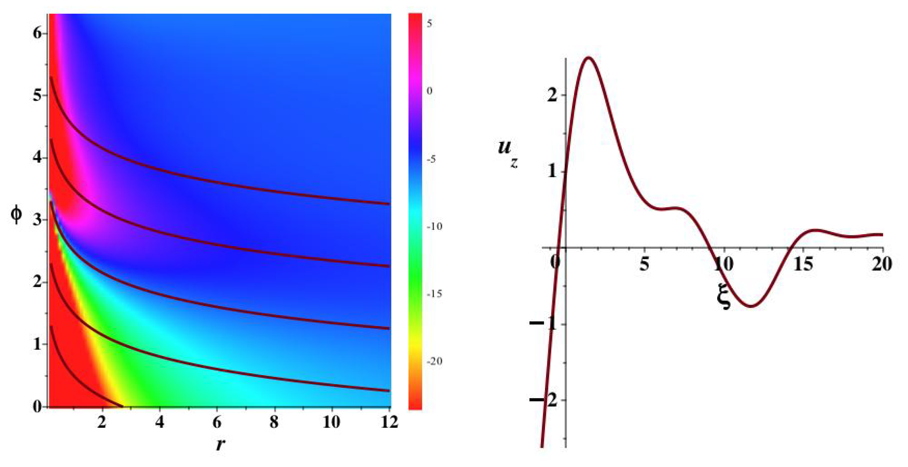
At lower right the same coordinate line is combined with a stream line congruence when the direction of rotation is reversed (), but all other parameters are the same. The stream line integration in that case is over the range and there is a singularity at . In Figure 5 we show that the z velocity is also reversed so that there is reverse thrust with the reverse rotation as expected.
The left image of Figure 5 shows the scaled z velocity corresponding to the scaled velocity shown in Figure 3. The lines are the coordinate lines stepping from to in steps of 2 units. The Navier-Stokes singularity locus would be at . The right image shows the velocity for the reversed propeller (). The thrust is reversed. All of the velocities and pressure can be displayed as in the left image, but that is best left for a more engineering study.
7. Steady, Non Axially Symmetric, Euler Flow
We restrict our study of the zero viscosity flow to the case and and because it allows some comparison with a similar analytic case that includes viscosity in section (Section 4). The parameters and are strictly non zero and .
From continuity, we conclude that is constant, and hence with velocity in units of
Moreover the azimuthal Euler equation integrates immediately to give (H in units of )
where is an arbitrary constant corresponding to external pressure plus potential.
The equation for integrates formally to
where we have set
The last three equations solve the problem once is known. The latter follows from the solution of the radial Euler equation which, after substituting for and H from above, takes the form
Here the constant is also in units of , and . If we set
then the solution for is
This allows all other quantities to be found. The integration constant is .
We note that the tangent solution requires that
which can not happen for . Otherwise the tangent becomes and so that with real
The condition (67) that allows the tangent solution, is also the condition that singularities can exist (except at because ). It will require an external pressure for a singularity to develop. These will appear where () or explicitly on a logarithmic spiral (fixed value of and ) given by
At the singularity appears at (taking )
provided is chosen so that this is less that . With , and , this becomes on taking . In radius at fixed angle, say , the singular spiral with is met at .
The viscous case studied in section (Section 4) had no point singularity. The only difference besides the lack of viscosity is non axial symmetry of this Euler version.
The quantities H and are given directly by equations (61) and (60) respectively. Equation (62) gives for the singular (B real) case
and the becomes when equation (67) is reversed, and B becomes .
According to equation (71) if , then has logarithmic singularities at the singularities of . There are only logarithmic singularities at infinity in the non singular case.
The radial velocity has singularities where does, as does the pressure function.
8. Discussion
The main contribution of this paper is the reduction of the Navier-Stokes equations, using a combination of invariants under a Lie symmetry as the independent variable. This led to scale invariance and ordinary non-linear equations. The flow is described in terms of logarithmic spirals.
We have used this formulation to study a simple axially symmetric flow, related to astrophysical accretion discs.The flow is free of singularities at all scales. A related Euler flow is also discussed where singularities do occur.
We have also presented two approximations to physical problems. One is Hele-Shaw flow and the other allows the properties of equiangular propellers to be calculated. The Hele-Shaw example does not allow a rigorous study with our formulation, but the formulation can be of real help in a complete engineering design of logarithmic spiral propeller blades.
Acknowledgments
Queen’s University has supported this work by allowing privileges available to an Emeritus professor. Dr Judith Irwin has also encouraged this work. Queen’s University at Kingston supported this article by granting me emeritus status. Professor Judith Irwin has provided her usual wise advice.
Appendix A
In this appendix we illustrate the algebra used in reducing the Navier-Stokes equations to the ordinary equations used in the text. We restrict ourselves to deriving the radial equation of motion in the steady state, because the other equations follow similarly.
We begin by gathering from the text the essential relations. These are
We recall the dynamic equations (1)
These are used together with the incompressible condition .
The radial equation follows from the RHS of equation (1). We need the radial component of the curl of and the radial component of . This requires knowing and . The calculation of follows from
which becomes ( and )
We can now compute the radial component of the curl of the vorticity as multiplied by from
Using the relations (A1) at the beginning of the appendix, and the expression for and above we find
The second term on the right of the radial component of equation (1), is an inertial quantity equal to the radial component of the cross product of the velocity and the vorticity in the form
which requires only substitution from the results above to take the form
By subtraction of these two terms on the right hand side (RHS) of equation (1), and subsequent equality to the left hand side (LHS) computed below, we can obtain the radial equation.
On the LHS
which becomes
Finally, we equate the terms left and right, introduce , and rearrange slightly, to obtain equation (20).
| 1 | Here the co-vector is resolved along space-time units so for the length co-vector, there is one unit of space and zero units of time |
References
- Meneveau, C.; Katz, J. Scale-Invariance and Turbulence Models for Large-Eddy Simulation. Annual Review of Fluid Mechanics 2000, 32, 1–32. [Google Scholar] [CrossRef]
- Schaefer-Rolffs, U. The Scale Invariance Criterion for Geophysical Fluids. European Journal of Mechanics-B fluids 2019, 74, 92–98. [Google Scholar] [CrossRef]
- Carter, B.; Henriksen, R.N. A systematic approach to self-similarity in Newtonian space-time. Journal of Mathematical Physics 1991, 32, 2580–2597. [Google Scholar] [CrossRef]
- Henriksen, R. Scale Invariance; Wiley-VCH, 2015.
- Wang, K.; Sprinkle, B.; Zuo, M.; Ristroph, L. Centrifugal Flows Drive Reverse Rotation of Feynman’s Sprinkler. Phys. Rev. Lett. 2024, 132, 044003. [Google Scholar] [CrossRef] [PubMed]
- Bogoyavlenskij, O. The new effect of oscillations of the total angular momentum vector of a viscous fluid. Physics of Fluids 2022, 34, 1–10. [Google Scholar] [CrossRef]
- Lynden-Bell, D.; Pringle, J.E. The evolution of viscous discs and the origin of the nebular variables. mnras 1974, 168, 603–637. [Google Scholar] [CrossRef]
- Abramowitz, M.; Stegun, I.A. Handbook of mathematical functions : with formulas, graphs, and mathematical tables; 1970.
- Gowen, S.D.; Videbæk, T.E.; Nagel, S.R. Measurement of pressure gradients near the interface in the viscous fingering instability. Physical Review Fluids 2024, arXiv:physics.flu-dyn/2402.01924]9, 053902. [Google Scholar] [CrossRef]
Figure 1.
The figure shows the two point () flow velocities (to be multiplied by , and one instantaneous ’stream line’ cluster for the case when , and the eigenvalue is . The boundary conditions were , at the end points, plus . The radial velocity is at upper left, the pressure function at upper right, the azimuthal velocity at lower left and a ’stream line’ cluster is shown at lower right. The stream line cluster shown passes through and as a tube f radius centred on the plane .
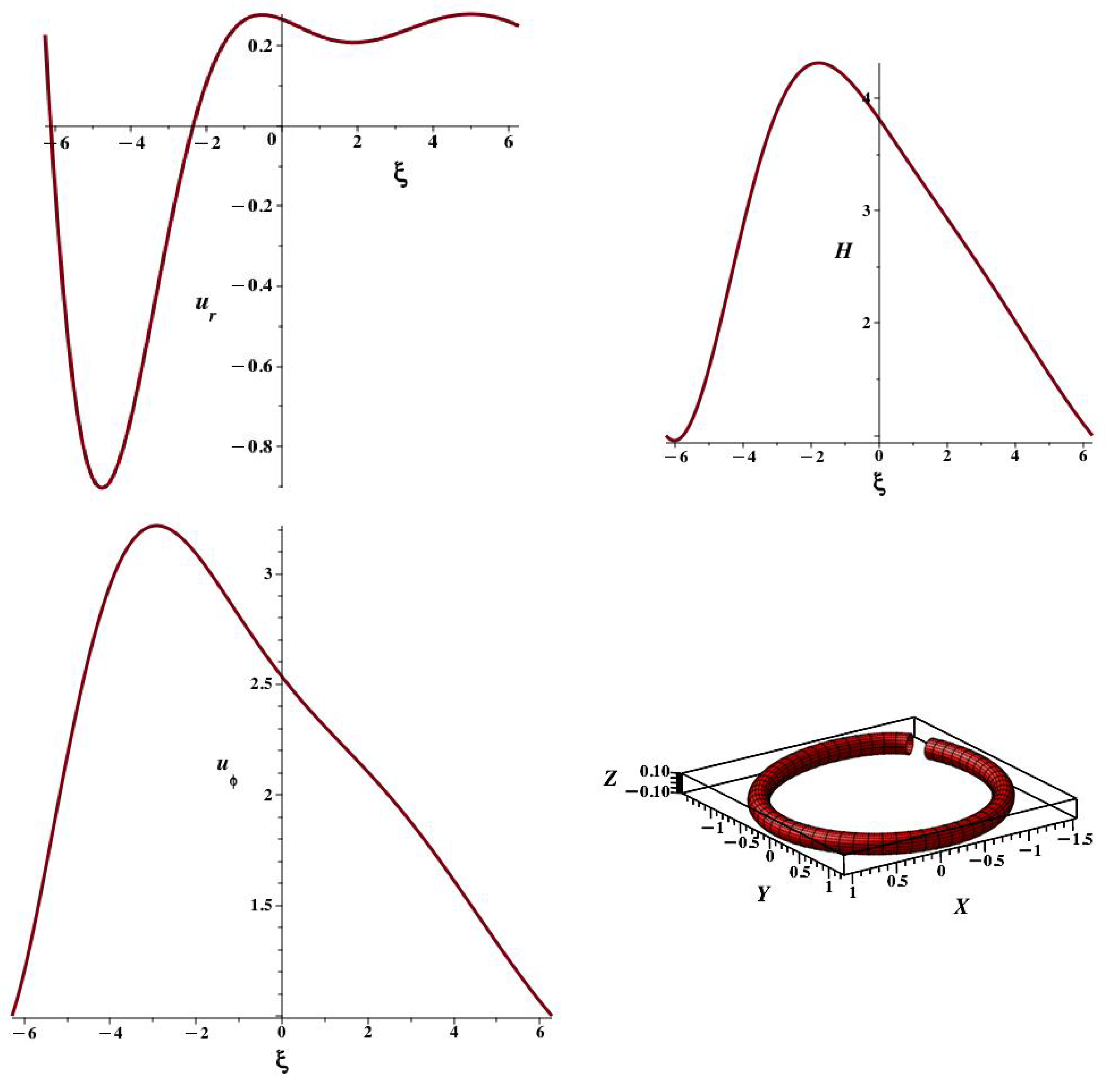
Figure 2.
The figure shows the flow velocities as a function of and one instantaneous stream line () for the case when , and is . The initial conditions were , , and . The radial velocity is at upper left, the pressure function at upper right, the azimuthal velocity at lower left and one ‘stream line’ is shown at lower right. For reference lines of constant are shown in the range in steps of 1. They converge on at different angles.
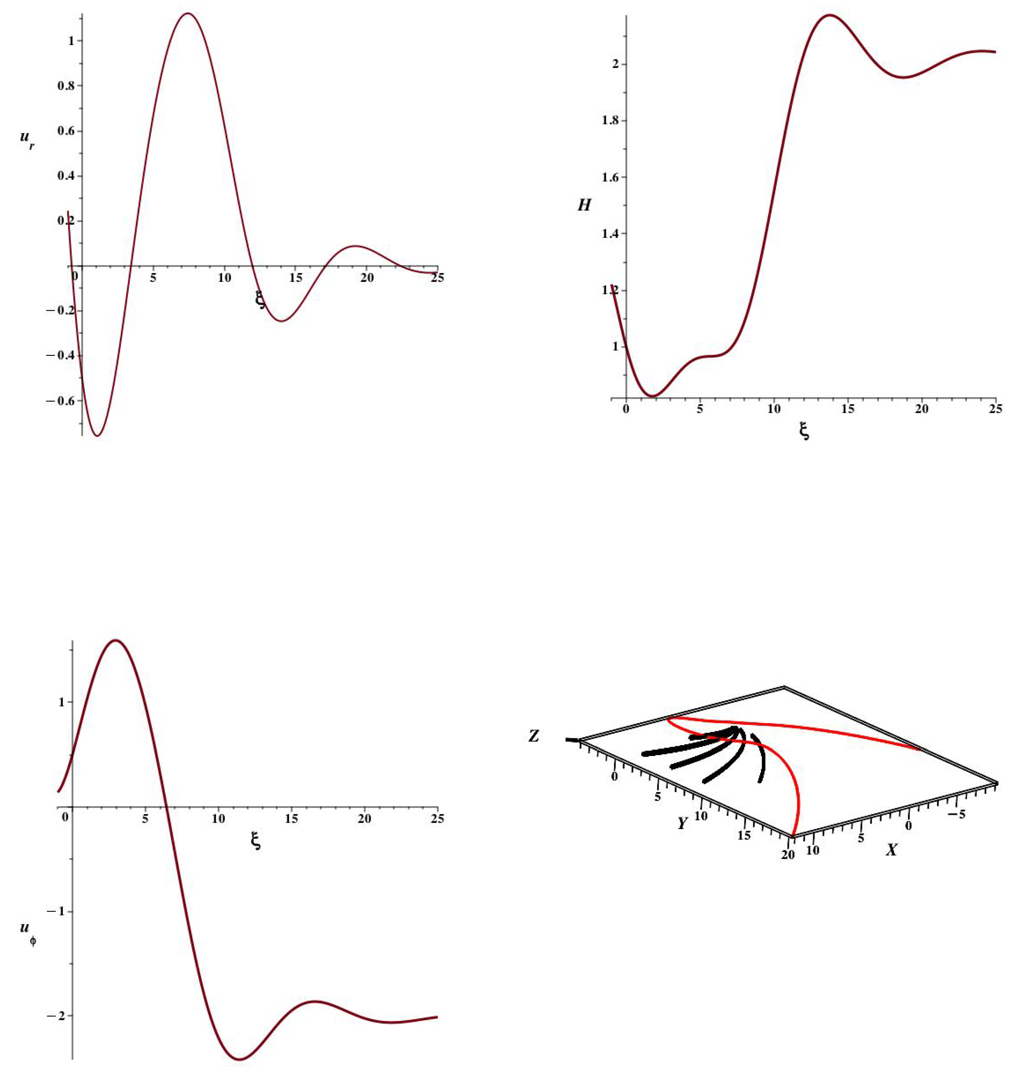
Figure 3.
The figure shows the flow velocities and the pressure variation for our standard example with , and . The initial conditions are and . The constant . There is a singularity in the fluid equations at . At upper left we show , at upper right and at lower left. The pressure is at lower right.
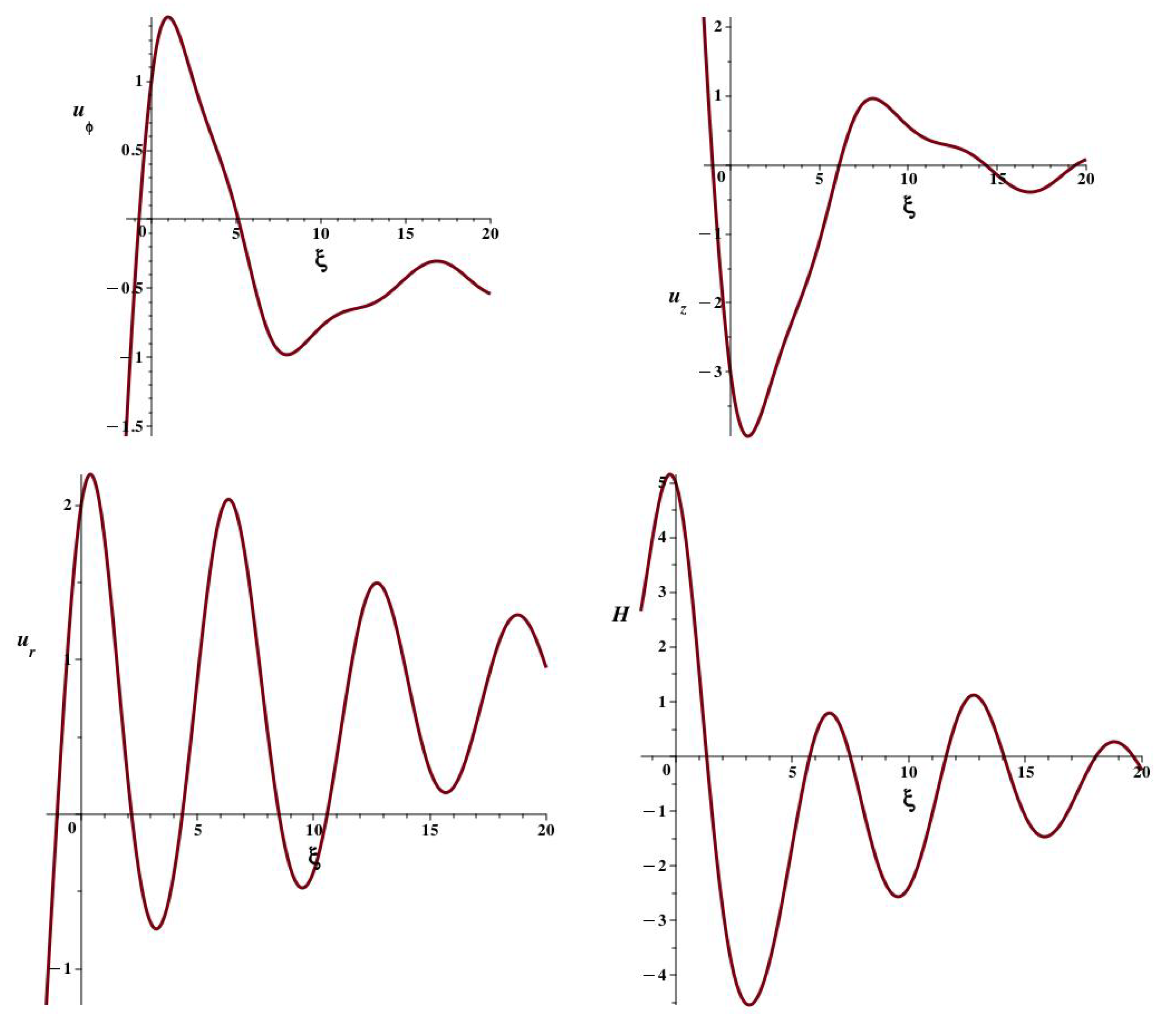
Figure 4.
The congruence of stream line shown at upper left passes near or through and and . It is integrated over . At upper right we show the coordinate line line for , which also passes through , and . At lower left the two are combined as a kind of one bladed logaritmic spiral propeller. At lower right the same coordinate line is combined with a congruence of stream lines calculated for over the arc length .
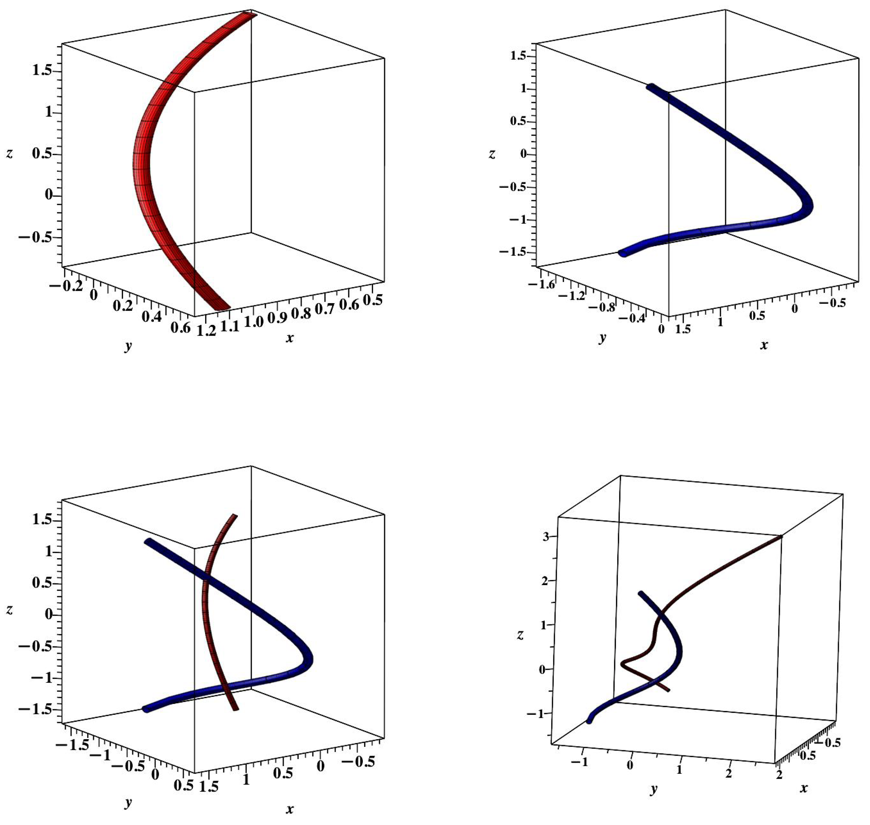
Figure 5.
The right hand image shows the velocity for the reversed propeller with . The flow near is now positive, giving reverse thrust. On the left we show for the standard case () projected onto the plane. There is strong negative velocity at small angle and radius. The coordinate lines projected onto the plane are shown for (the smaller line) until in steps of 2.
Disclaimer/Publisher’s Note: The statements, opinions and data contained in all publications are solely those of the individual author(s) and contributor(s) and not of MDPI and/or the editor(s). MDPI and/or the editor(s) disclaim responsibility for any injury to people or property resulting from any ideas, methods, instructions or products referred to in the content. |
© 2025 by the authors. Licensee MDPI, Basel, Switzerland. This article is an open access article distributed under the terms and conditions of the Creative Commons Attribution (CC BY) license (http://creativecommons.org/licenses/by/4.0/).
Copyright: This open access article is published under a Creative Commons CC BY 4.0 license, which permit the free download, distribution, and reuse, provided that the author and preprint are cited in any reuse.


