
Submitted:
25 February 2025
Posted:
27 February 2025
You are already at the latest version
Abstract
Generalized closeness is a recently defined centrality measure. Decay stability, based on generalized closeness, was studied in [Coroničova Hurajova et al. Math. Scand., 2018, 123: 39-50] and several conjectures on decay stability of certain graph classes were put forward. Here we disprove two conjectures by showing that the Cartesian and strong products of paths are not decay stable.
Keywords:
graph products
; centrality measure
; decay stability
1. Introduction
Centrality has been an interesting notion in graph theory since its beginnings. A significant spike of interest in centrality occurred in the late 1940s and early 1950s in the social sciences [8]. A more interdisciplinary approach emerged in the late 1990s and the early 2000s in the nomenclature of Network Science [17]. Since the 2000s, centrality metrics have grown in significance in communication networks, in particular in regard to efficient information transmission, fault tolerance, and vulnerability against attacks. See a recent comprehensive survey [16].
In [9], closeness (or closeness centrality) of a connected graph was defined as a measure of centrality of a node in a network as
where is the distance between vertices and . Thus, the more central a node is, the closer it is to all other nodes. For example, in an information network, closeness is a useful measure that estimates how fast the flow of information would be through a given node to other nodes. In the social network analysis, closeness can be used for finding the individuals who are best placed to influence the entire network most quickly.
Dangalchev [3] proposes a rather different definition, which can also be used effectively for disconnected graphs and allows to create convenient formulae for graph operations. In [3], point closeness of vertex is defined by
with The graph closeness is then defined as
Dangalchev emphasizes that, in contrast to (1), the graph closeness based on (2) can be used also for disconnected graphs, because if then As mentioned in [14], there are many graph theoretical parameters depending upon the distance such as vertex and edge betweenness, average vertex and edge betweenness, normalized average vertex and edge betweenness, closeness, vertex residual closeness. The aim of closeness and residual closeness is to measure the vulnerability even when the actions disconnect the graph. It was explained in [1,3] that residual closeness is considered to be more sensitive vulnerability measure than some other known measures. Closeness of some graph classes has been studied in [3,5,10]. Several interesting results on closeness of graph transformations, regarding vertex residual closeness, normalized vertex residual closeness and closeness centrality for some classes of graphs have been obtained in [14,15].
The base in the definition of closeness (2) can be replaced with any constant giving rise to a definition generalized closeness as
Closeness centrality seems to be a very natural concept, as it has been reinvented and studied independently under different names several times.
For example, Tsakas [13] studies decay centrality, the notion equivalent to generalized closeness (3). He shows close connection between decay centrality and two well-studied and computationally cheaper measures, namely the degree and closeness centrality. Among other things he observes that for sufficiently low values of the nodes that maximize (3) are those of maximal degree, and on the other side, for sufficiently large the nodes that maximize closeness also maximize decay centrality (3).
We wish to note that the definition of generalized closeness was given also in [4] where the author initiates the study of generalized closeness and, among other observations, argues that choosing the proper base for the closeness depends on the properties of the network we want to investigate. Therefore, considering closeness for an arbitrary base can give some very interesting issues for research. We wish to note that also, as observed in [11] we clearly have , where H is the Hosoya -Wiener polynomial [7,12], a well-known notion in mathematical chemistry.
The rest of this paper is organized as follows. In Section 2 we discuss generalized closeness in relation to distance degree sequences and define a new relation on the set of nodes. Using this relation we derive a criterion for decay-stable graphs (Theorem 1 and Theorem 2). In Section 3 we study decay-stability of two graph structures, Cartesian products of paths and strong products of paths. Two conjectures of [2] are disproved by providing counterexamples. In the last section, ideas for future work are given. In particular, we briefly comment another conjecture of [2], that is likely correct.
2. Decay-stability
Let . The centrality index defines the ranking of G in the following way [2]: If is a permutation of such that
is a non-increasing sequence, then -ranking of G is
Distinct overlined blocks contain distinct values of index (in decreasing order), the values within a block are the same. Of course, this ranking of index depends on .
Generalized closeness of a vertex v is a polynomial of degree (eccentricity), its coefficients are equal to terms of the distance degree sequence , the sequence where is the number of vertices of the distance i from vertex v. Obviously, , and
Taking polynomials for all , their roots in are called decay thresholds of G. Graphs where ranking does not change for different values of are called decay-stable graphs. Otherwise, we will call the graph decay-unstable. In the following, we will be interested in graphs that are decay-stable.
Proposition 1.
Let and , . If for each j, it holds
then for any
If there exists j such that , then .
Proof.
Also note that, for any , implies that
and the equality holds exactly when for all i. Hence
as needed. Finally, if for some j, then in case the sum above is strictly positive. Hence .
In the remaining case, , we have
using the inequality (5). This completes the proof. □
In Proposition 1 we recalled the result of Proposition 2.2. from [2], but we wish to note, however, that the last part of the proof in [2] is false although the claim is correct. For example, in the graph from Figure 1 we have and . Although , and , the distance degree sequences for vertices 2 and 3 have the same length, . The authors in [2] erroneously claimed that in this case !
We now define a new relation on the set of vertices :
Definition 1.
Let and . Then if and only if the inequality (4) holds for all .
It is obvious that this relation is reflexive, antisymmetric and transitive, so it defines a partial order on a set .
Theorem 1.
A graph G is decay-stable if and only if the relation ⪰ defines a linear (total) order on the set , i.e. for each or holds.
Proof.
First assume that graph G is decay-stable. Then for all and for all . Thus, either for all , or for all . That means or .
Conversely, let ⪰ define a linear order on . Then for each or . Let . Then inequality (4) holds for each , where . By Proposition 1 then for all , It follows that G is decay-stable. □
Immediate corollary to the last theorem is the following, observed already in [2],
Corollary 1.
Any distance degree regular graph is decay-stable.
The next corollary is more general. As we find the statement quite important, we state it as a theorem.
Theorem 2.
Let . If for two vertices we have
then G is decay-unstable.
Proof.
Let and , and , . From we have , and hence
On the other hand, as ,
Therefore, neither nor , and, by Theorem 1, G is not decay-stable. □
3. Decay Stability of Products of Paths
We now discuss two conjectures of [2] on decay stability of certain graphs, namely Cartesian and Strong products of paths. It was proven that
Theorem 3.
[2] If graph G is decay-stable, then, for any positive integer n, the Cartesian product is also decay-stable.
Corollary 2.
[2] All graphs of diameter 2 are decay-stable, all regular graphs of diameter 3 are decay-stable.
In [2], also the following two conjectures were given
Conjecture 1.
[2] For all positive integers , the l-dimensional grid is decay-stable.
Conjecture 2.
[2] The strong product is decay-stable for all positive integers k and l.
Here we provide conunterexamples to both conjectures.
The Cartesian product of two graphs is defined as a graph with vertex set where two vertices and are adjacent precisely if and , or and . Recall that the l-dimensional grid is Cartesian product of paths .
For a path and its vertices and , it is obvious
a sequence of length , where number 2 occurs exactly -times (never in case ). Thus
It is obvious that the path is decay-stable since from Definition 1 and Theorem 1 it follows that for its vertices we have a linear order
The next examples prove that Conjecture 1 is wrong.
Example 1.
Take a grid and its vertices and . Then
Observe that , but . Thus neither nor . Hence, the Cartesian product of two paths is decay-unstable.
Example 2.
Take a grid and its vertices and . Then
and, obviously, the Cartesian product is decay-unstable.
On the positive side, we can show that is decay stable for any It is obvious that for the vertices on the corners: , or
s sequence of length k, where number 2 occurs exactly -times. For the vertices we have
where number 2 occurs exactly -times. For a typical vertex inside the grid, given by or the distance degree sequence is:
Here, the number 4 appears exactly - times. The number 3 appears at position j either once or not at all, in the special case where k is odd and . The same condition applies to the number 1, which appears at the end of the sequence. The number 2 appears exactly -times. Thus, for odd k we have a linear order
Similarly, for even k, we have
It is not hard to see that Cartesian products and are decay stable. Summarizing the observations and the examples above, we can write the following proposition.
Proposition 2.
The Cartesian product of two paths , , is decay-unstable.
In the strong product of graphs, , two distinct vertices and are adjacent if and only if: and v is adjacent to , or and u is adjacent to , or u is adjacent to and v is adjacent to .
Similarly to above discussion about Cartesian products, we can prove the following statement.
Proposition 3.
The strong product of two paths , , is decay-unstable.
It is obvious that the strong products , and are decay stable.
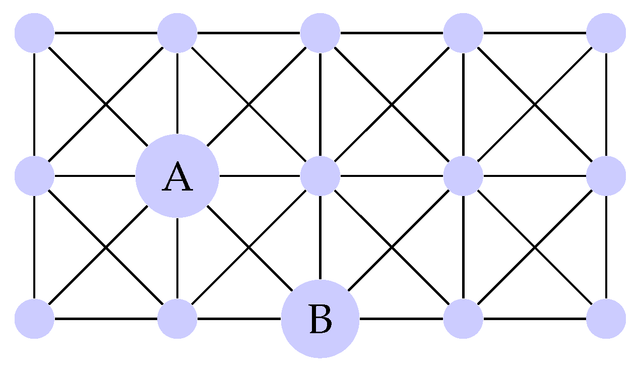
Example 3.
Take a strong product of . Then (see see Figure 2),
Thus neither nor .
4. Conclusions and Future Work
In this paper we have shown that two conjectures stated in [2] do not hold by providing several examples. On the positive side, we prove that the conjeture holds for an infinite set of Cartesian products. Thus it may be interesting research task to characterize the subsets of decay stable Cartesian and strong products of paths.
The authors of our main reference also put forward another conjecture
Conjecture 3.
[2] Almost all tress are not decay-stable.
which, in our opinion is likely to be true. We only briefly explain the main ideas here. A formal proof with all details however seems not to be simple, and we leave it as a challenge for future work.
In short, the main idea of a possible proof of conjecture for random recursive trees (RRT) is a follows. Theorem 2 implies that on decay stable trees, the degrees of vertices must form a nonicreasing sequence from the center (centers) to the leaves. As this is a strong condition that likely does not hold for majority of trees, by itself it gives some evidence that the Conjecture 3 is true. A formal proof that almost all trees are not decay-stable is however perhaps not trivial. In particular, because in details it depends on the model of random trees chosen.
Recall that Eslava [6] proves that in RRT, the distributions of depths of vertices attaining the maximum degree are asymptotically normal and independent. Furthermore, the number of such vertices converges to a mixture of Poisson random variables conditioned to be strictly positive. Here, the depth is the distance from the root, that is any vertex from which the generation of tree starts. So in case when the root is at the same time the center, the observation implies that with high probability there exists a vertex of large degree that is not a center, hence the conjecture may follow.
Funding
The research was partially funded by the Slovenian Research and Innovation Agency (ARIS) through project P2-0248 and through the annual work program of Rudolfovo.
Conflicts of Interest
The authors declare no conflicts of interest.
References
- Aytaç A, Odabaş Z N. Residual Closeness of Wheels and Related Networks. Int. J. Found. Comput. S. 2011, 22(05), 1229–1240.
- Coroničova Hurajova J., Gago S. and Madaras T., On decay centrality in graphs, Math. Scand., 2018. 123: 39-50.
- Dangalchev, C. Residual closeness in networks. Physica A 2006, 365, 556–564. [Google Scholar] [CrossRef]
- Dangalchev, C. Residual Closeness and Generalized Closeness. Int. J. Found. Comput. S. 2011, 22(08), 1939–1948. [Google Scholar]
- Dangalchev, C. Residual Closeness of Generalized Thorn Graphs. Fundam. Inform. 2018, 162, 1–15. [Google Scholar]
- Eslava L, Depth of vertices with high degree in random recursive trees, ALEA. Lat. Am. J. Probab. Math. Stat. 2022, 19, 839–857. [CrossRef]
- Hosoya, H. Onsomecountingpolynomialsinchemistry. DiscreteAppliedMathematics 1988, 19(1–3), 239–257. [Google Scholar] [CrossRef]
- Katz, L. A new status index derived from sociometric analysis. Psychometrika 18, 39–43 (1953). [CrossRef]
- Latora V, Marchiori M. Efficient behavior of small-world networks. Phys. Rev. Lett. 2001, 87(19), 198701-(1–4). [CrossRef]
- Odabaş Z N, Aytaç A. Residual Closeness in Cycles and Related Networks. Fundam. Inform. 2013, 124(3), 297–307.
- Rupnik Poklukar D, Žerovnik J., Reliability Hosoya-Wiener Polynomial of Double Weighted Trees. Fundam. Inform. 2016, 147(4), 447–456. [CrossRef]
- Sagan B E, Yeh Y-N, Zhang P, The Wiener polynomial of a graph, Int. J. Quantum Chem. 1996, 60, 959–969. [CrossRef]
- Tsakas N, On decay centrality, (January 4, 2017).Available at: https://ssrn.com/abstract=2767012 or http://dx.doi.org/10.2139/ssrn.2767012.
- Turacı T, Ökten M. Vulnerability of Mycielski Graphs via Residual Closeness. Ars Combinatoria 2015, 118, 419–427.
- Turacı T, Aytaç V. Residual Closeness Of Splitting Networks. Ars Combinatoria 2017, 130, 17–27.
- Wan Z, Mahajan Y, Kang B W, Moore T J, Cho J H. A Survey on Centrality Metrics and Their Network Resilience Analysis, IEEE Access, vol.9, pp. 104773-104819, 2021. [CrossRef]
- NRC, Network Science. Washington, DC, USA: The National Academies Press, 2005. [Online]. Available: https://www.nap.edu/catalog/11516/network-science.
Figure 1.
An example of a tree with vertices
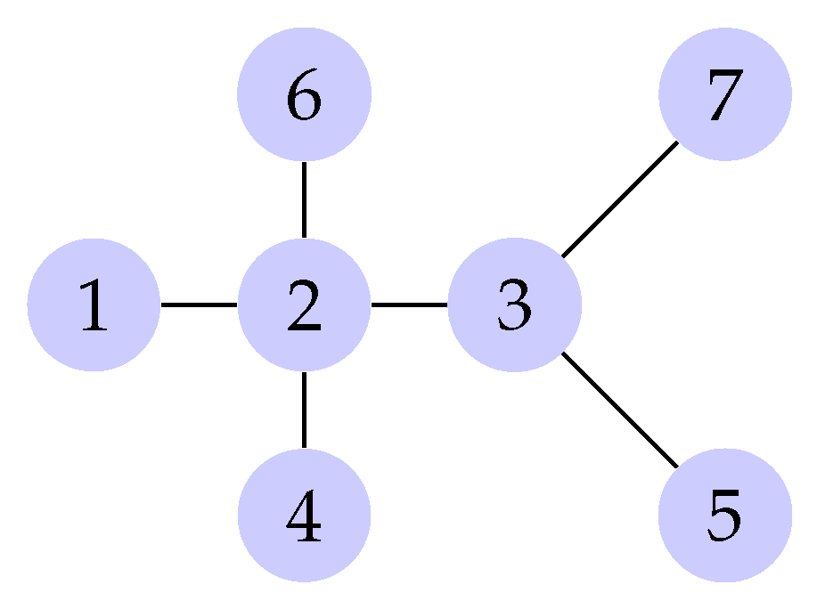
Figure 2.
Graph .
Disclaimer/Publisher’s Note: The statements, opinions and data contained in all publications are solely those of the individual author(s) and contributor(s) and not of MDPI and/or the editor(s). MDPI and/or the editor(s) disclaim responsibility for any injury to people or property resulting from any ideas, methods, instructions or products referred to in the content. |
© 2025 by the authors. Licensee MDPI, Basel, Switzerland. This article is an open access article distributed under the terms and conditions of the Creative Commons Attribution (CC BY) license (http://creativecommons.org/licenses/by/4.0/).
Copyright: This open access article is published under a Creative Commons CC BY 4.0 license, which permit the free download, distribution, and reuse, provided that the author and preprint are cited in any reuse.


