Auto-stabilized Electron 2.0

1. Introduction

The paradox of electron stability has been recognized since its discovery[1,2,3,4]. Instability is inevitable in any system with charge distributed over an extended volume. There have been several conjectures to explain stability (i) a shell of non-electromagnetic origin to contain the field (Poincare’ stress), (ii) using radiation reaction to compensate the outward pressure (Abraham-Lorentz equation), (iii) dimensional regularization etc. For details see [9].

The approaches referred to have one common motivation: that infinities are a mathematical anomaly; instead they are intrinsic to the theory.

We claim instead that the appearance of infinities is the consequence of ignoring basic physical phenomena. The infinities are real. In the sections below we describe what these are and calculate the resulting corrected electron radius and mass from first principles.

1.1. Computation Algorithm

Using standard quantum electrodynamics to calculate the mass shift for a free electron, Feynman’s final result is

$$\Delta m={\displaystyle \frac{4\pi e^2}{2mi}}{\int }_{-\infty }^{\infty }{\displaystyle \frac{\tilde{u}\left(2m+2k\right)u}{k^2-2\overrightarrow{p}·\overrightarrow{k}}}{\displaystyle \frac{d^{4}k}{{\left(2\pi \right)}^4}}{\displaystyle \frac{1}{k^2}}$$

(1)

for the mass correction $\Delta m$ [5] where m is the experimental mass and e the charge of the electron; the variables are k and p, the four-momenta of photons and p the electron.

The integral being of the form $d^{4}k/k^4$ is intrinsically divergent. Feynman obviates the divergence by modifying the photon kernel. The effect is to alter the laws of electrodynamics at short distances. Although no reason exists to justify this alteration, since there is no evidence that the laws of electrodynamics are inadequate at short distances. Even so with this alteration the integral is logarithmically divergent; it also necessitates the introduction of a free parameter. The puzzle remains unsolved.

The diagram Figure 1 represents the electron emitting and absorbing a single photon.

1.2. Near Field

A way out of this dilemma is to re-interpret the one-loop correction and relate it to fields in the vicinity of a classical radiation source. Surrounding any source radiating at a wavelength $\lambda$ there is a near zone which extends to $r=\lambda /2\pi .$ In terms of the wave-vector $\kappa$ the condition that makes this so is $\kappa ·r=1$ . The near zone is what is called the velocity field in the Liĕnard-Wiechert potentials.

The radius of the near zone scales inversely as the wave-vector. The larger the wave vector the smaller the near zone. Within the near zone the fields are Coulomb-like. The fields exert a radially outward pressure. Outside the near zone retardation sets in; fields acquire a transverse component; they propagate. An excellent animation of the interaction between accelerating charge and fields be found in [7].

Field energy is stored within the near zone. This energy manifests itself as an excess mass in Eq. (1.1). With an accelerating charge, energy is continuously exchanged between fields and source in the near zone; pictorially represented as the emission and absorption of single photons Figure 1. One consequence is the radiation reaction on the charge. Higher order diagrams correspond to quadrupole, octupole and higher order fields. Identifying this mechanism is the central concept of this paper.

1.3. Gravitation

We can see how gravity comes into the picture. For the electron radius we can choose two options. One from special relativity - classical radius, the other from quantum mechanics - Compton wavelength. The energy density of an electron of radius r equal to a Compton wavelength ( ${\lambda }_C$ ) can be estimated. Setting $r={\lambda }_C$

$${\displaystyle \frac{e^2}{4\pi {ϵ}_{0}r}}{\displaystyle \frac{1}{\left(4\pi /3\right)r^3}}={\displaystyle \frac{e^2}{4\pi {ϵ}_0}}{\displaystyle \frac{3}{4\pi }}{\displaystyle \frac{1}{{\left({\lambda }_C\right)}^4}}={\displaystyle \frac{e^2}{4\pi {ϵ}_0}}{\displaystyle \frac{3}{4\pi }}{\left({\displaystyle \genfrac{}{}{0pt}{}{mc}{h}}\right)}^4={10}^{18}J/m^3$$

(2)

which is $\approx {10}^{13}$ atmospheres; by comparison the pressure at the center of the Sun is ${10}^{11}$ atmospheres. This shows that such high energy densities are not just the purview of astrophysical sources but are common among elementary particles.

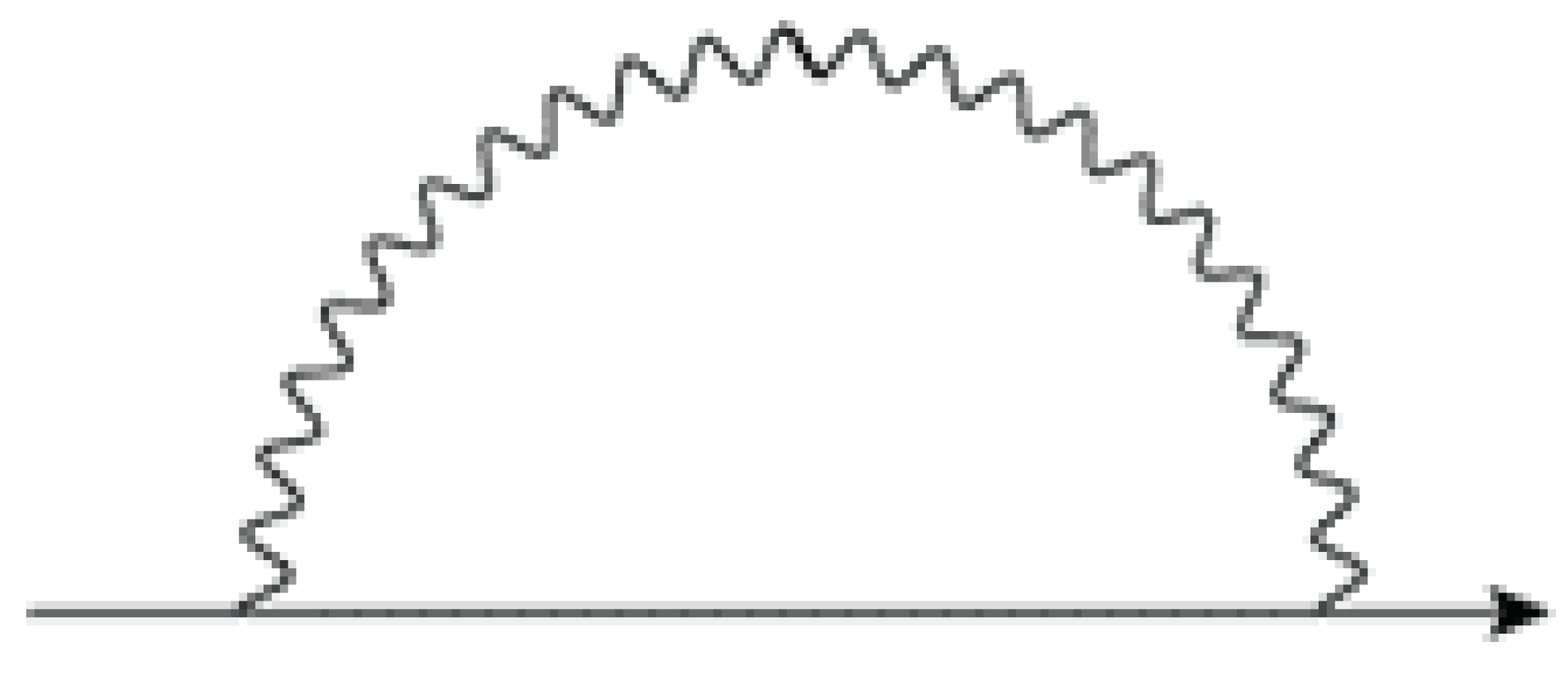
Clearly under these conditions energy densities are high enough to alter the metric in the vicinity of the electron. At these densities virtual excitations generate a curved metric. Virtual excitations loop back to the source along geodesics of the distorted metric. For example in Figure 1 the emission and absorption of virtual photons occurs in a curved metric. General relativistic effects not only cannot be ignored; they become essential part of the dynamics of the electron. Gravitation is part of the electron.

It is evident that theories that rely on flat space geometry are inadequate; the engendered divergences are evidence that in such theories a major reservoir of energy, the curved metric, is being ignored. The enormous outward forces cannot be balanced in flat space; curved space-time must be included.

There have been attempts to include gravity in QED phenomena. An early example is Isham, Salam and Strathdee, [8] and others.

1.4. Gravitating Electron

In this paper we incorporate gravitation first by integrating Eq. (1.1) up to an upper limit for k . The upper limit is an unknown for now. We set the momentum

$$k=\hslash \kappa =\hslash {\displaystyle \frac{2\pi }{\lambda }}$$

(3)

where $\kappa$ is the wave number. The corresponding near zone radius for $\lambda$ is $r=\lambda /2\pi .$

Integrating Eq. (1.1) we get for the mass correction (see Appendix)

$$\Delta m\equiv \mu \left(\eta \right)={\displaystyle \frac{\alpha m}{2\pi }}\left[-{\displaystyle \frac{\eta }{2}}\sqrt{1+{\displaystyle \frac{1}{\eta }}}+\eta +ln\left\{\sqrt{\eta }\left(\eta \sqrt{1+{\displaystyle \frac{1}{\eta }}}+1\right)\right\}\right]$$

(4)

in terms of a dimensionless variable

$$\eta \equiv h/2mcr={\lambda }_C/4\pi r$$

(5)

We have redefined $\Delta m\equiv \mu \left(\eta \right)$.

The energy density, or equivalently the stress tensor, alters the metric within the near zone. The net result is an inward pressure. Thus there are two competing pressures - an outward pressure from the field and an inward pressure from the metric. It is this balancing mechanism that stabilizes the electron.

Analogous to the Sun where the radiation pressure (or Fermi pressure in the case of white dwarfs or neutron stars) is balanced by the inward gravitational pressure.

As the upper limit of the $k-$ vector in Eq. (1.1) is increased, the stress tensor also increases, as well as the inward gravitation induced pressure. The electron is auto-stabilized.

Equating the two competing pressures yields an upper limit for $k.$ We will calculate this limit.

In order to get an explicit condition for equilibrium we use the Einstein equation. We start with a line element of the form

$$d{s}^2=e^{2\mathsf{\Phi }}{c}^{2}d{t}^2-e^{2\mathsf{\Lambda }}d{r}^2-r^2\left(d{\theta }^2+{sin}^2\theta d{\varphi }^2\right)$$

(6)

Fields within the near zone are treated as a perfect fluid. The elements of the stress tensor are

$$T^{\widehat{0}\widehat{0}}=\rho ;T^{\widehat{1}\widehat{1}}=T^{\widehat{2}\widehat{2}}=T^{\widehat{3}\widehat{3}}=P$$

(7)

in the fluid’s orthonormal rest-frame basis vectors. Imposing momentum conservation and spherical symmetry the relevant Einstein equations are

$$G^{\widehat{0}\widehat{0}}={\displaystyle \frac{e^{2\mathsf{\Phi }-2\mathsf{\Lambda }}\left(-1+e^{\mathsf{\Lambda }}+2r{\mathsf{\Lambda }}^2\right)}{r^2}}=8\pi T^{\widehat{0}\widehat{0}}=8\pi \rho$$

(8)

$$G^{\widehat{1}\widehat{1}}={\displaystyle \frac{1-2e^{2\mathsf{\Lambda }}+2rd\mathsf{\Phi }/dr}{r^2}}=8\pi T^{\widehat{1}\widehat{1}}=8\pi P$$

(9)

We define a new metric coefficient $\mu \left(r\right)$ (same as in Eq. (4) as

$$g_{11}=e^{2\mathsf{\Lambda }}\equiv {\displaystyle \frac{1}{1-\frac{2\mu \left(r\right)}{r}}}$$

(10)

$\mu \left(r\right)$ is the corrected mass inside the radius r. The time-time component of Eq. (8) [6] takes the form

$${\displaystyle \frac{d\mu }{dr}}=4\pi r^2\rho$$

(11)

whereas radial-radial component of Eq. (9 ) [6] takes the form

$${\displaystyle \frac{d\mathsf{\Phi }}{dr}}=2{\displaystyle \frac{\mu +4\pi r^{3}P}{r\left(r-2\mu \right)}}$$

(12)

The proper density is

$$\rho ={\displaystyle \frac{1}{4\pi r^2}}{\displaystyle \frac{1}{\sqrt{g_{11}}}}{\displaystyle \frac{d\mu }{dr}}$$

(13)

Since the volume element

$$dV=\sqrt{|g_{11}|}{r}^{2}sin\theta d\theta d\varphi dr$$

(14)

In terms of the dimensionless parameter $\eta$ the density derivative is

$${\displaystyle \frac{d\rho }{d\eta }}={\displaystyle \frac{d\rho }{dr}}{\displaystyle \frac{dr}{d\eta }}$$

(15)

These equations when combined with the condition for hydrostatic equilibrium lead to the Tolman-Oppenheimer-Volkov equation

$${\displaystyle \frac{dP\left(r\right)}{dr}}=-\left(\rho \left(r\right)+P\left(r\right)\right){\displaystyle \frac{\left(\mu \left(r\right)+4\pi r^{3}P\left(r\right)\right)}{r^2\left(1-\frac{2\mu \left(r\right)}{r}\right)}}$$

(16)

This first order differential equation can be solved once the relation between pressure $P\left(r\right)$ and density $\rho \left(r\right)$ is established. The negative slope guarantees the decrease of $P\left(r\right)$ until for some value of r , $P\left(r\right)=0$ . We seek this value of r. The free parameter is adjusted to ensure that m(r) goes to zero as r goes to zero.

1.5. Equation of State

We can derive an equation of state - relate $P\left(r\right)$ with $\rho \left(r\right).$ We use the work equation

$$dE=-PdV;{\displaystyle \frac{dE}{dV}}=-P$$

(17)

Also $E=\rho V$

$$\begin{array}{ccc}\hfill dE& =& Vd\rho +\rho dV\hfill \end{array}$$

(18)

$$\begin{array}{ccc}\hfill {\displaystyle \frac{dE}{dV}}& =& {\displaystyle \frac{d\rho }{dV}}V+\rho =-P\hfill \end{array}$$

(19)

$$\begin{array}{ccc}\hfill {\displaystyle \frac{d\rho }{dV}}& =& {\displaystyle \frac{d\rho }{dr}}{\displaystyle \frac{dr}{dV}}={\displaystyle \frac{d\rho }{dr}}{\left({\displaystyle \genfrac{}{}{0pt}{}{3}{4\pi }}\right)}^{1/3}{V}^{-2/3}\hfill \end{array}$$

(20)

$$\begin{array}{ccc}\hfill {\displaystyle \frac{dE}{dV}}& =& {\displaystyle \frac{d\rho }{dr}}{\left({\displaystyle \genfrac{}{}{0pt}{}{3}{4\pi }}\right)}^{1/3}{V}^{-2/3}V+\rho =-P\hfill \end{array}$$

(21)

The near zone fields have an equation of state which is

$$P=-\rho -{\displaystyle \frac{1}{3}}r{\displaystyle \frac{d\rho }{dr}}$$

(22)

Or in terms of $\mu \left(r\right)$ the equation of state can be written as

$$P=-{\displaystyle \frac{1}{4\pi r^2}}{\displaystyle \frac{1}{\sqrt{g_{11}}}}{\displaystyle \frac{d\mu }{dr}}-{\displaystyle \frac{1}{3}}{\displaystyle \frac{1}{4\pi r}}{\displaystyle \frac{1}{\sqrt{g_{11}}}}{\displaystyle \frac{d^2\mu }{d{r}^2}}$$

(23)

Eq. (16) can be re-written in terms of the variable $\eta .$

$${\displaystyle \frac{dP}{d\eta }}={\displaystyle \frac{dP}{dr}}{\displaystyle \frac{dr}{d\eta }}$$

(24)

We calculate $P\left(\eta \right)$ by integrating ${\displaystyle \frac{dP\left(\eta \right)}{d\eta }}$

$$P\left(\eta \right)=\int {\displaystyle \frac{dP\left(\eta \right)}{d\eta }}d\eta$$

(25)

and find the root of the integral ${\eta }_e$ for which $P\left({\eta }_e\right)=0$; this is the value of $\eta$ and thus the lower limit r or the upper limit k we are looking for.

1.6. Results

In order to simplify the computation we will use an approximation where $\eta \gg 1$ to find the root of Eq. (16).

This allows us to simplify the terms $\mu \left(\eta \right)$ , $\rho \left(\eta \right)$ and $P\left(\eta \right)$ (which has ${\displaystyle \frac{\partial \rho }{\partial \eta }}$ ).

For example for $\eta \gg 1$ , $\rho \left(\eta \right)\to {\displaystyle \frac{{\eta }^4}{2}},{\displaystyle \frac{\partial \rho }{\partial \eta }}\to 2{\eta }^3,$$\mu \left(\eta \right)\to {\displaystyle \frac{\eta }{2}}$. For the root ${\eta }_e$ we get

$${\eta }_e=1.00255876\times {\left({\displaystyle \frac{c^2}{2mG}}{\displaystyle \frac{2\pi }{\alpha }}{\displaystyle \frac{\hslash }{2mc}}\right)}^{1/2}=1.00255876\times {\displaystyle \frac{1}{m}}\sqrt{{\displaystyle \frac{\pi \hslash c}{2\alpha G}}}$$

(26)

where $P\left({\eta }_e\right)=0$.

From approximate calculations the corresponding electron radius is obtained from Eq. (5)

$$r\approx 3.884879\times {10}^{-37}m$$

(27)

or

$$r_e=\sqrt{{\displaystyle \frac{\alpha }{4\pi }}}\sqrt{{\displaystyle \frac{\hslash G}{c^3}}}=\sqrt{{\displaystyle \frac{\alpha }{4\pi }}}{l}_P$$

(28)

$$r_e=\sqrt{{\displaystyle \frac{e^{2}G}{4\pi c^4}}}$$

(29)

We note that what is called the Planck length $l_P$ appears naturally.

More precisely if instead we integrate Eq. (25) numerically, we find $P\left(\eta \right)=0$ when ${\eta }_e=1.000689253\times {\displaystyle \frac{1}{m}}\sqrt{{\displaystyle \frac{\pi \hslash c}{\alpha G}}}$. The radius is

$$r_e=3.892139\times {10}^{-37}m$$

(30)

If we compare Eq. (30) with Eq. (27) we see that they are consistent.

The radius is independent of the electron mass m and ℏ and is entirely in terms of fundamental constants e , G and c . Since it is a radius independent of the electron mass we re-write the radius as a universal radius $r_{*}$ in terms of the Planck length as

$$r_{*}=\sqrt{{\displaystyle \frac{\alpha }{4\pi }}}{l}_P$$

(31)

In terms of energy

$$r_{*}={10}^{20}GeV$$

(32)

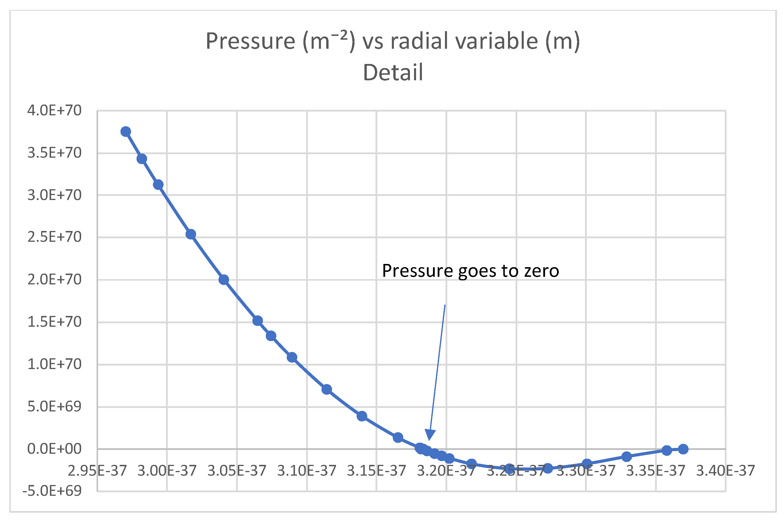
We can use the results of numerical integration to map the pressure profile as a function of the proper radial distance from the center of the electron. As shown in the figure below the pressure falls off within the near zone until it drops to zero at the surface, Figure 2. The solution is reminiscent of the external metric of a charged black hole (Reissner-Nordstrom metric).

One may ask if general relativity is valid at such short lengths. The existence of black holes and the cosmic background radiation offer evidence to the contrary.

If we substitute ${\eta }_e$ from Eq. (26) into Eq. (4) we get a mass independent of the electron mass. We call it the universal mass ${\mu }_{*}$.

$${\mu }_{*}={\displaystyle \frac{1}{2}}\sqrt{{\displaystyle \frac{\alpha }{4\pi }}{\displaystyle \frac{\hslash c}{G}}}={\displaystyle \frac{1}{2}}\sqrt{{\displaystyle \frac{\alpha }{4\pi }}}{m}_P$$

(33)

in terms of the Planck mass $m_P.$ The Planck mass also appears naturally.

Simplifying the result

$${\mu }_{*}={\displaystyle \frac{1}{2}}\sqrt{{\displaystyle \frac{1}{4\pi }}}\sqrt{{\displaystyle \frac{e^2}{G}}}$$

(34)

dependent on e and G alone and independent of ℏ and c. Numerically

$${\mu }_{*}\approx {10}^{17}GeV$$

(35)

By comparison the mass obtained in [8] is ${10}^{18}$GeV. This result is remarkable for several reasons. Since ${\mu }_{*}$ is enormously larger than the physical mass m it cannot be the corrected mass. Furthermore ${\mu }_{*}$ is independent of mass; it is solely in terms of the fundamental constants e and G . Since it depends on $e^2$ it is also independent of the sign of the charge. The inescapable conclusion is that the result is a general result applicable to all charged particles irrespective of the mass and sign of the charge.

Although our goal was to derive the corrected electron mass we have found instead a mass that applies to all charged particles. A possible interpretation is that ${\mu }_{*}$ is the universal mass.

These observations also apply to the radius $r_{*}$ since it too is independent of mass, and is in terms of the fundamental constants $G,$c and e .

The value of ${\mu }_{*}$ is close to the GUT energy $\left({10}^{16}GeV\right)$ where it is conjectured that all forces except gravity merge. It would appear that all forces, including gravity, merge at ${10}^{17}GeV$ . Since the merged or unified field depends only on e and G it would be consistent to call it the electrogravity field.

Why the discrepancy between the theoretical energy and the measured energy ($0.5Mev)$? We will provide an explanation in the next section.

Since the electrogravity field energy is independent of ℏ one may also conclude that the unified field is not quantized but is a continuum. This is a serendipitous result.

The universal mass is exact. The integral converges to an exact value. Physical laws remain unaltered.

The momentum upper limit is

$$k^{max}={\displaystyle \frac{\hslash }{r_e}}$$

(36)

We reiterate that this is a self-regulating mechanism since if k creeps up beyond $k^{max}$ it engenders a proportional reaction from the metric such that the system reverts to a state of equilibrium. The equilibrium is stable.

At $r=4\times {10}^{-37}m$ where the two competing pressures are equal; the pressures are

$${10}^{79}{m}^{-2}$$

(37)

in geometric units, or ${10}^{123}N/m^2$ in standard units. Evidently the electron surface is highly stressed; the pressure is ≈${10}^{118}$ atmospheres on the surface. By comparison the pressure inside neutron stars is merely ≈${10}^{30}$ atmospheres.

At this value the outward pressure due to the energy density of self-interaction equals the inward pressure of the curved metric.

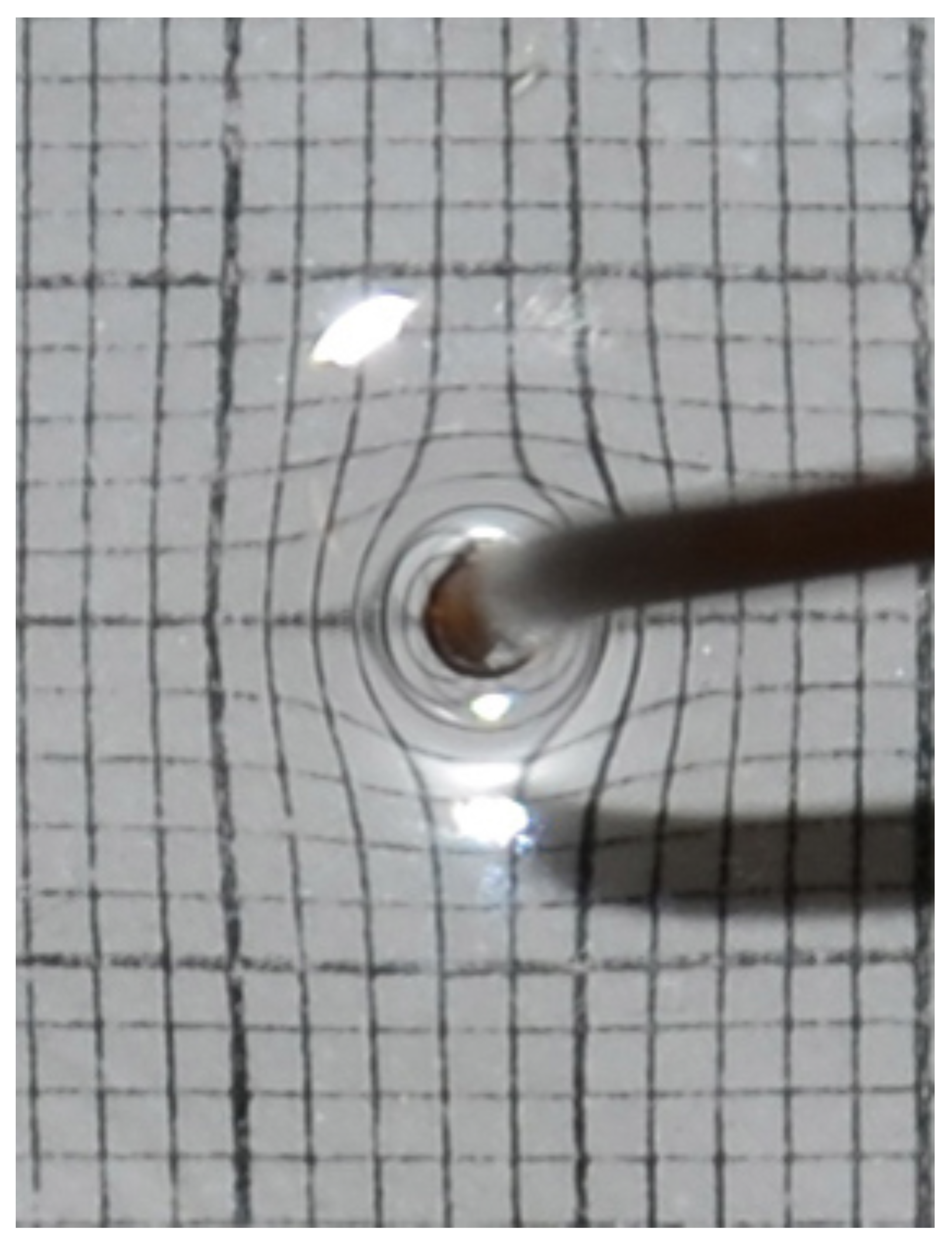
Pictorially, the distorted metric in the vicinity of the electron looks like this photo-representation Figure 3:

The inward pressure is a consequence of the distorted metric.

1.7. Speed of Excitations

In this section we calculate the speed of excitations v within the electron. These are longitudinal excitations of the electrogravity field. Using Eq. (24) and Eq. (15)

$${\displaystyle \frac{v}{c}}=\sqrt{{\displaystyle \frac{dP/d\eta }{d\rho /d\eta }}}$$

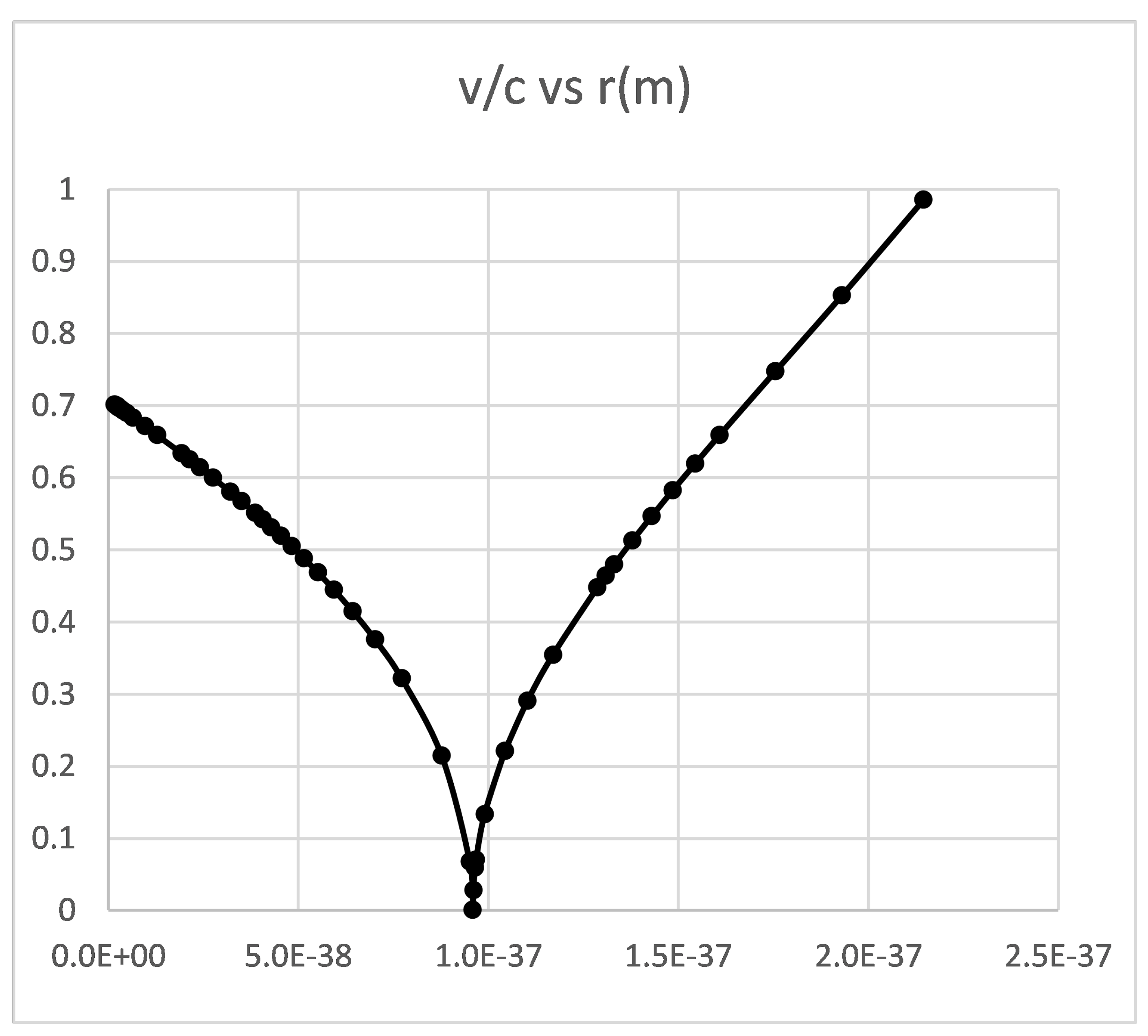
The graph in Figure 4 shows $v/c$ as a function of the proper distance r from the center. These are longitudinal waves within the near zone.

1.7.1. Discrepancy Between Theoretical and Measured Masses

In this section we resolve the apparent discrepancy between measured and theoretical values of the mass of electrons. The discrepancy is of the order of ${10}^{26}/0.511\times {10}^6\approx {10}^{21}$.

The measurement protocol entails a two-step process. Using the Thomson method we first measure the charge to mass ratio $e/m$ then separately measure e using the Millikan oil drop method. The electron mass is calculated from the ratio of the two. In measuring $e/m$ we rely on Thomson’s experiment where an electron beam is launched into a region of uniform magnetic field. The acceleration associated with the Lorentz force on the moving electron is then equated to $F=ma$ from which the ratio $e/m$ is calculated.

In the co-moving frame of the electron the magnetic field appears as an electric field E. The force on the charge e due to E is heavily reduced by the intervening metric surrounding the electron. We identify this mechanism which explains the discrepancy between theoretical and measured masses. Thus renormalization is neither necessary nor justified.; there is perfectly cogent explanation behind the discrepancy.

The external electric field (due to the co-moving frame) close to the surface of the electron can be calculated. We use the external field of a charged black hole - Reissner-Nordstrom metric to emulate the field of the electron, How is the external comoving field altered in a Riessner-Nordstrom metric?

We use results derived by Bini, Geralico and Ruffini[10]. Their work shows that the gravitational and electric fields interact, altering both - "electromagnetically induced gravitational perturbation" as well as the "gravitational induced electromagnetic perturbation".

Using values typical in a Bainbridge $e/m$ apparatus the E-field in the comoving frame of the circulating electron is $\approx {10}^{4}V/m$ at a distance of $0.1m.$ We can use the method of images to compute the location of an image charge. The image charge is at the center of the circle of the circulating electron beam.

Thus we achieve a geometry of an electron whose external field is represented by the Reissner-Nordstrom metric. The image charge and its electric field interacts with the electron. The geometry reproduces the model used in the paper referred to. We can use the results directly (Eqs. 14, 15 and 16) [10].

We find that the external electric field (due to the image charge, and indirectly due to the relative motion between electron and external magnetic field) is heavily attenuated in the vicinity of the electron. The result is a much smaller force and concomitant smaller acceleration.

The net effect is a much smaller measured electron mass when the ratio $e/(e/m)$ is calculated.

We show this explicitly. Denoting the external field by $F_{ext}$, the altered field as $F_{th}$, the experimental mass as $m_{ex}$, and the altered mass as $m_{th}$ we may write the ratios

$$\begin{array}{ccc}\hfill {\displaystyle \frac{F_{ext}}{F_{th}}}& =& {\displaystyle \frac{m_{ex}a}{m_{th}a}}\hfill \end{array}$$

(38)

$$\begin{array}{ccc}\hfill m_{th}& =& m_{ext}{\displaystyle \frac{F_{th}}{F_{ext}}}\hfill \end{array}$$

(39)

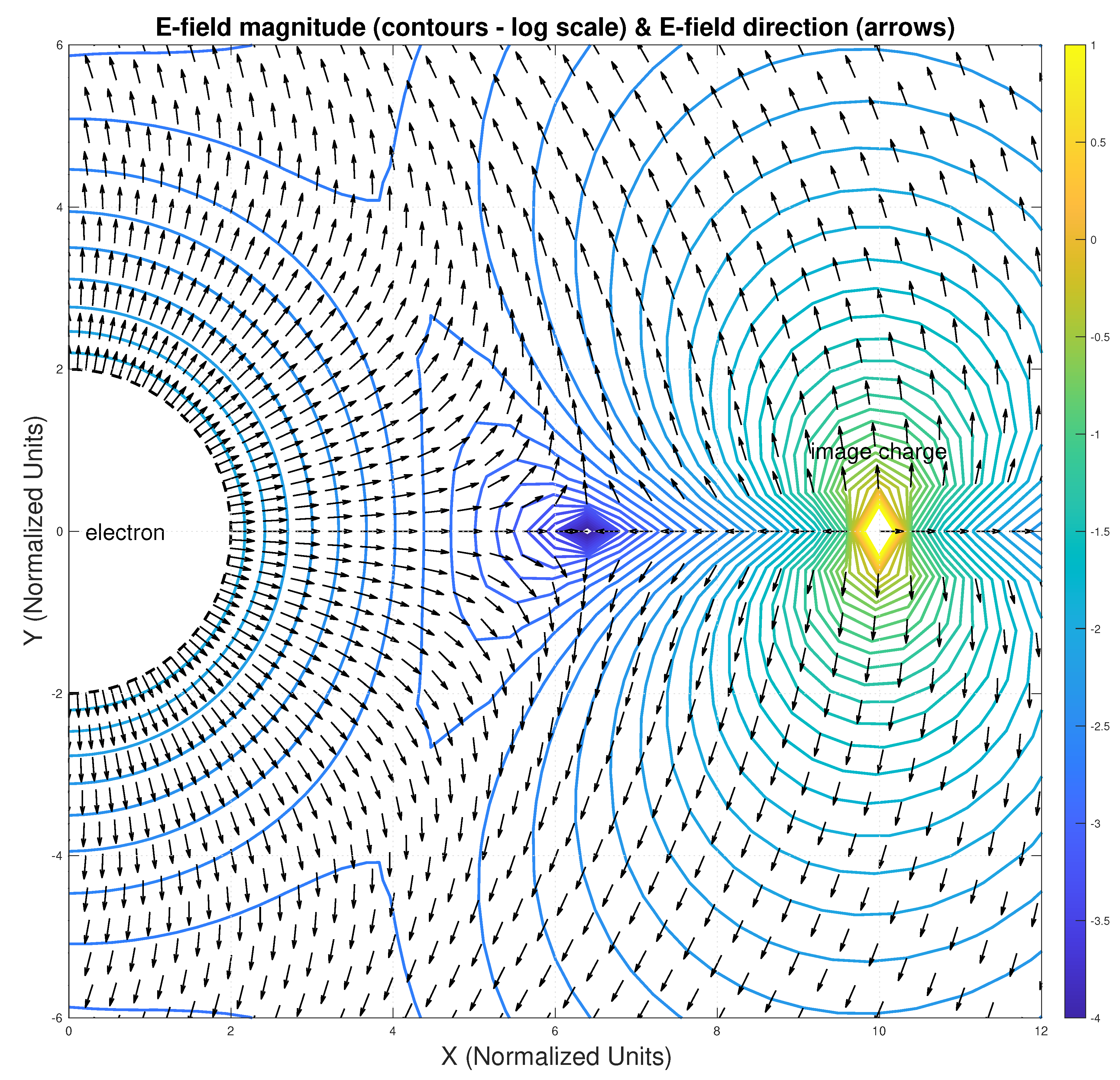
In Figure 5 we show the vector field graph of the electric fields from both the electron and the source charge in the external Reissner-Nordstrom metric of the electron. There are two source charges. The half disc on the left is the electron: the image charge appears as a diamond on the right. Clearly the field directions change sign in between. Near $r\approx 7.5\times {10}^{-7}m$ the image field is close to zero or $\approx {10}^{-21}.$

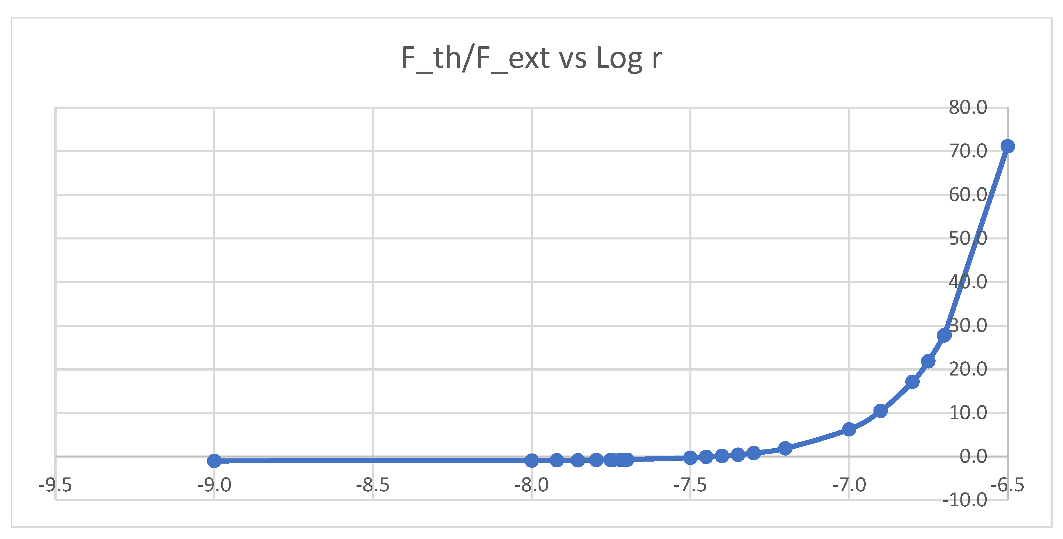
In Figure 6 we show a graph of the ratio of the theoretical field and the unaltered field agaimst the radial coordinate. It shows the inflection point of the electric field at a precise location, corroborating what is seen in the vector field graph.

1.8. Conclusion

Although we have calculated the metric for electrons, we note that all stable particles with the same charge (e) have the same mass as well.

Previously there have been attempts to introduce gravitation to remove infinities in the self-energy correction to the electron mass [8], however, this work demonstrates the existence of an auto-generated curved metric in the vicinity of an electron as well as an explicit computation of the upper limit on the momentum vector. The self-energy integral is shown to be finite; infinities in the perturbative expansion have been removed. The series converges. The mass correction has an exact value, free of infinities.

We have demonstrated that gravitation is essential to stabilize the electron. Competing pressures from the electromagnetic and gravitational fields auto-stabilize the electron. We have identified the Poincare’ stress.

We calculate from first principles the radius of the electron as well as the Planck length and Planck mass. In deriving the electron radius and mass we identify the mechanism (inward pressure of the induced metric) that stabilizes the electron. The mass correction is close to the GUT scale - an unexpected result.

We dispense with the theory that the electron is made up of a bare mass plus a radiative mass. It is evident that the electron is a stable configuration of the electrogravity field.

We have also demonstrated that the electrogravity field being independent of ℏ, is continuous. Furthermore, the fields merge at ${10}^{17}GeV$, consistent with the conjectured energy in Grand Unified Theories $\left({10}^{16}GeV\right)$.

We have provided an explanation for the discrepancy of ${10}^{21}$ between measured and theoretical values of the electron mass.

We were able to calculate the speed of excitations of the electrogravity field within the electron and discover that the internal structure is inhomogeneous - consisting of a hard shell enclosing a softer core.

Furthermore instead of using dimensional analysis to derive the Planck length and mass we show that both are a consequence of merging quantum electrodynamics with gravitation.

The solution we obtain is exact; since it is independent of mass it is valid for strong fields as well.

1.9. Acknowledgments

We are grateful to Mark Bocko for preparing the vector field graph Figure 6, to Belal Baaquie who identified the connection between Eq. (28) and the Planck length, to Roberto Onofrio for continuous encouragement and advice, to the late Adrian Mellissinos for his interest in this work; and for support from my wife Maureen Patricia and daughter Kim Samar. A special thanks to Professors Habauka Kwaambwa and Percy Chimwamurombe for their continuing hospitality at the Namibia University of Science and Technology.

1.10. Appendix

Derivation of Eq. (1.1): start by using the identity: we follow Feynman [5].

$${\displaystyle \frac{1}{ab}}={\int }_0^1{\displaystyle \frac{dx}{{\left[ax+b\left(1-x\right)\right]}^2}}$$

(40)

Define two quantities

$$k^2-2p·k\equiv a;k^2\equiv b$$

(41)

Then

$${\displaystyle \frac{1}{\left(k^2-2p·k\right)k^2}}={\int }_0^1{\displaystyle \frac{dx}{{\left[\left(k^2-2p·k\right)x+k^2\left(1-x\right)\right]}^2}}={\int }_0^1{\displaystyle \frac{dx}{{\left[k^2-2p·kx\right]}^2}}$$

(42)

So Eq. (1.1) becomes

$$\Delta m={\displaystyle \frac{4\pi e^2}{2mi}}{\int }_{-\infty }^{\infty }{\displaystyle \frac{\tilde{u}\left(2m+2k\right)u}{k^2-2\overrightarrow{p}·\overrightarrow{k}}}{\displaystyle \frac{d^{4}k}{{\left(2\pi \right)}^4}}{\displaystyle \frac{1}{k^2}}$$

(43)

$$d^{4}k=d\omega d^3\overrightarrow{K};k^2-2p·kx={\omega }^2-\left({\overrightarrow{K}}^2+2p·kx\right)$$

(44)

Let $xp\equiv p$ then

$$\Delta m={\displaystyle \frac{4\pi e^2}{2mi}}{\int }_{-\infty }^{\infty }{\displaystyle \frac{\tilde{u}\left(2m+2k\right)u}{\left[{\omega }^2-\left({\overrightarrow{K}}^2+2p·kx\right)\right]}}{\displaystyle \frac{d\omega d^3\overrightarrow{K}}{{\left(2\pi \right)}^4}}{\displaystyle \frac{dx}{k^2}}$$

(45)

Do the $\omega$ integral first using residues, and for $\epsilon \ll L+{\overrightarrow{K}}^2$ :

$${\int }_{-\infty }^{\infty }{\displaystyle \frac{d\omega }{\left[{\omega }^2-i\epsilon +\left({\overrightarrow{K}}^2+2p·k\right)\right]}}={\displaystyle \frac{-2\pi i}{2\sqrt{{\overrightarrow{K}}^2+2p·k}}}\equiv {\displaystyle \frac{-2\pi i}{2\sqrt{{\overrightarrow{K}}^2+L}}}$$

(46)

Since the only contribution to the integral comes from the pole we choose the limits as $\pm \infty$ for $\omega$. Take derivatives with respect to L on both sides:

$${\int }_{-\infty }^{\infty }{\displaystyle \frac{d\omega }{{\left[{\omega }^2-i\epsilon +\left({\overrightarrow{K}}^2+2p·k\right)\right]}^2}}={\displaystyle \frac{\pi i}{2{\left({\overrightarrow{K}}^2+2p·k\right)}^{3/2}}}$$

(47)

$${\int }_0^{\infty }{\displaystyle \frac{d\omega }{{\left[{\omega }^2-i\epsilon +\left({\overrightarrow{K}}^2+2p·k\right)\right]}^2}}={\displaystyle \frac{\pi i}{4{\left({\overrightarrow{K}}^2+2p·k\right)}^{3/2}}}$$

(48)

The remaining integral is

$$\begin{array}{ccc}\hfill {\displaystyle \frac{\pi i}{4}}{\int }_0^K{\displaystyle \frac{4{\pi }^2{K}^{2}dK}{{\left(K^2+L\right)}^{3/2}}}& =& i{\pi }^3{\left[{\displaystyle \frac{-K}{\sqrt{K^2+L}}}+ln\left(K+\sqrt{K^2+L}\right)\right]}_0^K\hfill \end{array}$$

(49)

$$\begin{array}{ccc}& =& i{\pi }^3\left[{\displaystyle \frac{-K}{\sqrt{K^2+L}}}+ln\left({\displaystyle \frac{K+\sqrt{K^2+L}}{\sqrt{L}}}\right)\right]\hfill \end{array}$$

(50)

The last integral is over x. Insert x back into the integral

$${\int }_0^1\left[{\displaystyle \frac{-K}{\sqrt{K^2+2xp·k}}}+ln\left({\displaystyle \frac{K+\sqrt{K^2+2xp·k}}{\sqrt{2xp·k}}}\right)\right]dx$$

(51)

The two integrals are

$${\int }_0^1\left[{\displaystyle \frac{-K}{\sqrt{K^2+2xp·k}}}\right]dx={\left[{\displaystyle \frac{-2K\sqrt{K^2+2xp·k}}{2p·k}}\right]}_0^1={\displaystyle \frac{-K\sqrt{K^2+2mck}}{mck}}+{\displaystyle \frac{1}{mc}}$$

(52)

$$\begin{array}{ccc}& & {\int }_0^{1}ln\left({\displaystyle \frac{K+\sqrt{K^2+2xp·k}}{\sqrt{2xp·k}}}\right)dx\hfill \end{array}$$

(53)

$$\begin{array}{ccc}& =& \left[{\displaystyle \frac{k\sqrt{k^2+2mck}}{2mck}}+ln\left({\displaystyle \frac{\sqrt{k^2+2mck}+k}{\sqrt{2mck}}}\right)\right]-{\displaystyle \frac{k^2}{2mck}}\hfill \end{array}$$

(54)

Substituting for $k=\hslash \kappa$ Eq. (3) and $\eta \equiv \hslash /2mcr={\lambda }_C/4\pi r$ the mass correction is:

$$\Delta m\equiv \mu \left(r\right)={\displaystyle \frac{\alpha m}{2\pi }}\left[-{\displaystyle \frac{\eta }{2}}\sqrt{1+{\displaystyle \frac{1}{\eta }}}+\eta +ln\left\{\sqrt{\eta }\left(\sqrt{1+{\displaystyle \frac{1}{\eta }}}+1\right)\right\}\right]$$

For a stationary electron $p=mc$.