
Submitted:
24 February 2025
Posted:
25 February 2025
You are already at the latest version
Abstract
The equilibrium equation for a variable thickness flywheel is approximated analytically, assuming that the flywheel’s thickness varies linearly and as smoothly as to neglect it. The solution shows an accurate approximation of maximum radial and tangential stresses, with respect to finite element method, for a wide range of outer/inner thickness relation. The performance of the results was quantified with the Pearson correlation factor, the mean absolute percentage error, and the relation between the maximum stresses calculated with FEA and the results obtained with the obtained solution.
Keywords:
Variable thickness flywheel
; FEA
; Equilibrium equation
; Analytical approximation
; Mean absolute percentage error
1. Introduction
Calculating the stress of variable-thickness flywheels using an equation is of absolute importance in mechanical engineering. Most flywheel cross sections are designed and optimized using FEA software as a consequence of the lack of an equation to determine the stresses.
Flywheels have multiple applications, such as space technology, renewable energy and transportation systems, and power networks, among others [1,2,3,4]. Flywheels are the main component of flywheel energy storage systems (FESS), an electromechanical device that converts kinetic rotational energy into electrical energy [2]. FESS are widely used for their flexibility to store energy and later convert and manipulate it [2]. They offer high efficiency, large amounts of instantaneous power, fast response, low maintenance costs, long-lasting services, in addition to multiple environmental benefits [1,3,4].
1.1. Background
In analyzing and designing an FESS, optimizing the size, shape, and topology of the flywheel is of great value, since these parameters are directly related to the energy storage capacity of the FESS [2]. There are many researchers who investigate the analysis and optimization of flywheel size, shape, and topology [5,6,7]. On the one hand, most of them use numerical methods, such as the finite element method (FEM), or finite element analysis (FEA). Kailisan [4], for example, performed an FEA on a composite flywheel that integrates carbon fiber and a steel spline ring to limit the tangential stress that would allow high-speed operation. The authors show positive results, including the fact that, because of the steel rings, centrifugal growth would not induce the rotor parts to separate. A shape optimization FEM was implemented by Jiang [6]. The method relies on the parametric geometry modeling method and the downhill simplex method. The results show that the energy density and working safety performance could be significantly improved by implementing this shape optimization method. Furthermore, Jiang [7] implemented the variable density method and FEM to optimize the topology of a flywheel for energy density. The results show a 56.7% increase in the energy density of a constant thickness flywheel. Gao [8] presents a novel FESS, with the flywheel design being the main novelty. It consists of a double hub and rim that yields a mass reduction and an increase in inertia. The results show no separation between the rim and the dual hubs at high speeds. Kale [5] introduces an optimization method that eliminates the constraint of arbitrarily large volumes, used in traditional kinetic energy methods. The method, based on the maximization of specific energy, achieved a 15.8% increase in specific energy, compared to the kinetic energy method.
On the other hand, there are researches that have proposed analytical solutions for variable thickness flywheels. But this is not an easy task. Wen [9], for example, analyzed the stresses in an anisotropic flywheel based on plane stress. After the radial and tangential stresses were obtained, the location of the maximum radial stress was derived using the extreme point method and calculated using the Newton method. The results show a fine approximation which could be used in the design of composite flywheels. To the best of our knowledge, at the time of developing this work, the equilibrium equation for a flywheel with a linearly variable thickness had not been solved. Although Semsri [2] uses the solution provided by Ugural [10] to analyze a conical flywheel, Ugural’s solution is clearly and explicitly provided for a hyperbolic profile.
In the next section, the equilibrium equation is solved, assuming that the flywheel’s thickness varies linearly. A compact and easy-to-handle equation is given and further analyzed. The equation obtained was used to compute the stresses developed in the flywheel, and these results were compared with the FEA results. In Section 3, the results of Section 2 are discussed.
2. Methodology
The design of a constant thickness flywheel is based mainly on two stresses: a radial stress, , and a tangential one, . is given by [2]
and by [2]
where
is the outer radius of the flywheel,
is the inner radius of the flywheel,
r is the radial distance at which the stress is to be computed,
is the flywheel’s material’s Poisson ratio,
is the density of the flywheel material and
is the flywheel’s angular velocity.
In Figure 1 the results of an FEM analysis, performed in a commercial FEA software, are shown. It can be seen that the results of the simulation converge with those computed analytically with Eq. 1 and 2. Figure 1a shows , Figure 1b shows , and Figure 1c shows the comparison between the simulation results and Eq. 1 and 2. Figure 1c shows the behavior of and , using data from Table 1. It can be seen that the total stress, , is much more influenced by . The maximum stress is about 14 kPa.
Although the stresses for a constant-thickness flywheel are relatively easy to find, the stresses in a variable-thickness flywheel are not. In this study, the main goal was to find an expression that would help to calculate the stresses in a variable-thickness flywheel. This is not an easy task, ever since there is no equation to compute the stresses in most variable thickness shapes. To find such an equation, the analysis started from the stress function [11] given by
Equation 3 is clearly not linear when t is described by a polynomial, as in the case of a conical flywheel. Therefore, it is necesary to solve Eq. 3 by other means. In Eq. 3, the fourth term derives from the rotational body force. That is, when such a term is considered, Eq. 3 is not homogeneous, while if it is not, then Eq. 3 is homogeneous.
The most simple case for a variable-thickness flywheel is when the thickness varies linearly along the radius. That being said, lets consider t given by
Now, if the variation of t is small, that is, if is small, then the last term in Eq. 3 can be neglected and it becomes:
Since the last term in Eq. 5 yields to a fourth degree polynomial, considering Eq. 4, the particular solution to Eq. 5, , should have the form
Upon substitution of Eq. 6 and 4 in Eq. 5, , , and . Therefore, is
As for the homogeneous solution, , it is noted that the homogeneous form of Eq. 5 is the same as the homogeneous one for a constant thickness flywheel [11]. Therefore, is
where and are determined from the boundary conditions. In this case, at and .
Upon applying boundary conditions, and are given by
and
with .
If the flywheel’s thickness is considered to vary linearly along the radius, as defined by Eq. 4, then A and B can be defined as functions of , , internal thickness, , and outer thickness, , as
and
With Eq. 8 and Eq. 9 through 12, the relation between the stresses in the flywheel and its geometry is explicit.
To validate Eq. 8, an FEM analysis was performed in an FEM software and the results were compared with those obtained with Eq. 8 and are presented in Figure 2 and Figure 3. The results of Figure 2 were obtained using the parameters given in Table 2. From Table 2 it is evident that the flywheel’s thickness variation is too small. Therefore, an analysis was performed to determine the interval of values for the thickness relation , for which Eq. 8 is valid. In other words, for what values of does Eq. 8 give an acceptable approximation of and in a variable-thickness flywheel with t given by Eq. 4.
Both and were obtained with FEA along two lines, line 1 and line 2, depicted in Figure 2a, for . Furthermore, Figure 2b shows the Pearson correlation factor, P, between and obtained with FEA and Eq. 8. The figure shows a high correlation for both stresses in both lines, between Eq. 8 and FEA; Figure 2c shows the mean absolute percentage error (MAPE). It shows that the MAPE behaves similarly in the four cases. However, it is higher for ; Figure 2d shows the ratios between the maximum stresses obtained with FEA in lines 1 and 2 and those obtained with Eq. 8. In Figure 2d, it is noticeable that Eq. 8 offers a better approximation for , between 0.8973 and 1.0658, at line 1 than for , between 0.6965 and 1.0133, with respect to the values determined with FEA. For the stresses in line 2, Eq. 8 offers a better approximation for , with values between 0.9958 and 1.0761, than for , with values between 0.8589 and 1.0436, with respect to the values determined with FEA. Additionally, Figure 3a shows the ratios of the maximum stresses in Line 2 and the maximum stresses at Line 1. It is noted that the relation between the maximum at Line 2 and at Line 1 increases from 1.0248, at , to 1.4297, at . Unlike the relation for , which decreases from 1.0083, at , to 0.9958, at . Furthermore, Figure 3b and Figure 3c show the results for , at Line 2, and , at Line 1, from the FEA compared with the ones obtained with Eq. 8, respectively. Figure 3a and Figure 3b highlight that, although the maximum stresses are fine approximations, the MAPE is considerably high, specially in for . All results from Figure 2 and Figure 3 are presented in function of .
3. Discussion
In this study, the solution of the equilibrium equation for a variable-thickness flywheel, Eq. 3, is based on the assumption that the flywheel thickness varies smoothly, so that , and is given by Eq. 4. This assumption simplifies Eq. 3 and yields Eq. 5. With the assumption that , the solution to Eq. 5 is an easy task. The solution to Eq. 5 is basically the solution for a flywheel of constant thickness plus the term , which accounts for the thickness variation. In fact, when the thickness is constant, and , leading to Eq. 1 and 2.
The validation analysis exhibits a high correlation between the solution, given by Eq. 8, and the results obtained from FEA, for , Figure 3b. However, P should not be considered as the only way to quantify how good an approximation Eq. 8 is, but rather consider that both solutions, FEA and Eq. 8, behave very much alike within .
Furthermore, Figure 3c shows that the MAPE between the results, although exhibiting very high values of P, begins to increase as the thickness relation increases. Additionally, in Figure 3d is noted that Eq. 8 offers an excellent approximation for both maximum values of and within . Although the maximum varies significantly from Line 2 to Line 1, that is, along the thickness of the flywheel, Eq. 8 is an excellent approximation for the maximum on Line 2, the line at which the designer is more interested in determining , since that is where the maximum is. Alternatively, Eq. 8 offers a better approximation of maximum at Line 1 than at Line 2. Unlike , the variation of along the thickness of the flywheel is too small and could be neglected. Nonetheless, it is important to keep in mind that it does varies and it is higher at Line 1 than at Line 2. However, it can be concluded that Eq. 8 is a very good approximation for maximum and within .
Figure 3.
(a) Relation of maximum stress at Line 2 and Line 1. (b) computed with FEA and Eq. 8. (c) computed with FEA and Eq. 8.
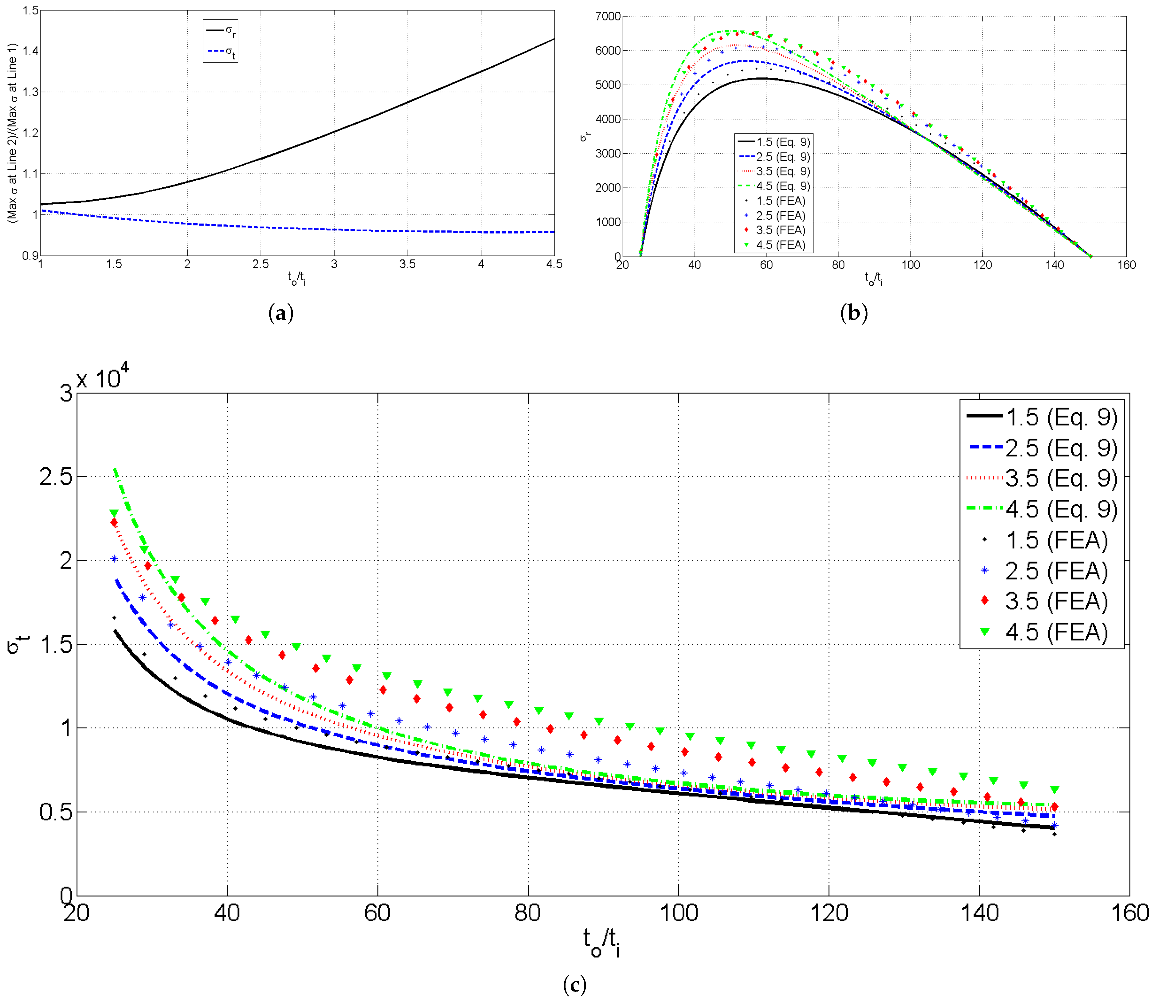
Although this solution was developed for t given by Eq. 4, the solution method could be applied to higher-order polynomials of t, as a consequence of Lagrange’s mean value theorem. That is, the solution for maximum stresses would be valid within a 10% variation from FEM as long as .
Equation 8 was observed to approximate better than , Figure 2 and Figure 3. That is attributed to the fact that is obtained with the derivative of F, unlike , which is obtained directly from F. Since F is an approximation, its derivative will lose accuracy and so will .
Furthermore, although the maximum and are well approximated, exhibits a quantitatively considerable MAPE, higher than 10%, for , and higher than 15% for . This is a very important information to bear in mind when using Eq. 8 to design a variable-thickness flywheel. Maximum stresses will be within a fine approximation for high values of , but the higher the thickness relation, the higher a design factor, proportional to the MAPE, should be included in the calculation of to avoid under-sizing the flywheel. Finally, it is important to highlight the fact that a high value of is unusual and the flywheel could be divided into a convenient number of elements and treat every element independently, as recommended by Timoshenko [11].
4. Conclusions
In this paper, the equilibrium equation for a variable-thickness flywheel is approximated analytically, assuming that the flywheel’s thickness varies smoothly, as smoothly as to take . Another assumption was that the thickness varies linearly, that is, given by a first-degree polynomial. However, the solution method could also be applied to polynomials of a higher degree t, as long as is negligible or as long as .
The solution shows an accurate approximation of the maximum radial and tangential stress, with respect to FEA, for a wide range of .
Developing this approximation to obtain the stresses in a variable-thickness flywheel gives the mechanical designer an easier, faster, and reliable way to calculate the stresses in the flywheel, without recurring to FEA. Additionally, providing an equation that explicitly relates the stresses in the flywheel and its geometry would allow an easier way to optimize its size, cross section, and topology.
Author Contributions
M. G.: Conceptualization, methodology, investigation, data curation, writing – original draft, writing – review and editing, visualization, supervision, project administration.O. O.: Writing-original draft, visualization, project administration, supervision. O. C.: Methodology, conceptualization, methodology. J. U.: Writing–review and editing. A. B.: Visualization, Supervision.
Data Availability Statement
Data generated during the current study are available from the corresponding author on reasonable request.
Acknowledgments
The authors would like to thank the National Council for Humanities, Sciences and Technologies (CONAHCYT, Consejo Nacional de Humanidades, Ciencias y Tecnologías) for the postdoctoral grant key BP-PA-20230511211217474-4861409.
Conflicts of Interest
The authors certify that they have NO affiliations with or participation in any organization or entity with any financial interest (such as honoraria; educational grants; participation in speakers’ bureaus; membership, employment, consultancies, stock ownership or other equity interest; and expert testimony or patent-licensing arrangements), or nonfinancial interest (such as personal or professional relationships, affiliations, knowledge or beliefs) in the subject matter or materials discussed in this work.
Abbreviations
The following abbreviations are used in this manuscript:
| FESS | Flywheel energy storage system |
| FEM | Finite element method |
| FEA | Finite element analysis |
| MAPE | Mean absolute percentage error |
References
- Xu, K.; Guo, Y.; Lei, G.; Zhu, J. A Review of Flywheel Energy Storage System Technologies. Energies 2023, 16. [Google Scholar] [CrossRef]
- Semsri, A. Experimental Design of Flywheel Rotor with a Flywheel Energy Storage System for Residential uses. International Energy Journal 2023, 23. [Google Scholar]
- Acarnley, P.P.; Mecrow, B.C.; Burdess, J.S.; Fawcett, J.N.; Kelly, J.G.; Dickinson, P.G. Design Principles for a Flywheel Energy Storage for Road Vehicles. IEEE Transactions on Industry Applications 1996, 32, 1402–1408. [Google Scholar] [CrossRef]
- Kailasan, A.; Dimond, T.; Allaire, P.; Sheffler, D. Design and Analysis of a Unique Energy Storage Flywheel System—An Integrated Flywheel, Motor/Generator, and Magnetic Bearing Configuration. Journal of Engineering for Gas Turbines and Power 2015, 137, 042505. Available online: http://arxiv.org/abs/https://asmedigitalcollection.asme.org/gasturbinespower/article-pdf/137/4/042505/6165248/gtp_137_04_042505.pdf. [CrossRef]
- Kale, V.; Aage, N.; Secanell, M. Stress Constrained Topology Optimization of Energy Storage Flywheels Using a Specific Energy Formulation. Journal of Energy Storage 2023, 61, 106733. [Google Scholar] [CrossRef]
- Jiang, L.; Zhang, W.; Ma, G.J.; Wu, C.W. Shape Optimization of Energy Storage Flywheel Rotor. Structural and Multidisciplinary Optimization 2016, 55, 739–750. [Google Scholar] [CrossRef]
- Jiang, L.; Wu, C.W. Topology Optimization of Energy Storage Flywheel. Structural and Multidisciplinary Optimization 2016, 55, 1917–1925. [Google Scholar] [CrossRef]
- Gao, J.; Zhao, S.; Liu, J.; Du, W.; Zheng, Z.; Jiang, F. A Novel Flywheel Energy Storage System: Based on the Barrel Type with Dual Hubs Combined Flywheel Driven by Switched Flux Permanent Magnet Motor. Journal of Energy Storage 2022, 47, 103604. [Google Scholar] [CrossRef]
- Wen, S. Analysis of Maximum Radial Stress Location of Composite Energy Storage Flywheel Rotor. Archive of Applied Mechanics 2014, 84, 1007–1013. [Google Scholar] [CrossRef]
- Ugural, A.C.; Fenster, S.K. Advanced Mechanics of Materials and Applied Elasticity; Pearson, 2020. [Google Scholar]
- Timoshenko, S.; Goodier, J. Theory of Elasticity; McGraw-Hill, 1951. [Google Scholar]
Figure 1.
Results of a stress analysis in Abaqus. The figure shows radial stress (a), tangential stress (b), and the comparison between the results from the FEA and Eq. 1 and 2 (c).
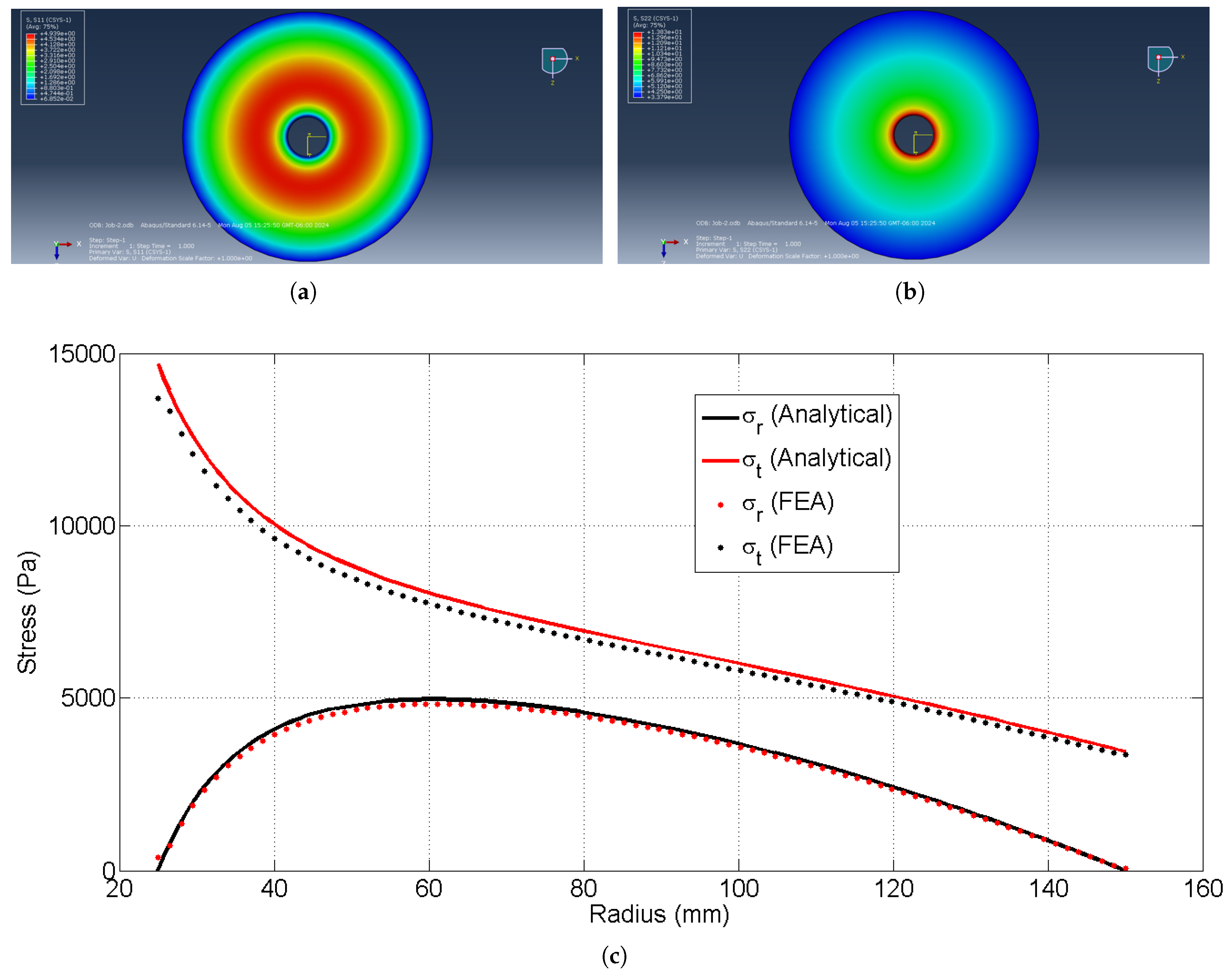
Figure 2.
(a) Lines 1 and 2 where and were computed. (b) Pearson correlation factors between FEA and Eq. 8. (c) MAPE between FEA and Eq. 8. (d) Relation between maximum . and obtained with FEA and Eq. 8.
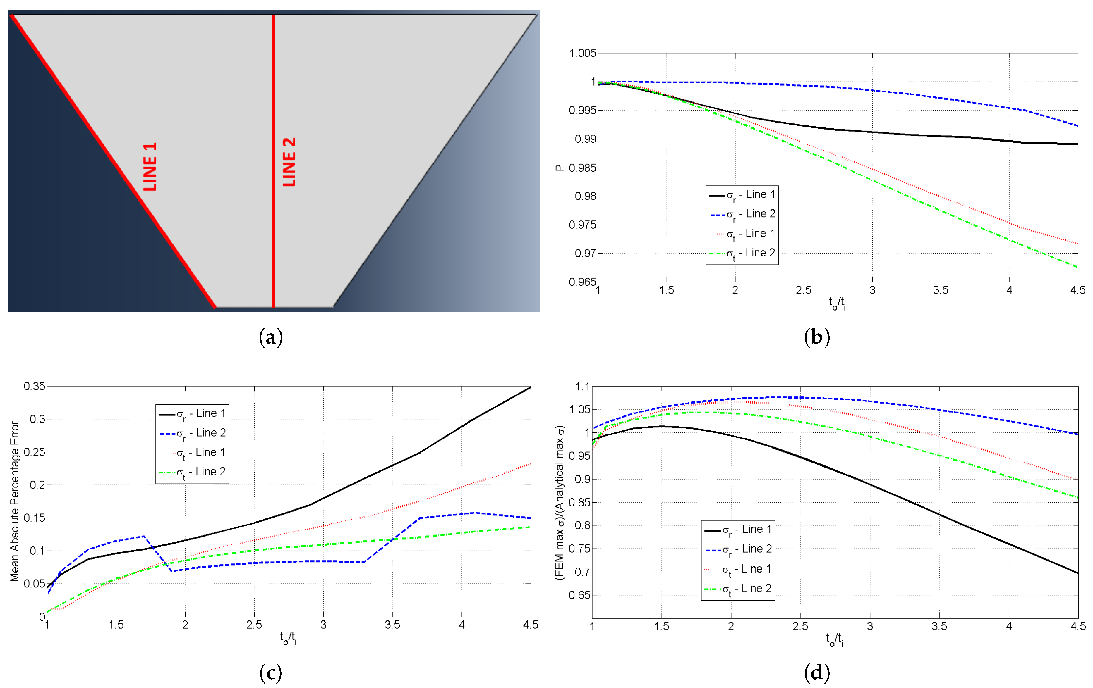

Table 1.
Parameters used for computing stresses at Figure 1
Table 1.
Parameters used for computing stresses at Figure 1
| Parameter | Numerical value |
|---|---|
| 25 mm | |
| 150 mm | |
| 0.3 | |
| 7850 kg/ | |
| 9.84 rad/s |
Table 2.
Parameters used for computing stresses at Fig. Figure 2
Table 2.
Parameters used for computing stresses at Fig. Figure 2
| Parameter | Numerical value |
|---|---|
| 25 mm | |
| 150 mm | |
| 0.3 | |
| 50 mm | |
| 55 mm | |
| 7850 kg/ | |
| 9.84 rad/s |
Disclaimer/Publisher’s Note: The statements, opinions and data contained in all publications are solely those of the individual author(s) and contributor(s) and not of MDPI and/or the editor(s). MDPI and/or the editor(s) disclaim responsibility for any injury to people or property resulting from any ideas, methods, instructions or products referred to in the content. |
© 2025 by the authors. Licensee MDPI, Basel, Switzerland. This article is an open access article distributed under the terms and conditions of the Creative Commons Attribution (CC BY) license (http://creativecommons.org/licenses/by/4.0/).
Copyright: This open access article is published under a Creative Commons CC BY 4.0 license, which permit the free download, distribution, and reuse, provided that the author and preprint are cited in any reuse.


