Submitted:
24 February 2025
Posted:
25 February 2025
You are already at the latest version
Abstract
Blood concentrations of essential trace elements can be used to diagnose conditions and diseases associated with excess or deficiency of these elements. Inductively coupled plasma mass spectrometry (ICP-MS) has been employed for such measurements, but maintenance and operation costs are high. XRF detectability in cutaneous blood of iron (Fe), copper (Cu), zinc (Zn), and selenium (Se) was assessed as alternative to ICP-MS. Three phantoms were made up of two polyoxymethylene (POM) plastic cylindrical cups of 0.6-mm and 1.0-mm thick walls and a 5.3-mm diameter POM cylindrical insert. Six water solutions of Fe in 0 to 500 mg/L and Cu, Zn, and Se in 0 to 50 mg/L concentrations, were poured into the phantoms to simulate x-ray attenuation of skin. Measurements using an integrated x-ray tube and polycapillary x-ray lens unit generated 24 calibration lines. Detection limit intervals in mg/L were: (36, 100), (14, 40), (3.7, 10), and (2.1, 3.4) for Fe, Cu, Zn, and Se, respectively. Fe was the only element with detection limits lower than its 480 mg/L median human blood concentration. Estimated radiation dose and equivalent dose to skin were below those of common radiological procedures. Applications will require further instrumental development, and finding a calibration method.
Keywords:
x-ray fluorescence
; human blood
; iron
; zinc
; copper
; detection limits
1. Introduction
Essential trace elements are chemical elements required in very small or trace concentrations for the development and physiology of all organisms. Despite their small concentrations, they are vital to all forms of life and act as structural or catalytic components of larger molecules [1,2,3]. About a third of all proteins have a metallic atom in their molecular composition with many of them being enzymes [4,5,6]. Deficiency and excess of essential trace elements or their abnormal spatial distribution in human cells, tissues, and organs were linked to many human diseases and conditions [7,8,9,10].
Clinical blood tests are essential tools in the diagnosis and screening of human conditions and diseases in modern medicine. The tests range from concentration measurements of hormones, metabolites, and major, minor, and essential trace elements to an ever-increasing number of genetic tests. The wide range of clinically available blood tests underscores both the technological advances and the fundamental knowledge that medical sciences gained over the past century. Blood tests targeting levels of essential trace elements such as sodium (Na), potassium (K), calcium (Ca), zinc (Zn), iron (Fe), copper (Cu), manganese (Mn), and magnesium (Mg) are routinely used for diagnosis and research of cardiovascular conditions [11], iron deficiency and iron-deficiency anemia [12], or kidney injury [13]. More recent investigations also found links between essential trace elements levels in the blood and other conditions such as autism spectrum disorders, neurodegenerative conditions [14,15], systemic inflammatory response syndrome (SIRS), and immune disorders [16,17]. Measurements of trace elemental concentrations in human blood are also used in environmental studies of pollution and assessing the uptake of toxic elements including lead (Pb), arsenic (As), cadmium (Cd), and mercury (Hg) [8,18,19].
A relevant example for the importance of measuring essential trace elemental concentrations in human blood is the clinical diagnosis of iron-deficiency and iron-deficiency anemia. These conditions affect over 1.2 billion people worldwide [20]. Iron metabolism, multiple body stores, intestinal iron absorption, erythropoiesis (red blood cells production), and iron recycling are complex processes [20,21,22]. There are also multiple causes of iron-deficiency and associated symptoms. Diagnosis of iron-deficiency and related conditions is not straightforward and multiple biomarkers have been proposed including whole blood iron concentration [21]. Immunoradiometric assay measurement of ferritin (iron-filled intracellular protein) concentration in serum proposed several decades ago [23] is considered the most sensitive and specific test for iron deficiency [21,22]. Ferritin serum concentrations below 30 µg/L and 10 µg/L indicate iron deficiency and iron-deficiency anemia, respectively [21]. Diagnostic thresholds, however, do not apply to all patients, such as those suffering from chronic inflammation and infection because the immune system response increases ferritin serum concentrations [20,24].
The range of normal iron concentrations range in human blood indicated by Camaschella [21] was 10 to 30 µmol/L which is equivalent to 0.56 to 1.7 mg/L and consistent with measured values provided in Table 1 below. To the best of our knowledge, there are no iron blood concentration thresholds for iron deficiency or iron overload, but values outside the normal range can indicate an iron imbalance. Literature appears to point that no single test will likely be sufficient for accurate diagnosis of iron deficiency or overload. Development of affordable, fast, and clinically applicable tests probing the iron status is ongoing. Recent publications reported novel rapid diagnostic point-of-care tests of iron status [25,26]. Our research reported here falls within this scope and will guide the advancement of instrumentation and measurement methods for monitoring the trace elemental concentrations of large populations.
Many clinical and environmental research measurements of trace elemental concentrations in the human tissues are performed employing inductively-coupled plasma mass spectrometry (ICP-MS) instrumentation developed in the early 1980s [27]. ICP-MS techniques can measure accurately trace concentrations as low as one picogram (10−12 g) per gram [28]. Clinical applications of ICP-MS, however, have certain disadvantages. In addition to the equipment acquisition cost (~$200,000), ICP-MS instruments require a supply of high purity (>99.999%) argon and/or helium gases for plasma production and adequate certified reference materials for accurate quantitative results [28]. After collection and before analysis, storage conditions (room temperature, refrigerated, or frozen) of blood samples require adequate preservatives, anticoagulants, and other additives [29]. Avoiding or minimizing external contamination during sample storage, water dilution, and sample handling devices implies a strict adherence to an established measurement protocol [30].
X-ray fluorescence elemental concentrations measurements are simpler, faster, and less costly than ICP-MS and they typically have a low radiation dose. XRF techniques can be applied to in vivo measurements of essential or toxic trace elements in the human body [31,32]. Photoelectric absorption of x-rays by atoms in the sample triggers the emission of photoelectrons, characteristic (or fluorescent) x-rays, and Auger electrons. Strong electron-electron interactions restrict energy and momentum measurements of Auger electrons and photoelectrons to surface science in vacuum. XRF photons have sufficient energy to escape the irradiated sample and be detected. Their measured energy and count rate can identify a wide range of chemical elements from sodium (Na) to uranium (U) [33]. XRF elemental detection limits depend on several physical parameters related to specific method or technique employed, measurement conditions, sample, and instrumentation. Detection limits at the level of one microgram (10−6) per gram were achieved by portable and table-top XRF instruments in ambient conditions and employing low-dose irradiations of only several minutes [34,35,36].
XRF measurements of trace elemental concentrations in ex vivo human whole blood and serum samples were performed in several studies over the past few decades [37,38,39,40,41,42,43]. An XRF instrument capable of performing a fast and cost-effective in vivo measurement of essential trace elemental concentrations in the superficial cutaneous blood would be a valuable clinical tool. To the best of our knowledge, no such instrument was developed. In this study, we used a detection method employing a custom table-top microbeam XRF system that mitigates x-ray scatter and effective dose [36,44].
Concentrations of essential trace elements in human blood vary. There are interindividual variations of the same element concentrations and intraindividual variations amongst the blood elemental concentrations. Table 1 provided below summarizes Fe, Cu, Zn, and Se concentrations in human blood from worldwide population studies reported in the last two decades. Using the average human blood density of 1.06 g/mL [45], the 1 mg/L unit of whole blood concentration is equivalent to a 0.943 μg/g mass concentration. In the XRF study of Farquharson and Bradley [46], the detection limit of Fe in skin was estimated to be (15 ± 2) μg/g. This value is well below the population Fe blood concentrations in table 1 and the lowest value of 207 μg/g (219 mg/L/1.06 g/mL) reported in the XRF-based study of Khuder et al [40]. The reported measurements of Fe and Zn concentrations in the epidermis and dermis layers of the skin vary roughly between 10 μg/g and 250 μg/g for Fe and 10 μg/g and 150 μg/g for Zn [47,48,49,50] with demonstrated non-uniform depth distribution [48,51,52,53]. Thus, expected blood Fe concentrations are, on average, larger than those in normal skin by a factor of four, while Zn concentrations in skin (averaged over skin depth distribution) are slightly larger than those in blood. Reported Cu concentrations in normal and diseased human skin range between 0.5 μg/g and 4.3 μg/g [54]. Normal skin Se concentrations were measured to be between 0.2 μg and 0.8 μg per gram of dry skin with slightly different concentrations in the dermis and epidermis layers [47,55]. XRF detection limits of Se in skin below 1 μg/g were demonstrated [56,57]. Thus, the largest value of skin Cu concentrations is larger than the reported blood Cu concentrations and reported Se skin concentrations are larger than those reported in blood.
Our phantom-based study tested the feasibility of rapid in vivo measurement of four essential trace elements (Fe, Cu, Zn, and Se) in the human blood. XRF detection limits of Fe, Cu, Zn, and Se in the superficial cutaneous blood pool were determined from experiments using six solutions of varying concentrations of the four elements, two polyoxymethylene (POM) (chemical formula (CH2O)n) cylindrical cups of 0.6 mm and 1.0 mm wall thickness and a 5.3 mm diameter polyoxymethylene cylinder inserted in the 0.6-mm wall cup. The cylindrical POM cups simulated x-ray attenuation in skin layers and cutaneous vasculature while the solutions mimicked the cutaneous blood volume. The cylindrical insert reduced the solution volume probed by the x-ray beam to better simulate lower blood volume of cutaneous microvasculature or superficial blood vessels. Distribution and expected concentrations of the four trace elements in the human skin were not simulated in this study.
XRF detectability of other essential trace elements present in human blood was not measured because their concentrations are well below the ~1 μg/g capability of common XRF techniques. In the study of Yedomon et al. [58], ICP-MS measurements of 20 trace elements in the whole blood of 70 healthy volunteers indicated that only Fe, Cu, Zn, and Se had average blood concentrations above 100 µg/L. The observation was supported by other population studies of human whole blood elemental composition conducted over the past two decades [40,59,60,61,62,63].
A detailed review of the health implications associated with the deficiency or excess of the four essential trace elements under study is beyond the scope of this paper. However, reviews of current assessment methods indicate a need for clinical biomarkers [64,65,66,67]. Blood concentrations of essential trace elements are important biomarkers. Low cost, easy-to-use, and access are important characteristics of novel instruments for clinical applications. Our results indicated that in vivo rapid, low-cost, and low-dose XRF measurement of Fe concentration in cutaneous blood is possible, but requires additional instrumental optimization and the development of accurate calibration methods.
2. Materials and Methods
2.1. XRF Experimental Setup
The XRF experimental setup consisted of three important independent components: (i) an integrated x-ray tube and polycapillary x-ray lens (PXL) system (Polycapillary X-beam Powerflux model, X-ray Optical Systems, East Greenbush, NY, USA), (ii) a computer-controlled silicon-drift x-ray detector (SDD) with an integrated pulse-height analyzer (X-123 SDD model, Amptek Inc., Bedford, MA, USA), and (iii) a positioning stage assembly of two orthogonal linear positioning stages (Newport, Irving, CA, USA). A simplified view from the top schematic of the experimental setup is shown in Figure 1 below.
The continuous emission x-ray tube was air-cooled, and its target was made of tungsten (W). The x-ray tube’s maximum values of voltage and current for XRF measurements were 50 kV and 1mA, respectively. An eight-slot wheel, in which custom-made filters could be placed, was used to filter the PXL x-ray beam. A 1.8-mm aluminum (Al) filter was used during all XRF experiments. An Al collimator of 20 mm length and 1.8 mm thickness was custom built and attached to the end of the x-ray detector to reduce the number of scattered and stray x-rays reaching the detector. The distance between the detector Be window and the outer edge of the collimator was 11 mm.
The integrated PXL was 10 cm in length with a 1 cm outer diameter and focused the x-rays generated by the x-ray tube into a small x-ray beam referred therein as microbeam. In a previous study, the lateral size of the microbeam as a function of photon energy was measured employing the knife-edge method and XRF measurements of thin metallic wires [72]. Photon energy affects the geometrical properties of PXL-produced microbeams described by: focal length (f), FWHM as a function of distance from PXL, and microbeam angular divergence. Manufacturer specifications and our past measurements determined that the PXL had a focal length of 4 mm. At the focal point, the microbeam had a 24 μm lateral size measured as the full width at half maximum (FWHM) at the 10 keV photon energy. The microbeam’s angular divergence was measured at a distance larger than the 4 mm focal length to be about 76 milli radians (or 4.35°). Using these measurements, the FWHM of the microbeam at 15 mm from the PXL was estimated to be 1.7 mm [44].
The area of the SDD was 25 mm2 and its thickness was 0.5 mm. The detector window was made of beryllium (Be) with a 12.5 μm thickness. Energy resolution of the detector given as FWHM at 5.895 keV photon energy was 129 eV and its count rate capability of 106 photons/s were given by the manufacturer.
The x-ray detector and the plastic support of the POM phantom (described in subsection 2.2 below) were mounted on the two motorized orthogonal positioning stage assembly using a custom-made support used in previous studies. Therefore, the distance between the detector and the POM phantom was kept constant while the detector-phantom assembly could be precisely placed at different positions relative to the fixed microbeam. A custom-made 3D-printed plastic support for the POM cylindrical cups was firmly attached to the Al support and can be seen in Figure 2. The setup was used to implement the optimal grazing-incidence position (OGIP) method previously developed in our lab [36,73] and described in subsection 2.3.
The XRF setup described above was inside a stainless steel x-ray shield cover and supported by a thick (6.35 mm) Al rectangular plate measuring 56 cm by 62 cm. The XRF setup and shield assembly was placed on an optical table (Newport, Irving, CA, USA). The shield was manually opened and closed during the experiments. The on/off status of the microbeam was signaled by a green light connected to the power box and controller of the x-ray tube and PXL system. A laptop computer operated the x-ray tube, detector, and positioning unit, and it was also placed on the optical table.
2.2. Standard Solutions and POM Phantoms
Four atomic absorption standard solutions containing Fe, Zn, Se, and Cu (Sigma-Aldrich, St. Louis, MO, USA) were purchased. The solvent was a diluted water-based nitric acid (HNO3) solution. Manufacturer-provided elemental concentrations of these standard solutions , initial solution volumes (), and their corresponding elemental masses are indicated in Table 2.
Five solutions containing unique Fe, Cu, Zn, and Fe concentrations were prepared by diluting the four solutions mixture with initial volume (addition of the 5-th column values in table 2) with predetermined distilled water volumes (). A sixth distilled water volume was considered the ‘blank’ sample in this study. The relationship between water volume and elemental concentration is:
The uncertainty on concentration was denoted by and was computed using error propagation of independent uncertainties [72] yielding the following equation:
Table 3 provides the values of the added water volume and the corresponding elemental concentrations in the five water solutions used in this study as blood phantoms. For solutions with a higher desired concentration of elements and less amount of distilled water, a 1 ml pipette was used to pour the solutions into the POM cylinder. For a smaller desired concentration, a 25 ml cylinder was also used. Fe concentrations were selected to be 10 times higher than that of the other trace elements to match the proportionally higher Fe concentrations in human blood as indicated in Table 1.
Two custom-made polyoxymethylene (POM) plastic cylinders with wall thickness of 0.6 mm and 1.0 mm were machined out of a larger POM cylinder. All geometrical dimensions of the two cylindrical cups are grouped in Table 4. Both cylindrical cups were suspended through a round hole of the custom 3D-printed plastic support by an enlarged outer diameter on the upper part of both cups. A digital photograph of the 1.0-mm wall cup suspended from its support in front of the collimator is shown in figure 2.
A separate solid POM cylinder of 5.3 mm diameter and 4.9 cm length was also machined. When inserted in the 6.3 mm inner diameter of the 0.6-mm wall cup, the solution would fill a cylindrical shell space defining a circular gap of 0.5 mm. Thus, three phantom configurations of the three POM fixtures were used: (1) 1.0-mm wall cup, (2) 0.6-mm wall cup without insert, and (3) 0.6-mm wall cup with insert. The varying wall thickness, cylindrical insert, and solutions approximately simulated the expected in vivo variations of the combined blood, microvasculature, and skin x-ray attenuation. The 0.6-mm wall cup with insert configuration was a simplified simulation of the superficial microvasculature plexus of the skin [73]. The two POM cylindrical cups simulated large superficial blood vessels lacking the intricate morphology of the cutaneous microvasculature.
Table 5 below shows the x-ray linear attenuation coefficient (µ) of water, POM, and human blood and skin tissues at four photon energies: 5, 10, 15, and 20 keV. All K-shell XRF photon emissions of the four essential trace elements studied fall in the 5 keV to 20 keV photon energy range [74]. The µ values were computed as the product between mass attenuation coefficient () and mass density (). Mass attenuation coefficients were computed using the online XCOM database [75] using known chemical formulae for water (H2O) and POM, (CH2O)n, and bulk elemental composition of human blood and skin tissues from ICRU Report 44 [76]. Water solution 5 in the third row of table 5 refers to the water solution with elemental concentrations specified in the last row of table 3. Using the x-ray linear attenuation coefficient values of table 5, one can compute that blood is, on average, about 6.7% more attenuating than water solution 5, and POM is about 7.4% more attenuating than human skin. Therefore, the more attenuating POM is approximately compensated by the less attenuating water solutions in the 5 to 20 keV photon energy range.
2.3. XRF Experimental Procedures
The POM cylindrical cup was filled with the standard solutions and was placed in the 3D printed support attached to the linear positioning stage as indicated in the previous subsection 2.1.
The OGIP method was employed to find the relative microbeam-sample position that maximized XRF elemental detection. X-ray spectra of 30-seconds duration were acquired at sequential positions of the phantom in equal 0.5 mm steps, bringing the phantom and x-ray detector assembly closer to the microbeam. The initial position was randomly selected such that the microbeam was tangent to the cylindrical POM phantom as shown in figure 2. Fe K⍺ peak area data using the highest concentration (500 mg/L Fe concentration and corresponding 50 mg/L concentration of Zn, Se, and Cu in 1.4 mL distilled water) was used to find the optimal position. The Fe K⍺ peaks were selected to determine OGIP because of the higher concentration of Fe in human blood compared to other trace elements. The optimal position corresponded to the maximum of the convolution function between Gaussian and exponential functions which was fitted to the Fe Kα peak area versus position data obtained after the sequence of 10 s x-ray spectra acquisitions separated by 0.5 mm steps given in the expressions provided below [77].
In equation (3), the normalized functions and are given as:
The and parameters represent the center and standard deviation of the Gaussian function, while µ is the linear attenuation coefficient of the normalized exponential attenuation function. The analytical result of the convolution operation presented in equation (3) is given by the final expression shown in equation:
A sample of the nonlinear function fitted to experimental data is shown in Figure 3 below. Data corresponds to the highest concentrations of the trace elements (solution 5 in table 3) placed in the 0.6 mm wall cup with insert phantom configuration.
At the optimal position, three 3-minute x-ray spectra were acquired. An x-ray spectra analysis methodology described in the next subsection 2.4 was employed to compute the K-shell XRF peak areas of Fe, Cu, Zn, and Se. These results were subsequently used to determine the calibration lines and detection limits.
2.4. Data Analysis
Following implementation of the OGIP method and the acquisition of the three 180-s x-ray spectra (number of counts versus photon energy), K-shell XRF peak areas of the four elements and their uncertainties were determined using the nonlinear fitting tools of the OriginPro 2020 software package (OriginLab, Northampton, MA, US). Five different peak fitting functions were written in the user-defined section of the Origin’s nonlinear fitting tool corresponding to five separate photon energy intervals that encompassed 12 observed XRF peaks. The general expression of the fitting function was the sum of Gaussian functions , and a polynomial background function as provided in the equation (7) below. Equation (8) gives the expression of the Gaussian function .
In equation (8), , , and represent the center, standard deviation parameter, and area, respectively, of the Gaussian peak.
Initial values for the Gaussian peak center () and width () parameters were assigned based on the known XRF energy and the detector resolution as a function of photon energy. For the large amplitude peaks (e.g., Cu Kα), these parameters were allowed to vary during the chi-square minimization routine within limits predetermined in the nonlinear fitting routine of the OriginPro software. These parameter values were fixed in two separate cases: (i) x-ray spectra corresponding to the solution with zero elemental concentrations (i.e., blank sample) and (ii) fitting of lower amplitude peaks: Ni Kα, Fe Kβ, Ni Kβ, W Lβ17, Zn Kβ, Se Kα, and Se Kβ. In equation (7), variables and are in counts, and is in keV units. Therefore, the peak area parameter in equation (8) has counts‧keV units. All peak areas were converted to counts by dividing peak area parameter and its uncertainty by the measured energy calibration constant of 0.0259 keV photon energy per channel.
Reduced chi-square () value, its statistical significance, and fitted function plots were used to verify the quality of each fitting procedure. Chi-squared test was performed to determine if values were significantly larger than unity using the CHISQ.DIST.RT function of the Microsoft Office Excel software package (Microsoft, Redwood, WA, USA) which computed the p-value (right-tail probability of the chi-square distribution). Test results yielding a p-value below 5% indicated a value significantly larger than unity and a potential disagreement between the proposed model and data.
Table 6 provides details on all fitting functions and encompassed XRF peaks in the order of increasing photon energy.
A sample of the five peak-fitting functions is shown in the right-hand side plot of Figure 4. The x-ray spectrum was one of the three 300-s trials acquired at the optimal position corresponding to solution 5 and 0.6 mm POM cup with insert phantom configuration.
Calibration lines were obtained by linear fitting of the measured Kα or Kβ peak area values versus corresponding elemental concentrations of the solutions provided in table 3. For each solution and phantom configuration, the peak area and uncertainty values were computed as the weighted average and error of the fitting peak area parameters obtained from the three trials. Linear fitting was performed using a custom-made linear fitting tool in Excel. Analytical solutions of the chi-square minimization were used [72]. The tool provided slope (denoted by ) and y-axis intercept (denoted by ) parameter values, their uncertainties, value, and its corresponding p-value in the three possible cases (slope and intercept, zero intercept, and zero slope) for both weighted (weights computed as inverse squared uncertainty) and unweighted linear fitting.
Using the fitted slope value, its uncertainty , and the peak area uncertainty for zero elemental concentration , the elemental detection limit denoted by and its uncertainty were computed using the following two equations:
Detection limit (DL) unit is mg/L as in table 3. Given the three-sigma Gaussian central confidence interval probability of ~99.7% [72], equation (9) definition implies that, on average, out of 1000 of peak area trials using a sample with elemental concentration equal to DL, only 3 trials will yield peak area measurements consistent with a zero concentration. Equation (10) gives the uncertainty on the DL estimate () based on the slope uncertainty (). Further, detection limits from measured Kα and Kβ peak area analysis: and can be combined to yield a single value using the weighted average formulae:
2.5. Radiation Dose Calculations
Accurate dose values of the experiments previously described can be obtained from dedicated experimental or Monte Carlo computational studies that are beyond the scope of this paper. However, an upper bound dose rate delivered to the water solutions and POM plastic can be computed by simply assuming that all incident interacting photons are absorbed. Incident x-ray photon directions were parallel and encompassed in a cylinder with its axis as the microbeam’s direction and diameter equal to beam FWHM: mm, as indicated in subsection 2.1. The precise distance between the microbeam direction and the central axis of the three phantom configurations was not measured in this study. To simplify analysis, one can assume that the beam crosses the middle of the cylindrical cup or the microbeam axis and cylinder central axis intersect. The water solution mass () and POM plastic mass () can be computed as follows:
In equations (13) and (14), and represent the inner diameter and wall thickness of the two POM cups, respectively. Their values are given in table 4 of subsection 2.2. For the cylindrical insert phantom configuration, and . The rate of the dose to POM plastic and water denoted by solutions is then given by:
In equation (15), denoted the microbeam’s photon count rate with the x-ray tube current, voltage, and filtration specified in subsection 2.2. The weighted average photon energy of the microbeam was: . The weights () and photon energy values () (2 keV increments from 10 keV to 50 keV) were derived in a separate study and published [78]. For each photon energy , the fraction of interacting photons was computed using the mass attenuation coefficients of water, , and POM, , from the XCOM database [75] and the following equation:
All calculations implied by equations (13) to (16) were performed in an Excel spreadsheet.
3. Results
3.1. Calibration Lines and Detection Limits
The calibration lines obtained following the data analysis procedures of subsection 2.4 are provided in the group plots provided in Figure 5, Figure 6, Figure 7 and Figure 8. Linear fitting parameters and their uncertainties, reduced chi-square value (), p value (p), and concordance correlation coefficient (R2) values are provided for each calibration line.
Calibration line slope values (), their uncertainties (), and peak area uncertainties () required for determination of detection limit () values computed for the three phantom configurations are provided in Table 7, Table 8 and Table 9.
Inspection of Table 7, Table 8 and Table 9, indicates that elemental DL values decrease with atomic number for the three phantom configurations. An exception is the 0.6-mm wall cup with insert phantom for which Cu DL is slightly higher than Fe DL, although the difference is not statistically significant. The observed trend can be explained by the increasing K-shell XRF photon energies and photoelectric cross section with atomic number. Despite Se detectability being the best of all four elements tested, it is Fe that has the highest potential for in vivo measurement. A comparison of elemental DL values from Table 7, Table 8 and Table 9 and blood concentrations values from literature can be done using summarized data in Table 10. One can notice that measured DL values for Zn encompass the reported median human blood concentration of this element. The ranges of reported human blood Cu and Se concentrations are significantly below the DL values measured in this study. The median human blood Fe concentration is well above the measured DL values indicating that the concentration of this element in superficial cutaneous blood pool could be potentially measured by in vivo microbeam XRF.
3.2. Radiation Dose Estimates
The results of the physical parameter and approximate dose calculations described in subsection 2.4 are summarized in Table 11. The estimated 180-s irradiation dose values were between 42 mGy and 48 mGy. These dose values can be compared to reported in vivo human XRF studies, particularly those concerning lead (Pb) measurements in tibia bone. Thus, Sommervaille et al. [79] reported an estimated maximum dose to the skin of 0.45 mGy and the L-shell XRF study of Wielopolski et al. [80] measured an entrance dose to skin of 10 mGy. The equivalent dose rate to skin calculated by Nie et al. [81] was 45.83 mSv/h or 0.0127 mSv/s. For x-rays, equivalent dose and dose are numerically equal. Hence, the corresponding dose to skin for a typical 30-minute K-shell XRF measurement was 22.9 mGy, which is about half of the dose values in Table 11.
4. Discussion
4.1. Spectral Issues
The y-axis intercept parameter values and corresponding uncertainties for the calibration lines of Fe, Cu, and Zn indicate a statistically significant positive value consistent with these elements being part of the various metallic parts of the XRF system. Detected Cu x-ray signal was particularly strong indicating a relatively large concentration of this element in metallic parts in close proximity to the x-ray detector, namely, the Al collimator. The effect of Cu x-ray signal contamination also explains why its value in tables 7-9 was significantly and consistently 2 to 6 times larger than the values of the other three elements. Consequently, using equation (9), Cu DLs were several times higher if external contamination was reduced. As seen in the Figure 9 plot, measured Cu DLs were more than an order of magnitude higher than the median human blood concentration. A reduction of external Cu contamination would certainly improve its DLs, but detection in cutaneous vasculature blood will require further measurements.
A separate issue is the overlap of the Se x-rays (~11.2 keV and 12.5 keV) with the coherently and incoherently scattered x-rays – a fundamental limitation of XRF detection capabilities. Limitations were demonstrated even for elemental excitations using synchrotron-generated monoenergetic beams [82]. Spectral measurement of Se Kβ peak is particularly affected by a large background which can be seen in the right-hand side plot of figure 4. The overlap also led to a large value provided in the 9-th column and last row of tables 7-9.
Statistically significant lower Cu Kα and Se Kα peak area values can be noticed in the middle plot panels of Figure 6. These were likely the result of a sudden and unusual malfunction of the multichannel analyzer. This electronic device, included in the x-ray detector, assigns photon energies based on the amplitude of the electrical signal due to photoelectric absorption of the photons in the silicon detector (i.e., photopeak). Other possible explanations were ruled out as follows. A precipitation chemical reaction between Se and Cu could have led to a drop of these elements’ concentrations in this solution. However, no visible formation of this precipitate was observed. Also, Cu Kβ and Se Kβ peak area values (middle plot panels of Figure 8) were not statistically significant below the linear trend. Corresponding Fe Kα and Zn Kα data points from middle plot panels of Figure 5 followed the linear trend of the data points of lower concentrations. This observations excluded a sudden drop in the x-ray tube photon output which would have lowered the K-shell peak areas of all elements. Multiple peak fitting iterations and raw data file origin verifications also excluded an error in the data analysis procedures.
4.2. Measured Ratio Analysis
A different insight can be gained by analysis of the measured ratio. The average photon energy is always larger its counterpart. This means, in its path to the detector, photons will attenuate less than photons. K-shell XRF elemental detection in a sample will yield a measured ratio, denoted by , larger, on average, than its reported atomic value denoted by . When compared to unity, the ratio between these two values indicates a higher or lower sample attenuation and can be used to compute the average photon path length in the sample [44]. value also depends on the background under the and peaks, thus, variations of this ratio can indicate changes in the x-ray scattering conditions.
Table 12 provides the values corrected for the differences in the detection efficiency at the elemental and photon energies and their corresponding values extracted from the tables of Ertugral et al. [83] for the four elements of concern in this study. The ratio for Fe is significantly larger than one (ratio is more than twice the uncertainty) for the first two phantom configurations consistent with POM wall attenuation of the lower energy of Fe x-rays. This ratio is also significantly larger than one for Se with insert phantom configurations. This result is due to increased x-ray scatter background as the insert significantly increased the sample density (POM density is 40% higher than that of water).
4.3. In Vivo Measurements Considerations
Apart from dose values and literature comparisons included in subsection 3.2, an additional quantity used in radiation safety assessments is the effective dose typically reported in units of Sievert (Sv). Effective dose is computed as the weighted average of the mean absorbed dose to the organs and tissues making up the human body. The weighting factor is the radiation detriment for a given organ (from a whole-body irradiation) as a fraction of the total radiation detriment [84]. In reported in vivo XRF tibia bone lead studies, effective dose values ranged from 0.034 mSv to 1.1 mSv [85], and from 0.26 mSv for an average adult human body to 8.45 mSv and 9.37 mSv for the average female and male 5-year old children [81]. In measurements of arsenic and selenium concentrations in skin, the effective dose for a 2-minute irradiation with a portable XRF unit for was estimated at 0.13 μSv [86]. Therefore, superficial skin x-ray irradiation of human body extremities (hands or feet) will correspond to very small effective dose value. As a comparison, the average effective dose for common x-ray diagnostic imaging procedures in the United States in year 2016 were between 0.04 mSv for dental and 1.37 mSv for computed tomography (CT) procedures [87]. The sum of mass values in the fourth and fifth columns of table 10 for each phantom configuration is around 0.02 grams. The microbeam probed a very small tissue mass. Hence, it is reasonable to assume that the effective dose for several minutes of in vivo microbeam irradiation of the human skin of fingers is also very small.
In planned exposure situations of the general public, the annual equivalent dose limit recommended by the International Commission on Radiological Protection (ICRP) was 50 mSv distributed over 1 cm2 area regardless of the exposed area [88]. This limit was designed to prevent radiation-induced deterministic effects in the skin and mitigate stochastic effects (i.e., skin cancer risks). The maximum dose of 0.048 Gy in table 11 corresponds to an exposed area of cm2 or 2.1 Gy/cm2. Using the skin weighting factor of 0.01, this value translates to an equivalent dose to skin of 21 mSv/cm2 which is below the recommended limit.
Extension of the methodology presented in this paper to in vivo measurements presents challenges which can be divided into: (i) instrumental development and (ii) finding an accurate calibration method. The entire table-top XRF enclosed in the steel radiation shield setup occupies a volume of ~ 0.2 m3. Sample volume shown in the photograph of figure 2 and estimated irradiated volume ~20 mm3 indicate that a smaller XRF spectrometer design is possible. Miniaturization is no longer a technological novelty with the advent of commercially-available portable XRF spectrometers more than two decades ago [89]. However, in portable XRF spectrometers, the x-ray lens and detector rigid assembly is sealed in a vacuum chamber. Incident photons irradiating the sample and emergent x-rays pass through a separating thin sheet of Kapton plastic or beryllium (Be). The rigid geometry of portable XRF spectrometers is not compatible with the optimization technique applied in this study. Our experimental XRF setup was built for research by maximizing experimental flexibility; it was not designed for a particular application. The x-ray tube and lens unit, detector, and x-ray shield assembly can be made smaller. A mechanical device for varying the distance between the exposed skin volume and the collimated x-ray beam can be added to find the optimal detection via an automatic process.
Further instrumental improvements to the existent experimental setup can be made by replacing the current Al cylindrical collimator which contained Cu with a pure Al collimator or a combination of plastic and Al. The external Cu contamination gave large zero concentration peak area uncertainty () values, which in turn, resulted in the high DLs as indicated in tables 7 to 9. The scatter background overlapping with the Se x-rays can also be reduced by an increased beam collimation and Al filtration. The 1.8 mm Al filter was the maximum thickness allowed by the design of the filter wheel. Potential improvements in elemental detection could be also brought by using a different x-ray tube anode material in future microbeam XRF setups. Silver (Ag) could be a good choice due to its characteristic x-ray energies (~ and ~25 keV ) which would improve photoelectric absorption and potentially decrease the spectral overlap which negatively affected Se detection in this study.
An accurate calibration method requires finding a relationship between measured peak area data and elemental concentrations. Expected variability of skin thickness, elemental composition, and blood volume means that varying XRF data will be obtained for the same elemental concentration. Therefore, accurate concentrations from in vivo data cannot be obtained by using a single calibration line. Accurate phantom simulations of the intricate morphology of the skin and cutaneous vascularization is inherently difficult and would require significant design work, time, and resources. Arguably, this is not necessary. The two-tissue phantom approach (water and POM) presented in this study can simulate the average XRF output and attenuation of incident and emergent x-rays. The three phantom assembly used in this study did not encompass the entire range of key physical parameters, the aim was to be close to an average. A future phantom study expanding the range of these parameters can be done. The skin of finger tips and hand palms can be practical human body sites for in vivo XRF measurements. The skin of finger tips is known to be highly vascularized, but its epidermal layer thickness and density are large comparing to other human body sites. Epidermal thickness ranges between 0.4 mm and 0.7 mm and mass per area thickness is ~40 mg/cm2 [90]. The mass per area thickness is 5 to 10 times higher than that of epidermal layer thickness of other body sites and corresponds to a mass density range of 0.6 g/cm3 to 1 g/cm3.
A computational model of the XRF phantom experiments can be built to explore variations of the key physical parameters without the cost and time of experiments. The number of detected K-shell XRF and scattered x-rays can be computed by accounting only for primary interactions. This refers to the so-called fundamental parameter method (FPM) pioneered in 1955 by Sherman et al. [91]. FPM was applied successfully to metallic layers and alloys [92], and more recently in a synchrotron-based study published in 2017 [93]. In our lab, the FPM was extended to a two-dimensional model of the lamb bone and overlying leather to find strontium (Sr) concentration from experimental data involving a cortical lamb bone sample and an overlying minimally-processed leather [78].
A separate issue concerning in vivo measurements is the inherent Fe and Zn content of skin. As summarized in the Introduction section, skin Fe concentration is about four times lower than that of blood, while skin Zn concentration is slightly larger than that of Zn in blood. Fe and Zn concentrations in skin are also depth-dependent as indicated in past investigations. Therefore, separation of cutaneous blood Fe and Zn XRF signals from that of skin Fe and Zn will be difficult. The depth of cutaneous microvasculature plexus can be identified by noninvasive optical coherence tomography (OCT) measurements [94]. With appropriate XRF modelling, OCT and microbeam-based spatially selective XRF measurements (as described in subsection 2.3) could differentiate depth-dependent concentrations. This is particularly applicable for skin Fe measurements because of its highest concentration gradient.
In vivo measurements of the depth-dependent concentrations of Fe, Cu, and Zn in human skin employing microbeam XRF scanning techniques could be valuable in the research and diagnosis of skin-afflicting conditions such as psoriasis, -thalassemia, and skin cancers (ref. [54] and references therein). In vivo measurements of Se content of skin could be used to assess excess or deficiency of this element associated with several skin diseases [95].
5. Conclusions
Three phantom configurations mimicked a superficial blood vessel or cutaneous microvasculature. They consisted of two cylindrical POM plastic cups with 0.6-mm and 1.0-mm-thick walls and a 5.3-mm POM cylinder inserted in the 0.6-mm wall cup were filled with six water solutions of varying Fe, Cu, Zn, and Se concentrations. It was assumed that the four elements were found only in blood. A microbeam XRF method was applied to measure detection limits for these elements. The effective dose was lower than that of a routine dental x-ray procedure and the equivalent dose to skin was below the annual limit for planned radiation exposures of the general public.
Detection limit ranges, in mg/L units, were: (36, 100), (14, 40), (3.7, 10), and (2.1, 3.4) for Fe, Cu, Zn, and Se, respectively. Fe was the only element with detection limits significantly lower than the median Fe human blood concentration of ~480 mg/L indicating the possibility of clinical applications. In vivo measurements of Fe concentration in human blood can improve current clinical diagnosis methods of Fe deficiency or excess, but will require additional work to establish an accurate calibration method.
Cu, Zn, and Se detection limits were higher than their reported average human blood concentrations. Therefore, in vivo measurements of their concentrations in cutaneous blood will depend on the success of instrumental modifications tailored to mitigate external XRF signal contamination and x-ray scatter.
Author Contributions
Conceptualization, M.G. and V.M.; methodology, V.M.; software, M.G.; validation, M.G., V.M.; formal analysis, M.G.; investigation, M.G.; resources, M.G. and V.M; data curation, V.M.; writing—original draft preparation, M.G.; writing—review and editing, M.G and V.M.; visualization, V.M. All authors have read and agreed to the published version of the manuscript.
Funding
This research received no external funding.
Data Availability Statement
Data is contained within the article or supplementary material.
Acknowledgments
The College of Science and Mathematics at the California State University, Fresno is gratefully acknowledged for the faculty startup funds from which most of the experimental equipment was purchased. The Department of Physics electromechanical technician Matt Bowe is also acknowledged for machining the two POM cups and insert and making the aluminum and 3D-printed plastic support.
Conflicts of Interest
The authors declare no conflicts of interest.
References
- Vallee, Bert, L. The Function of Trace Elements in Biology. The Scientific Monthly 1951, 72, 368–376. [Google Scholar]
- Mertz, W. The Essential Trace Elements. Science 1981, 213, 1332–1338. [Google Scholar] [CrossRef] [PubMed]
- Zoroddu, M.A.; Aaseth, J.; Crisponi, G.; Medici, S.; Peana, M.; Nurchi, V.M. The Essential Metals for Humans: A Brief Overview. Journal of Inorganic Biochemistry 2019, 195, 120–129. [Google Scholar] [CrossRef] [PubMed]
- Malmstrom, B.G.; Neilands, J.B. Metalloproteins. Annu. Rev. Biochem. 1964, 33, 331–354. [Google Scholar] [CrossRef]
- Haraguchi, H. Metallomics as Integrated Biometal Science. J. Anal. At. Spectrom. 2004, 19, 5. [Google Scholar] [CrossRef]
- Lu, Y.; Yeung, N.; Sieracki, N.; Marshall, N.M. Design of Functional Metalloproteins. Nature 2009, 460, 855–862. [Google Scholar] [CrossRef] [PubMed]
- Neve, J. Clinical Implications of Trace Elements in Endocrinology. Biol Trace Elem Res 1992, 32, 173–185. [Google Scholar] [CrossRef]
- Giacoppo, S.; Galuppo, M.; Calabrò, R.S.; D’Aleo, G.; Marra, A.; Sessa, E.; Bua, D.G.; Potortì, A.G.; Dugo, G.; Bramanti, P.; et al. Heavy Metals and Neurodegenerative Diseases: An Observational Study. Biol Trace Elem Res 2014, 161, 151–160. [Google Scholar] [CrossRef]
- Fraga, C.G. Relevance, Essentiality and Toxicity of Trace Elements in Human Health. Molecular Aspects of Medicine 2005, 26, 235–244. [Google Scholar] [CrossRef]
- Calderón Guzmán, D.; Juárez Olguín, H.; Osnaya Brizuela, N.; Hernández Garcia, E.; Lindoro Silva, M. The Use of Trace and Essential Elements in Common Clinical Disorders: Roles in Assessment of Health and Oxidative Stress Status. Nutrition and Cancer 2019, 71, 13–20. [Google Scholar] [CrossRef]
- D’Elia, L.; Barba, G.; Cappuccio, F.P.; Strazzullo, P. Potassium Intake, Stroke, and Cardiovascular Disease. Journal of the American College of Cardiology 2011, 57, 1210–1219. [Google Scholar] [CrossRef]
- Camaschella, C. Iron-Deficiency Anemia. N Engl J Med 2015, 372, 1832–1843. [Google Scholar] [CrossRef]
- Gao, X.; Zheng, C.; Liao, M.; He, H.; Liu, Y.; Jing, C.; Zeng, F.; Chen, Q. Admission Serum Sodium and Potassium Levels Predict Survival among Critically Ill Patients with Acute Kidney Injury: A Cohort Study. BMC Nephrol 2019, 20, 311. [Google Scholar] [CrossRef] [PubMed]
- Peters, T.L.; Beard, J.D.; Umbach, D.M.; Allen, K.; Keller, J.; Mariosa, D.; Sandler, D.P.; Schmidt, S.; Fang, F.; Ye, W.; et al. Blood Levels of Trace Metals and Amyotrophic Lateral Sclerosis. NeuroToxicology 2016, 54, 119–126. [Google Scholar] [CrossRef]
- Squadrone, S.; Brizio, P.; Mancini, C.; Abete, M.C.; Brusco, A. Altered Homeostasis of Trace Elements in the Blood of SCA2 Patients. Journal of Trace Elements in Medicine and Biology 2018, 47, 111–114. [Google Scholar] [CrossRef] [PubMed]
- Besecker, B.Y.; Exline, M.C.; Hollyfield, J.; Phillips, G.; DiSilvestro, R.A.; Wewers, M.D.; Knoell, D.L. A Comparison of Zinc Metabolism, Inflammation, and Disease Severity in Critically Ill Infected and Noninfected Adults Early after Intensive Care Unit Admission. The American Journal of Clinical Nutrition 2011, 93, 1356–1364. [Google Scholar] [CrossRef] [PubMed]
- Florea, D.; Molina-López, J.; Hogstrand, C.; Lengyel, I.; De La Cruz, A.P.; Rodríguez-Elvira, M.; Planells, E. Changes in Zinc Status and Zinc Transporters Expression in Whole Blood of Patients with Systemic Inflammatory Response Syndrome (SIRS). Journal of Trace Elements in Medicine and Biology 2018, 49, 202–209. [Google Scholar] [CrossRef]
- Bowman, A.B.; Kwakye, G.F.; Herrero Hernández, E.; Aschner, M. Role of Manganese in Neurodegenerative Diseases. Journal of Trace Elements in Medicine and Biology 2011, 25, 191–203. [Google Scholar] [CrossRef]
- Dexter, D.T.; Jenner, P.; Schapira, A.H.V.; Marsden, C.D. ; The Royal Kings and Queens Parkinson’s Disease Research Group Alterations in Levels of Iron, Ferritin, and Other Trace Metals in Neurodegenerative Diseases Affecting the Basal Ganglia. Ann Neurol. 1992, 32, S94–S100. [Google Scholar] [CrossRef]
- Camaschella, C. Iron Deficiency. Blood 2019, 133, 30–39. [Google Scholar] [CrossRef]
- Camaschella, C. Iron-Deficiency Anemia. N Engl J Med 2015, 372, 1832–1843. [Google Scholar] [CrossRef] [PubMed]
- Pasricha, S.-R.; Tye-Din, J.; Muckenthaler, M.U.; Swinkels, D.W. Iron Deficiency. The Lancet 2021, 397, 233–248. [Google Scholar] [CrossRef] [PubMed]
- Addison, G.M.; Beamish, M.R.; Hales, C.N.; Hodgkins, M.; Jacobs, A.; Llewellin, P. An Immunoradiometric Assay for Ferritin in the Serum of Normal Subjects and Patients with Iron Deficiency and Iron Overload. J Clin Pathol 1972, 25, 326–329. [Google Scholar] [CrossRef]
- Cook, J.D. Defining Optimal Body Iron. Proc. Nutr. Soc. 1999, 58, 489–495. [Google Scholar] [CrossRef] [PubMed]
- Srinivasan, B.; Finkelstein, J.L.; O’Dell, D.; Erickson, D.; Mehta, S. Rapid Diagnostics for Point-of-Care Quantification of Soluble Transferrin Receptor. EBioMedicine 2019, 42, 504–510. [Google Scholar] [CrossRef] [PubMed]
- Serhan, M.; Jackemeyer, D.; Abi Karam, K.; Chakravadhanula, K.; Sprowls, M.; Cay-Durgun, P.; Forzani, E. A Novel Vertical Flow Assay for Point of Care Measurement of Iron from Whole Blood. Analyst 2021, 146, 1633–1641. [Google Scholar] [CrossRef]
- Ammann, A.A. Inductively Coupled Plasma Mass Spectrometry (ICP MS): A Versatile Tool. J. Mass Spectrom. 2007, 42, 419–427. [Google Scholar] [CrossRef] [PubMed]
- Al-Hakkani, M.F. Guideline of Inductively Coupled Plasma Mass Spectrometry “ICP–MS”: Fundamentals, Practices, Determination of the Limits, Quality Control, and Method Validation Parameters. SN Appl. Sci. 2019, 1, 791. [Google Scholar] [CrossRef]
- Bornhorst, J.; Kipp, A.P.; Haase, H.; Meyer, S.; Schwerdtle, T. The Crux of Inept Biomarkers for Risks and Benefits of Trace Elements. TrAC Trends in Analytical Chemistry 2018, 104, 183–190. [Google Scholar] [CrossRef]
- Seregina, I.F.; Osipov, K.; Bol’shov, M.A.; Filatova, D.G.; Lanskaya, S.Yu. Matrix Interference in the Determination of Elements in Biological Samples by Inductively Coupled Plasma–Mass Spectrometry and Methods for Its Elimination. J Anal Chem 2019, 74, 182–191. [Google Scholar] [CrossRef]
- Chettle, D.R. In Vivo Applications of X-Ray Fluorescence in Human Subjects. Pramana - J Phys 2011, 76, 249–259. [Google Scholar] [CrossRef]
- Chettle, D.R.; McNeill, F.E. Elemental Analysis in Living Human Subjects Using Biomedical Devices. Physiol. Meas. 2019, 40, 12TR01. [Google Scholar] [CrossRef] [PubMed]
- Jenkins, R.; Gould, R.W.; Gedcke, D. Quantitative X-Ray Spectrometry; Practical spectroscopy; Dekker: New York, 1995; ISBN 978-0-8247-9554-2. [Google Scholar]
- Fleming, D.E.B.; Gherase, M.R. A Rapid, High Sensitivity Technique for Measuring Arsenic in Skin Phantoms Using a Portable x-Ray Tube and Detector. Phys. Med. Biol. 2007, 52, N459–N465. [Google Scholar] [CrossRef]
- Fleming, D.E.B. The Measurement of Trace Elements in Human Nails and Nail Clippings Using Portable X-ray Fluorescence: A Review. X-Ray Spectrometry 2022, 51, 328–337. [Google Scholar] [CrossRef]
- Gherase, M.R.; Al-Hamdani, S. A Microbeam Grazing-Incidence Approach to L-Shell x-Ray Fluorescence Measurements of Lead Concentration in Bone and Soft Tissue Phantoms. Physiol. Meas. 2018, 39, 035007. [Google Scholar] [CrossRef]
- Prange, A.; Böddeker, H.; Michaelis, W. Multi-Element Determination of Trace Elements in Whole Blood and Blood Serum by TXRF. Z. Anal. Chem. 1989, 335, 914–918. [Google Scholar] [CrossRef]
- Ayala, R.E.; Alvarez, E.M.; Wobrauschek, P. Direct Determination of Lead in Whole Human Blood by Total Reflection X-Ray Fluorescence Spectrometry. Spectrochimica Acta Part B: Atomic Spectroscopy 1991, 46, 1429–1432. [Google Scholar] [CrossRef]
- Marco, L.M.; Greaves, E.D.; Alvarado, J. Analysis of Human Blood Serum and Human Brain Samples by Total Reflection X-Ray FLuorescence Spectrometry Applying Compton Peak Standardizationଝ. Atomic Spectroscopy 1999. [Google Scholar] [CrossRef]
- Khuder, A.; Bakir, M.A.; Karjou, J.; Sawan, M.Kh. XRF and TXRF Techniques for Multi-Element Determination of Trace Elements in Whole Blood and Human Hair Samples. J Radioanal Nucl Chem 2007, 273, 435–442. [Google Scholar] [CrossRef]
- Stosnach, H.; Mages, M. Analysis of Nutrition-Relevant Trace Elements in Human Blood and Serum by Means of Total Reflection X-Ray Fluorescence (TXRF) Spectroscopy. Spectrochimica Acta Part B: Atomic Spectroscopy 2009, 64, 354–356. [Google Scholar] [CrossRef]
- Majewska, U.; Łyżwa, P.; Łyżwa, K.; Banaś, D.; Kubala-Kukuś, A.; Wudarczyk-Moćko, J.; Stabrawa, I.; Braziewicz, J.; Pajek, M.; Antczak, G.; et al. Determination of Element Levels in Human Serum: Total Reflection X-Ray Fluorescence Applications. Spectrochimica Acta Part B: Atomic Spectroscopy 2016, 122, 56–61. [Google Scholar] [CrossRef]
- Lahmar, L.; Benamar, M.E.A.; Melzi, M.A.; Melkaou, C.H.; Mabdoua, Y. Determination of Trace Elements Fe, Cu and Zn in the Algerian Cancerous Plasma Using X-ray Fluorescence (XRF). X-Ray Spectrometry 2020, 49, 313–321. [Google Scholar] [CrossRef]
- Gherase, M.R.; Serna, B.; Kroeker, S. A Novel Calibration for L-Shell x-Ray Fluorescence Measurements of Bone Lead Concentration Using the Strontium Kβ/Kα Ratio. Physiol. Meas. 2021, 42, 045011. [Google Scholar] [CrossRef] [PubMed]
- Valentin, J. Basic Anatomical and Physiological Data for Use in Radiological Protection: Reference Values: ICRP Publication 89: Approved by the Commission in September 2001. Ann ICRP 2002, 32, 1–277. [Google Scholar] [CrossRef]
- Farquharson, M.J.; Bradley, D.A. The Feasibility of a Sensitive Low-Dose Method for the in Vivo Evaluation of Fe in Skin Using K-Shell x-Ray Fluorescence (XRF). Phys. Med. Biol. 1999, 44, 955–965. [Google Scholar] [CrossRef]
- Molokhia, A.; Dyer, A.; Portnoy, B. Simultaneous Determination of Eight Trace Elements in Human Skin by Instrumental Neutron-Activation Analysis. Analyst 1981, 106, 1168. [Google Scholar] [CrossRef]
- Malmqvist, K.G.; Carlsson, L.-E.; Forslind, B.; Roomans, G.M.; Akselsson, K.R. Proton and Electron Microprobe Analysis of Human Skin. Nuclear Instruments and Methods in Physics Research Section B: Beam Interactions with Materials and Atoms 1984, 3, 611–617. [Google Scholar] [CrossRef]
- Gorodetsky, R.; Sheskin, J.; Weinreb, A. Iron, Copper, and Zinc Concentrations in Normal Skin and in Various Nonmalignant and Malignant Lesions. Int J Dermatology 1986, 25, 440–445. [Google Scholar] [CrossRef]
- Hollands, R.; Spyrou, N.M.; Vijh, V.; Scales, J.T. Elemental Composition of Skin Tissue by PIXE and INA Analyses. J Radioanal Nucl Chem 1997, 217, 185–187. [Google Scholar] [CrossRef]
- Warner, R.R.; Myers, M.C.; Taylor, D.A. Electron Probe Analysis of Human Skin: Element Concentration Profiles. Journal of Investigative Dermatology 1988, 90, 78–85. [Google Scholar] [CrossRef]
- Forslind, B. The Skin Barrier: Analysis of Physiologically Important Elements and Trace Elements. Acta Dermato-Venereologica 2000, 80, 46–52. [Google Scholar] [CrossRef] [PubMed]
- Desouza, E.D.; Atiya, I.A.; Al-Ebraheem, A.; Wainman, B.C.; Fleming, D.E.B.; McNeill, F.E.; Farquharson, M.J. Characterization of the Depth Distribution of Ca, Fe and Zn in Skin Samples, Using Synchrotron Micro-x-Ray Fluorescence (SμXRF) to Help Quantify in-Vivo Measurements of Elements in the Skin. Applied Radiation and Isotopes 2013, 77, 68–75. [Google Scholar] [CrossRef]
- Bagshaw, A.P.; Farquharson, M.J. Simultaneous Determination of Iron, Copper and Zinc Concentrations in Skin Phantoms Using XRF Spectrometry. X-Ray Spectrometry 2002, 31, 47–52. [Google Scholar] [CrossRef]
- Molokhia, A.; Portnoy, B.; Dyer, A. Neutron Activation Analysis of Trace Elements in Skin.: VIII. SELENIUM IN NORMAL SKIN. Br J Dermatol 1979, 101, 567–572. [Google Scholar] [CrossRef] [PubMed]
- Gherase, M.R.; Fleming, D.E.B. A Calibration Method for Proposed XRF Measurements of Arsenic and Selenium in Nail Clippings. Phys. Med. Biol. 2011, 56, N215–N225. [Google Scholar] [CrossRef]
- Shehab, H.; Desouza, E.D.; O’Meara, J.; Pejović-Milić, A.; Chettle, D.R.; Fleming, D.E.B.; McNeill, F.E. Feasibility of Measuring Arsenic and Selenium in Human Skin Using in Vivo x-Ray Fluorescence (XRF)—a Comparison of Methods. Physiol. Meas. 2016, 37, 145–161. [Google Scholar] [CrossRef] [PubMed]
- Yedomon, B.; Menudier, A.; Etangs, F.L.D.; Anani, L.; Fayomi, B.; Druet-Cabanac, M.; Moesch, C. Biomonitoring of 29 Trace Elements in Whole Blood from Inhabitants of Cotonou (Benin) by ICP-MS. Journal of Trace Elements in Medicine and Biology 2017, 43, 38–45. [Google Scholar] [CrossRef]
- Heitland, P.; Köster, H.D. Biomonitoring of 37 Trace Elements in Blood Samples from Inhabitants of Northern Germany by ICP–MS. Journal of Trace Elements in Medicine and Biology 2006, 20, 253–262. [Google Scholar] [CrossRef]
- Bocca, B.; Madeddu, R.; Asara, Y.; Tolu, P.; Marchal, J.A.; Forte, G. Assessment of Reference Ranges for Blood Cu, Mn, Se and Zn in a Selected Italian Population. Journal of Trace Elements in Medicine and Biology 2011, 25, 19–26. [Google Scholar] [CrossRef]
- Harrington, J.M.; Young, D.J.; Essader, A.S.; Sumner, S.J.; Levine, K.E. Analysis of Human Serum and Whole Blood for Mineral Content by ICP-MS and ICP-OES: Development of a Mineralomics Method. Biol Trace Elem Res 2014, 160, 132–142. [Google Scholar] [CrossRef]
- Hoet, P.; Jacquerye, C.; Deumer, G.; Lison, D.; Haufroid, V. Reference Values of Trace Elements in Blood and/or Plasma in Adults Living in Belgium. Clinical Chemistry and Laboratory Medicine (CCLM) 2021, 59, 729–742. [Google Scholar] [CrossRef] [PubMed]
- Komarova, T.; McKeating, D.; Perkins, A.V.; Tinggi, U. Trace Element Analysis in Whole Blood and Plasma for Reference Levels in a Selected Queensland Population, Australia. IJERPH 2021, 18, 2652. [Google Scholar] [CrossRef]
- Harvey, L.J.; Ashton, K.; Hooper, L.; Casgrain, A.; Fairweather-Tait, S.J. Methods of Assessment of Copper Status in Humans: A Systematic Review. The American Journal of Clinical Nutrition 2009, 89, 2009S–2024S. [Google Scholar] [CrossRef] [PubMed]
- Lowe, N.M.; Fekete, K.; Decsi, T. Methods of Assessment of Zinc Status in Humans: A Systematic Review. The American Journal of Clinical Nutrition 2009, 89, 2040S–2051S. [Google Scholar] [CrossRef] [PubMed]
- King, J.C.; Brown, K.H.; Gibson, R.S.; Krebs, N.F.; Lowe, N.M.; Siekmann, J.H.; Raiten, D.J. Biomarkers of Nutrition for Development (BOND)—Zinc Review. The Journal of Nutrition 2016, 146, 858S–885S. [Google Scholar] [CrossRef]
- Ashton, K.; Hooper, L.; Harvey, L.J.; Hurst, R.; Casgrain, A.; Fairweather-Tait, S.J. Methods of Assessment of Selenium Status in Humans: A Systematic Review. The American Journal of Clinical Nutrition 2009, 89, 2025S–2039S. [Google Scholar] [CrossRef]
- Simić, A.; Hansen, A.F.; Syversen, T.; Lierhagen, S.; Ciesielski, T.M.; Romundstad, P.R.; Midthjell, K.; Åsvold, B.O.; Flaten, T.P. Trace Elements in Whole Blood in the General Population in Trøndelag County, Norway: The HUNT3 Survey. Science of The Total Environment 2022, 806, 150875. [Google Scholar] [CrossRef]
- Bárány, E.; Bergdahl, I.A.; Bratteby, L.-E.; Lundh, T.; Samuelson, G.; Schütz, A.; Skerfving, S.; Oskarsson, A. Trace Element Levels in Whole Blood and Serum from Swedish Adolescents. Science of The Total Environment 2002, 286, 129–141. [Google Scholar] [CrossRef]
- Syversen, T.; Evje, L.; Wolf, S.; Flaten, T.P.; Lierhagen, S.; Simic, A. Trace Elements in the Large Population-Based HUNT3 Survey. Biol Trace Elem Res 2021, 199, 2467–2474. [Google Scholar] [CrossRef]
- Nisse, C.; Tagne-Fotso, R.; Howsam, M.; Richeval, C.; Labat, L.; Leroyer, A. Blood and Urinary Levels of Metals and Metalloids in the General Adult Population of Northern France: The IMEPOGE Study, 2008–2010. International Journal of Hygiene and Environmental Health 2017, 220, 341–363. [Google Scholar] [CrossRef]
- Taylor, John R Introduction to Error Analysis. The Study of Uncertainties in Physical Measurements; 2nd ed.; University Science Books: 55D Gate Five Road, Sausalito, CA, USA, 94965, 1997; ISBN 978-0-935702-75-X. [Google Scholar]
- Braverman, I.M. The Cutaneous Microcirculation. Journal of Investigative Dermatology Symposium Proceedings 2000, 5, 3–9. [Google Scholar] [CrossRef] [PubMed]
- Deslattes, R.D.; Kessler, E.G.; Indelicato, P.; De Billy, L.; Lindroth, E.; Anton, J. X-Ray Transition Energies: New Approach to a Comprehensive Evaluation. Rev. Mod. Phys. 2003, 75, 35–99. [Google Scholar] [CrossRef]
- Seltzer, S. XCOM-Photon Cross Sections Database, NIST Standard Reference Database 8 1987.
- Tissue Substitutes in Radiation Dosimetry and Measurement; International Commission on Radiation Units and Measurements, Ed. ; ICRU report; International Commission on Radiation Units and Measurements: Bethesda, Md., U.S.A, 1989; ISBN 978-0-913394-38-0. [Google Scholar]
- Gherase, M.R.; Al-Hamdani, S. Improvements and Reproducibility of an Optimal Grazing-Incidence Position Method to L-Shell x-Ray Fluorescence Measurements of Lead in Bone and Soft Tissue Phantoms. Biomed. Phys. Eng. Express 2018, 4, 065024. [Google Scholar] [CrossRef] [PubMed]
- Gherase, M.R. A Two-Dimensional K-Shell X-Ray Fluorescence (2D-KXRF) Model for Soft Tissue Attenuation Corrections of Strontium Measurements in a Cortical Lamb Bone Sample. Metrology 2023, 3, 325–346. [Google Scholar] [CrossRef]
- Somervaille, L.J.; Chettle, D.R.; Scott, M.C. In Vivo Measurement of Lead in Bone Using X-Ray Fluorescence. Phys. Med. Biol. 1985, 30, 929–943. [Google Scholar] [CrossRef]
- Wielopolski, L.; Rosen, J.F.; Slatkin, D.N.; Zhang, R.; Kalef-Ezra, J.A.; Rothman, J.C.; Maryanski, M.; Jenks, S.T. In Vivo Measurement of Cortical Bone Lead Using Polarized x Rays. Medical Physics 1989, 16, 521–528. [Google Scholar] [CrossRef]
- Nie, H.; Chettle, D.; Luo, L.; O’Meara, J. Dosimetry Study for a New in Vivo X-Ray Fluorescence (XRF) Bone Lead Measurement System. Nuclear Instruments and Methods in Physics Research Section B: Beam Interactions with Materials and Atoms 2007, 263, 225–230. [Google Scholar] [CrossRef]
- Gherase, M.R.; Feng, R.; Fleming, D.E.B. Optimization of L-shell X-ray Fluorescence Detection of Lead in Bone Phantoms Using Synchrotron Radiation. X-Ray Spectrometry 2017, 46, 537–547. [Google Scholar] [CrossRef]
- Ertuğral, B.; Apaydın, G.; Çevik, U.; Ertuğrul, M.; Kobya, A.İ. K/K X-Ray Intensity Ratios for Elements in the Range 16⩽Z⩽92 Excited by 5.9, 59.5 and 123.6 keV Photons. Radiation Physics and Chemistry 2007, 76, 15–22. [Google Scholar] [CrossRef]
- McCollough, C.H.; Schueler, B.A. Calculation of Effective Dose. Medical Physics 2000, 27, 828–837. [Google Scholar] [CrossRef]
- Todd, A.C.; McNeill, F.E.; Palethorpe, J.E.; Peach, D.E.; Chettle, D.R.; Tobin, M.J.; Strosko, S.J.; Rosen, J.C. In Vivo X-Ray Fluorescence of Lead in Bone Using K X-Ray Excitation with 109Cd Sources: Radiation Dosimetry Studies. Environmental Research 1992, 57, 117–132. [Google Scholar] [CrossRef] [PubMed]
- Gherase, M.R.; Mader, J.E.; Fleming, D.E.B. The Radiation Dose from a Proposed Measurement of Arsenic and Selenium in Human Skin. Phys. Med. Biol. 2010, 55, 5499–5514. [Google Scholar] [CrossRef] [PubMed]
- Mettler, F.A.; Mahesh, M.; Bhargavan-Chatfield, M.; Chambers, C.E.; Elee, J.G.; Frush, D.P.; Miller, D.L.; Royal, H.D.; Milano, M.T.; Spelic, D.C.; et al. Patient Exposure from Radiologic and Nuclear Medicine Procedures in the United States: Procedure Volume and Effective Dose for the Period 2006–2016. Radiology 2020, 295, 418–427. [Google Scholar] [CrossRef]
- The 2007 Recommendations of the International Commission on Radiological Protection; Valentin, J. , International Commission on Radiological Protection, Eds.; ICRP publication; Elsevier: Oxford, 2007; ISBN 978-0-7020-3048-2. [Google Scholar]
- Piorek, S. Field-Portable X-Ray Fluorescence Spectrometry: Past, Present, and Future. Field Analyt. Chem. Technol. 1997, 1, 317–329. [Google Scholar] [CrossRef]
- Richmond, C.R. ICRP Publication 23. 1985; 48. [Google Scholar] [CrossRef]
- Sherman, J. The Theoretical Derivation of Fluorescent X-Ray Intensities from Mixtures. Spectrochimica Acta 1955, 7, 283–306. [Google Scholar] [CrossRef]
- De Boer, D.K.G.; Borstrok, J.J.M.; Leenaers, A.J.G.; Van Sprang, H.A.; Brouwer, P.N. How Accurate Is the Fundamental Parameter Approach? XRF Analysis of Bulk and Multilayer Samples. X-Ray Spectrometry 1993, 22, 33–38. [Google Scholar] [CrossRef]
- Szalóki, I.; Gerényi, A.; Radócz, G.; Lovas, A.; De Samber, B.; Vincze, L. FPM Model Calculation for Micro X-Ray Fluorescence Confocal Imaging Using Synchrotron Radiation. J. Anal. At. Spectrom. 2017, 32, 334–344. [Google Scholar] [CrossRef]
- Chen, C.-L.; Wang, R.K. Optical Coherence Tomography Based Angiography [Invited]. Biomed. Opt. Express 2017, 8, 1056. [Google Scholar] [CrossRef]
- Lv, J.; Ai, P.; Lei, S.; Zhou, F.; Chen, S.; Zhang, Y. Selenium Levels and Skin Diseases: Systematic Review and Meta-Analysis. Journal of Trace Elements in Medicine and Biology 2020, 62, 126548. [Google Scholar] [CrossRef]
Figure 1.
View from the top schematic of the XRF experimental setup.
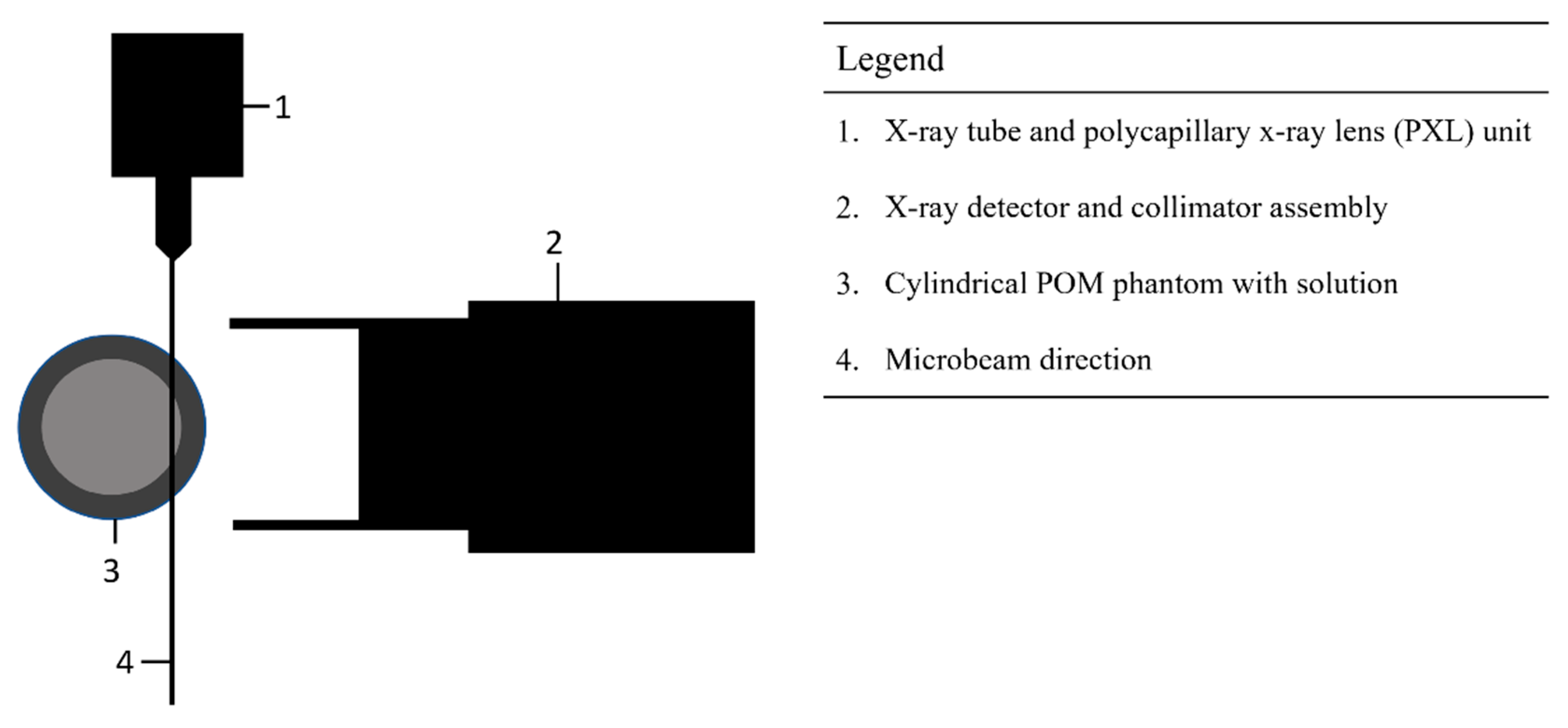
Figure 2.
Digital photograph of the 1.0-mm wall POM cylindrical cup suspended from the 3D-printed white plastic support attached to the positioning stage assembly (bottom of the image). The plastic support and cup assembly is placed in the center of the detector’s Al collimator (center-right part of the photo).
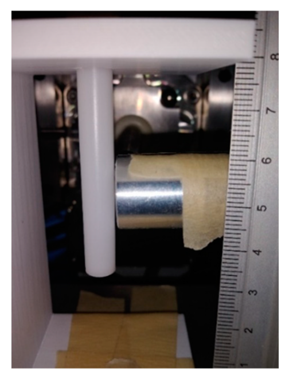
Figure 3.
Sample of function (red line) fitted to experimental data (black squares) obtained from the implementation of the experimental OGIP method. The insert table provided the corresponding values of all fitted parameters and their uncertainties.
Figure 3.
Sample of function (red line) fitted to experimental data (black squares) obtained from the implementation of the experimental OGIP method. The insert table provided the corresponding values of all fitted parameters and their uncertainties.
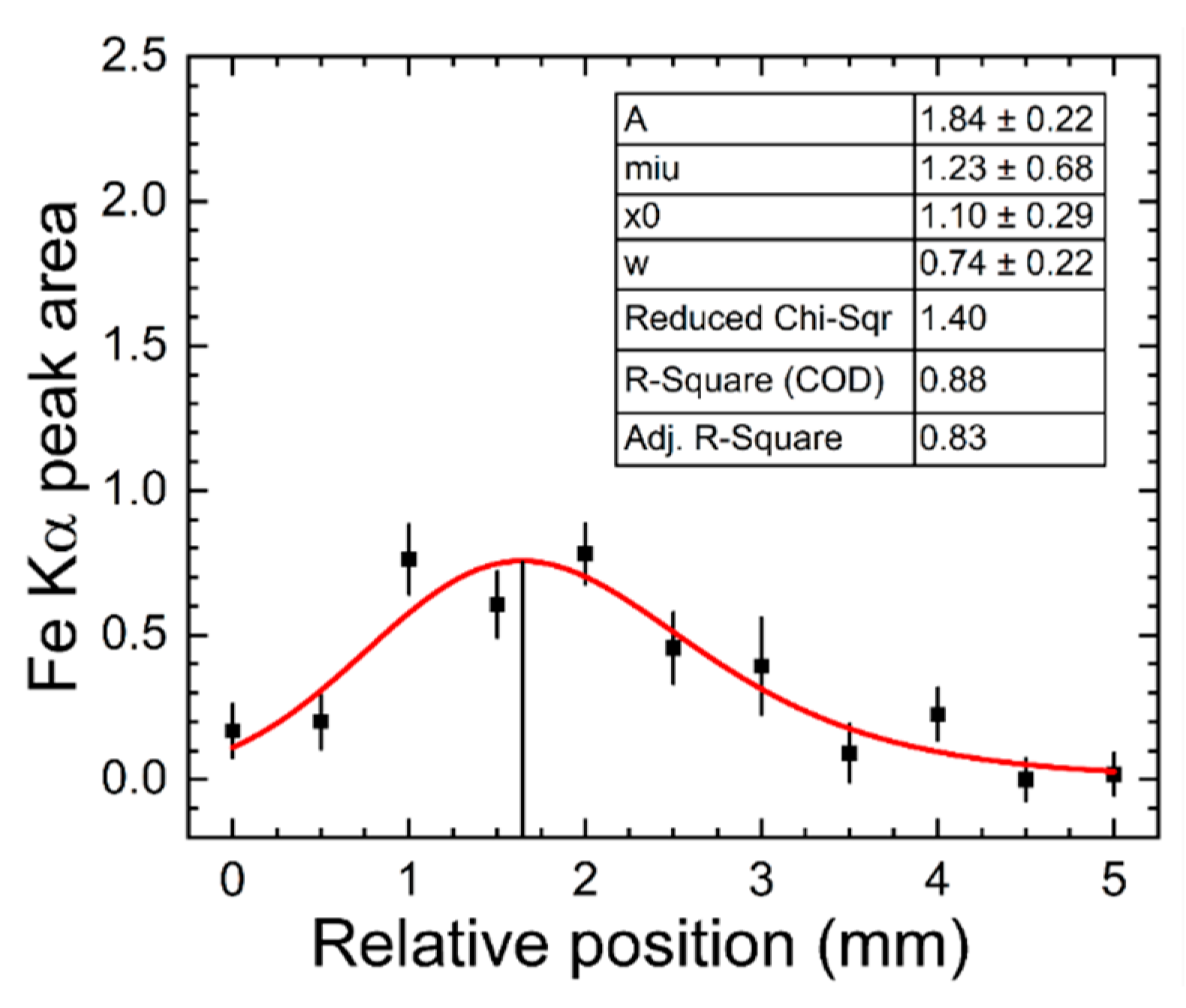
Figure 4.
Sample plots of the entire x-ray spectrum (left) and nonlinear fitting results for the five photon energy intervals marked by continuous curves of different colors (right). Data corresponds to solution 5 and 0.6 mm POM cup with insert phantom configuration.
Figure 4.
Sample plots of the entire x-ray spectrum (left) and nonlinear fitting results for the five photon energy intervals marked by continuous curves of different colors (right). Data corresponds to solution 5 and 0.6 mm POM cup with insert phantom configuration.
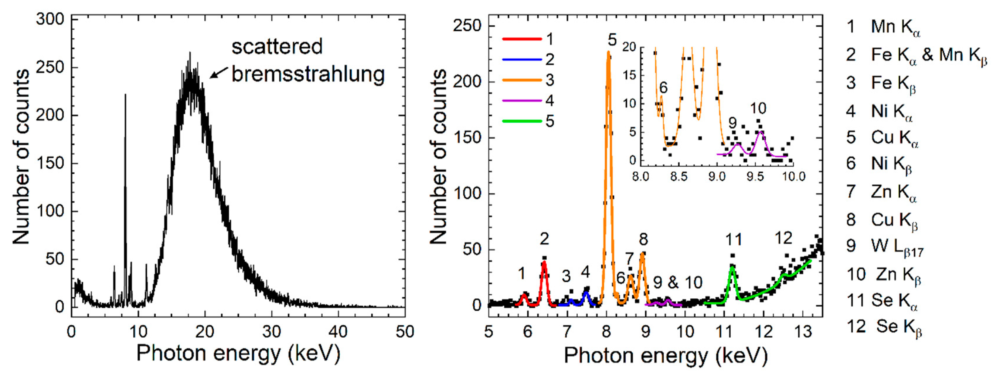
Figure 5.
Calibration lines of the measured Kα peak area of Fe and Zn in the three phantom configurations.
Figure 5.
Calibration lines of the measured Kα peak area of Fe and Zn in the three phantom configurations.
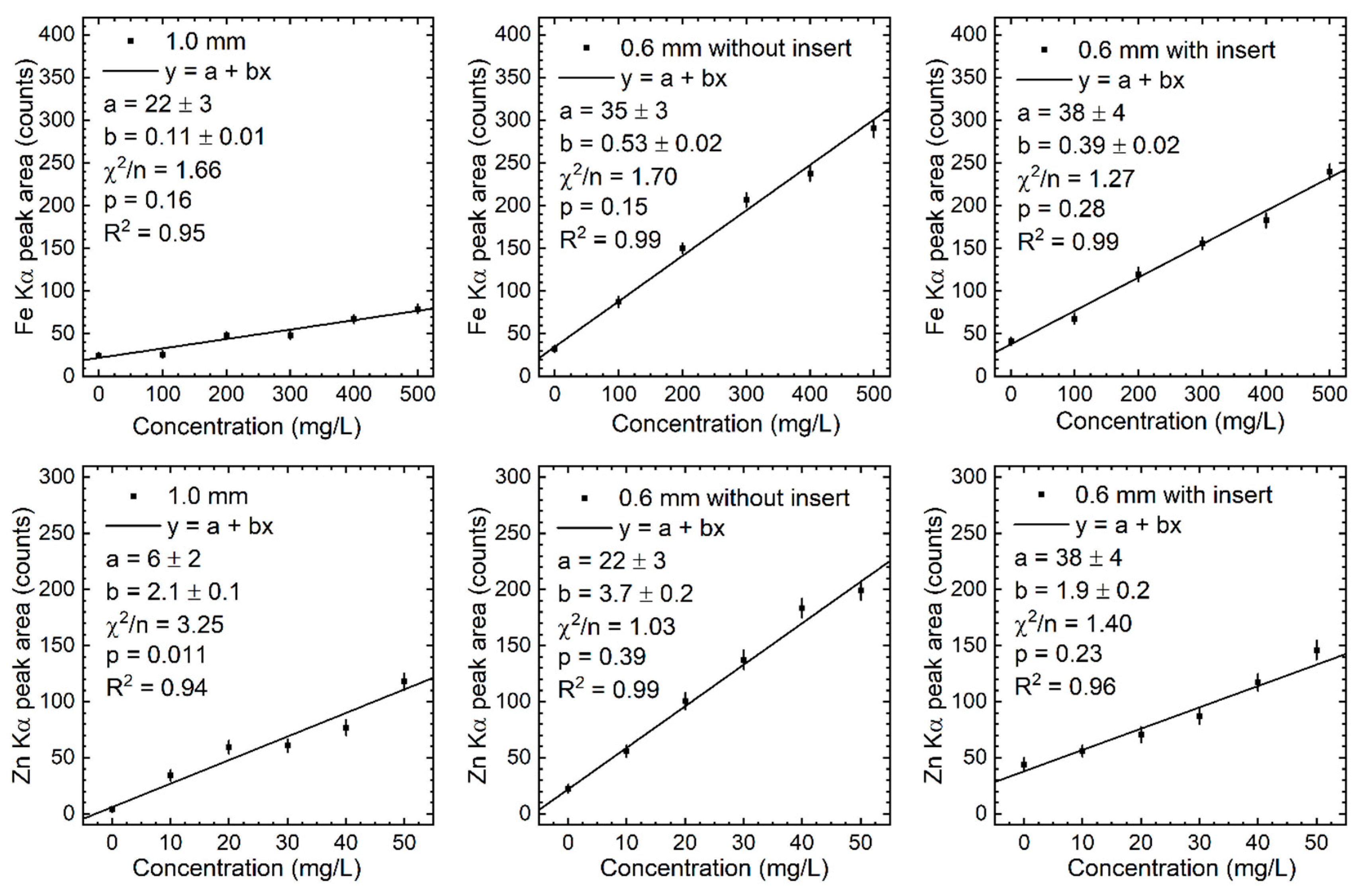
Figure 6.
Calibration lines of the measured Kα peak area of Cu and Se in the three phantom configurations.
Figure 6.
Calibration lines of the measured Kα peak area of Cu and Se in the three phantom configurations.
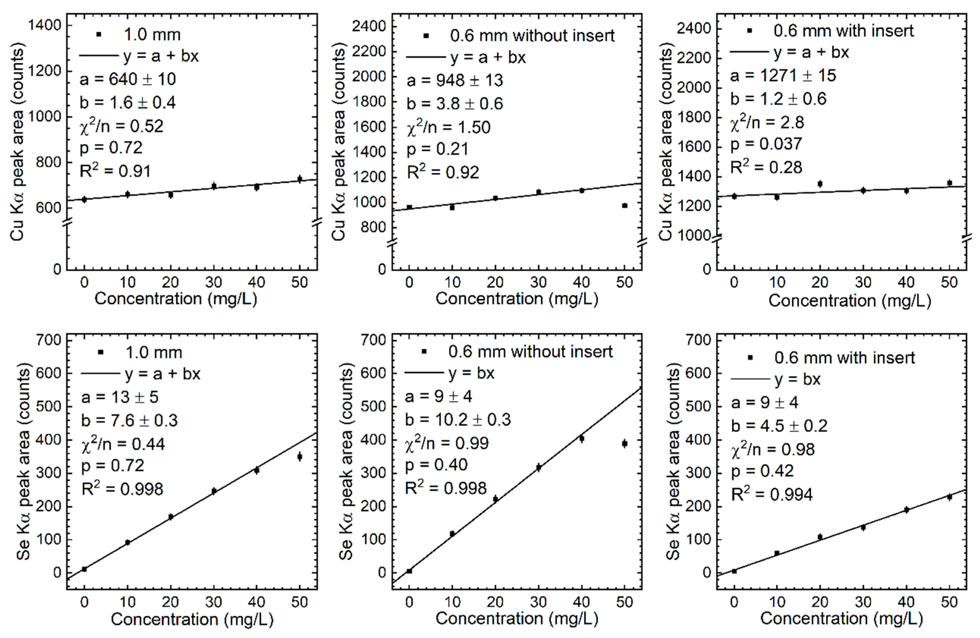
Figure 7.
Calibration lines of the measured Kβ peak area of Fe and Zn in the three phantom configurations.
Figure 7.
Calibration lines of the measured Kβ peak area of Fe and Zn in the three phantom configurations.
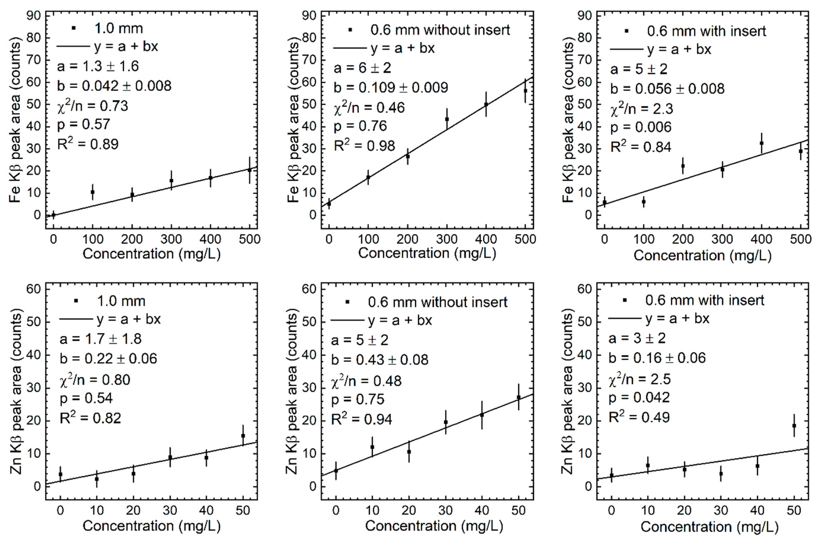
Figure 8.
Calibration lines of the measured Kβ peak area of Cu and Se in the three phantom configurations.
Figure 8.
Calibration lines of the measured Kβ peak area of Cu and Se in the three phantom configurations.
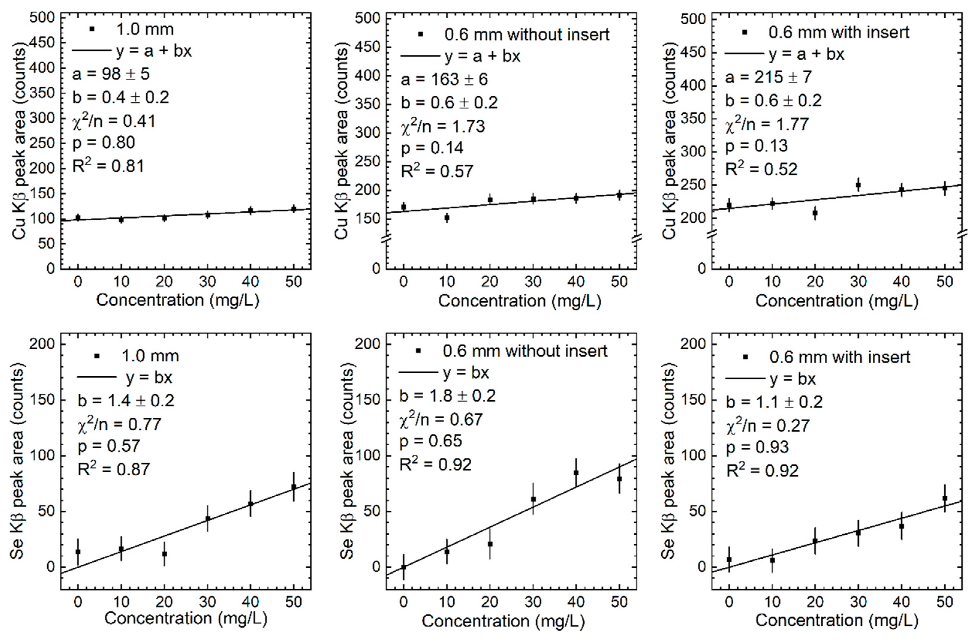

Table 1.
Table of Fe, Cu, Zn, and Se concentrations measured in human whole blood in mg/L units.
| Element | Z | Range | Arithmetic Mean | Geometric Mean | Median | Ref. | |
| Min | Max | ||||||
| Fe | 26 | 387 | 554 | 472 | 469 | 476 | [58] |
| 468 | 631 | 541 | [68] | ||||
| Cu | 29 | 0.610 | 1.900 | 0.920 | [69] | ||
| 0.720 | 1.800 | 1.042 | 1.020 | [59] | |||
| 0.776 | 1.495 | 1.036 | 1.011 | [60] | |||
| 0.720 | 1.020 | 0.875 | 0.870 | 0.873 | [58] | ||
| 0.580 | 1.590 | 0.795 | [62] | ||||
| 0.650 | 1.420 | 0.840 | [63] | ||||
| 0.676 | 1.837 | 1.078 | 1.040 | [70] | |||
| 0.820 | 1.270 | 1.010 | [68] | ||||
| Zn | 30 | 6.100 | 3.100 | 9.800 | [69] | ||
| 4.686 | 8.585 | 6.418 | 6.387 | [60] | |||
| 3.684 | 6.668 | 4.938 | 4.845 | 4.863 | [58] | ||
| 4.770 | 7.272 | 5.876 | 5.805 | 5.844 | [71] | ||
| 3.700 | 7.250 | 5.477 | [62] | ||||
| 4.620 | 9.250 | 6.750 | [63] | ||||
| 4.424 | 17.152 | 8.085 | 7.629 | [70] | |||
| 5.900 | 9.100 | 7.500 | [68] | ||||
| Se | 34 | 0.110 | 0.055 | 0.180 | [69] | ||
| 0.085 | 0.182 | 0.133 | 0.132 | [59] | |||
| 0.106 | 0.185 | 0.140 | 0.138 | [60] | |||
| 0.080 | 0.155 | 0.110 | [62] | ||||
| 0.118 | 0.224 | 0.141 | [63] | ||||
| 0.061 | 0.201 | 0.115 | 0.113 | [70] | |||
| 0.075 | 0.137 | 0.100 | [68] | ||||
Table 2.
List of the initial elemental concentrations, volumes, and calculated elemental masses for the four atomic absorption standard solutions.
Table 2.
List of the initial elemental concentrations, volumes, and calculated elemental masses for the four atomic absorption standard solutions.
| Element | Solvent c(HNO3) |
(mg/L) |
(mg/L) |
(mL) |
(mL) |
(mg) |
(mg) |
|---|---|---|---|---|---|---|---|
| Fe | 2% w/w | 1001 | 4 | 2 | 0.002 | 2.002 | 0.008 |
| Cu | 2% w/w | 1001 | 4 | 0.2 | 0.002 | 0.2002 | 0.0008 |
| Zn | 2% w/w | 1001 | 4 | 0.2 | 0.002 | 0.2002 | 0.0008 |
| Se | 0.5 mol/L | 1001 | 4 | 0.2 | 0.002 | 0.2002 | 0.0008 |
Table 3.
Elemental concentrations () and their uncertainties () for each of the five water-based solutions made from diluting the mixture of initial atomic absorption standard solution volumes provided in table 2.
Table 3.
Elemental concentrations () and their uncertainties () for each of the five water-based solutions made from diluting the mixture of initial atomic absorption standard solution volumes provided in table 2.
| Solution number | (mL) |
(mL) |
(mg/L) |
(mg/L) |
||||||
| Fe | Cu | Zn | Se | Fe | Cu | Zn | Se | |||
| 1 | 17.4 | 0.102 | 100 | 10 | 10 | 10 | 1 | 0.1 | 0.1 | 0.1 |
| 2 | 7.4 | 0.102 | 200 | 20 | 20 | 20 | 2 | 0.3 | 0.3 | 0.3 |
| 3 | 4.1 | 0.002 | 299 | 30 | 30 | 30 | 1 | 0.1 | 0.1 | 0.1 |
| 4 | 2.4 | 0.004 | 400 | 40 | 40 | 40 | 2 | 0.2 | 0.2 | 0.2 |
| 5 | 1.4 | 0.002 | 501 | 50 | 50 | 50 | 2 | 0.2 | 0.2 | 0.2 |
Table 4.
Sizes of the two POM cylindrical cups and solid cylindrical insert.
| POM sample |
Outer diameter (mm) |
Inner diameter (mm) |
Wall thickness (mm) |
Length (cm) |
| 1.0 mm wall cup | 7.5 | 5.5 | 1.0 | 5.0 |
| 0.6-mm wall cup | 7.5 | 6.3 | 0.6 | 5.0 |
| cylindrical insert | 5.3 | – | – | 4.9 |
Table 5.
X-ray linear attenuation coefficient () values at four different photon energies. See text for details.
Table 5.
X-ray linear attenuation coefficient () values at four different photon energies. See text for details.
| X-ray linear attenuation coefficient | (mm−1) | |||
| Photon energy (keV) | 5 | 10 | 15 | 20 |
| Water solution 5 (1.00 g/cm3) | 4.27 × 100 | 5.44 × 10⁻¹ | 1.71 × 10⁻¹ | 8.28 × 10⁻² |
| Human blood (1.06 g/cm3) | 4.49 × 100 | 5.85 × 10⁻¹ | 1.85 × 10⁻¹ | 8.93 × 10⁻² |
| POM (1.40 g/cm3) | 4.65 × 100 | 5.81 × 10⁻¹ | 1.86 × 10⁻¹ | 9.28 × 10⁻² |
| Human skin (1.09 g/cm3) | 4.56 × 100 | 5.39 × 10⁻¹ | 1.71 × 10⁻¹ | 8.37 × 10⁻² |
Table 6.
Observed XRF peaks fitted by each of the five peak fitting functions and their known or presumed origin.
Table 6.
Observed XRF peaks fitted by each of the five peak fitting functions and their known or presumed origin.
| No. | XRF peaks (Siegbahn nomenclature) |
Origin of observed XRF peaks | |
|---|---|---|---|
| 1 | 2 | Mn Kα, Fe Kα | solution & metallic parts of XRF system |
| 2 | 2 | Ni Kα, Fe Kβ | solution & metallic parts of XRF system |
| 3 | 4 | Cu Kα, Ni Kβ, Zn Kα, Cu Kβ | solution & metallic parts of XRF system |
| 4 | 2 | W Lβ17, Zn Kβ | solution & x-ray tube anode material |
| 5 | 2 | Se Kα, Se Kβ | solution |
Table 7.
Measured parameters and detection limit (DL) values for 1.0-mm wall cup phantom configuration.
Table 7.
Measured parameters and detection limit (DL) values for 1.0-mm wall cup phantom configuration.
| Peak | W. av. | |||||||||||
| Quantity | ||||||||||||
| Unit | counts mg−1 L | counts | mg/L | counts mg−1 L | counts | mg/L | mg/L | |||||
| Fe | 0.11 | 0.01 | 3.351 | 91 | 8 | 0.042 | 0.008 | 1.749 | 125 | 24 | 95 | 8 |
| Cu | 1.6 | 0.4 | 13.942 | 26 | 7 | 0.4 | 0.2 | 6.284 | 47 | 24 | 28 | 6 |
| Zn | 2.1 | 0.1 | 2.478 | 3.5 | 0.2 | 0.22 | 0.06 | 2.341 | 32 | 9 | 3.6 | 0.2 |
| Se | 7.6 | 0.3 | 5.413 | 2.14 | 0.08 | 0.035 | 0.004 | 0.299 | 26 | 3 | 2.2 | 0.1 |
Table 8.
Measured parameters and detection limit (DL) values for 0.6-mm wall cup without insert phantom configuration.
Table 8.
Measured parameters and detection limit (DL) values for 0.6-mm wall cup without insert phantom configuration.
| Peak | W. av. | |||||||||||
| Quantity | ||||||||||||
| Unit | counts mg−1 L | counts | mg/L | counts mg−1 L | counts | mg/L | mg/L | |||||
| Fe | 0.53 | 0.02 | 4.02471 | 22.8 | 0.9 | 0.109 | 0.009 | 2.300 | 63 | 5 | 24 | 1 |
| Cu | 3.80 | 0.6 | 16.494 | 13 | 2 | 0.6 | 0.2 | 7.730 | 39 | 13 | 14 | 2 |
| Zn | 3.7 | 0.2 | 3.805 | 3.1 | 0.2 | 0.43 | 0.08 | 2.697 | 19 | 4 | 3.1 | 0.2 |
| Se | 10.2 | 0.3 | 4.893 | 1.44 | 0.04 | 1.8 | 0.2 | 11.498 | 19 | 2 | 1.45 | 0.04 |
Table 9.
Measured parameters and detection limit (DL) values for 0.6-mm wall cup with insert phantom configuration.
Table 9.
Measured parameters and detection limit (DL) values for 0.6-mm wall cup with insert phantom configuration.
| Peak | W. av. | |||||||||||
| Quantity | ||||||||||||
| Unit | counts mg−1 L | counts | mg/L | counts mg−1 L | counts | mg/L | mg/L | |||||
| Fe | 0.39 | 0.02 | 4.583 | 35 | 2 | 0.056 | 0.008 | 2.339 | 125 | 18 | 36 | 2 |
| Cu | 1.2 | 0.6 | 20.176 | 50 | 25 | 0.6 | 0.2 | 9.322 | 47 | 16 | 48 | 13 |
| Zn | 1.9 | 0.2 | 5.973 | 9 | 1 | 0.16 | 0.06 | 2.113 | 40 | 15 | 10 | 1 |
| Se | 4.5 | 0.2 | 5.036 | 3.4 | 0.1 | 1.1 | 0.2 | 11.281 | 31 | 6 | 3.4 | 0.1 |
Table 10.
Detection limits for the three phantom configurations and reported human blood concentration ranges of the four elements as extracted from table 1. All values are in mg/L.
Table 10.
Detection limits for the three phantom configurations and reported human blood concentration ranges of the four elements as extracted from table 1. All values are in mg/L.
| Element | 1.0 mm wall cup | 0.6 mm wall cup without insert | 0.6 mm wall cup with insert | Human blood concentration range |
| Fe | 95 8 | 24 1 | 36 2 | 387 – 631 |
| Cu | 28 6 | 14 2 | 48 13 | 0.580– 0.90 |
| Zn | 3.6 0.2 | 3.1 0.2 | 10 1 | 3.684 – 17.152 |
| Se | 2.2 0.1 | 1.45 0.04 | 3.4 0.1 | 0.055 – 0.224 |
Table 11.
Physical parameters and dose rate values for the three phantom configurations. The absorbed dose values in the last column correspond to a single 180-s x-ray exposure.
Table 11.
Physical parameters and dose rate values for the three phantom configurations. The absorbed dose values in the last column correspond to a single 180-s x-ray exposure.
| Phantom configuration | (mm) | (mm) | (g) | (g) | (keV) | Dose rate (mGy/s) | Dose (mGy) |
| 1 mm POM | 5.50 | 1.00 | 0.012 | 0.006 | 8.669 | 0.26 | 47 |
| 0.6 mm POM without insert | 6.30 | 0.60 | 0.014 | 0.004 | 8.545 | 0.27 | 48 |
| 0.6 mm POM with insert | 1.00 | 3.25 | 0.002 | 0.021 | 9.350 | 0.23 | 42 |
Table 12.
Numerical values for , , and ratios. Numbers in the round parentheses are the uncertainties in the last significant figure. See text for additional details.
Table 12.
Numerical values for , , and ratios. Numbers in the round parentheses are the uncertainties in the last significant figure. See text for additional details.
| Phantom configuration | ||||||
| Fe | Cu | |||||
| 1.0 mm cup | 0.44(9) | 0.132(5) | 3.4(7) | 0.3(1) | 0.136(3) | 1.8(9) |
| 0.6 mm cup w/o insert | 0.20(2) | 1.5(1) | 0.15((5) | 1.1(4) | ||
| 0.6 mm cup with insert | 0.15(2) | 1.1(2) | 0.4(2) | 3(1) | ||
| Zn | Se | |||||
| 1.0 mm cup | 0.13(2) | 0.138(5) | 0.9(2) | 0.19(2) | 0.161(5) | 1.2(2) |
| 0.6 mm cup w/o insert | 0.11(2) | 0.8(2) | 0.19(2) | 1.2(1) | ||
| 0.6 mm cup with insert | 0.4(2) | 0.6(3) | 0.26(4) | 1.6(2) | ||
Disclaimer/Publisher’s Note: The statements, opinions and data contained in all publications are solely those of the individual author(s) and contributor(s) and not of MDPI and/or the editor(s). MDPI and/or the editor(s) disclaim responsibility for any injury to people or property resulting from any ideas, methods, instructions or products referred to in the content. |
© 2025 by the authors. Licensee MDPI, Basel, Switzerland. This article is an open access article distributed under the terms and conditions of the Creative Commons Attribution (CC BY) license (https://creativecommons.org/licenses/by/4.0/).
Copyright: This open access article is published under a Creative Commons CC BY 4.0 license, which permit the free download, distribution, and reuse, provided that the author and preprint are cited in any reuse.


