
Submitted:
24 February 2025
Posted:
25 February 2025
You are already at the latest version
Abstract
The study examines impacts of climate change on operation and capacity of the combined sewer network in the historic center of Thessaloniki, Greece. Rainfall data from three high-resolution Regional Climate Models (RCMs) from MED-CORDEX initiative with future estimations based on Representative Concentration Pathway (RCP) 4.5, are first corrected for bias based on existing measurements in the study area. Intensity-duration-frequency (IDF) curves are then constructed for the future data, using a temporal downscaling approach based on the scaling of the Generalized Extreme Value (GEV) distribution to derive the relationships between daily and sub-daily precipitation. Projected rainfall events associated with various return periods are subsequently developed and utilized as input parameters for the hydrologic-hydraulic model. The simulation results for each return period are compared with those of the current climate, and the projections from various RCMs are ranked according to their impact on the combined sewer network and overflow volumes.
Keywords:
Combined Sewer Overflows
; Regional Climate Models
; Temporal Downscaling
; intensity-duration-frequency curves
1. Introduction
A number of latest studies conducted by the Intergovernmental Panel on Climate Change (IPCC, 2014) reported evidence for changes in the occurrence of certain meteorological events during the 21st century. Regarding precipitation extremes in Europe, increased precipitation intensity in a future climate was one of the model results of most recent studies [1,2,3,4,5,6]. The IPCC assessments relied heavily upon the use of Global Circulation Models (GCMs), namely large mechanistic models for the global atmosphere, which are indeed coupled atmosphere-ocean models. Regional Climate Models (RCMs) are forced by the output of the GCMs as initial or boundary conditions and simulate regional climate with a finer resolution, enhancing the spatial resolution of climatic projections. During the previous years, different RCMs have been used to produce high-resolution climate scenario calculations on the European scale (e.g EU-projects PRUDENCE, ENSEMBLES and CORDEX), including the entire Mediterranean basin [7,8,9].
Future climate projections produced by climate models (GCMs and RCMs) are still subject to large uncertainties possibly originated from three major sources such as the emission uncertainty, the model uncertainty reflecting the limited understanding of the different atmospheric processes and their representation in the climatic models, as well as the uncertainty due to natural variability [10]. Especially when using RCM data, the drivers of uncertainty increase, as the model resolution, the forcing lateral conditions and physical parameterizations [11,12] induce more bias and variance in the results. Therefore, the aforementioned uncertainty sources should be considered when assessing the impacts of climate change on different domains, for the estimation process to be more reliable and robust. Model uncertainty can be considered by creating a multi-model ensemble, consisting of climate models that are ideally structurally independent. Kendon et al. [13] combined climate models through a multi-model ensemble to produce more reliable and consistent climate projections, suggesting the use of minimum three components to estimate changes in precipitation extremes.
Different scales (spatial and temporal) between RCMs and local measuring gauges or local urban drainage systems can have significant effects and produce inaccuracies on the precipitation process or the different sewer processes [14,15]. The aforementioned arguments may necessitate the use of dynamic or statistical downscaling methods to reduce the effects of the coarse scales of climate models to precipitation and urban drainage studies. Statistical downscaling includes methods that are quite easy to apply, are not time consuming and are considered rather efficient. This category of methods includes statistical models to transfer the “predictor” variables, which are available on a coarse grid, to the “predictand” variable, corresponding to finer spatial scales. Statistical downscaling methods include the construction of empirical transfer functions, weather typing models or stochastic modelling methods [16]. The former methods create and utilize transfer functions between the coarse scale variable of the climatic model and the smaller scale variable. Bias correction methods include the development of transfer functions between the cumulative distribution functions of the climate model and observed data. Bias represents the error component of the climate model that is independent of time [17]. Among the bias correction techniques, recent studies mainly using precipitation and temperature data, indicated the quantile mapping methods as the most efficient, even for the most extreme part of the distribution of the studied variables [18,19,20,21]. Gudmundsson et al. [22] reviewed and classified bias correction methods using observations of a large number of precipitation stations in Norway achieving to systematically reduce biases in RCM precipitation projections. Teutschbein and Seibert [23] reviewed and evaluated different bias correction methods for hydrological climate change impact studies. Tani and Gobiet [20] developed an extended version of the quantile mapping approach to provide more reliable bias-corrected precipitation extremes by combining the advantages of nonparametric methods and extreme value theory. Chandra and Papalexiou [24] introduced a semi-parametric approach for correcting daily precipitation for bias, providing good results for extreme quantiles. Holthuijzen et al. [21] proposed a hybrid bias-correction method for precipitation, including a robust linear correction for extremes.
Another significant issue that should be considered refers to the fact that hydro-meteorological variables, such as precipitation, resulting from climate models, are not in general available in time series with fine temporal resolution (e.g., 10 min to 1 h time steps). However, these time scales are essential for studying and estimating the effects of climate change especially on medium or small catchment areas. Temporal downscaling and temporal disaggregation are used to overcome such a difficulty. Temporal downscaling usually refers to the generation of data of high temporal resolution by means of statistical techniques, most commonly stochastic models, calibrated using information on the statics of data from lower resolution temporal scales. The most commonly used downscaling approaches are statistical downscaling methods. Nguyen et al. [25] proposed a statistical temporal downscaling method which is based on the scaling Generalized Extreme Value (GEV) distribution to describe the relationships between daily and subdaily extreme precipitation. Terti et al. [26] evaluated the suitability of the abovementioned approach for determining the distribution of short-duration extreme rainfall in Thessaloniki, Greece. Ghanmi et al. [27] used the simple scale invariance concept to statistically downscale daily rainfall in northern Tunisia to subdaily amounts. Yeo et al. [28] used GEV scaling to estimate subdaily annual maximum precipitation from daily values and applied their methodology to available data from Quebec, Canada and Seoul, South Korea. Galiatsatou and Iliadis [29] applied a simple scaling approach based on the GEV distribution to assess short-duration rainfall extremes at ungauged sites transferring information from gauged ones with a relatively homogeneous extreme rainfall climate. Iliadis et al. [30] used a GEV scaling approach to daily rainfall extremes assessed from a long time series, to estimate fine temporal scale extreme events in Thessaloniki, Greece.
Intensity-Duration-Frequency (IDF) curves based on local precipitation measurements are currently utilized for engineering design and management applications, such as flood risk protection structures and infrastructures or flood mitigation projects. The IDF curves are constructed for different return periods representing the variation of rainfall intensity with duration. Theoretical probability distribution functions are fitted to annual maximum rainfall intensities of particular durations ranging from shorter ones e.g., 5 min to daily precipitation events. These curves are currently designed under the assumption of stationarity [31,32,33], namely the hypothesis that the occurrence probability of precipitation events will remain unaltered or will not exhibit significant changes in time, mainly due to the lack of predictability on details of possible future changes. But the fact is that such hydro-meteorological signals, especially at their extreme levels, exhibit phenomena of nonstationarity. Natural climatic variability, human interventions in the hydrologic cycle of different catchments areas and climate change are some of the prominent causes of such nonstationarities [34,35]. Yan et al. [36] reviewed literature on updating IDF curves under climate change, mainly emphasizing on covariate-based distributions for modelling extremes. Martel et al. [37] studied changes in extreme precipitation and related sources of uncertainty. Schlef et al. [38] presented a review on current knowledge and research on nonstationary IDF curves. Nonstationary IDF curves are usually constructed under the assumption of covariate-based modelling or simulated precipitation from RCMs or GCMs. In the latter case, precipitation extremes are obtained over historical and future periods (projections) from a number of climate models (RCMs or GCMs). However, there is currently an ongoing discussion on whether and to what degree nonstationarity should be addressed in design for hydroclimatic extremes, mainly focusing on uncertainty, model complexity, and data limitation issues [39,40].
Considering that there is an increasing evidence of climate change associated with destructive extreme events of higher intensity and frequency, combined with the deterioration process of the sewer network and the rapid growth of cities, an increase is expected in the number of people and properties in urban areas affected by the harmful effects of urban stormwater. In this context, urban drainage infrastructures are unlikely to be adequate in the future in the majority of cities worldwide, because their design relied upon the historical precipitation data ignoring the climatic variability. Kourtis and Tsihrintzis [41] reviewed the state-of-the-art of scientific approaches for adaptation of urban drainage networks to climate change, discussing climate change impacts on precipitation, IDF curves, flooding and urban drainage, and defined a novel approach for assessing urban drainage network adaptation to climate change and other drivers. Galiatsatou and Iliadis [29] introduced a methodological framework for designing urban drainage networks under climate change conditions, considering nonstationarity of the extreme precipitation in the study area. Galiatsatou et al. [42] conducted capacity assessment of a combined sewer network under the impact of rainfall storm events of different return periods, and proposed mitigation strategies, such as the application of nature-based solutions (NBSs) or low-impact developments (LIDs) for controlling combined sewer overflows. In this framework, the effects of climate change on the performance and capacity of the combined sewer system in Thessaloniki’s historic center, Greece.
2. Materials and Methods
2.1. Study Area
This study focuses on the historic center of Thessaloniki, a city in northern Greece. Thessaloniki is the country’s second-largest city, with a population exceeding one million and a particularly high population density in the city center, estimated at 200 residents per hectare. The city’s annual average rainfall was recorded at 445.7 mm for the period 1960–2020, based on monthly data from the Hellenic National Meteorological Service (HNMS). During this period, the average monthly rainfall varied from a low of 21.1 mm in August to a peak of 54.5 mm in December. The study area is defined by Aristotelous Street to the west and Aggelaki Street to the east, with its northern boundary along Egnatia and Svolou streets, and its southern boundary along Leoforos Nikis on the city’s coastal front. The selected area, covering approximately 40 hectares, along with the layout of Thessaloniki’s examined sewer network, is presented in Figure 1.
2.2. Climate Data Assessment and Downscaling Methodology
Historical precipitation measurements were obtained from the Meteorological Station (MS) of the Aristotle University of Thessaloniki (AUTH) which is located near the study area. These historical records covered the period from October 1965 to September 2005. The AUTH station has been widely recognized for its long-term, high-quality data collection, making it a reliable source for climatological analysis and model evaluation.
Future precipitation projections used in this study were sourced from the EURO-CORDEX Coordinated Downscaling Experiment [43], an initiative under the CORDEX framework. This dataset provides high-resolution regional climate simulations, ensuring the robustness of climate projections across Europe. For this analysis, monthly precipitation projections were derived from three distinct Regional Climate Models (RCMs) as presented in Table 1.
Each RCM provides a spatial resolution of 0.11o (approximately 12.5 km), offering a fine spatial grid suitable for local-scale climate impact studies. The future projections cover the period from October 2020 to September 2100 and were performed under the Representative Concentration Pathway (RCP) 4.5 scenario. This scenario represents an intermediate greenhouse gas emission pathway, where emissions peak around mid-century and then stabilize.
To ensure consistency and comparability, historical precipitation observations (1965–2005) were directly compared to the corresponding historical simulation outputs from the RCMs for the same period. Given the inherent biases present in raw precipitation outputs from RCMs, bias correction was necessary. The Bias Correction Quantile Mapping (BCQM) method was employed for this purpose, utilizing the qmap package [22] in R. This statistical technique adjusts the cumulative distribution of modeled precipitation to align with that of observed precipitation, thereby addressing systematic discrepancies. The BCQM approach uses a non-linear transformation to model the quantile–quantile relationship between observed and simulated precipitation values. Specifically, the exponential tendency to an asymptote transformation function was applied, as described by Gudmundsson et. al. [22]:
where is the observed variable, Xm is the modelled variable, and a,b,x and τ are parameters.
The bias-corrected transformation function was subsequently applied to the future climatic projections to adjust for biases in the raw outputs of the climate models. To enable a more detailed analysis of future climatic trends, the projected period spanning from 2010 to 2100 was divided into two distinct 40-year intervals: 2020-2060, representing the short-term projection, and 2060-2100, representing the long-term projection. The mean annual precipitation and its associated standard deviation were computed for both the historical period and the future time intervals for each of the three climate models after bias correction.
2.3. The Scaling GEV Model
The GEV distribution has been used in several scientific studies for modelling annual series of extreme rainfall, as it has been proven that it matches well the observed extreme values. The cumulative distribution function (CDF), G(x), for the GEV distribution is given as:
where μ, σ and ξ are respectively the location, scale and shape parameters, the latter also determining its limiting behaviour. When the shape parameter, ξ, is equal to zero the GEV distribution is equivalent to the Gumbel distribution, while when ξ is higher or lower than zero, the GEV corresponds to the Fréchet and the (reversed) Weibull distribution families, respectively. In this work, due to the small sample size of the annual maximum rainfall series (40-year maxima for all study periods and climate models) the three parameters are estimated by the method of L-moments [44,45]. For the random variable X with distribution function F, the theoretical L-moments λr+1 with r=0, 1,.. are expressed as linear functions of the specific probability weighted moments (PWM):
with the dimensionless L-moment ratios L-skewness, τ3=λ3/λ2, and L-kurtosis, τ4=λ4/λ2, calculated as functions of the L-scale, λ2, and the third, λ3, and fourth, λ4, L-moments. Let ar be the unbiased estimator of ar for an ordered sample x1:n≤…≤xn:n [45]:
with the unbiased sample L-skewness, t3=l3/l2, and L-kurtosis, t4=l4/l2, calculated as functions of the sample L-scale, l2, and the third, l3, and fourth, l4, sample L-moments, respectively. If the L-moments estimation method results in a quite low estimate of the shape parameter (estimate close to -0.5) of the extreme precipitation process for a certain time interval and climate realization scenario, the maximum likelihood estimation (MLE) procedure is also applied to estimate the GEV parameters [46,47].
After the parameters’ estimation, the quantiles XΤ for each return period T can be calculated as follows:
It can be shown that the k-th order of Non-Central Moments (NCM), mk, can be expressed as a function of the three GEV parameters as:
For k=1, 2, 3 equation (5) can be written as follows:
where Γ(.) is the gamma function. In this work, the temporal downscaling method proposed by Nguyen et al. [25] and based on the “scale-invariance” concept, is utilized to statistically downscale daily rainfall hindcasts and predictions into finer temporal scales to assist the construction of IDF/DDF curves under different climate realizations. By definition, a function is scaling (or scale-invariant) if f(x) is proportional to the scaled function f(λx) for all positive values of the scale factor λ. Then, there exists a function C(λ) such that:
Nguyen et al. [25] proved that:
in which β is the scaling parameter and is considered constant. Therefore, the relationship between the NCM of order k, mk, and the variable x, can be expressed as [48]:
in which:
If equation (9) is log-transformed the NCM of order k can be written as:
Therefore, the three GEV parameters for subdaily rainfall annual maxima can be assessed from the respective annual maximum daily GEV parameters. More specifically, the GEV parameters for the two different time scales t and λt (λ≤1) are assessed as follows: the shape parameters of durations t and λt are assumed equal, and the location and scale parameters of durations t and λt are related by λβ. In the present work, a more elaborate approach is used. The shape parameter of the process, ξ, is assumed to change with duration and not to remain constant, in order to achieve better accuracy of the method. Precipitation can present different scaling regimes, therefore during distinct time intervals, the process can present different scaling parameters, β. Therefore, if a process is characterized by scaling regimes in the intervals [t1, t2] and [t2, t3], then it can be described as:
After assessing the GEV parameters of finer temporal scales from daily rainfall, IDF and DDF curves can be fully defined for all time periods and climate realizations considered. The general IDF and DDF relationship used in this work, considering that dependence in rainfall duration, d, and return period, T, can be modelled separately is:
where K, b, and c are coefficients to be determined by the available data for each period of interest.
2.4. Hydrologic and Hydraulic Model Configuration
In this study, the InfoWorks ICM (Integrated Catchment Modelling) software was selected to evaluate and assess the drainage system within the study area [49]. Developed by Innovyze, InfoWorks ICM is an advanced tool designed for managing combined sewer and stormwater systems. It facilitates detailed hydrologic and hydraulic modeling, enabling the analysis of sewer networks, assessment of existing infrastructure capacity, and planning of network upgrades. The software has been extensively applied in urban catchment modeling, as well as in studies related to urban flood hazards and flood risk assessment [50,51,52,53,54,55]. InfoWorks ICM supports integrated 1D and 2D hydrological and hydraulic simulations. To model surface flow, the nonlinear shallow water equations were employed, while the continuity and momentum equations were solved using a finite volume scheme with a Riemann solver.
Detailed and comprehensive data on the sewer system within the study area were obtained from the Geographic Information System (GIS) database of Thessaloniki’s Water Supply and Sewerage Company S.A. (EYATH S.A.). The collected data included analytical information on system links (conduits), such as their lengths (m), diameters (mm), and materials, as well as details regarding system nodes (e.g., inlets, manholes), including ground and invert elevations (m). Shapefiles containing all network elements were imported into InfoWorks ICM using the software’s open data import center. Additionally, IDF (Intensity-Duration-Frequency) curves were developed based on historical rainfall events and data from the Regional Climate Models: CCLM, RACMO, and REMO. Rainfall amounts corresponding to return periods of 2, 10, 50, and 100 years with a duration of 1 hour were initially determined. Subsequently, these total rainfall amounts were distributed over the duration of the storm event using the alternating block method.
3. Results
3.1. Projected Outcomes of Climate Models
The results, presented in Table 2, Table 3 and Table 4, illustrate the variability and potential shifts in precipitation dynamics at different temporal scales, highlighting inter-model differences and uncertainties inherent in future projections, and emphasizing the necessity of incorporating variability and uncertainty considerations into climate adaptation strategies.
The analysis of annual maximum daily precipitation reveals significant variability in its temporal distribution across the three climate models, as shown in Figure 2. These variations highlight the distinct responses of each climate model to the projected climatic conditions under the RCP4.5 scenario.
For the historical period (1965–2005), the average annual maximum daily precipitation was estimated at 41.04 mm/day, serving as the baseline for comparison. Projections for the short-term future period (2020–2060) indicate that the average annual maximum daily precipitation is expected to decrease to 38.71 mm/day (a reduction of -5.68%) according to the CCLM4-8-17.v1 - CLMcom.ICHEC-EC-EARTH model. In contrast, an increase to 50.61 mm/day (a rise of +23.32%) is projected by the RACMO22E.v1 - KNMI.ICHEC-EC-EARTH model, while the REMO2009.v1 - MPI-CSC.MPI-M-MPI-ESM-LR model forecasts a decline to 37.33 mm/day (a reduction of -9.04%).
In the long-term future period (2060–2100), the projected trends exhibit also notable differences among the models. The CCLM4-8-17.v1 - CLMcom.ICHEC-EC-EARTH model projects a substantial increase in the average annual maximum daily precipitation to 52.95 mm/day, representing a +29.02% change relative to the historical baseline. Similarly, the RACMO22E.v1 - KNMI.ICHEC-EC-EARTH model predicts an elevated value of 48.16 mm/day, corresponding to a +17.35% increase. Conversely, the REMO2009.v1 - MPI-CSC.MPI-M-MPI-ESM-LR model estimates a moderate increase to 39.02 mm/day, equating to a -4.92% change compared to the historical period.
Furthermore, as illustrated in Figure 2, the annual maximum daily precipitation consistently exhibits average values that are higher than their respective medians. This characteristic underscore the right-skewness of the precipitation dataset, a statistical trait that reflects the occurrence of infrequent but intense precipitation events that significantly influence the mean. Right-skewed distributions are a well-documented feature of precipitation datasets, particularly in regions subject to pronounced seasonal variability or periodic extreme weather phenomena. This skewness is indicative of a climate regime where extreme events dominate precipitation trends, and it has important implications for hydrological modeling and risk assessment.
Further analysis of the box plots presented in Figure 2 reveals notable differences between the historical and future periods. Specifically, the whiskers of the box plots for the future periods (2020–2060 and 2060–2100) concerning the CCLM4-8-17.v1 - CLMcom.ICHEC-EC-EARTH model are significantly longer than those observed for the historical baseline (1965–2005). This observation suggests a wider range of variability in annual maximum daily precipitation in the future, indicating the potential for more extreme values. The lengthened whiskers in the future projections highlight the increased likelihood of extremely high values, emphasizing the importance of accounting for climate extremes in future planning scenarios. This is particularly relevant for infrastructure design, and flood risk assessment, where planning for variability and uncertainty is critical.
3.2. Development of IDF Curves
The scaling behaviour of rainfall extremes in the study area is assessed using available annual maximum rainfall data at the Thessaloniki airport (station Mikra) provided by the HNMS covering a period of 25 years (1963-1987), corresponding to durations of 5min, 10min, 15min, 30min, 1h, 2h, 3h, 6h, 12h, and 24h. L-moments approach is initially used to assess the GEV parameters for all rainfall durations of the available fine scale dataset. Equation (6) is then used to assess the three NCMs for all rainfall durations and a logarithmic plot of the first three NCMs of rainfall at Thessaloniki station with rainfall duration is then constructed (Figure 3). Figure 3 also includes the power laws (Eq.9) resulting for all three NCMs.
The log-linearity of the GEV NCMs of annual maximum rainfall is illustrated in the plot, indicating the power law dependency (i.e., scaling) of the statistical moments with duration (Eqs. 9 and 11). The slopes in the plot are proportional to the scaling exponent β. Two different scaling regimes are evident from Figure 1, one in the interval 5min to 30min and one in 30min to 24h, indicating a difference in extreme rainfall dynamic at the finest temporal scales. This difference is confirmed from linearity of the scaling exponent β(k) with moment order, k, shown in Figure 4(a, b) for the intervals of [5,30] min and [0.5, 24] h.
After assessing the relationships of GEV NCMs with extreme rainfall duration, the three NCMs of the daily rainfall predictions are used combined with the scaling exponent β(k), which is kept constant for all time intervals and climate realizations, to assess the coefficients a(k) (see Eq. 9) of the annual maximum precipitation process. These coefficients can be used to determine the newly defined NCMs mk for each subdaily rainfall duration (using Eq. 9). The three GEV NCMs for each rainfall duration are then utilized to assess the respective GEV parameters by means of Eq. (6). After assessing the GEV parameters for all rainfall durations and for all 40-year intervals considered, the extreme quantiles (return levels) corresponding to return periods of 2, 5, 10, 20, 50, 100, 200, 500 and 1000 years are estimated using Eq. (4). IDF and DDF curves are then created for all 40-year periods considered (historical and future periods from RCMs) based on Eq. (13). Figure 5 presents IDF and DDF curves in Thessaloniki, Greece for the historical/reference climate period (1965-2005). Figure 6 presents IDF curves for all climate models considered in this work (CCLM, RACMO, REMO) and for both future periods 2020-2060 and 2060-2100.
Table 5 presents IDF and DDF curve equations (Eq. 13) for the historical/reference climate period (1965-2005), as well as for the two future periods (2020-2060 and 2060-2100) for all three RCMs studied in this work.
Rainfall extremes for the future period 2020-2060 are assessed higher than those of the historical climate only for RACMO RCM. More specifically 100-year rainfall events of 1h duration are almost 39% higher than those of the historical climate. CCLM and REMO RCMs produce lower 100-year rainfall extremes (1 h duration) up to 17.3% and 20%, respectively. The future period 2060-2100 appears more energetic with respect to extreme precipitation events, compared to the future period 2020-2060. In the future period 2060-2100, 100-year rainfall events of 1 h duration are almost 150%, 7%, and 51.5% higher than those of the future period 2020-2060 for CCLM, RACMO and REMO RCM, respectively.
3.3. Hydraulic Results
The rainfall storm events used in this study were derived from the IDF curves developed in Section 3.2, which were constructed using advanced statistical methods and techniques. These IDF curves were specifically designed for Thessaloniki’s city center. Total rainfall amounts corresponding to return periods of 2, 10, 50, and 100 years with a duration of 1 hour were utilized. The model that was calibrated and validated in Galiatsatou et al. [42] is also employed in this study.
Figure 7 illustrates the hydraulic results for current conditions under the worst-case scenario of a 100-year return period storm event. Meanwhile, Figure 8, Figure 9 and Figure 10 show the results derived from rainfall distributions based on the CCLM, RACMO, and REMO climate models, respectively, for the periods 2020-2060 and 2060-2100. Flooding correlation is assessed by examining conduit surcharge conditions and the hydraulic grade line (HGL) at nodes relative to a predefined theoretical basement elevation of 2 meters below ground level. To simplify result visualization, the color-coded figures display only the HGL. Black dots represent manholes, while dark blue lines along the coastal front indicate CSO points in the network. Sewer segments are color-coded as follows: green when the HGL remains more than 2 meters below the surface, purple when basement flooding occurs (HGL is less than 2 meters from the surface but remains underground), and red when surface flow is present. For simplicity, results for events with a return period of less than 100 years are not presented, as the issue is more effectively highlighted under the worst-case scenario.
Table 6 provides a summary of the simulation results and the impact of future climate projections on combined sewer overflow volumes (CSO volumes).
As shown in Figure 7, Figure 8, Figure 9 and Figure 10 and Table 6, in the near-term period from 2020 to 2060, the projected CSO volumes vary significantly across the models. The CCLM (10,735 m³) and REMO (10,012 m³) models predict lower overflow volumes compared to the existing conditions (12,273 m³), suggesting that these models anticipate either a decrease in extreme rainfall intensity or a redistribution of rainfall events. However, the RACMO model (17,117 m³) shows an increase in CSO volumes, indicating a potential rise in extreme precipitation events under this scenario. For the long-term period from 2060 to 2100, all models predict an increase in CSO volumes compared to existing conditions, highlighting a worsening overflow problem in the future. Among them, CCLM (25,514 m³) projects the highest overflow volume, more than doubling the existing conditions. This suggests that under this scenario, intense rainfall events will become significantly more frequent or severe, putting additional stress on urban drainage systems. The RACMO model (18,605 m³) also indicates a continuous increase in CSO volumes, though at a lower magnitude than CCLM, while REMO (15,799 m³) suggests a moderate increase over time. These projections carry important implications for future flood management strategies. The substantial increase in overflow volumes predicted by the CCLM model indicates that the most robust adaptation measures may be necessary in this scenario. These could include significant infrastructure enhancements such as increasing storage capacity, upgrading conveyance systems, and implementing nature-based solutions like green infrastructure. The variations among the models highlight the uncertainty in climate projections, underscoring the need for adaptable and flexible flood management strategies capable of addressing a broad spectrum of potential future conditions.
4. Conclusions
This study emphasizes the substantial effects of climate change on combined sewer overflows, particularly within the Thessaloniki City Centre network. The analysis of current and future IDF curves, derived from climate models CCLM, RACMO, and REMO, indicates that the system will encounter significant challenges due to increasing rainfall intensity. Modeling with InfoWorks shows that the expected rise in rainfall intensity may exceed the system’s capacity to handle peak flows, potentially leading to flooding risks and higher overflow volumes. To mitigate these issues, strategies such as separating stormwater and sanitary flows, disconnecting downspouts, and implementing nature-based solutions should be considered. These measures would improve the system’s resilience, reduce flood risks, and support long-term urban sustainability in the face of climate change. Future research will focus on addressing capacity issues using offline storage and low-impact development techniques.
Author Contributions
Conceptualization, P.G., I.N., D.M. and P.G.; methodology, P.G., I.N. and D.M.; software, P.G., I.N., D.M., M.K. and A.G.; validation, P.G., I.N., D.M., A.G. and A.Z.; formal analysis, P.G., I.N. and D.M.; investigation, P.G., I.N., D.M., M.K., A.G., and A.K.; resources, P.G., I.N., D.M., A.K.; data curation, I.N., D.M. M.K., A.G., A.K., D.M. and P.G.; writing—original draft preparation, P.G., I.N., D.M., M.K. and A.G.; writing—review and editing, P.G., I.N., D.M., A.Z., A.G., M.K., A.K., and P.G.; visualization, P.G., I.N., M.K. and D.M.; supervision, P.G., I.N., D.M. and A.Z.; project administration, A.Z. All authors have read and agreed to the published version of the manuscript.
Funding
This research received no external funding.
Data Availability Statement
No new data was created.
Acknowledgments
The authors wish to thank EYATH S.A. for providing the necessary data of this research and Lithos Group Inc. for granting the InfoWorks ICM software license used in conducting the hydraulic simulations.
Conflicts of Interest
The authors declare no conflict of interest.
References
- Colmet-Daage, A., Sanchez-Gomez, E., Ricci, S., Llovel, C., Borrell Estupina, V., Quintana-Seguí, P., ...; Servat, E. Evaluation of uncertainties in mean and extreme precipitation under climate change for northwestern Mediterranean watersheds from high-resolution Med and Euro-CORDEX ensembles. Hydrology and Earth System Sciences 2018, 22, 673–687. [Google Scholar] [CrossRef]
- Tramblay, Y.; Somot, S. Future evolution of extreme precipitation in the Mediterranean. Climatic Change 2018, 151, 289–302. [Google Scholar] [CrossRef]
- Berg, P.; Christensen, O.B.; Klehmet, K.; Lenderink, G.; Olsson, J.; Teichmann, C.; Yang, W. Summertime precipitation extremes in a EURO-CORDEX 0.11∘ ensemble at an hourly resolution. Natural Hazards and Earth System Sciences 2019, 19, 957–971. [Google Scholar] [CrossRef]
- Cardell, M.F.; Amengual, A.; Romero, R.; Ramis, C. Future extremes of temperature and precipitation in Europe derived from a combination of dynamical and statistical approaches. International Journal of Climatology 2020, 40, 4800–4827. [Google Scholar] [CrossRef]
- Di Sante, F.; Coppola, E.; Giorgi, F. Projections of river floods in Europe using EURO-CORDEX, CMIP5 and CMIP6 simulations. International Journal of Climatology 2021, 41, 3203–3221. [Google Scholar] [CrossRef]
- Ivušić, S.; Güttler, I.; Horvath, K. Overview of mean and extreme precipitation climate changes across the Dinaric Alps in the latest EURO-CORDEX ensemble. Climate dynamics 2024, 1–31. [Google Scholar] [CrossRef]
- Vautard, R.; Kadygrov, N.; Iles, C.; Boberg, F.; Buonomo, E.; Bülow, K.; Coppola, E.; Corre, L.; van Meijgaard, E.; Nogherotto, R.; Sandstad, M.; Schwingshackl, C.; Somot, S.; Aalbers, E.; Christensen, O.; Ciarlo, J.; Demory, M.; Giorgi, F.; Jacob, D.; Jones, R.; Keuler, K.; Kjellström, E.; Lenderink, G.; Levavasseur, G.; Nikulin, G.; Sillmann, J.; Solidoro, C.; Sørland, S.; Steger, C.; Teichmann, C.; Warrach-Sagi, K.; Wulfmeyer, V. Evaluation of the Large EURO-CORDEX Regional Climate Model Ensemble. JGR Atmphosheres 2021, 126, e2019JD032344. [Google Scholar] [CrossRef]
- Boe, J.; Mass, A.; Deman, J. A simple hybrid statistical–dynamical downscaling method for emulating regional climate models over Western Europe. Evaluation, application, and role of added value? Clim Dyn 2022, 61, 271–294. [Google Scholar] [CrossRef]
- Ascenso, A.; Augusto, B.; Coelho, S.; Menezes, I.; Monteiro, A.; Rafael, S.; Ferreira, J.; Gama, C.; Roebeling, P.; Miranda, A.I. Assessing Climate Change Projections through High-Resolution Modelling: A Comparative Study of Three European Cities. Sustainability 2024, 16, 7276. [Google Scholar] [CrossRef]
- Cox, P.; Stephenson, D. Climate change - A changing climate for prediction. Science 2007, 317, 207–208. [Google Scholar] [CrossRef]
- Déqué, M.; Rowell, D.P.; Lüthi, D.; Giorgi, F.; Christensen, J.H.; Rockel, B.; Jacob, D.; Kjellström, E.; de Castro, M.; van den Hurk, B. An intercomparison of regional climate simulations for Europe: assessing uncertainties in model projections. Climatic Change 2007, 81, 53–70. [Google Scholar] [CrossRef]
- Elía, R.; Caya, D.; Côté, H.; Frigon, A.; Biner, S.; Giguère, M.; Paquin, D.; Harvey, R.; Plummer, D. Evaluation of uncertanties in the CRCM-simulated North American climate. Climate Dynamics 2008, 30, 113–132. [Google Scholar] [CrossRef]
- Kendon, E.J.; Rowell, D.P.; Jones, R.G.; Buonomo, E. Robustness of future changes in local precipitation extremes. Journal of Climate 2008, 21, 4280–4297. [Google Scholar] [CrossRef]
- Gogien, F.; Dechesne, M.; Martinerie, R.; Lipeme Kouyi, G. Assessing the impact of climate change on Combined Sewer Overflows based on small time step future rainfall timeseries and long-term continuous sewer network modelling. Water Research 2023, 230, 119504. [Google Scholar] [CrossRef] [PubMed]
- Zhang, H.; Yang, Z.; Cai, Y.; Qiu, J.; Huang, B. Impacts of Climate Change on Urban Drainage Systems by Future Short-Duration Design Rainstorms. Water 2021, 13, 2718. [Google Scholar] [CrossRef]
- Willems, P.; Olsson, J.; Arnbjerg-Nielsen, K.; Beecham, S.; Pathirana, A.; Gregersen, I.B.; Madsen, H.; Nguyen, V.-T.-V. Impacts of Climate Change on Rainfall Extremes and Urban Drainage; IWA Publishing: London, UK, 2012. [Google Scholar]
- Haerter, J.O.; Hagemann, S.; Moseley, C.; Piani, C. Climate model bias correction and the role of timescales. Hydrology and Earth System Sciences 2011, 15, 1065–1079. [Google Scholar] [CrossRef]
- Themeɮl, M.J.; Gobiet, A.; Heinrich, G. Empirical statistical downscaling and error correction of regional climate models and its impact on the climate change signal. Climatic Change 2012, 112, 449–468. [Google Scholar]
- Heo, J.H.; Ahn, H.; Shin, J.Y.; Kjeldsen, T.R.; Jeong, C. Probability distributions for a quantile mapping technique for a bias correction of precipitation data: A case study to precipitation data under climate change. Water 2019, 11, 1475. [Google Scholar] [CrossRef]
- Tani, S.; Gobiet, A. Quantile mapping for improving precipitation extremes from regional climate models. Journal of Agrometeorology 2019, 21. [Google Scholar]
- Holthuijzen, M.; Beckage, B.; Clemins, P.J.; Higdon, D.; Winter, J.M. Robust bias-correction of precipitation extremes using a novel hybrid empirical quantile-mapping method: Advantages of a linear correction for extremes. Theoretical and Applied Climatology 2022, 149, 863–882. [Google Scholar] [CrossRef]
- Gudmundsson, L.; Bremnes, J.B.; Haugen, J.E.; Engen-Skaugen, T. Technical Note: Downscaling RCM precipitation to the station scale using statistical transformations–a comparison of methods. Hydrology and Earth System Sciences 2012, 16, 3383–3390. [Google Scholar] [CrossRef]
- Teutschbein, C.; Seibert, J. Bias correction of regional climate model simulations for hydrological climate-change impact studies: Review and evaluation of different methods. Journal of Hydrology 2012, 16, 12–29. [Google Scholar] [CrossRef]
- Chandra, R.R.; Papalexiou, S.M. Precipitation Bias Correction: A Novel Semi-parametric Quantile Mapping Method. Earth and Space Science 2023, 10. [Google Scholar]
- Nguyen, V.-T.-V.; Nguyen, T.-D.; Ashkar, F. Regional Frequency Analysis of Extreme Rainfalls. Water Science and Technology 2002, 45, 75–81. [Google Scholar] [CrossRef]
- Terti, G.; Galiatsatou, P.; Prinos, P. Effects of climate change on the estimation of intensity-duration-frequency (IDF) curves for Thessaloniki, Greece, Proc. 9th International Conference on Urban Drainage Modelling 2012, Belgrade, Serbia.
- Ghanmi, H.; Bargaoui, Z.; Mallet, C. Estimation of intensity-duration-frequency relationships according to the property of scale invariance and regionalization analysis in a Mediterranean coastal area. Journal of Hydrology 2016, 541, 38–49. [Google Scholar] [CrossRef]
- Yeo, M.H.; Nguyen, V.T.V.; Kpodonu, T.A. Characterizing extreme rainfalls and constructing confidence intervals for IDF curves using Scaling-GEV distribution model. International Journal of Climatology 2021, 41, 456–468. [Google Scholar] [CrossRef]
- Galiatsatou, P.; Iliadis, C. Intensity-Duration-Frequency Curves at Ungauged Sites in a Changing Climate for Sustainable Stormwater Networks. Sustainability 2022, 14, 1229. [Google Scholar] [CrossRef]
- Iliadis, C.; Galiatsatou, P.; Glenis, V.; Prinos, P.; Kilsby, C. Urban flood modelling under extreme rainfall conditions for building-level flood exposure analysis. Hydrology 2023, 10, 172. [Google Scholar] [CrossRef]
- Koutsoyiannis, D.; Kozonis, D.; Manetas, A. A mathematical framework for studying rainfall intensity-duration-frequency relationships. Journal of Hydrology 1998, 206, 118–135. [Google Scholar] [CrossRef]
- Veneziano, D.; Furcolo, P. Multifractality of rainfall and scaling of intensity-duration-frequency curves. Water Resources Research 2002, 38, 42–1. [Google Scholar] [CrossRef]
- Singh, V.P.; Zhang, L. IDF curves using the Frank Archimedean copula. Journal of Hydrologic Engineering 2007, 12, 651–662. [Google Scholar] [CrossRef]
- Salas, J.D.; Obeysekera, J. Revisiting the concepts of return period and risk for nonstationary hydrologic extreme events. Journal of Hydrologic Engineering 2014, 19, 554–568. [Google Scholar] [CrossRef]
- Salas, J.D.; Obeysekera, J.; Vogel, R.M. Techniques for assessing water infrastructure for nonstationary extreme events: A review. Hydrological Sciences Journal 2018, 63, 325–352. [Google Scholar] [CrossRef]
- Yan, L.; Xiong, L.; Jiang, C.; Zhang, M.; Wang, D.; Xu, C.Y. Updating intensity–duration–frequency curves for urban infrastructure design under a changing environment. Wiley Interdisciplinary Reviews: Water 2021, 8, e1519. [Google Scholar] [CrossRef]
- Martel, J.L.; Mailhot, A.; Brissette, F.; Caya, D. Role of natural climate variability in the detection of anthropogenic climate change signal for mean and extreme precipitation at local and regional scales. Journal of Climate 2018, 31, 4241–4263. [Google Scholar] [CrossRef]
- Schlef, K.E.; Kunkel, K.E.; Brown, C.; Demissie, Y.; Lettenmaier, D.P.; Wagner, A.; Yan, E. Incorporating non-stationarity from climate change into rainfall frequency and intensity-duration-frequency (IDF) curves. Journal of Hydrology 2023, 616, 128757. [Google Scholar] [CrossRef]
- Serinaldi, F.; Kilsby, C.G. Stationarity is undead: Uncertainty dominates the distribution of extremes. Advances in Water Resources 2015, 77, 17–36. [Google Scholar] [CrossRef]
- Serinaldi, F.; Kilsby, C.G.; Lombardo, F. Untenable nonstationarity: An assessment of the fitness for purpose of trend tests in hydrology. Advances in Water Resources 2018, 111, 132–155. [Google Scholar] [CrossRef]
- Kourtis, I.M.; Tsihrintzis, V.A. Adaptation of urban drainage networks to climate change: A review. Science of the Total Environment 2021, 771, 145431. [Google Scholar] [CrossRef]
- Galiatsatou, P.; Zafeirakou, A.; Nikoletos, I.; Gkatzioura, A.; Kapouniari, M.; Katsoulea, A.; Malamataris, D.; Kavouras, I. Capacity Assessment of a Combined Sewer Network under Different Weather Conditions: Using Nature-Based Solutions to Increase Resilience. Water 2024, 16, 2862. [Google Scholar] [CrossRef]
- Jacob, D.; Petersen, J.; Eggert, B.; Alias, A.; Christensen, O.B.; Bouwer, L.M.; Braun, A.; Colette, A.; Déqué, M.; Georgievski, G.; Georgopoulou, E.; Gobiet, A.; Menut, L.; Nikulin, G.; Haensler, A.; Hempelmann, N.; Jones, C.; Keuler, K.; Kovats, S.; Kröner, N.; Kotlarski, S.; Kriegsmann, A.; Martin, E.; van Meijgaard, E.; Moseley, C.; Pfeifer, S.; Preuschmann, S.; Radermacher, C.; Radtke, K.; Rechid, D.; Rounsevell, M.; Samuelsson, P.; Somot, S.; Soussana, J.-F.; Teichmann, C.; Valentini, R.; Vautard, R.; Weber, B. & Yiou, P. EURO-CORDEX: new high-resolution climate change projections for European impact research. Regional Environmental Changes 2014, 14, 563–578. [Google Scholar]
- Galiatsatou, P.; Prinos, P. Joint probability analysis of extreme wave heights and storm surges in the Aegean Sea in a changing climate. In: E3S Web of Conferences 2016, 7, p 02002), EDP Sciences. [Google Scholar] [CrossRef]
- Silva Lomba, J.; Fraga Alves, M.I. L-moments for automatic threshold selection in extreme value analysis. Stochastic Environmental Research and Risk Assessment 2020, 34, 465–491. [Google Scholar] [CrossRef]
- Galiatsatou, P.; Prinos, P. Bivariate analysis of extreme wave and storm surge events. Determining the failure area of structures. The Open Ocean Engineering Journal 2011, 4. [Google Scholar]
- Galiatsatou, P.; Prinos, P.; Sanchez-Arcilla, A. Estimation of extremes: Conventional versus Bayesian techniques. Journal of Hydraulic Research 2008, 46, 211–223. [Google Scholar] [CrossRef]
- Desramaut, N. Estimation of Intensity Duration Frequency Curves for Current and Future Climates. Master thesis, McGill University 2008, Montreal, Quebec, Canada, p.1-75.
- InfoWorks ICM Help Documentation. Available online: https://help-innovyze.refined.site/space/infoworksicm/18219088/ (accessed on 31 May 2024).
- Sheng, J.G.; Dan, Y.D.; Liu, C.S.; Ma, L.M. Study of Simulation in Storm Sewer System of Zhenjiang Urban by Infoworks ICM. Model. Appl. Mech. Mater. 2012, 193, 683–686. [Google Scholar] [CrossRef]
- Peng, H.-Q.; Liu, Y.; Wang, H.-W.; Ma, L.-M. Assessment of the service performance of drainage system and transformation of pipeline network based on urban combined sewer system model. Environ. Sci. Pollut. Res. 2015, 22, 15712–15721. [Google Scholar] [CrossRef]
- Biswas, R.R. Modelling seismic effects on a sewer network using Infoworks ICM. Indian J. Sci. Technol. 2017, 10, 1–9. [Google Scholar] [CrossRef]
- Sidek, L.M.; Jaafar, A.S.; Majid, W.H.A.W.A.; Basri, H.; Marufuzzaman, M.; Fared, M.M.; Moon, W.C. High-resolution hydrological-hydraulic modeling of urban floods using InfoWorks ICM. Sustainability 2021, 13, 10259. [Google Scholar] [CrossRef]
- Leitao, J.; Simoes, N.; Pina, R.D.; Ochoa-Rodriguez, S.; Onof, C.; Sa Marques, A. Stochastic evaluation of the impact of sewer inlets’ hydraulic capacity on urban pluvial flooding. Stoch. Environ. Res. Risk Assess. 2017, 31, 1907–1922. [Google Scholar] [CrossRef]
- Cheng, T.; Xu, Z.; Hong, S.; Song, S. Flood risk zoning by using 2D hydrodynamic modeling: A case study in Jinan City. Math. Probl. Eng. 2017, 2017, 5659197. [Google Scholar] [CrossRef]
Figure 1.
Combined sewer network drainage area of Thessaloniki’s city center.
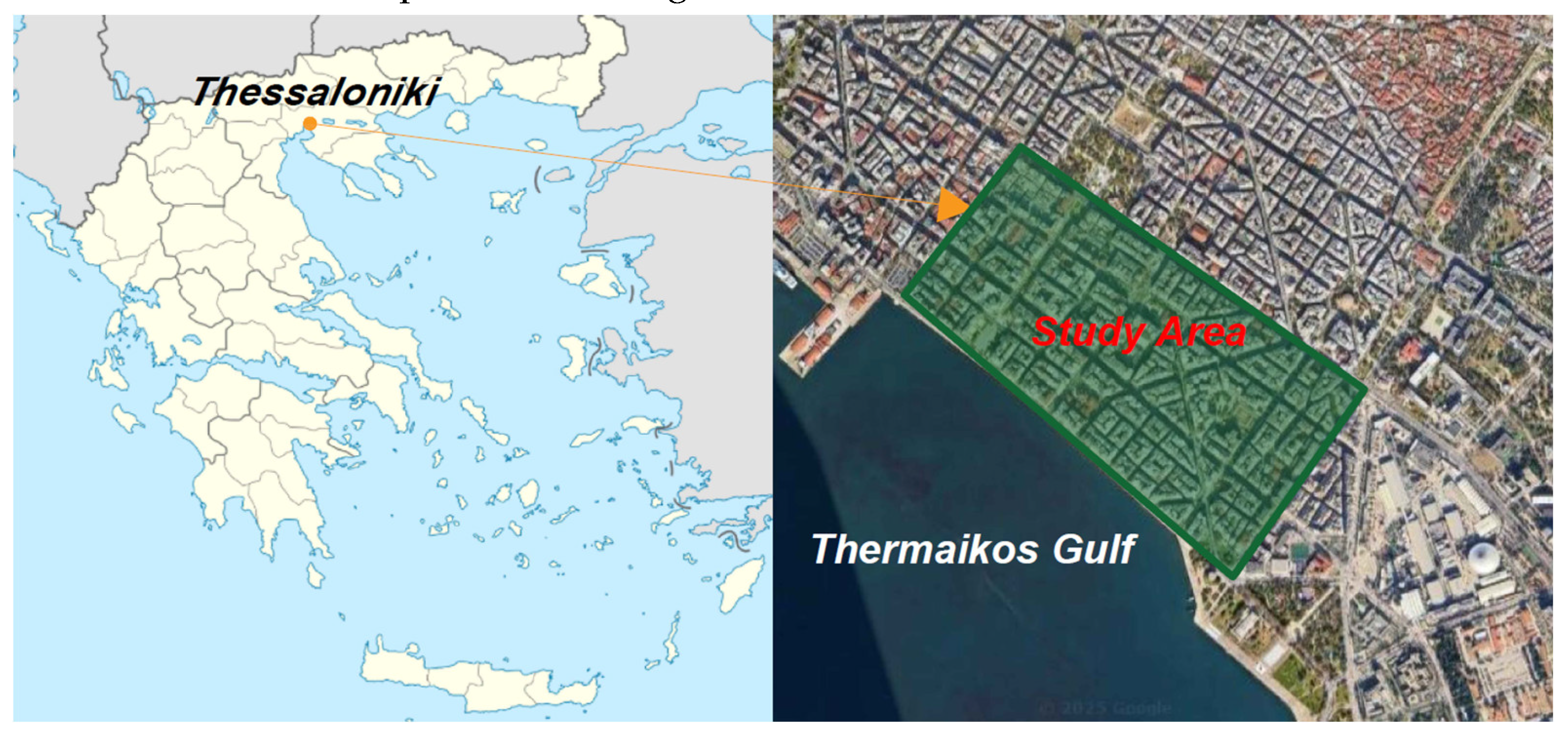
Figure 2.
Box-and-whisker diagrams of annual maximum daily precipitation for the three climate models in the study area.
Figure 2.
Box-and-whisker diagrams of annual maximum daily precipitation for the three climate models in the study area.
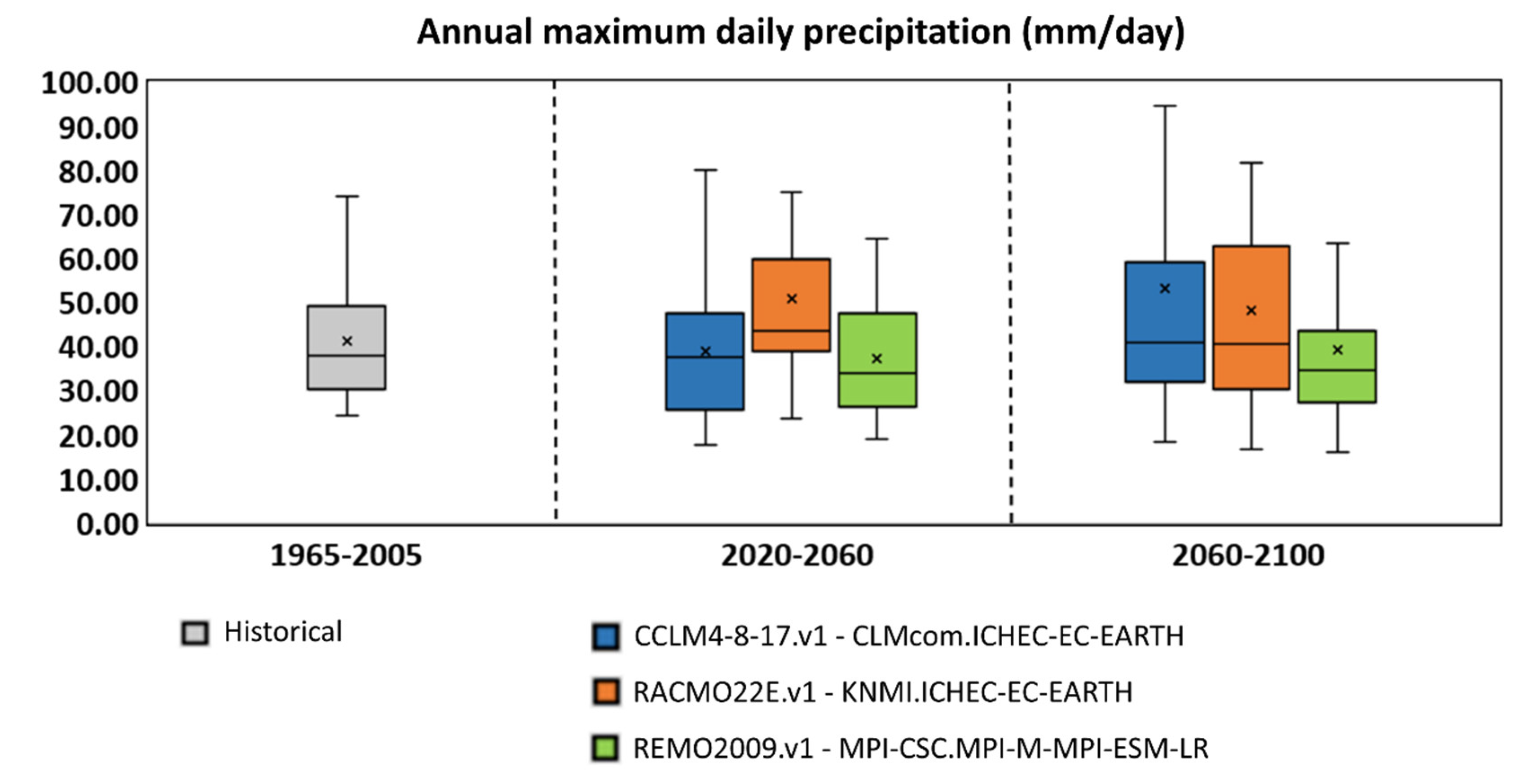
Figure 3.
The log-log plot of GEV NCMs of annual maximum rainfall versus duration at Mikra station, Thessaloniki.
Figure 3.
The log-log plot of GEV NCMs of annual maximum rainfall versus duration at Mikra station, Thessaloniki.
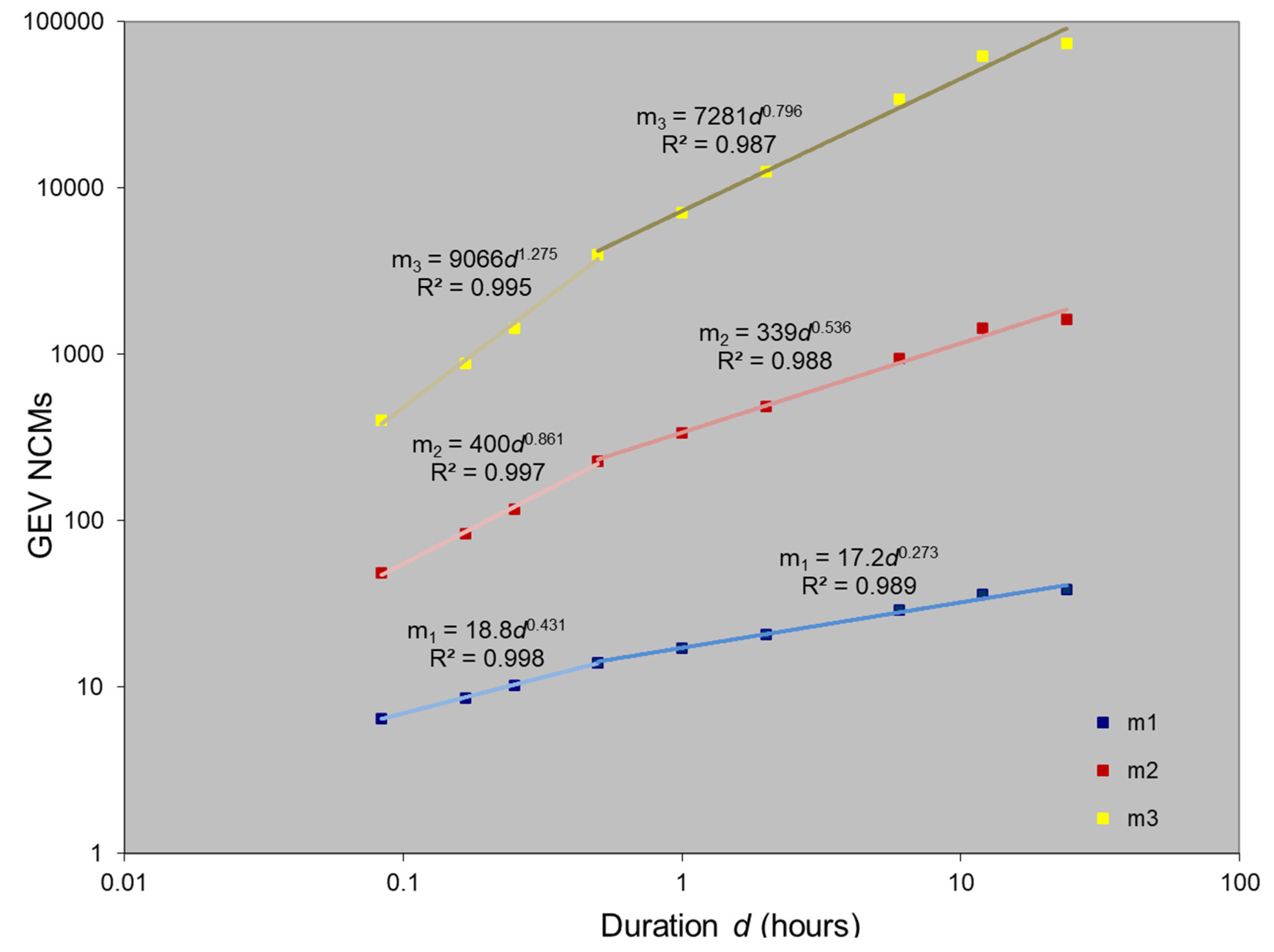
Figure 4.
The scaling exponent β(k) versus the GEV NCM order for the intervals: (a) 5min to 30min, (b) 30min to 1h.
Figure 4.
The scaling exponent β(k) versus the GEV NCM order for the intervals: (a) 5min to 30min, (b) 30min to 1h.
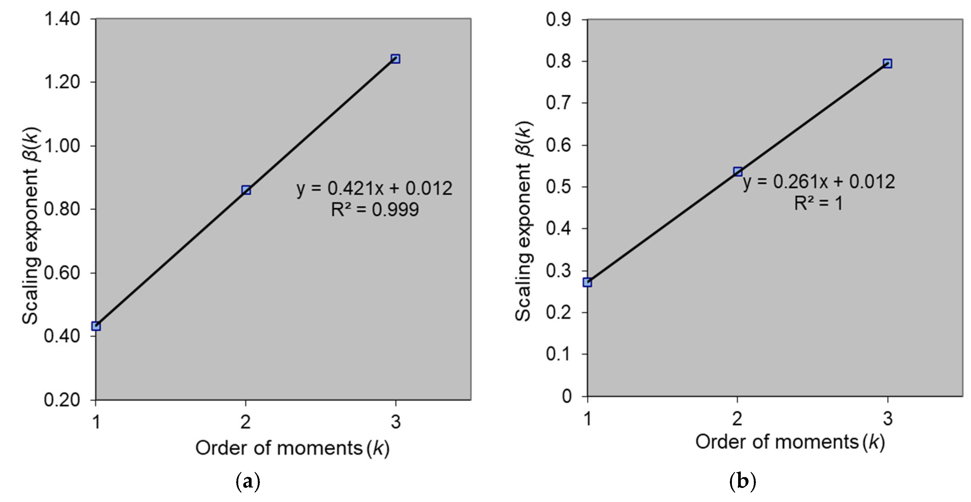
Figure 5.
IDF and DDF curves for the historical/reference period (1965-2005) in Thessaloniki, Greece.
Figure 5.
IDF and DDF curves for the historical/reference period (1965-2005) in Thessaloniki, Greece.
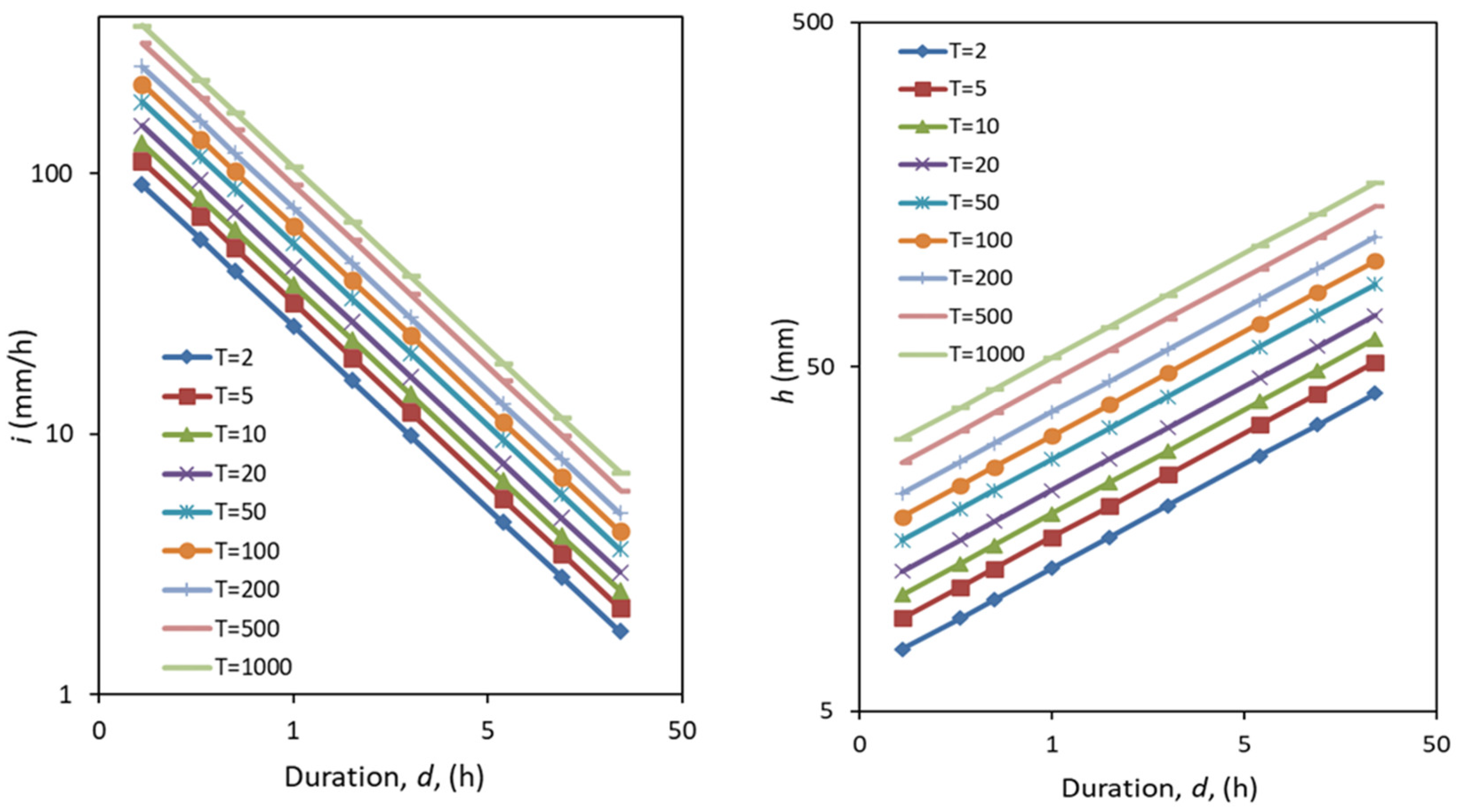
Figure 6.
IDF curves for the future climate in Thessaloniki, Greece: (a) 2020-2060 with CCLM RCM, (b) 2060-2100 with CCLM RCM, (c) 2020-2060 with RACMO RCM, (d) 2060-2100 with RACMO RCM, (e) 2020-2060 with REMO RCM, (f) 2060-2100 with REMO RCM.
Figure 6.
IDF curves for the future climate in Thessaloniki, Greece: (a) 2020-2060 with CCLM RCM, (b) 2060-2100 with CCLM RCM, (c) 2020-2060 with RACMO RCM, (d) 2060-2100 with RACMO RCM, (e) 2020-2060 with REMO RCM, (f) 2060-2100 with REMO RCM.
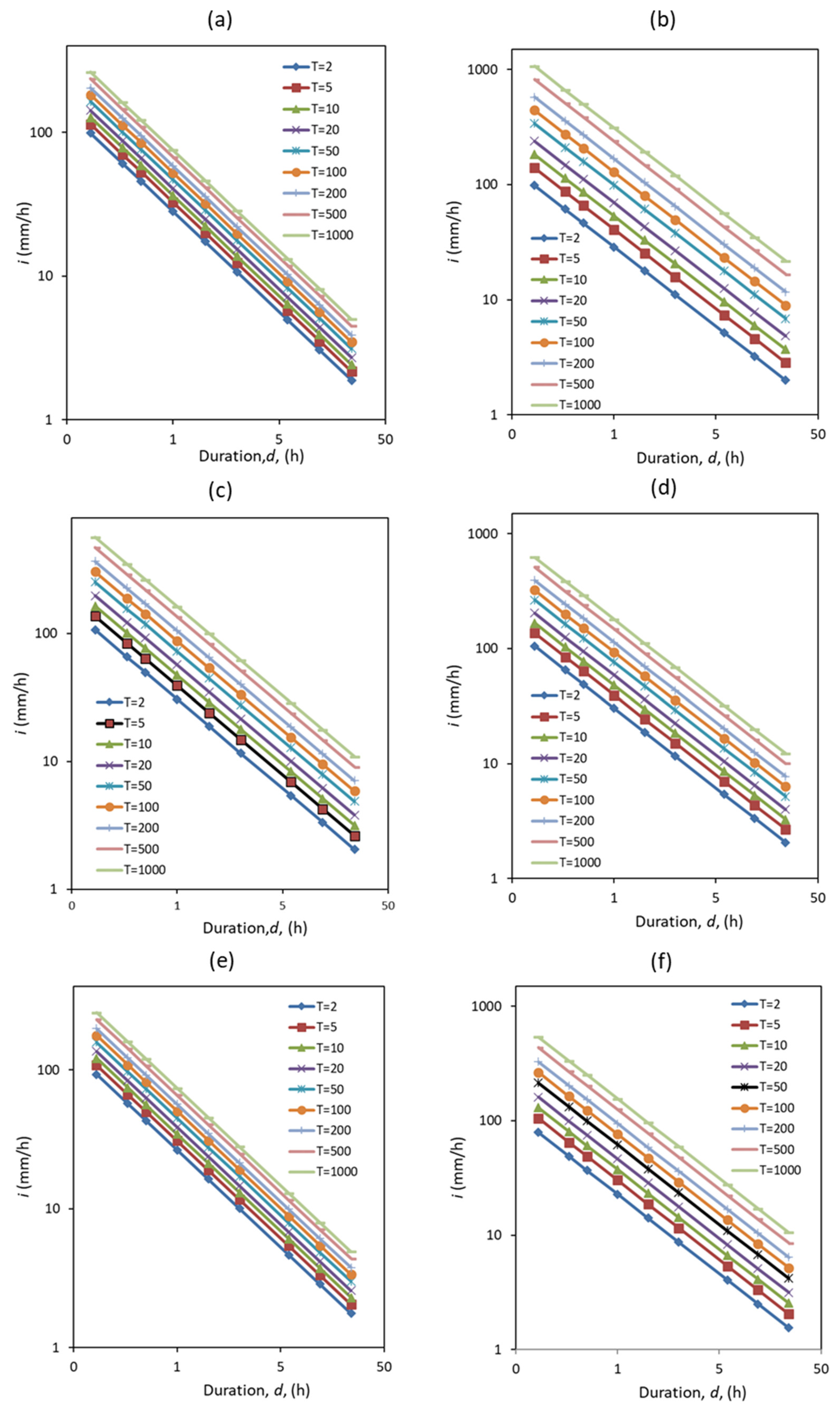
Figure 7.
Hydraulic Results for Existing Conditions under a 100-year Return Period.
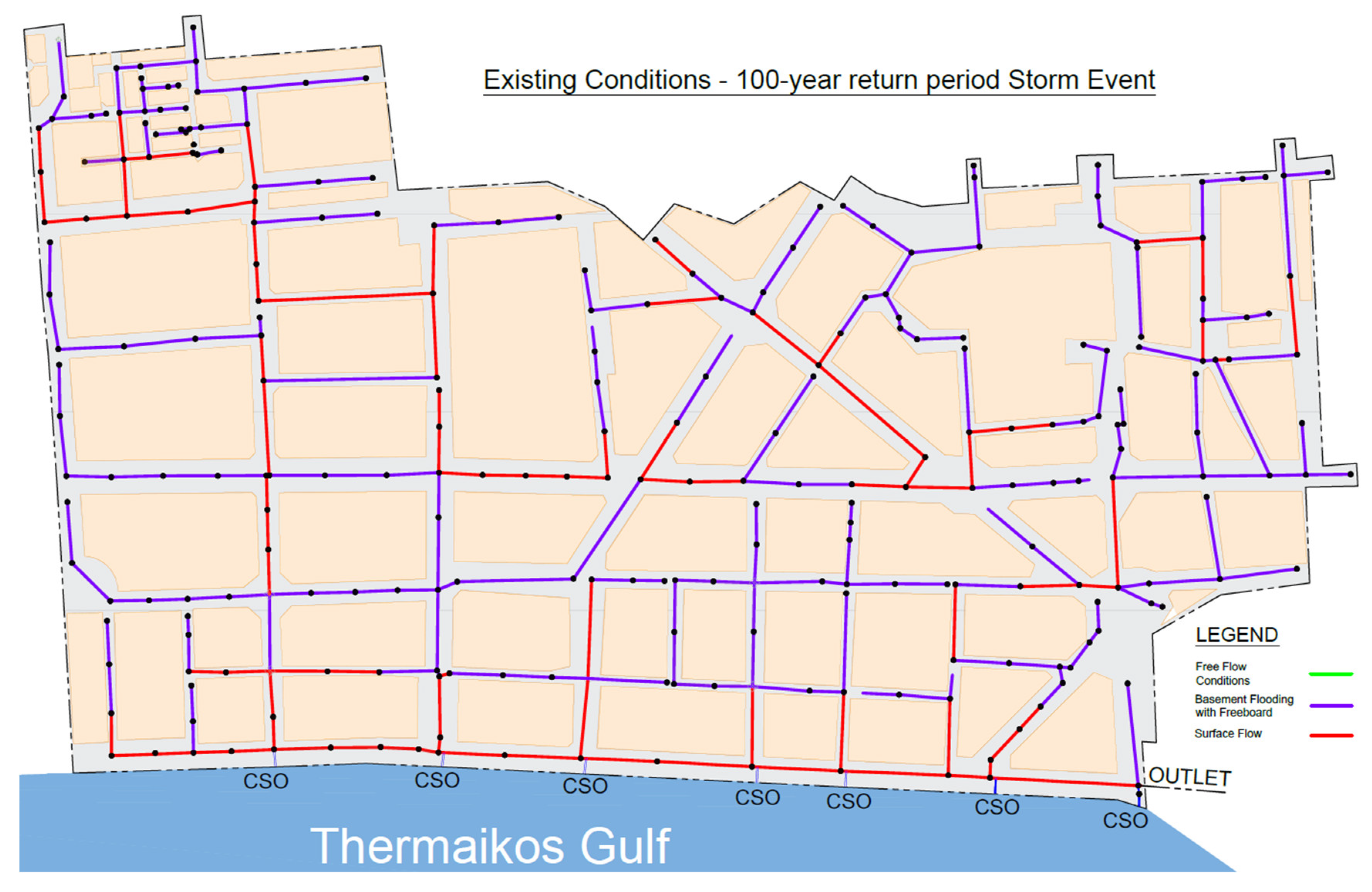
Figure 8.
Hydraulic Results using rainfall distribution derived from CCLM model for a 100-year Return Period during a) 2020-2060 and b) 2060-2100.
Figure 8.
Hydraulic Results using rainfall distribution derived from CCLM model for a 100-year Return Period during a) 2020-2060 and b) 2060-2100.
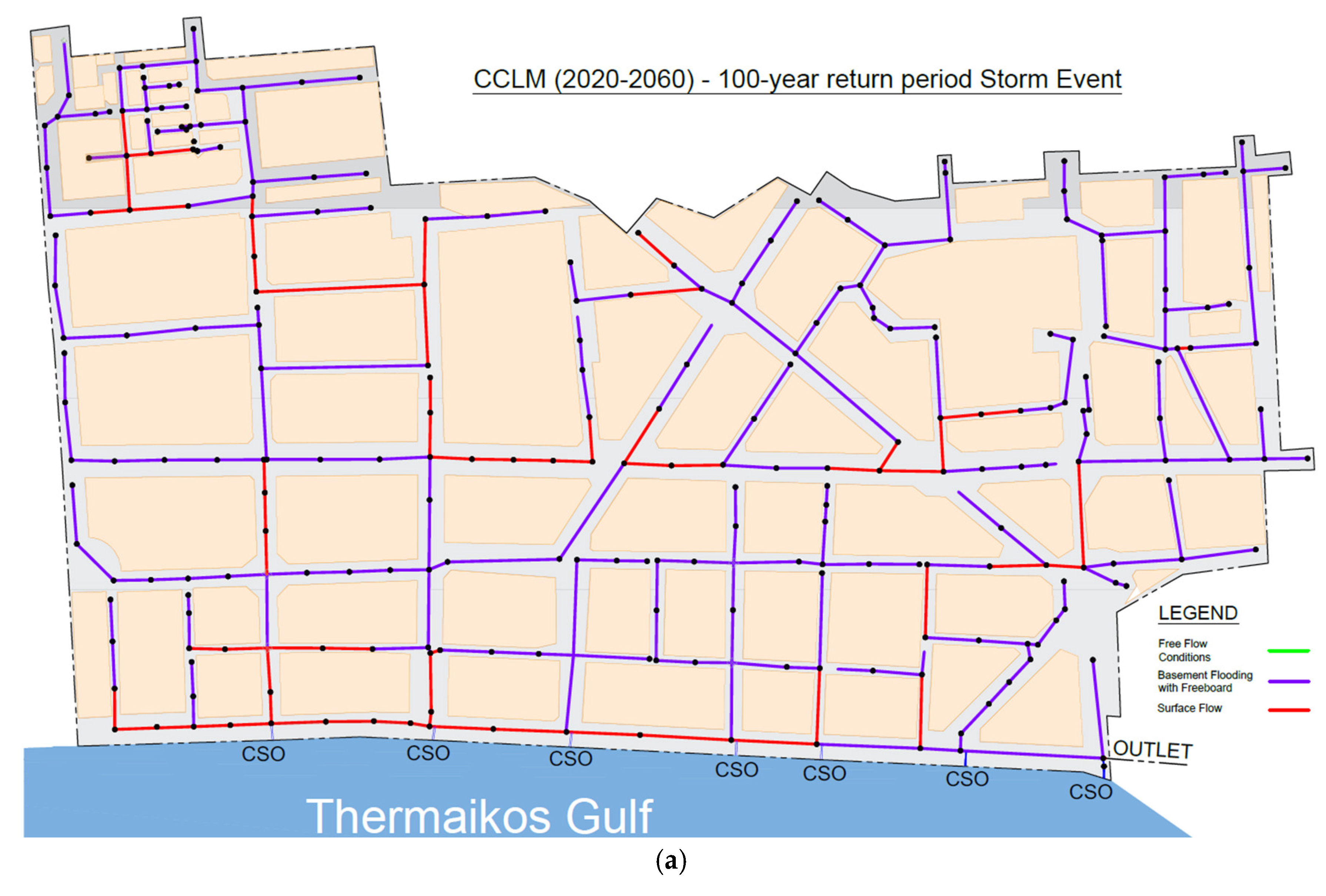
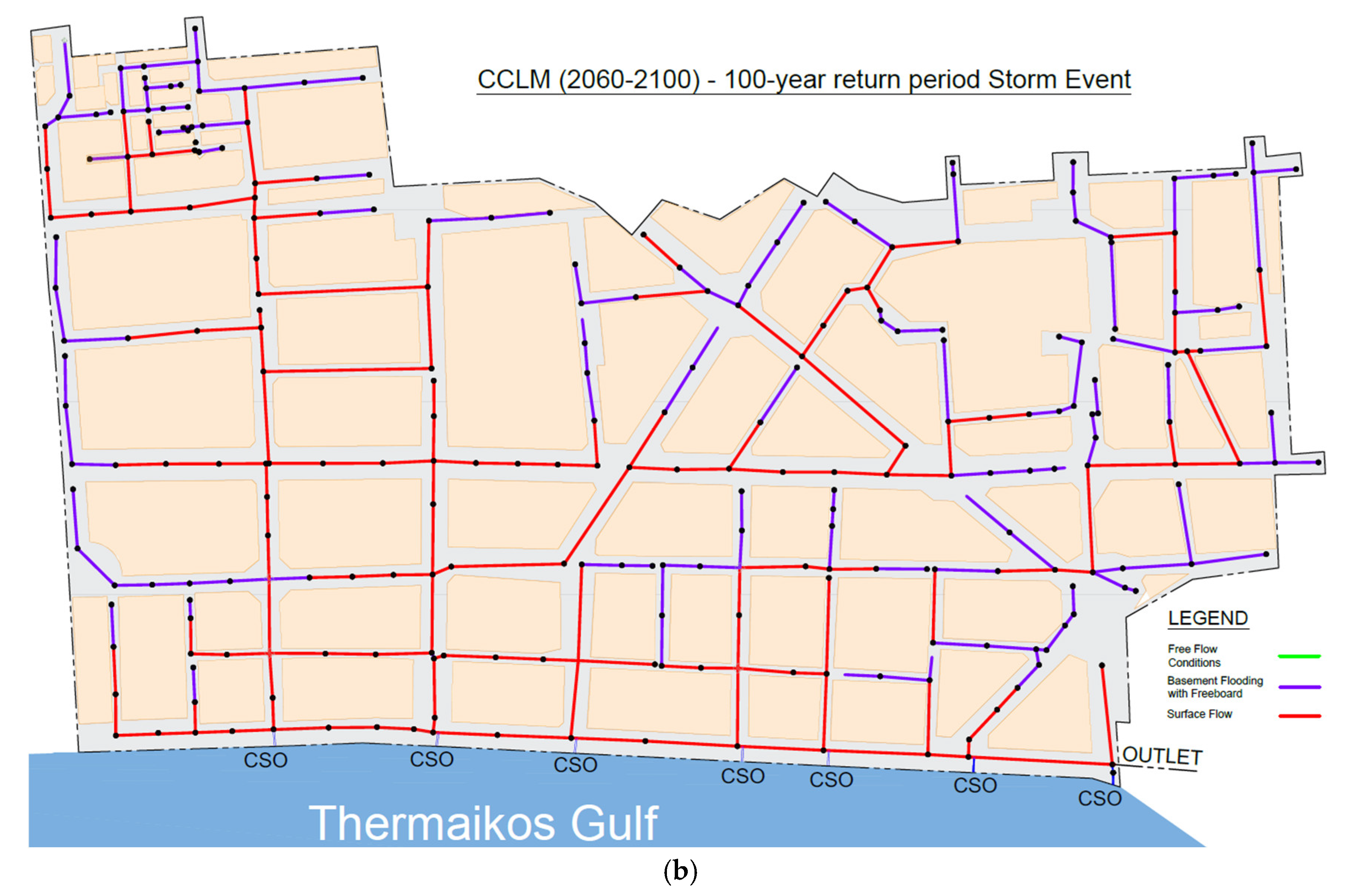
Figure 9.
Hydraulic Results using rainfall distribution derived from RACMO model for a 100-year Return Period during a) 2020-2060 and b) 2060-2100.
Figure 9.
Hydraulic Results using rainfall distribution derived from RACMO model for a 100-year Return Period during a) 2020-2060 and b) 2060-2100.
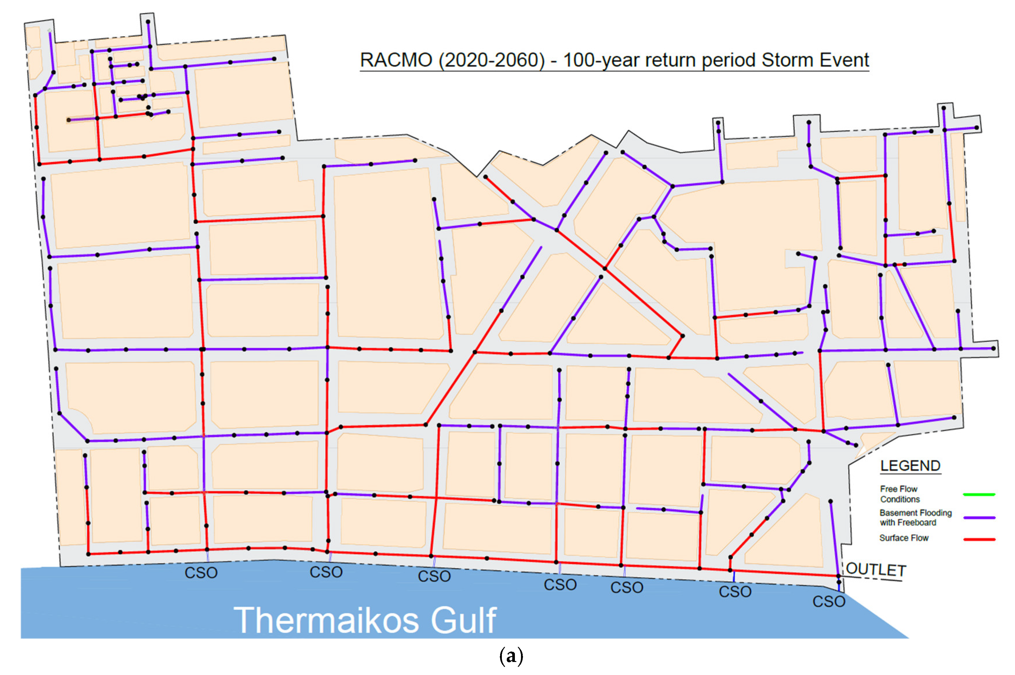
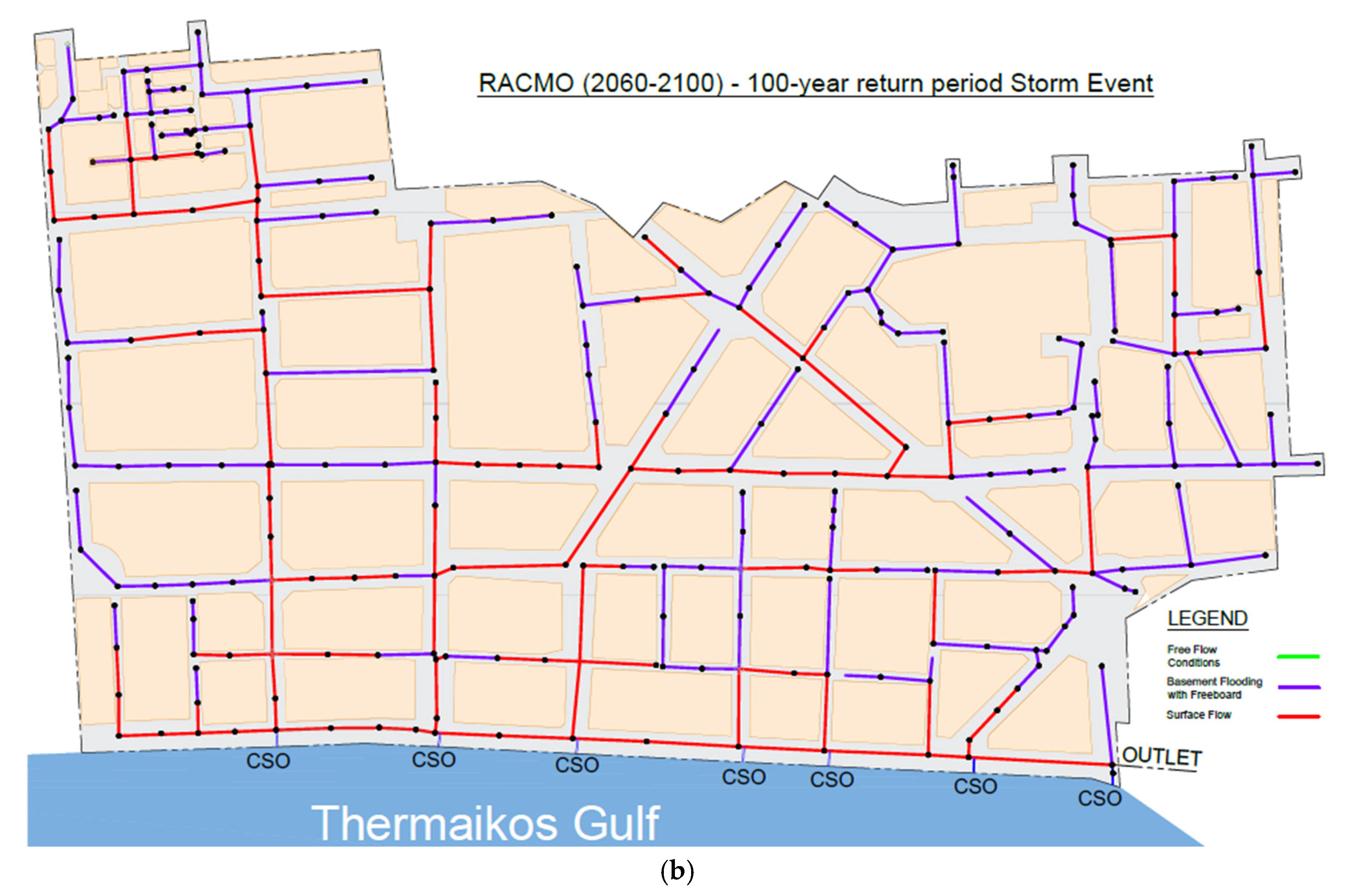
Figure 10.
Hydraulic Results using rainfall distribution derived from REMO model for a 100-year Return Period during a) 2020-2060 and b) 2060-2100.
Figure 10.
Hydraulic Results using rainfall distribution derived from REMO model for a 100-year Return Period during a) 2020-2060 and b) 2060-2100.
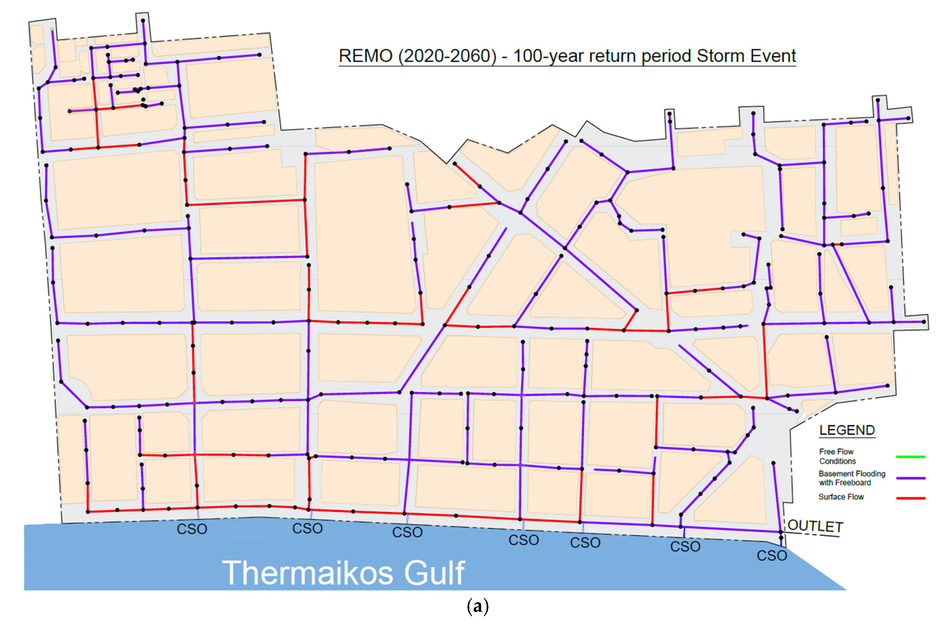
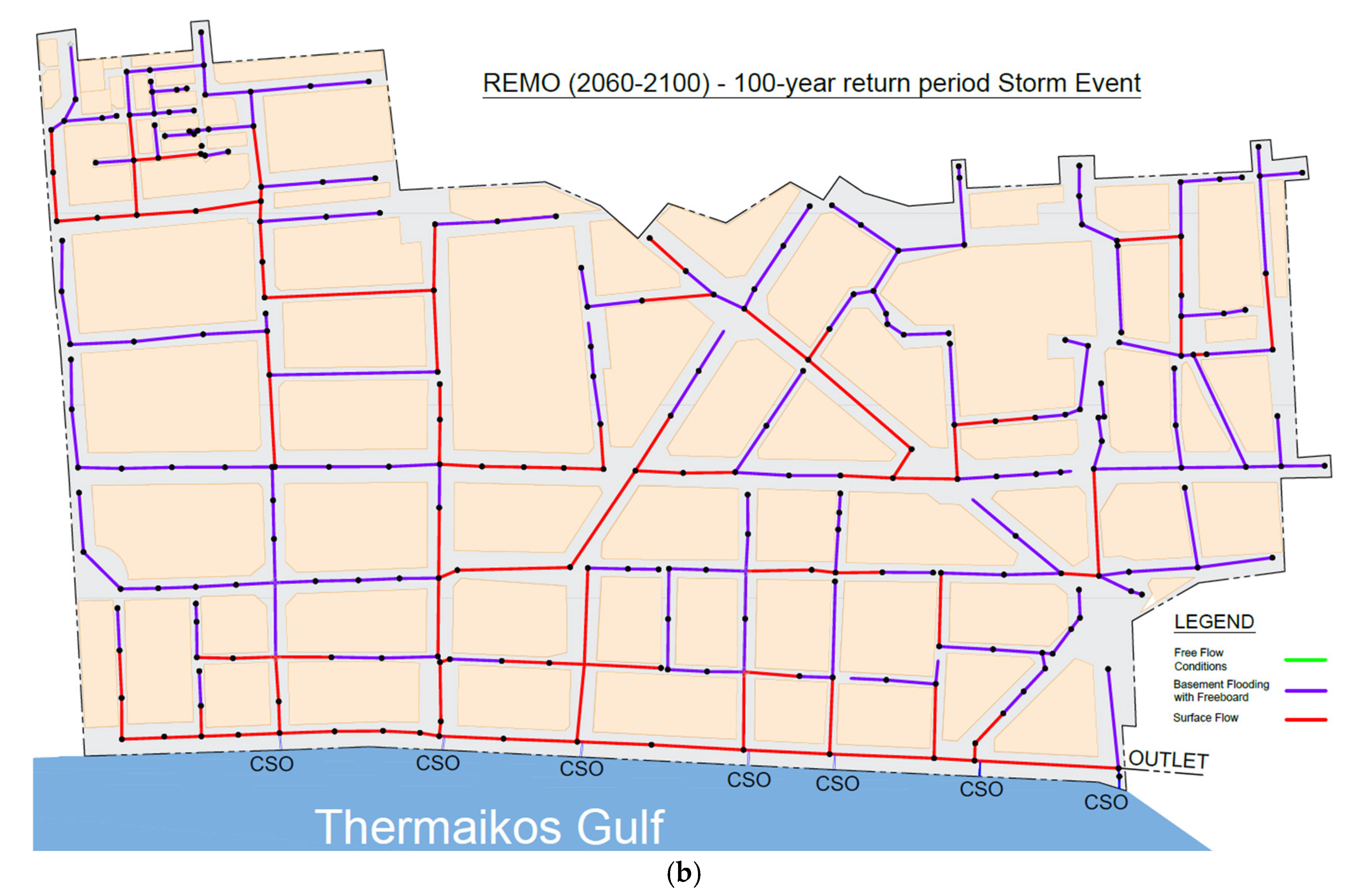

Table 1.
List with the 3 EURO-CORDEX sets of simulations used in the present study.
| Institute_id | RCM | Driving GCM | Realization | |
|---|---|---|---|---|
| 1 | CLMcom | CCLM4-8-17.v1 | CLMcom.ICHEC-EC-EARTH | r12i1p1 |
| 2 | KNMI | RACMO22E.v1 | KNMI.ICHEC-EC-EARTH | r12i1p1 |
| 3 | MPI-CSC | REMO2009.v1 | MPI-CSC.MPI-M-MPI-ESM-LR | r1i1p1 |
Table 2.
Historical precipitation data and future projections based on the CCLM4-8-17.v1 - CLMcom.ICHEC-EC-EARTH climate model.
Table 2.
Historical precipitation data and future projections based on the CCLM4-8-17.v1 - CLMcom.ICHEC-EC-EARTH climate model.
| Measurements (mm/day) (1965-2005) |
Downscaled climatic data (mm/day) (2020-2060) | Downscaled climatic data (mm/day) (2060-2100) | ||||||||||
|---|---|---|---|---|---|---|---|---|---|---|---|---|
| Daily Min. | Daily Max. | Daily Avg. | St. Dev. | Daily Min. | Daily Max. | Daily Avg. | St. Dev. | Daily Min. | Daily Max. | Daily Avg. | St. Dev. | |
| Oct. | 0.00 | 62.70 | 1.31 | 4.68 | 0.00 | 66.28 | 1.20 | 4.51 | 0.00 | 87.92 | 1.21 | 5.09 |
| Nov. | 0.00 | 98.00 | 1.72 | 5.96 | 0.00 | 66.07 | 2.02 | 6.60 | 0.00 | 88.06 | 2.39 | 8.06 |
| Dec. | 0.00 | 54.50 | 1.62 | 4.80 | 0.00 | 35.69 | 1.31 | 2.80 | 0.00 | 22.86 | 1.63 | 2.93 |
| Jan. | 0.00 | 33.80 | 1.11 | 3.34 | 0.00 | 40.59 | 1.22 | 3.73 | 0.00 | 29.21 | 0.86 | 2.96 |
| Feb. | 0.00 | 49.20 | 1.22 | 3.88 | 0.00 | 46.24 | 1.11 | 3.48 | 0.00 | 33.76 | 0.89 | 2.70 |
| Mar. | 0.00 | 49.00 | 1.23 | 3.82 | 0.00 | 31.82 | 1.11 | 3.02 | 0.00 | 38.83 | 1.26 | 3.71 |
| Apr. | 0.00 | 54.20 | 1.25 | 3.85 | 0.00 | 35.74 | 1.16 | 3.43 | 0.00 | 34.90 | 0.85 | 3.01 |
| May | 0.00 | 38.10 | 1.53 | 4.32 | 0.00 | 51.25 | 1.56 | 3.91 | 0.00 | 86.33 | 1.67 | 4.89 |
| June | 0.00 | 39.60 | 0.89 | 3.47 | 0.00 | 63.64 | 1.06 | 4.19 | 0.00 | 109.21 | 1.11 | 4.78 |
| July | 0.00 | 60.70 | 0.92 | 4.37 | 0.00 | 49.77 | 1.03 | 4.18 | 0.00 | 155.29 | 0.86 | 5.48 |
| Aug. | 0.00 | 36.10 | 0.78 | 3.36 | 0.00 | 79.82 | 0.64 | 3.78 | 0.00 | 185.40 | 0.73 | 6.37 |
| Sept. | 0.00 | 50.90 | 0.93 | 3.93 | 0.00 | 56.68 | 0.92 | 3.47 | 0.00 | 53.08 | 0.73 | 3.30 |
Table 3.
Historical precipitation data and future projections based on the RACMO22E.v1 - KNMI.ICHEC-EC-EARTH climate model.
Table 3.
Historical precipitation data and future projections based on the RACMO22E.v1 - KNMI.ICHEC-EC-EARTH climate model.
| Measurements (mm/day) (1965-2005) |
Downscaled climatic data (mm/day) (2020-2060) | Downscaled climatic data (mm/day) (2060-2100) | ||||||||||
|---|---|---|---|---|---|---|---|---|---|---|---|---|
| Daily Min. | Daily Max. | Daily Avg. | St. Dev. | Daily Min. | Daily Max. | Daily Avg. | St. Dev. | Daily Min. | Daily Max. | Daily Avg. | St. Dev. | |
| Oct. | 0.00 | 62.70 | 1.31 | 4.68 | 0.00 | 68.74 | 1.32 | 5.19 | 0.00 | 60.94 | 1.06 | 4.09 |
| Nov. | 0.00 | 98.00 | 1.72 | 5.96 | 0.00 | 105.42 | 2.51 | 8.75 | 0.00 | 79.22 | 2.33 | 8.18 |
| Dec. | 0.00 | 54.50 | 1.62 | 4.80 | 0.00 | 41.35 | 1.31 | 4.12 | 0.00 | 74.02 | 1.97 | 5.66 |
| Jan. | 0.00 | 33.80 | 1.11 | 3.34 | 0.00 | 28.49 | 1.04 | 2.56 | 0.00 | 19.63 | 0.74 | 2.07 |
| Feb. | 0.00 | 49.20 | 1.22 | 3.88 | 0.00 | 45.52 | 1.67 | 4.81 | 0.00 | 45.84 | 1.38 | 4.30 |
| Mar. | 0.00 | 49.00 | 1.23 | 3.82 | 0.00 | 92.80 | 1.56 | 4.88 | 0.00 | 45.06 | 1.48 | 4.49 |
| Apr. | 0.00 | 54.20 | 1.25 | 3.85 | 0.00 | 41.94 | 1.10 | 3.23 | 0.00 | 46.96 | 1.18 | 3.92 |
| May | 0.00 | 38.10 | 1.53 | 4.32 | 0.00 | 72.92 | 2.00 | 5.45 | 0.00 | 70.56 | 1.89 | 5.74 |
| June | 0.00 | 39.60 | 0.89 | 3.47 | 0.00 | 38.82 | 0.99 | 3.21 | 0.00 | 55.75 | 1.08 | 3.92 |
| July | 0.00 | 60.70 | 0.92 | 4.37 | 0.00 | 49.77 | 1.03 | 4.18 | 0.00 | 155.29 | 0.86 | 5.48 |
| Aug. | 0.00 | 36.10 | 0.78 | 3.36 | 0.00 | 30.92 | 0.53 | 2.09 | 0.00 | 29.74 | 0.79 | 2.75 |
| Sept. | 0.00 | 50.90 | 0.93 | 3.93 | 0.00 | 100.90 | 1.26 | 5.54 | 0.00 | 81.47 | 1.09 | 4.71 |
Table 4.
Historical precipitation data and future projections based on the REMO2009.v1 - MPI-CSC.MPI-M-MPI-ESM-LR climate model.
Table 4.
Historical precipitation data and future projections based on the REMO2009.v1 - MPI-CSC.MPI-M-MPI-ESM-LR climate model.
| Measurements (mm/day) (1965-2005) |
Downscaled climatic data (mm/day) (2020-2060) | Downscaled climatic data (mm/day) (2060-2100) | ||||||||||
|---|---|---|---|---|---|---|---|---|---|---|---|---|
| Daily Min. | Daily Max. | Daily Avg. | St. Dev. | Daily Min. | Daily Max. | Daily Avg. | St. Dev. | Daily Min. | Daily Max. | Daily Avg. | St. Dev. | |
| Oct. | 0.00 | 62.70 | 1.31 | 4.68 | 0.00 | 49.09 | 1.29 | 4.15 | 0.00 | 36.25 | 1.18 | 3.47 |
| Nov. | 0.00 | 98.00 | 1.72 | 5.96 | 0.00 | 64.50 | 1.90 | 6.11 | 0.00 | 63.37 | 2.01 | 6.15 |
| Dec. | 0.00 | 54.50 | 1.62 | 4.80 | 0.00 | 54.92 | 1.87 | 5.43 | 0.00 | 56.46 | 1.54 | 4.93 |
| Jan. | 0.00 | 33.80 | 1.11 | 3.34 | 0.00 | 31.16 | 1.21 | 3.36 | 0.00 | 40.98 | 1.22 | 3.60 |
| Feb. | 0.00 | 49.20 | 1.22 | 3.88 | 0.00 | 59.89 | 1.24 | 3.91 | 0.00 | 55.69 | 1.39 | 4.51 |
| Mar. | 0.00 | 49.00 | 1.23 | 3.82 | 0.00 | 52.69 | 1.51 | 4.55 | 0.00 | 29.66 | 1.05 | 3.11 |
| Apr. | 0.00 | 54.20 | 1.25 | 3.85 | 0.00 | 38.33 | 1.29 | 3.67 | 0.00 | 39.17 | 1.32 | 3.90 |
| May | 0.00 | 38.10 | 1.53 | 4.32 | 0.00 | 32.42 | 1.18 | 3.13 | 0.00 | 31.66 | 0.88 | 2.50 |
| June | 0.00 | 39.60 | 0.89 | 3.47 | 0.00 | 27.13 | 0.52 | 1.92 | 0.00 | 146.11 | 0.70 | 4.68 |
| July | 0.00 | 60.70 | 0.92 | 4.37 | 0.00 | 52.09 | 0.53 | 2.94 | 0.00 | 61.20 | 0.40 | 2.73 |
| Aug. | 0.00 | 36.10 | 0.78 | 3.36 | 0.00 | 49.81 | 0.61 | 2.83 | 0.00 | 50.13 | 0.52 | 2.55 |
| Sept. | 0.00 | 50.90 | 0.93 | 3.93 | 0.00 | 28.59 | 0.80 | 3.10 | 0.00 | 42.30 | 0.59 | 2.77 |
Table 5.
IDF and DDF curve equations for the historical and future climate in Thessaloniki, Greece.
| Climate Period & RCM | DDF equation | IDF equation |
|---|---|---|
| 1965-2005 Historical/Reference | 33.19T0.227d0.302 | 33.19T0.227d-0.698 |
| 2020-2060 CCLM | 28.83T0.157d0.300 | 28.83T0.157d-0.700 |
| 2020-2060 RACMO | 44.70T0.268d0.303 | 44.70T0.268d-0.697 |
| 2020-2060 REMO | 27.73T0.165d0.300 | 27.73T0.165d-0.700 |
| 2060-2100 CCLM | 61.24T0.383d0.311 | 61.24T0.383d-0.689 |
| 2060-2100 RACMO | 47.13T0.287d0.306 | 47.13T0.287d-0.694 |
| 2060-2100 REMO | 38.02T0.309d0.305 | 38.02T0.309d-0.695 |
Table 6.
Combined sewer system performance under historical and future climate in Thessaloniki, Greece.
Table 6.
Combined sewer system performance under historical and future climate in Thessaloniki, Greece.
| Scenario (100-year return period) |
Combined Sewer Overflow Volume (m3) |
|---|---|
| Existing Conditions | 12,273 |
| 2020-2060 CCLM | 10,735 |
| 2020-2060 RACMO | 17,117 |
| 2020-2060 REMO | 10,012 |
| 2060-2100 CCLM | 25,514 |
| 2060-2100 RACMO | 18,605 |
| 2060-2100 REMO | 15,799 |
Disclaimer/Publisher’s Note: The statements, opinions and data contained in all publications are solely those of the individual author(s) and contributor(s) and not of MDPI and/or the editor(s). MDPI and/or the editor(s) disclaim responsibility for any injury to people or property resulting from any ideas, methods, instructions or products referred to in the content. |
© 2025 by the authors. Licensee MDPI, Basel, Switzerland. This article is an open access article distributed under the terms and conditions of the Creative Commons Attribution (CC BY) license (http://creativecommons.org/licenses/by/4.0/).
Copyright: This open access article is published under a Creative Commons CC BY 4.0 license, which permit the free download, distribution, and reuse, provided that the author and preprint are cited in any reuse.


