
Submitted:
24 February 2025
Posted:
24 February 2025
You are already at the latest version
Abstract
The aging effect will weaken the capacity of lithium batteries and seriously affect the performance of electric vehicles. Developing State of Health estimation technology for lithium batteries can help optimize the charging and discharging strategies of electric vehicles. This study investigates the use of partial discharge data for SOH estimation. To overcome the limitation of unstable output of traditional estimation models caused by partial discharge data in low voltage scenarios. This study first used the DoppelGANger network to generate artificially synthesized data. After the data augmentation process, train the Temporal Convolutional Network to construct a data-driven SOH model. Finally, the performance of the SOH model output is evaluated using three indicators: RMSE, MAPE, and delta. The proposed method improved 5 kinds of low-voltage operating conditions in 7 testing scenarios compared with traditional SOH estimation models. The experimental results provide a practical solution for data-driven SOH estimation.
Keywords:
lithium battery
; State of Health
; DoppelGANger network
; Temporal Convolutional Network
1. Introduction
With the rapid development of electric vehicles (EVs), the demand for high-performance battery systems is increasing. As one of the core components of electric vehicles, Battery Management System (BMS) is crucial for ensuring the safety, reliability, and lifespan of batteries. However, as the aging effect, battery degradation is inevitable, which can lead to a decrease in battery performance and a shortened lifespan. Among the multiple functions of BMS, accurate estimation of State of Health (SOH) and Remaining Useful Life (RUL) is the key issue to achieving efficient battery management [1,2,3].
Considering that the aging of lithium batteries leads to an increase in internal resistance, which in turn reduces battery capacity and seriously affects the performance of electric vehicles. Developing SOH estimation technology not only helps optimize charging and discharging strategies but also extends the lifespan of batteries. A comprehensive review of modeling and state estimation methods for lithium batteries is presented in [4]. At present, SOH estimation techniques are divided into experimental-based and model-based methods.
Sun et al. proposed a SOH estimation technique based on Electrochemical Impedance Spectroscopy (EIS) [5]. EIS analyzes the internal electrochemical processes of lithium batteries by examining their impedance response at different frequencies. EIS can effectively characterize key parameters such as electrode reaction kinetics, electrolyte diffusion characteristics, and interface stability of batteries. By comparing the impedance spectra of different aging stages, the variation in the internal structure of the battery can be observed, furthermore providing for the evaluation of SOH. Due to the non-destructive testing and condition monitoring characteristics, EIS technology is suitable for online monitoring and diagnosis of SOH [6].
For model-based SOH estimation methods: Demirci et al. monitor the physical characteristics and operational data of batteries in real-time (such as voltage, current, temperature, etc.), then use data-driven models to estimate the SOH of batteries [7]. Incremental capacity analysis (ICA) is another SOH estimation technique. The ICA method can identify the aging characteristics of the battery and predict the remaining service life by analyzing the incremental capacity curve of the battery. The strategy of combining ICA with support vector regression has shown high reliability in practical applications [8].
To improve the limitation of estimation model, which requires a precise load curve, Shu et al. proposed an online diagnosis method based on short-term charging curves [9]. The method utilizes the voltage curve characteristics to evaluate the SOH through machine learning algorithms. Experimental results have confirmed that the shape of the charging curve during the initial charging stage is closely related to their degree of aging. By training the SOH model, the proposed method can determine the SOH in a short time. The method based on partial charge/discharge curves provides a feasible technical means for real-time estimation of the battery for electric vehicles.
The electrochemical model of lithium batteries can describe the electrochemical reaction processes inside the battery. The electrochemical model, combined with data-driven prediction algorithms, can overcome the uncertainty and noise in the model and further achieve dynamic estimation of RUL. The RUL model for lead-acid batteries using the particle filtering algorithm combined with the electrochemical model is studied in [10]. The experimental results provide a new approach for lithium battery models, which is to compensate for the disadvantages of a single method by integrating physical models with data-driven methods.
Gou et al. proposed another hybrid data-driven approach based on deep learning algorithms for SOH estimation and RUL prediction of lithium-ion batteries [11]. The proposed method combines multiple data features, including voltage, current, and temperature information, and utilizes deep learning algorithms such as convolutional neural networks (CNN) and long short-term memory networks (LSTM) for modeling. Research has illustrated that hybrid data-driven methods can effectively improve prediction accuracy while reducing model complexity.
The traditional SOH estimation method usually relies on whole charge/ discharge profiles. However, obtaining complete data is often time-consuming and inconvenient. In practice, EVs require real-time battery data to meet complex operating conditions. Much research is dedicated to estimating SOH through partial charging and discharging profiles to reduce the demand for data acquisition [12,13]. Although the Temporal Convolutional Network (TCN) is widely used for SOH estimation based on partial data, the SOH model of TCN is not ideal at low voltage conditions [14]. More research is needed to improve the robustness of SOH model at low voltage conditions.
Another challenge of the SOH model estimation is the relatively small number of samples available for model training. The data-driven approach relies on the quality and quantity of the dataset, and appropriate data augmentation can often achieve more efficient predictive performance. Reference [15] applied the data generation algorithms to solve the problem of data imbalance in bearing failure and improved the accuracy of failure classification. On the other hand, the data augment skill was utilized for the tire wear data set which is difficult to collect in [16]. Using data augment algorithms to improve the accuracy and robustness of SOH estimation is a feasible research solution.
Based on the above analysis, this study proposes an SOH estimation model that combines DoppelGANger and TCN networks. Firstly, the experimental data of 7 aging conditions are preprocessed to divide the discharge profile into 4 segments of partial SOC data. To address the limited data of aging battery samples, a high-quality artificially synthesized dataset is generated through data augmentation methods. The TCN networks of the experimental group (including the artificially synthesized samples) and the control group are constructed into the data-driven SOH models. Finally, the accuracy and robustness of the SOH model are evaluated using three indicators: RMSE, MAPE, and delta. Compared with traditional SOH estimation models, the proposed method not only improves the estimation accuracy in high-voltage SOC sections but also has good robustness in low-voltage SOC sections.
2. The Analysis of Dataset
2.1 Dataset Introduction
This study employs the randomized battery usage dataset provided by NASA’s Prognostics Center of Excellence (PCoE), which is widely used to evaluate data-driven lithium-ion battery (LIB) aging models and provides a reliable benchmark for algorithm performance validation. The dataset includes aging data for 28 lithium cobalt oxide (LCO) 18650 cells, each with a nominal capacity of approximately 2.1 to 2.2 Ah, as detailed in Table 1. Based on the testing conditions, the dataset is divided into seven groups, each containing data from four cells. Groups 1 to 5 were cycled at room temperature, while Groups 6 and 7 were cycled at an ambient temperature of 40 °C.
To replicate real-world applications, the batteries were subjected to randomized load profiles during charging and discharging. The profiles are referred to here as a random walk (RW) discharging. The specific groupings and test conditions are summarized in Table 2. The aging tests were performed periodically, during which the voltage, current, and temperature of the cells were recorded. After a predetermined number of cycles, a constant-current discharge test was conducted to collect reference discharge data, which was used to characterize the SOH of the batteries. Figure 1 illustrates a sample of the voltage, current, and temperature data recorded during the first 10 cycles for a single cell. The dataset has been processed and is provided in .mat format. The experiment continued until the SOH of the cells dropped to a range between 50% and 80%.
The aging tests were conducted in periodic cycles, during which the voltage, current, and temperature of the batteries were recorded. After a few cycles, a constant-current discharge test was performed to collect reference discharge data. This reference discharge data was used to characterize the SOH of the batteries. Figure 1 provides an example of the voltage, current, and temperature data recorded during the first 10 RW cycles of a single cell. The dataset was made available in .mat format. The entire experiment continued until the batteries' SOH degraded to between 50% and 80%.
2.2. Definition of SOH
Since the original dataset does not directly provide SOH data, the SOH is evaluated using the reference full discharge profiles (from 100% to 0% discharge) to calculate the battery capacity. Coulomb counting (CC) is employed for current integration, resulting in SOHQ, which represents the battery's health status based on capacity degradation. The definition is as follows:
 where Q(t0) represents the capacity of the battery at the beginning of its life, and Q(ti) denotes the capacity at time ti. The maximum SOH value is defined as 100%, serving as a metric to quantify the battery's aging process.
2.3. Partial Discharge Profiles
In real-world applications, the randomness and dynamic nature of battery usage often make it challenging to obtain complete discharge profiles. Partial discharge profiles are more practical and valuable for real-world scenarios. To simulate SOH estimation using partial profiles, the complete discharge profiles were segmented based on different SOC ranges. The SOC and corresponding voltage ranges for various use cases are presented in Table 3. To visually demonstrate the segmentation of partial discharge profiles for different use cases, all reference discharge profiles of Cell 1 from Group 1 throughout the testing process were plotted, as shown in Figure 2.
3. Data Augment by DoppelGANger (DG)
To augment the limited battery sample data and generate a high-quality synthetic dataset, we employed a Generative Adversarial Network (GAN) to enhance the dataset. GAN is a powerful generative model that leverages the adversarial interaction between a Generator (G) and a Discriminator (D). The structure of GAN model is shown in Figure 3.
The Generator (G) is responsible for generating synthetic data from random noise that resembles the real data distribution. The Discriminator (D), on the other hand, determines whether the input data is real or generated by the Generator.
Their objectives are defined by a loss function, as shown in Equation (2):

Here, pdata(x) represents the distribution of real data, pz(z) denotes the distribution of random noise, and G(z) is the output of the Generator, i.e., the generated data.
Traditional GANs are primarily designed for static images or non-sequential data, and their direct application to time-series data may result in generated outputs lacking temporal dependencies. To better generate time-series data with dynamic characteristics, researchers have proposed various GAN models tailored for time-series data, such as RCGAN and TimeGAN. Considering that the current data used for SOH estimation exhibits long-term temporal dependencies, this study adopts DoppelGANger (DG), one of the most effective methods for handling long time-series data.
The overall architecture of DG, as shown in Figure 4, comprises a metadata generator, a time-series generator, an auxiliary discriminator, and a standard discriminator. The specific structure is described as follows:
3.1. Metadata Generator
The metadata generator employs a multi-layer perceptron (MLP) model to generate high-dimensional metadata associated with the time series. The generated metadata not only satisfies the statistical characteristics of the real distribution but also serves as conditional input for the time-series generator, guiding the generation process.
3.2. Time Series Generator
The time-series generator is built on a recurrent neural network (RNN) and is responsible for sequentially generating time-series data. Its input includes random noise and metadata generated by the metadata generator. To enhance the ability to capture long-term dependencies, the generator adopts a batch generation method, producing multiple consecutive time steps of data at once, which significantly reduces the computational complexity required for generating long sequences.
3.3. Discriminator
The standard discriminator distinguishes between generated and real time-series data, guiding the optimization of the time-series generator through an adversarial loss function. To further improve the quality of metadata generation, DG incorporates an auxiliary discriminator dedicated to verifying whether the metadata matches the real distribution. The joint optimization of the two discriminators ensures the fidelity of the joint distribution of time-series data and metadata.
3.4. Normalization Mechanism and Mode Collapse Prevention
DG introduces an adaptive normalization mechanism that normalizes each time series individually, with normalization parameters (e.g., maximum and minimum values) included as part of the metadata. This design effectively mitigates the mode collapse problem commonly encountered in traditional GANs when dealing with data with varying ranges, ensuring the diversity and authenticity of the generated data.
4. Estimation of SOH Through Temporal Convolutional Network (TCN)
In recent years, convolutional architectures have achieved high accuracy in processing sequential data such as audio and translation. Considering the small sample characteristics of partial discharge sequence data used for SOH estimation, this study adopts the Temporal Convolutional Network (TCN) to perform SOH estimation, leveraging best practices from convolutional architectures in other fields.
Temporal Convolutional Network (TCN) is a time-series modeling approach based on Convolutional Neural Networks (CNNs), specifically designed to handle time-series data or tasks with sequential dependencies. By combining causal convolution and dilated convolution, TCN efficiently captures long-term dependencies in sequences while benefiting from parallel computation.
Compared to traditional RNN architectures, the TCN model features parameter sharing, lower memory requirements for training, and faster training speeds, making it more suitable for implementation in BMS. Figure 5 illustrates the TCN network architecture used in this study. The specific structure is described as follows:
4.1. Dilated Convolutional Networks
Dilated convolution significantly enlarges the receptive field by introducing gaps (i.e., dilation rates) between the convolutional kernels, allowing for efficient capture of long-term dependencies. The dilation rate typically grows exponentially, which enables the model to cover a broader temporal range even with fewer layers.
Compared to traditional convolutions, dilated convolutions maintain a low computational cost while capturing global dependencies. Figure 6 illustrates a dilated convolution with dilation rates of [1,2,4,8]. As shown, for a four-layer network, setting the dilation rates to [1,2,4,8] allows the output at a single time step to be related to data from 16-time steps at the input, significantly expanding the receptive field.
4.2. Causal Convolutional Networks
As shown in Figure 5, causal convolutions ensure that the value at time t from the previous layer only depends on the current and previous values at time t in the next layer. Unlike traditional convolutional neural networks, causal convolutions do not allow access to future data. They are designed with a unidirectional structure, where the “cause” must precede the “effect,” thus introducing a strict temporal constraint. This mechanism prevents information leakage, ensuring the model’s validity for forecasting tasks.
4.3. Residual Blocks
The deeper the network, the stronger its expressive power and better its performance, to a certain extent. However, experiments have shown that when the network depth becomes too large, performance may degrade. In addition to the dilated convolution method, the use of residual connections is also an effective solution to this issue. Residual connections originate from Residual Networks (ResNet), which aim to address the problems of network degradation and vanishing gradients caused by increasing network depth.
Let x be the input to the model, and F(x) be the output after a linear transformation and activation. The formula for this process is as follows:
 where o represents the output, and “Activation” denotes the activation function. This connection process is known as a residual connection, with each connection forming a residual module. Multiple residual modules are combined to form a ResNet.
In this paper, a residual block is designed based on the characteristics of the discharge current sequence, as shown in Figure 5. The residual block consists of two layers of causal dilated convolutions, with ReLU as the activation function. Dropout is employed to mitigate overfitting, and an optional 1×1 convolution is introduced to ensure that the input and output lengths of the residual block are the same.
5. Method and Procedure
The methodology and procedure of proposed method are demonstrated in Figure 7. The procedure consists of five main components: Data Preprocessing, GAN Enhancement, Data Split, TCN Training, and Performance Evaluation.
5.1. Data Preprocessing
To ensure the model’s generalization ability and the reliability of performance evaluation, the limited raw dataset needs to be partitioned. Typically, the dataset is divided into a training set, validation set, and test set. The training set, which constitutes the largest portion of the dataset, is used for the model training process. Data from the training set is utilized to compute the loss function and update the model parameters, allowing the model to learn the mapping between input data and target output.
The validation set is used to monitor the model’s performance during training to prevent overfitting. During training, the model’s performance on the validation set (such as validation loss or accuracy) is used to select the optimal hyperparameters (e.g., learning rate, model structure, etc.). The test set is used for the final evaluation of the model’s generalization performance. The test data remains completely unseen during the model training and hyperparameter tuning phases, and the evaluation results from the test set provide an accurate reflection of the model’s performance in real-world applications.
As introduced in Section 2.1, this study uses the NASA PCoe random battery usage dataset. The dataset is divided into seven groups based on different test conditions, with each group containing data from four batteries. In this study, the first battery in each group is designated as the Test Data (test set), while the remaining three batteries are treated as Raw Data. The Raw Data is further divided into training and validation sets, with details on this division provided in Section 5.3.
5.2. GAN Enhancement
Data-driven algorithms heavily depend on high-quality datasets. To enhance the performance of such algorithms, this study utilizes GAN to augment the limited dataset. The Raw Data, as defined in Section 5.1, is input into the GAN, which generates synthetic data with characteristics and distributions similar to the original data. The synthetic data is then combined with the Raw Data to create an enhanced dataset, referred to as the Enhanced Data.
5.3. Data Split
After data preprocessing and GAN enhancement, we obtain three datasets: Test Data, Raw Data, and Enhanced Data. All three are complete discharge profiles. However, since this study focuses on evaluating SOH using partial discharge profiles, the data needs further segmentation, as described in Section 2.3.
Considering that hyperparameter tuning is required during the training process of the data-driven model, the segmented Raw Data and Enhanced Data are further divided into subsets: Raw Data Train, Raw Data Test, Enhanced Data Train, and Enhanced Data Test. These subsets facilitate the process of hyperparameter optimization.
5.4. TCN Training
This study employs TCN to establish the relationship between partial discharge profiles and the SOH. The TCN takes partial discharge profiles as input and outputs the estimated SOH.
To achieve the best SOH estimation performance, it is essential to determine the optimal model architecture and corresponding weights. This involves training and selecting the approximate function associated with the model structure, along with its corresponding model weights θ , such that:
 where, x represents the input vector, and y denotes the corresponding output values. The model training process utilizes the Adam optimization algorithm to perform the optimization. The loss function selected for this study is the Mean Squared Error (MSE), which is defined as:
 where, represents the model’s output, and n corresponds to the number of samples input into the model.
5.5. Performance Evaluation
To evaluate the SOH estimation method based on GAN-enhanced partial discharge profiles proposed in this study, partial discharge profiles derived from Raw Data and Enhanced Data are used to train and fine-tune the TCN model. The performance of the model is then assessed using profiles from the Test Data, which were not involved in the training or tuning process.
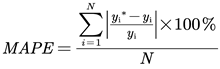
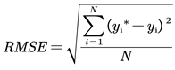
The evaluation involves visualizing the delta curves between the true and predicted values, the Mean Absolute Percentage Error (MAPE), and the Root Mean Squared Error (RMSE). The definitions of the delta value, MAPE, and RMSE are as follows:
6. Experiment and Analysis
6.1. GAN-Based Synthetic Data Generation and Evaluation
This study employs a GAN model to augment the original dataset, specifically adopting the DoppelGANger (DG) model. The implementation is based on Python 3.9.2 and PyTorch 2.5.0. The model training was performed on a computer equipped with an i5-13490F CPU and an Nvidia GeForce GTX 1660 SUPER GPU. The hyperparameters of the DG model are shown in Table 4.
To assess the effectiveness of the synthetic data generated using the DG model, a comparison was made between a set of original data and its synthetic counterpart through visualization. The selected data includes one set of voltage records and one set of current records, as shown in Figure 8 and Figure 9. The red curve on the left represents the original data, while the blue curve on the right corresponds to the synthetic data.
Figure 9 illustrates that the synthetic data generated by the DG model closely resembles the original data, showcasing a good similarity to the original data.Furthermore, to better evaluate the similarity between the generated data and the original data, Principal Component Analysis (PCA) and t-Distributed Stochastic Neighbor Embedding (t-SNE) were employed for visualization.
PCA is a linear dimensionality reduction technique that extracts the principal components of the data. The principle of PCA is mapping high-dimensional data to a lower-dimensional space. As shown in Figure 10, the visualization results indicate that the distribution of the generated data closely aligns with the principal component distribution of the original data, demonstrating that the GAN-generated data captures the overall features of the original data effectively.
t-SNE, on the other hand, is a nonlinear dimensionality reduction method well-suited for handling high-dimensional data and revealing its local structures in a lower-dimensional space. After applying t-SNE, the visualizations reveal that the generated data exhibits a high degree of similarity to the original data in terms of local cluster structures. As illustrated in Figure 10, the t-SNE distribution of the synthetic data closely resembles that of the original data.
The experimental results confirm that the GAN-generated data not only approximates the global distribution of the original data but also achieves a high level of consistency in local structures.
6.2. TCN-Based SOH Estimation Using Partial Discharge Profiles
In this study, the TCN model was employed to estimate the SOH using partial discharge profiles. The TCN implementation was based on Python 3.11.9 and PyTorch 2.2.2. Model training was conducted on a computer equipped with an i5-13490F CPU and an Nvidia GeForce GTX 1660 SUPER GPU. The hyperparameters used in the TCN model are listed in Table 5.
To better evaluate the proposed data augmentation method, this paper only selected the partial discharge of the lower voltage section for comparative experiments. The control group only used the original dataset to train the TCN model, while the experimental group used both the original dataset and the synthesized data generated by GAN. Two sets of experiments are labeled as "Raw" and "Raw+ Synthetic" respectively. The experiment uses indicators such as delta, MAPE, and RMSE mentioned in section 5.5.
Figure 11 compares the MAPE values of two experimental groups. Among the 7 test conditions, the MAPE values of the experimental group decreased in 5 conditions. The specific MAPE and RMSE values are listed in Table 6. The experimental results demonstrate that the data augmentation method proposed in this paper can effectively improve the accuracy of SOH estimation using low SOC segments.
This study evaluates the robustness performance of the TCN model output using delta value. Figure 12 shows the delta comparison of the outputs from seven group models. From the comparison plots of delta values, the variation of the delta value of the experimental group is smaller than that of the control group. The experimental results indicate that the proposed model has better robustness performance for partial SOC profiles.
7. Conclusions
The power battery for EV has dynamic charging/discharging operation characteristics in practical applications. This study evaluates using a partial discharge profile for SOH estimation. To compensate for the large variability at low voltages, the DG network is utilized to augment the training data. The artificial data is further verified by PCA and t-SNE to determine the same dynamic characteristics as the experimental data. Considering the long-term dependence of data used in data-driven SOH models, this paper establishes the TCN network for the data-driven SOH model. Finally, three indicators (RMSE, MAPE, and delta) are used to evaluate the accuracy and robustness of the proposed SOH model. The experimental data includes 7 sets of lithium batteries with different aging conditions. Experimental results confirm that data augmentation can improve the robustness of the model output. The proposed method provides a more practical solution for partial data-driven SOH estimation.
Author Contributions
“Conceptualization, Y.Lai.; methodology, Y.Lai.; software, Z.Zhang.; validation, Z.Zhang. and Y.Lai.; formal analysis, Z.Zhang.; investigation, Z.Zhang.; resources, Z.Zhang.; data curation, Z.Zhang.; writing—original draft preparation, Z.Zhang.; writing—review and editing, Y.Lai.; visualization, Z.Zhang.; supervision, Y.Lai.; project administration, Y.Lai.; funding acquisition, Y.Lai. All authors have read and agreed to the published version of the manuscript.”.
Funding
“This research was funded by JGH2024015” and “The APC was funded by JGH2024015”.
Conflicts of Interest
“The authors declare no conflicts of interest.”
References
- S. Chen, F. Dai, and M. Cai, Opportunities and Challenges of High-Energy Lithium Metal Batteries for Electric Vehicle Applications. ACS Energy Lett. 2020, vol. 5, no. 10, pp. 3140–3151. [CrossRef]
- H. Niu et al., Strategies toward the development of high-energy-density lithium batteries. J. Energy Storage, 2024, vol. 88, p. 111666. [CrossRef]
- J. Li, K. Adewuyi, N. Lotfi, R. G. Landers, and J. Park, A single particle model with chemical/mechanical degradation physics for lithium ion battery State of Health (SOH) estimation. Appl. Energy 2018, vol. 212, pp. 1178–1190. [CrossRef]
- Y. Wang et al., A comprehensive review of battery modeling and state estimation approaches for advanced battery management systems. Renew. Sustain. Energy Rev 2020. vol. 131, p. 110015. [CrossRef]
- X. Sun, Y. Zhang, Y. Zhang, L. Wang, and K. Wang, Summary of Health-State Estimation of Lithium-Ion Batteries Based on Electrochemical Impedance Spectroscopy. ENERGIES 2023, vol. 16, no. 15, p. 5682. [CrossRef]
- D. Andre, M. Meiler, K. Steiner, Ch. Wimmer, T. Soczka-Guth, and D. U. Sauer, Characterization of high-power lithium-ion batteries by electrochemical impedance spectroscopy. I. Experimental investigation. J. Power Sources 2011, vol. 196, no. 12, pp. 5334–5341. [CrossRef]
- O. Demirci, S. Taskin, E. Schaltz, and B. Acar Demirci, Review of battery state estimation methods for electric vehicles-Part II: SOH estimation. J. Energy Storage 2024, vol. 96, p. 112703. [CrossRef]
- C. Weng, Y. Cui, J. Sun, and H. Peng, On-board state of health monitoring of lithium-ion batteries using incremental capacity analysis with support vector regression. J. Power Sources 2013, vol. 235, pp. 36–44. [CrossRef]
- X. Shu, G. Li, Y. Zhang, J. Shen, Z. Chen, and Y. Liu, Online diagnosis of state of health for lithium-ion batteries based on short-term charging profiles. J. Power Sources 2020, vol. 471, p. 228478. [CrossRef]
- C. Lyu, Q. Lai, T. Ge, H. Yu, L. Wang, and N. Ma, A lead-acid battery’s remaining useful life prediction by using electrochemical model in the Particle Filtering framework. Energy 2017, vol. 120, pp. 975–984. [CrossRef]
- B. Gou, Y. Xu, and X. Feng, State-of-Health Estimation and Remaining-Useful-Life Prediction for Lithium-Ion Battery Using a Hybrid Data-Driven Method. IEEE Trans. Veh. Technol. 2020, vol. 69, no. 10, pp. 10854–10867. [CrossRef]
- S. Saxena, C. Hendricks, and M. Pecht, Cycle life testing and modeling of graphite/LiCoO2 cells under different state of charge ranges. J. Power Sources 2016, vol. 327, pp. 394–400. [CrossRef]
- C. Zhao, P. B. Andersen, C. Træholt, and S. Hashemi, Data-driven battery health prognosis with partial-discharge information. J. Energy Storage 2023, vol. 65, p. 107151. [CrossRef]
- S. Bockrath, V. Lorentz, and M. Pruckner, State of health estimation of lithium-ion batteries with a temporal convolutional neural network using partial load profiles. Appl. Energy 2023, vol. 329, p. 120307. [CrossRef]
- J. Li, Y. Liu, and Q. Li, Generative adversarial network and transfer-learning-based fault detection for rotating machinery with imbalanced data condition. Meas. Sci. Technol. 2022, vol. 33, no. 4, p. 045103. [CrossRef]
- A. Shangguan, G. Xie, R. Fei, L. Mu, and X. Hei, Train wheel degradation generation and prediction based on the time series generation adversarial network. Reliab. Eng. Syst. Saf. 2023, vol. 229, p. 108816. [CrossRef]
Figure 1.
Voltage, current and temperature data of cell1 in the first 10 cycles in Group 1.
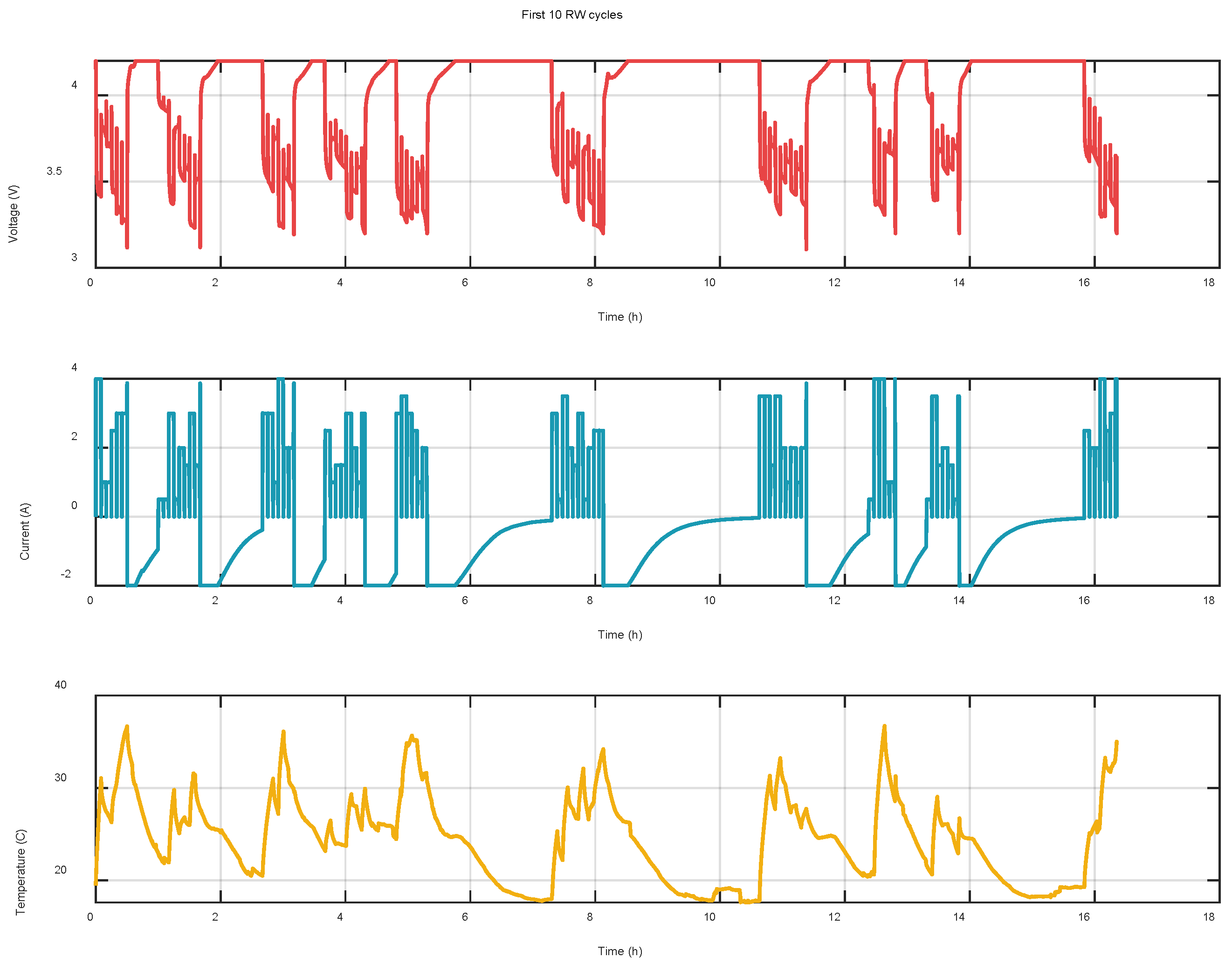
Figure 2.
Reference discharge profiles are segmented into different use cases based on the ranges defined in Table 3. Background colors represent different use cases, and the color gradient of the curves illustrates the evolution of profiles with increasing RW cycles.
Figure 2.
Reference discharge profiles are segmented into different use cases based on the ranges defined in Table 3. Background colors represent different use cases, and the color gradient of the curves illustrates the evolution of profiles with increasing RW cycles.
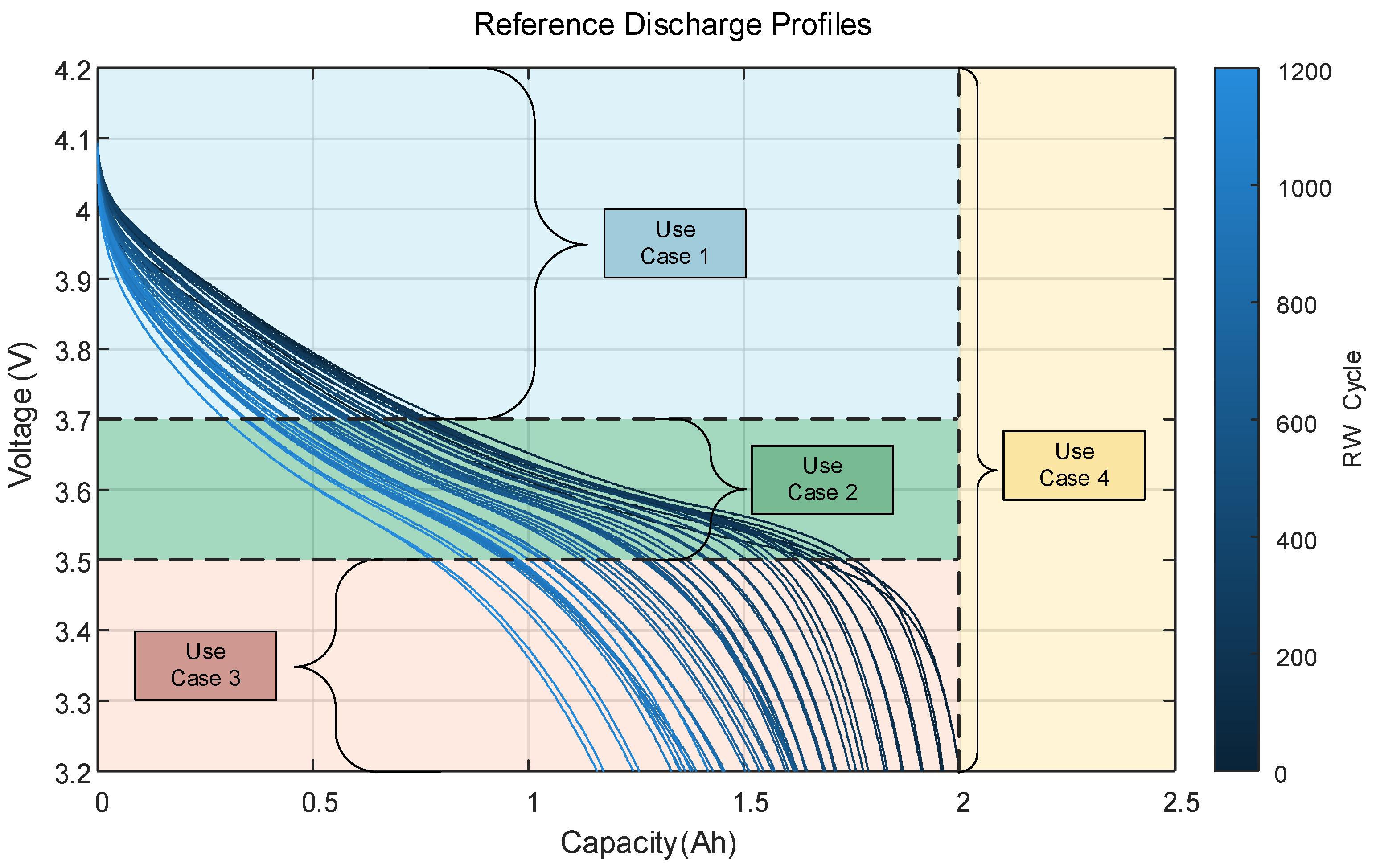
Figure 3.
The structure of basic GAN mode.
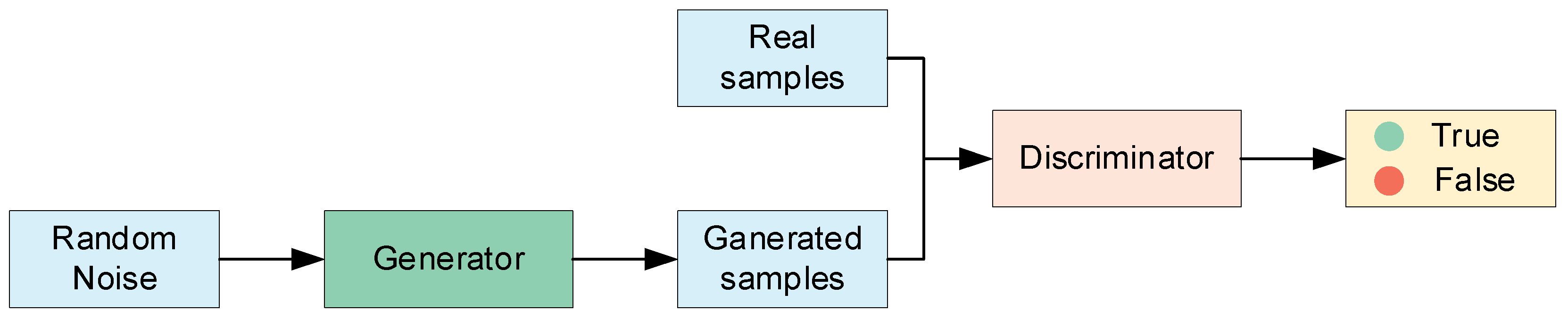
Figure 4.
The overall architecture of DG.
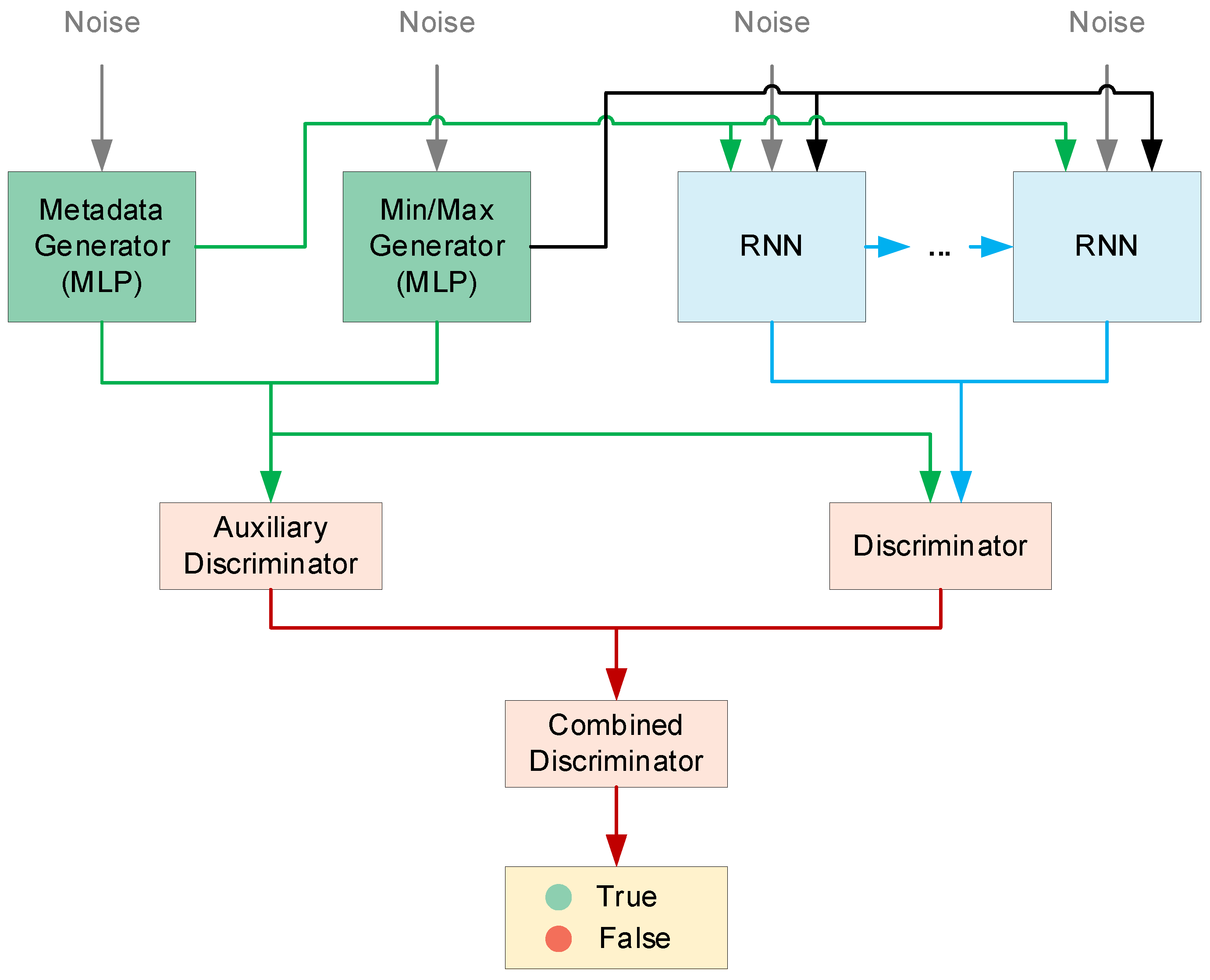
Figure 5.
The overall architecture of TCN.
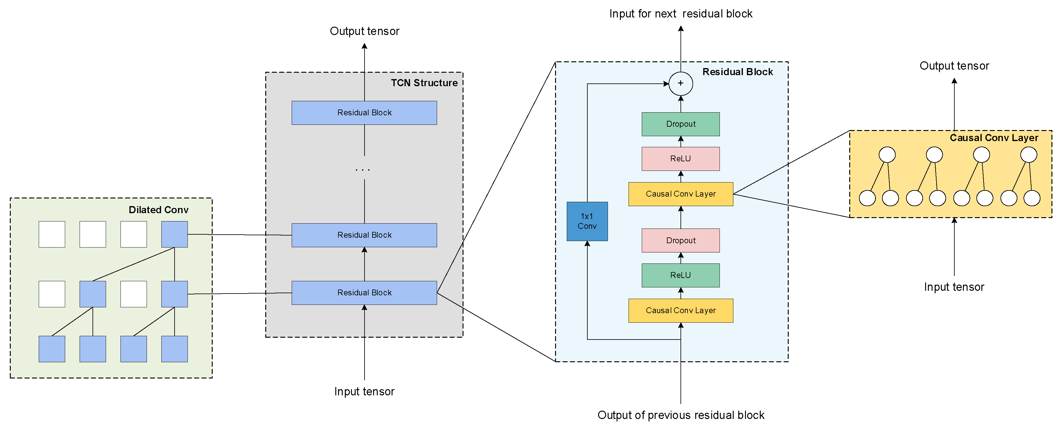
Figure 6.
Causal Convolutional Networks.
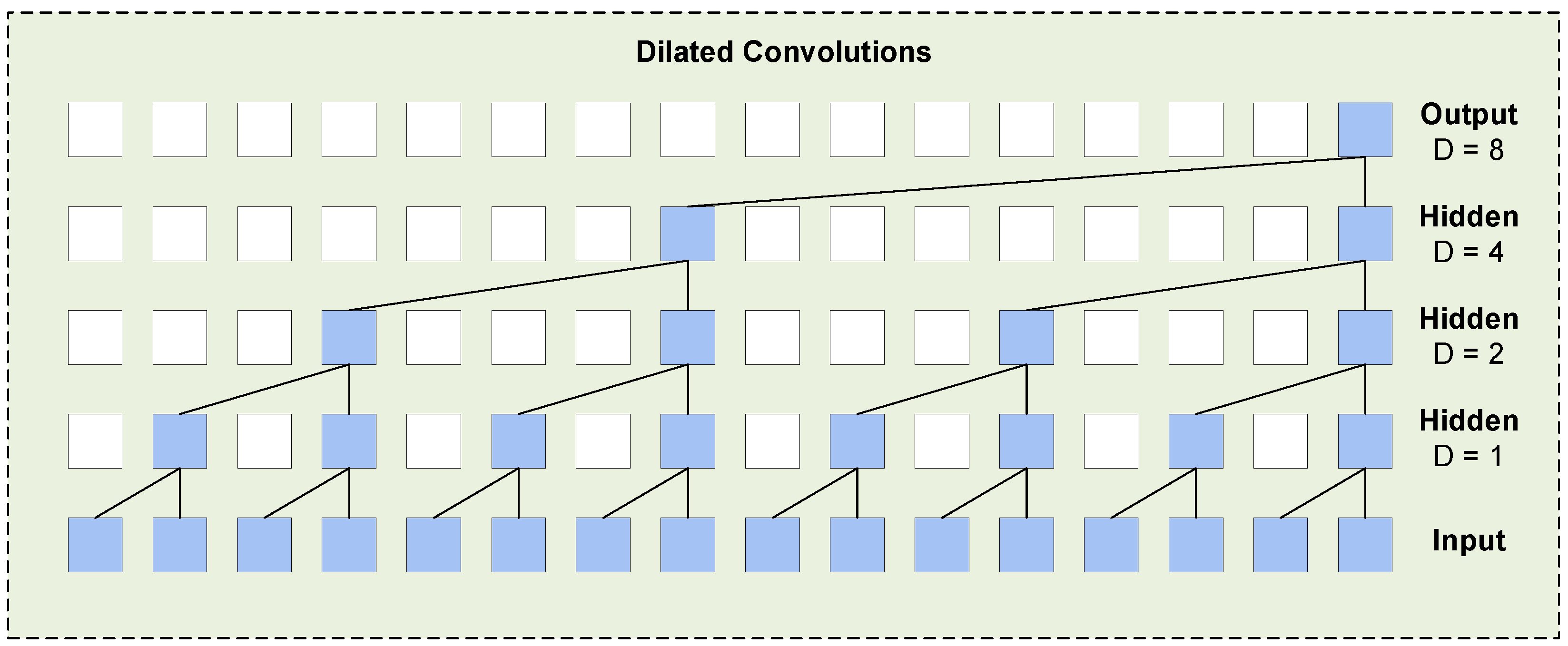
Figure 7.
The overview of the methodology and procedure.
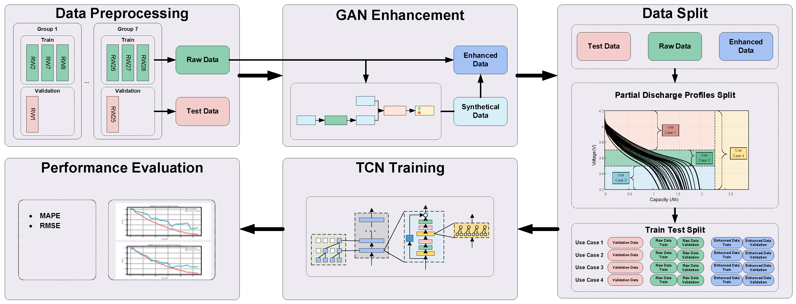
Figure 8.
Original voltage data and synthetic voltage data.
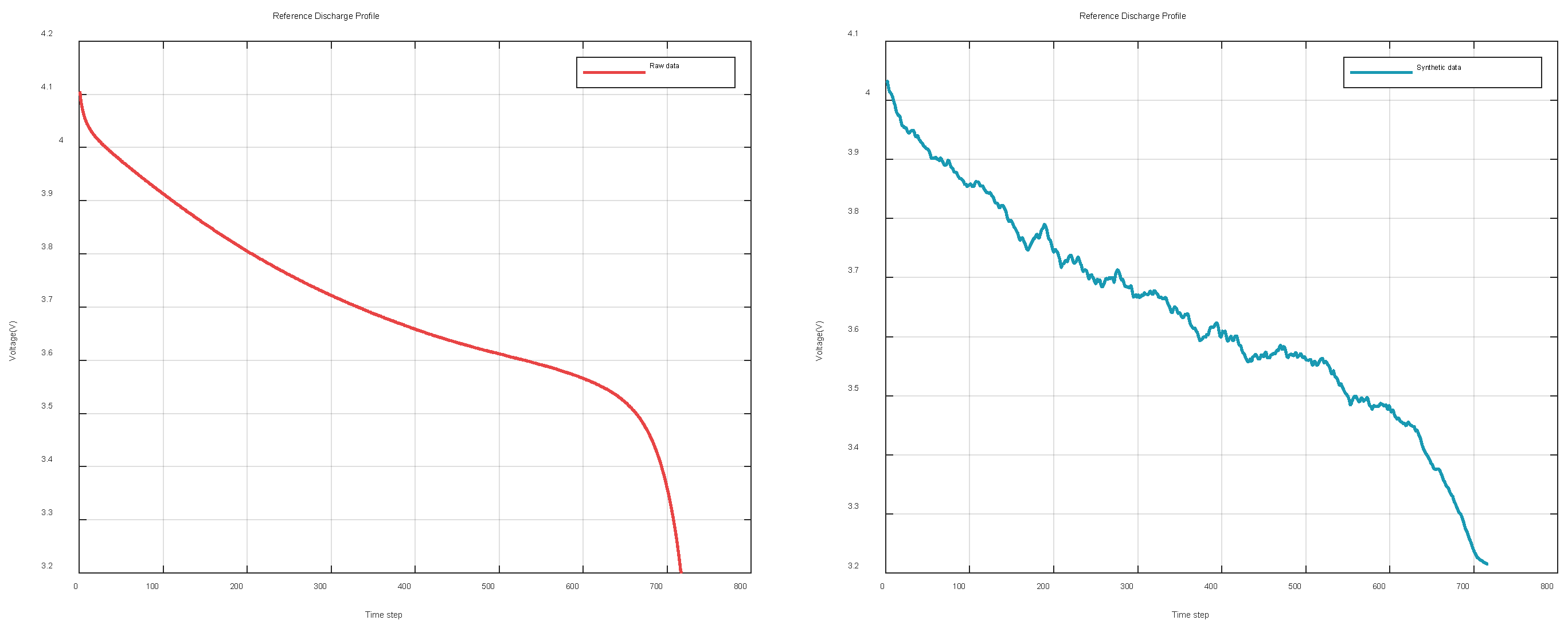
Figure 9.
Original current data and synthetic voltage data.
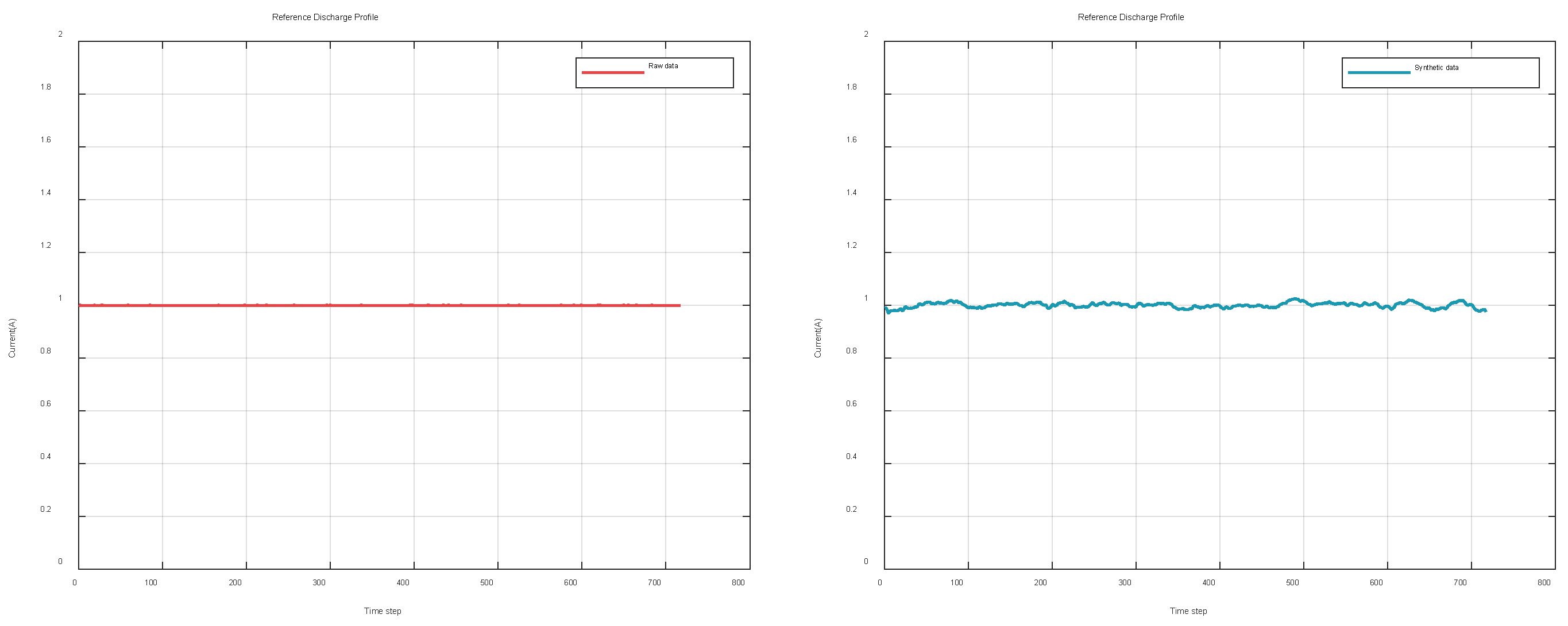
Figure 10.
Visualization of PCA and t-SNE.
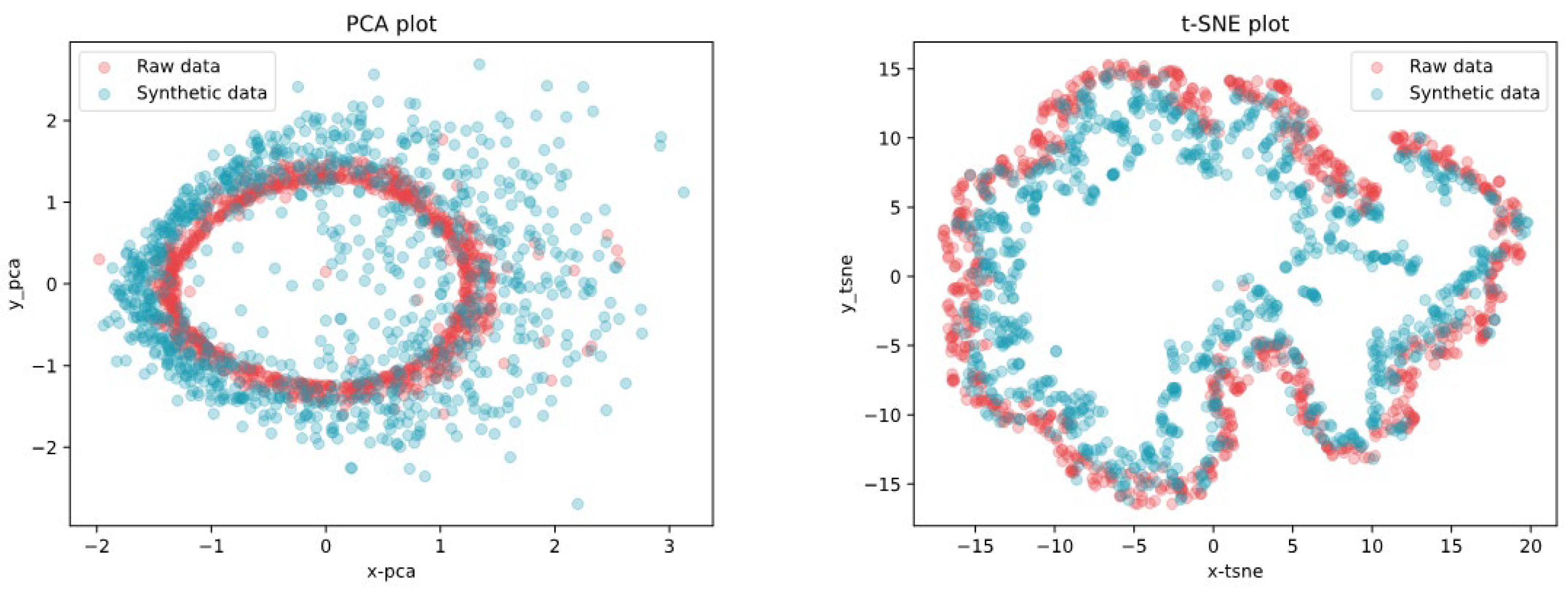
Figure 11.
The experimental results of MAPE.
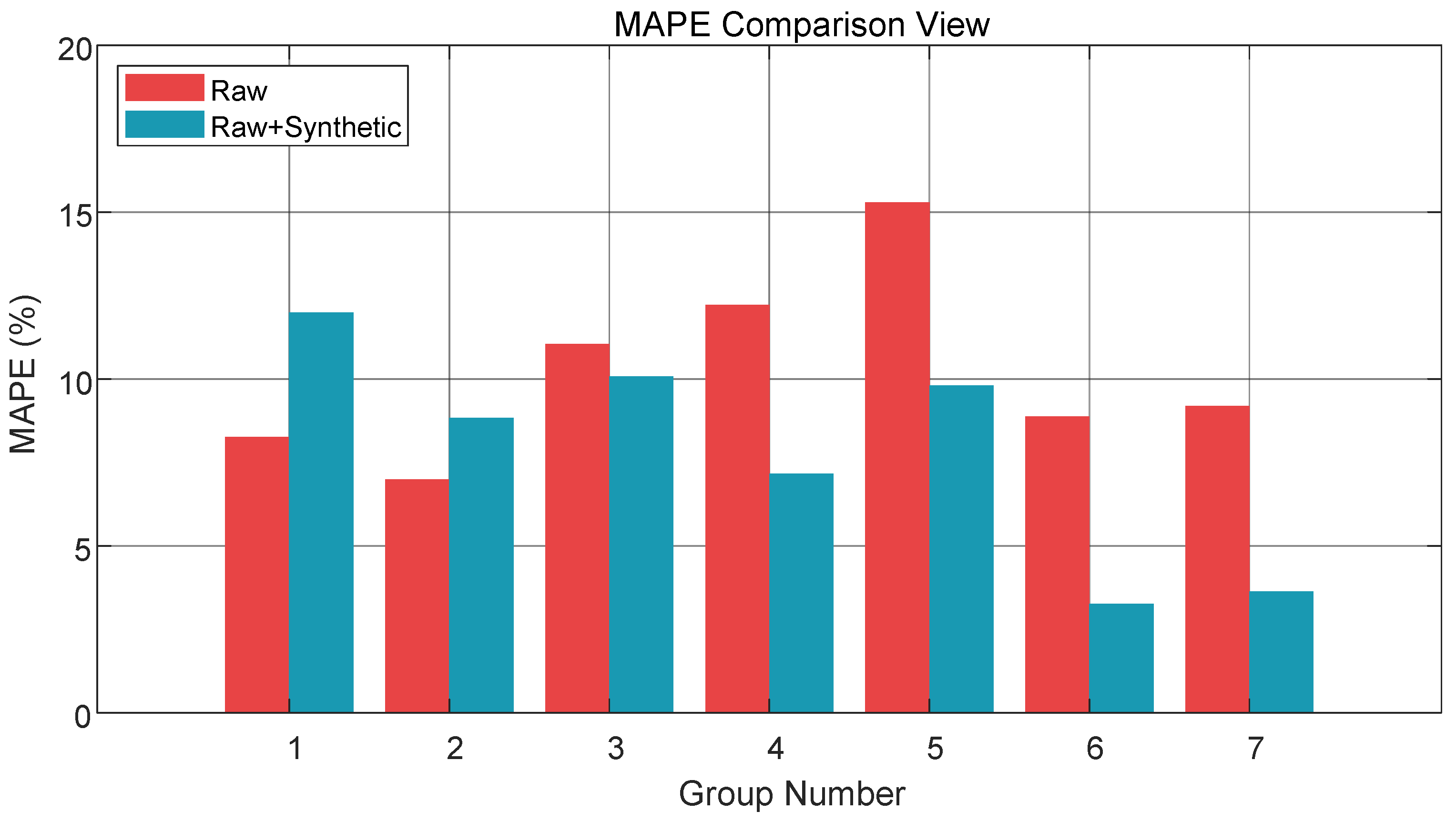
Figure 12.
The experimental results of delta value.
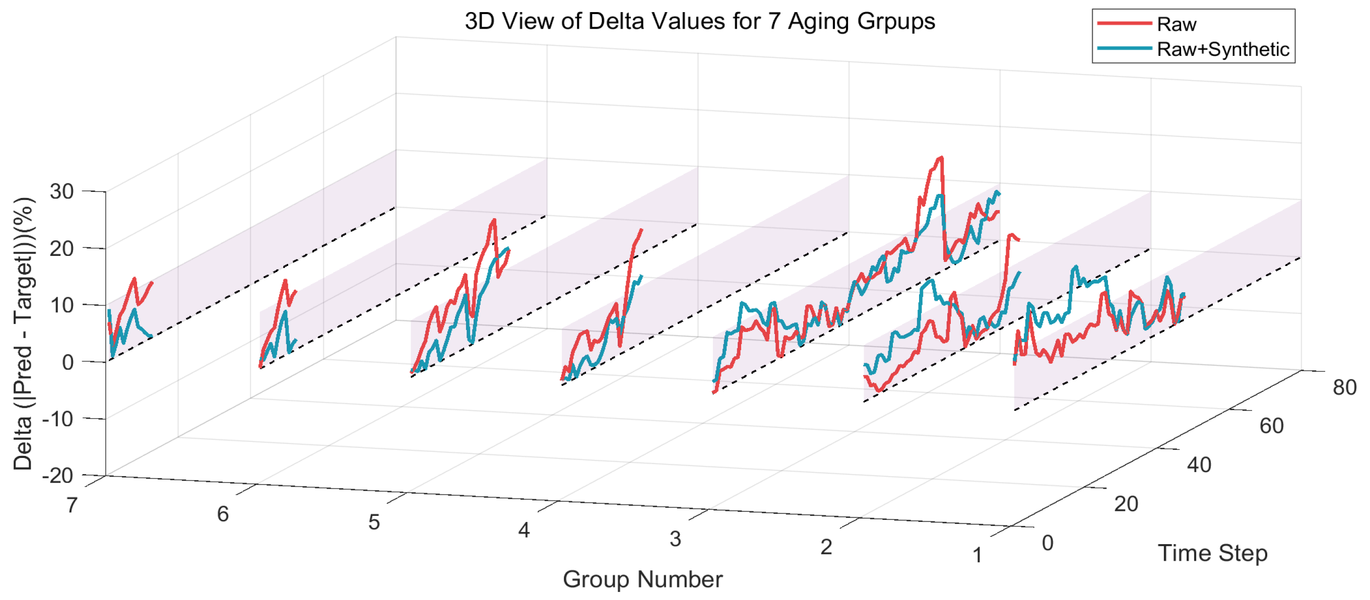

Table 1.
Battery specifications for the NASA PCoE Randomized Battery Usage Data Set.
| Battery Key Characteristics | Specifications |
| Manufacturer | LG Chem |
| Battery chemistry | Lithium cobalt oxide vs. graphite |
| Nominal capacity | 2.1Ah |
| Lower cut-off voltage | 3.2 V |
| Upper threshold voltage | 4.2 V |
Table 2.
NASA PCoE Randomized Battery Usage Data Set test conditions and groups.
| Group(Cells Id) | Test Conditions |
|
Group 1 (RW1,RW2.RW7,RW8) |
Randomized charging (0.5–3 h) to 4.2 V and discharging to 3.2 V with currents between -0.5 A and -4 A. Reference tests every 50 cycles. |
|
Group 2 (RW3-RW6) |
Non-randomized charging to 4.2 V and discharging to 3.2 V with randomized currents (-0.5 A to -4 A). Reference tests every 50 cycles. |
|
Group 3 (RW9-RW12) |
Charging and discharging with randomized current pulses (30 min–3 h). Discharging currents between -0.5 A and -4 A. Reference tests every 1500 cycles. |
|
Group 4 (RW13-RW16) |
Charging to 4.2 V and discharging to 3.2 V with customized probability distribution (peak at 4 A). Load points are updated every minute. Tests at ~40 °C. Reference tests every 50 cycles. |
|
Group 5 (RW17-RW20) |
Same as Group 4, but the ambient temperature was not strictly controlled (lower than 40 °C). Reference tests every 50 cycles. |
|
Group 6 (RW21-RW24) |
Same as Group 4, but the probability distribution skewed toward lower currents (peak at 2 A). Tests at ~40 °C. Reference tests every 50 cycles. |
|
Group 7 (RW25-RW28) |
Same as Group 6, but the ambient temperature was not strictly controlled (lower than 40 °C). Reference tests every 50 cycles. |
Table 3.
SOC ranges and voltage ranges to fragment the partial discharge profiles.
| Use case | SOC ranges | Voltage ranges |
| 1 | 100% to 66.7% | 4.2V to 3.7V |
| 2 | 66.7% to 33.3% | 3.7V to 3.5V |
| 3 | 33.3% to 0% | 3.5V to 3.2V |
| 4 | 100% to 0% | 4.2V to 3.2V |
Table 4.
The hyperparameters of the DG model.
| Hyperparameters | Values |
| max_sequence_len | 700 |
| sample_len | 500 |
| batch_size | 1000 |
| generator_learning_rate | 1e-4 |
| discriminator_learning_rate | 1e-4 |
| epochs | 5000 |
Table 5.
The hyperparameters of the TCN model.
| Hyperparameters | Values |
| input_size | 1 |
| output_size | 1 |
| kernel_size | 3 |
| dropout | 0.33 |
| Dilation | [1, 2, 4, 8, 16, 32, 64] |
| earning_rate | 0.001 |
| epochs | 5000 |
Table 6.
The experimental results of MAPE and RMSE.
| Group | Raw data | Raw+ Synthetic data | ||
| MAPE | RMSE | MAPE | RMSE | |
| 1 | 8.2710% | 0.0749 | 11.9831% | 0.1121 |
| 2 | 6.9889% | 0.0624 | 8.8346% | 0.0772 |
| 3 | 11.0467% | 0.0745 | 10.0822% | 0.0684 |
| 4 | 12.2142% | 0.0936 | 7.1604% | 0.0571 |
| 5 | 15.2889% | 0.1065 | 9.8016% | 0.0741 |
| 6 | 8.8731% | 0.0825 | 3.2651% | 0.0359 |
| 7 | 9.1879% | 0.0819 | 3.6310% | 0.0409 |
Disclaimer/Publisher’s Note: The statements, opinions and data contained in all publications are solely those of the individual author(s) and contributor(s) and not of MDPI and/or the editor(s). MDPI and/or the editor(s) disclaim responsibility for any injury to people or property resulting from any ideas, methods, instructions or products referred to in the content. |
© 2025 by the authors. Licensee MDPI, Basel, Switzerland. This article is an open access article distributed under the terms and conditions of the Creative Commons Attribution (CC BY) license (http://creativecommons.org/licenses/by/4.0/).
Copyright: This open access article is published under a Creative Commons CC BY 4.0 license, which permit the free download, distribution, and reuse, provided that the author and preprint are cited in any reuse.


