Submitted:
21 February 2025
Posted:
24 February 2025
You are already at the latest version
Abstract
During the intense heatwaves of late summer 2024, Washington, DC’s urban landscape revealed the powerful influence of urban morphology on microclimates and air quality. This study investigates how building height-to-width (H/W) ratios impact the urban heat island (UHI) effect, using a combination of field measurements and CFD simulations to understand the dynamics. Street-level data collected from late August to November 2024 across three sites in Washington DC. show that high H/W ratios 2.5–3.0, significantly increased temperatures 30.12–32.10°C and reduced wind speeds 0.02–3.20 m/s, leading to elevated pollutant concentrations, with PM2.5 averaging 2.19 µg/m³. Meanwhile, lower H/W ratios less than 1.5 demonstrated better air circulation and lower pollution levels. The CFD simulations are in good agreement with the experimental data yielding an RMSE of 0.75 for temperature, thus demonstrating its utility for forecasting UHI effects under varying urban layouts. These results demonstrate the potential of CFD in not only modeling but also predicting UHI dynamics, providing valuable tools for urban planners to mitigate heat and improve air quality through strategic design decisions.
Keywords:
Urban Heat Island (UHI)
; Urban microclimate (UMC)
; Urban morphology
; Air Quality
; Temperature distribution
; Wind speed
; Computational Fluid Dynamics (CFD)
; ENVI-met
; Mobile monitoring
; Sensor nodes
1. Introduction
The Urban Heat Island (UHI) phenomenon occurs when urban areas exhibit higher temperatures than their rural surroundings, with temperature differences ranging from 1 ° C to 7 ° C [1,2]. This phenomenon arises from a combination of factors, including the absorption and retention of heat by urban infrastructure, anthropogenic heat release, and reduced vegetative cover [3,4]. UHI increases air pollution through the elevated formation of tropospheric ozone and particulate matter, and disrupts urban thermal dynamics, influencing wind flow and pollutant dispersion [5,6] .
Urban microclimates, influenced by localized climatic conditions, amplify the challenges posed by UHI. These include heat retention, reduced nighttime cooling, and entrapment of pollutants in street canyons [7,8]. For example, elevated temperatures induced by UHI accelerate chemical reactions that increase nitrogen oxide (NOx) emissions by up to 25% and tropospheric ozone concentrations by 15% during heat events.
To study the complexity of the interaction between Urban Heat Island (UHI) and urban microclimates, researchers have adopted diverse measurement methods, each with unique advantages and limitations. Traditional meteorological stations, such as those of Santamouris to analyze urban heat islands in Europe, provide long-term reliable data but often lack the spatial resolution needed to capture detailed urban variability effectively [9]. Similarly, Yang et al. used network of weather stations to explore urban microclimates, highlighting their utility but also their limitations in representing spatial heterogeneity [10]. Remote sensing techniques, particularly satellite-based Land Surface Temperature (LST) data, offer valuable large-scale insights. For example, the Moderate Resolution Imaging Spectroradiometer (MODIS) and Landsat have been extensively used to monitor urban microclimates due to their high spatial resolution [11,12]. However, these methods require complementary in situ data to validate findings and address low temporal resolution [12]. Mobile monitoring sensing tools, including wearable devices and vehicle-based platforms, provide a finer spatial understanding of microclimatic variations.
Numerical models, such as Computational Fluid Dynamics (CFD), complement observational techniques by simulating urban airflow, pollutant dispersion, and temperature patterns. For example, Reynolds-average Navier-Stokes (RANS) models have been widely used for their computational efficiency in simulating mean flow fields [7], while Large Eddy Simulations (LES) provide a detailed understanding of the dynamics of turbulence in urban environments [13].
Air quality monitoring has significantly improved, starting with stationary monitoring stations that provided long-term pollutant data monitoring. But these stations often lacked spatial coverage, and mobile platforms, such as vehicle-based systems and portable sensors, have become essential to capture fine-scale variations in air quality. The introduction of low-cost sensors and mobile networks has greatly improved spatial density, complemented meteorological data and providing real-time pollutant measurements [9,10]. For the past decade, air quality monitoring has been integrated with numerical models, such as Computational Fluid Dynamics (CFD), to simulate pollutant dispersion and interactions with temperature and urban structures [12].
Limited budgets often constrain investments in high-end measuring instruments, making low-cost monitoring systems essential, particularly in low- and middle-income countries. These regions can benefit from alternative technologies, such as citizen-built monitoring devices, which leverage open hardware platforms such as Sensor.Commumity and PurpleAir [7,14]. However, the widespread adoption of these systems raises concerns regarding data accuracy and reliability. To ensure the validity of the measurements, low-cost sensors need proper calibration against reference instruments or well-established standards [15].
There are two approaches for calibration: maximizers, who require high-end equipment and state-of-the-art methods like co-location experiments, and satisficers, who focus on achieving adequate reliability within a budget. Satisficers improve data quality by using cost-effective calibration methods, such as manipulating temperature and humidity with Peltier coolers, heaters, or saturated salt solutions [14,15,16,17,18,19,20,21,22,23,24] . For gas sensors, controlled gas introduction via disposable syringes is used.
This study focuses on Washington, DC, during late summer to early fall 2024, employing mobile sensing techniques to investigate the spatial variability of UHI effects across diverse urban morphologies. By analyzing temperature, wind speed, and pollutant concentrations, the research aims to elucidate the intricate relationships between UHI, urban microclimates, and environmental challenges in complex urban settings [25,26].
2. Materials and Methods
2.1. Experimental Setup
Figure 1 shows the experimental sites under investigation for microclimatic measurements from August to November: Veazey Street NW (38°56′39.75″N, 77°3′51.50″W), Connecticut Avenue NW (38°56′51.82″N, 77°3′54.69″W), and Van Ness Street NW (38°56′51.82″N, 77°3′54.69″W). Figure 1a. shows Veazey Street NW is located near the city’s residential core and features low-rise buildings with a height of 10-15 meters and street widths ranging from 15-20 meters, giving it an H/W ratio of 0.5-0.75. Figure 1b. shows Connecticut Avenue NW (38°56′51.82″N, 77°3′54.69″W), with taller buildings (20-30 meters) and a street width of 10-15 meters, has a higher H/W ratio of 1.5-2.0. The dense traffic, both vehicle and pedestrian, along with the compact street design, creates unique microclimatic conditions, leading to temperature shifts and altered wind patterns. Figure 1c shows Van Ness Street NW (38°56′51.82″N, 77°3′54.69″W) features buildings between 6-10 meters in height, and street widths 20-25 meters, with an H/W ratio of 0.3-0.5. This primarily residential area allows for better air circulation compared to the other two streets but still experiences notable pollutant levels due to its traffic.
2.2. Sensor Nodes
The experiment utilized a range of environmental sensors to monitor urban microclimates, with nodes placed at different locations to measure key parameters summarized in Table 1. The sensors included the PMS5003 for particulate matter (PM1.0 to PM10), the MICS 6814 for gases such as CO, NO2, and NH3, and the SEN0385 for ambient temperature and humidity. Additionally, an ultrasonic wind sensor measured wind speed and direction. Table 1 summarizes the sensors used with their measured parameters, accuracy, and resolution.These sensors were integrated into environmental nodes that were deployed across sites, with each node collecting real-time data for later analysis.
The process of building the sensor nodes began by organizing sensors into two groups based on power requirements and functionality as depicted in Figure 2. High-power sensors, such as the DFRobot Multigas sensor O3 DFRobot Temperature and Humidity Sensor (SEN0385) , were placed in one group, while low-power sensors, including the PMS5003 (particulate matter) and MICS-6814 (CO, NO2, NH3), were placed in another. This approach helped evaluate each node’s performance while optimizing power consumption between 3.3V and 5V. Lithium batteries, with a capacity of 40 mAh and a runtime of 8–10 hours, powered the system. The first node (Figure 2a) consisted of the PMS5003 and MICS-6814 sensors, while the second node (Figure 2b) included the DFRobot temperature and humidity sensor and the DFRobot Gas Sensor for ozone (O3). This setup ensured efficient operation and effective testing of each node.
2.2.1. Hardware Description
The data collection system was developed using the Arduino Integrated Development Environment (IDE) version 1.8.19. This software platform, based on the C/C++ programming language, retains key functionalities from earlier versions of the IDE. The overall process involves the initialization of hardware components, sensor validation, and data storage [27] . Initially, the Arduino hardware is set up, with pins defined for communication with the sensors, and checks are made to ensure their functionality. Sensor validation follows, with digital sensors reporting immediately and analog sensors requiring stabilization. The data collection process is cyclic, with measurements taken, validated, and anomalous data flagged or discarded. The data is then stored in a CSV format, compatible with MATLAB and MS Excel for analysis, and transmitted via the ESP-01 Wi-Fi module. Connectivity is monitored, ensuring reliable data storage on the SD card. Finally, sensor calibration experiments are conducted, and the system is deployed for real-world data collection. Figure 3 depicts the flowchart diagram of Arduino Uno process for collecting data from the sensor nodes.
2.2.2. Software Description
The software monitoring interface for the provided Arduino code is designed to collect and display data from multiple environmental sensors, including air quality sensors (NO2, NH3, CO, O3) and a temperature-humidity sensor (SHT3x), while also saving the results to an SD card.
2.2.3. Sensor Calibration Methods
The calibration of the SEN0385 temperature sensor was conducted by comparing its readings with the ambient temperature provided by the Ultrasonic Portable Solar Instrument (Calypso), which acted as the reference. The Calypso, known for its high accuracy (±0.1°C), was used as the "golden standard" for temperature measurements. It also accounted for environmental factors such as humidity, wind speed, and direction, which enhanced the accuracy of the temperature readings. Data from both the SEN0385 and the Calypso Instruments were analyzed, and a calibration curve was created. This curve enabled adjustments to the SEN0385 sensor, ensuring its future temperature measurements are accurate, consistent, and reliable.
Similarly, the calibration of the DFRobot SEN0472 Ozone (O3) sensor was performed in an indoor, typically clean environment (see Figure 4) to ensure accurate ozone measurements. The sensor was first installed and allowed to warm up for stabilization. In clean ambient air, baseline readings were recorded to establish background ozone levels, typically ranging from 0 to 0.1 ppm. A calibration curve was then developed to correct sensor deviations, ensuring reliable future ozone measurements.
The calibration process for the MICS-6814 gas sensor (for CO and NO2) and the PMS5003 particulate matter sensor followed the same procedure used for the SEN0472 ozone sensor. Both sensors were calibrated in an indoor, clean environment. Baseline readings were recorded, and known concentrations of gases and particulate matter were introduced to the sensors. Calibration curves were developed to adjust for sensor deviations, ensuring their future measurements are accurate and reliable.
2.3. UHI Index
The Urban Heat Island (UHI) index is a key measure used to assess the temperature difference between urban areas and their surrounding rural environments. It is commonly defined as the difference in temperature between the land surface temperature (LST) of an urban area and that of a rural or suburban area. The UHI index can also be expressed in air temperature between the two areas, reflecting the heat retention and generation within urban environments compared to less developed, rural settings. The basic formula for the UHI index is:
where represents the temperature of the urban area and is the temperature of the surrounding rural area, both expressed in degrees Celsius (°C) or Kelvin (K). This index is vital for understanding the extent of the UHI effect, as urban areas tend to retain heat due to increased surface roughness, building materials, and human activities, leading to higher temperatures compared to rural areas [28]. To quantify Urban Heat Island (UHI) effects, temperature and wind data from Germantown, Maryland, a suburban reference site, were used as a baseline for comparison. This data, obtained from the Open-Meteo Historical Weather (Open-Meteo, n.d.), represented atmospheric conditions with lower urban influence. This comparison with suburban data provided a means to isolate urban-induced thermal and air quality anomalies.
2.4. Numerical Analysis
To numerically assess the correlation between local microclimate and specific constrains of the area, the numerical model was developed using some measurement data. For thermal comfort evaluation, the Predicted Mean Vote (PMV) index was used, as it considers factors such as air temperature, humidity, wind speed, and clothing, providing a quantitative assessment of thermal comfort [29]. The model was calibrated and validated with real-world data to ensure accuracy.
2.4.1. Computational Fluid Dynamics (CFD) Microclimate Modeling
ENVI-met LITE version 5.7.1 was selected due to its ability to accurately resolve environmental variations within the urban canopy layer using a three-dimensional computation fluid dynamics (CFD) approach. The software employs the orthogonal Arakawa C-grid for numerical discretization, which allows fine spatial resolution and incorporates complex topographical and urban features. ENVI-met uses Reynolds-averaged Navier-Strokes (RANS) equations to calculate the wind field, incorporating the Bruse/ENVI-met 2017 Turbulence Kinetic Energy (TKE) model to account for energy distribution and dissipation in the air. The surface temperatures of fades were calculated using a three-node transient state model, and the finite difference method was employed to solve partial differential equations within the system.
Figure 5 shows the aerial of the Veazey St. NW experimental site and illustrates the realistic model of this urban heat area, developed and calibrated using the data collected in the first set of experiments. The calibration and validation process were performed according to the AHRAE Guideline 14(ANSI/ASHRAE, 2023) using the data obtained from the environmental and air quality sensors. The model was further refined by incorporating building materials that most closely matched those found at the experimental site. Specifically, the wall materials were modeled with moderate insulation. These simulations allowed for an accurate representation of the UHI effects, including temperature and wind dynamics, and provided an understanding of the interaction between the built environment and atmospheric conditions.
The blueprint model simulations revealed that temperature and wind speed vary with respect to building orientation and height, width between the building surfaces, and wind direction. High elevation buildings are more likely to trap and retain heat than low elevation buildings. Also, narrow street canyons are more likely to experience lower wind speeds than wider street canyons experience. Figure 6 highlights the temperature variation and wind speed, where the highest temperatures were recorded between buildings with the largest H/W ratios (1.5 and 1.2), where temperatures reached 18.2°C and 16.73°C, respectively. These areas also experienced the lowest wind speeds, ranging from 0.11 to 0.49 m/s. On the other hand, a building with a smaller H/W ratio of 0.28 resulted in a lower temperature of 15.5°C, but with significantly higher wind speeds of 6.07 m/s.
2.4.2. Height-to-Width(H/W) Ratio Analysis
The study also investigated the influence of the height-to-width (H/W) ratio on the microclimatic variability across the experimental sites. The H/W ratio is a critical parameter in urban morphology, as it determines the extent of solar radiation, wind flow, and heat retention within urban canyons [29-31]. Table 2 2 summarizes the H/W ratio of each experimental site calculated based on the building heights and the width of the streets.
The thermo-physical properties of the materials presented in Table were determined based on a combination of literature reviews and commonly accepted data from various sources. The values for walls with moderate insulation were derived from standard construction materials and insulation types commonly used in building design, as found in studies like those by Pisello et al. and similar research. Asphalt roof and roofing tile properties were sourced from industry-standard material data sheets and studies on building materials’ thermal performance. For greenery, the values were obtained from research on vegetation and its thermal properties, particularly focusing on its role in urban microclimates and heat island mitigation. These values serve as approximations for the materials’ behavior in thermal simulations, ensuring a realistic representation of their performance in urban settings.
2.5. Thermal Comfort Index
The study incorporated a thermal comfort index analysis using Predicted Mean Vote (PMV) model and the Physiological Equivalent Temperature (PET) as key parameters. The PMV index, developed by Fanger , integrates environmental and physiological factors such as air temperature, humidity [29] , wind speed, clothing insulation, and metabolic activity. It is typically calculated using a detailed formula that considers the balance between heat produced by the body and heat lost to the environment.
The PET index, developed by Höppe , is derived using the Munich Energy Balance Model for individuals (MEMI) and represents air temperature at which the human body maintains heat balance. PET accounts for parameters such as solar radiation, wind speed, humidity, and the thermal resistance of clothing and is usually expressed in degrees Celsius [30].
In this study, simulations for both PMV and PET were conducted using an average female subject with summer clothing (clothing insulation of 0.5 clo) and a metabolic activity of 1.2 met. These indices were applied to assess the thermal comfort of individuals at each experimental site and evaluate the impacts of UHI on residents’ comfort. They also provided critical insights into the correlation between UHI intensity and thermal comfort, supporting microclimate analysis [28,29].
2.6. Data Calibration
To evaluate of the numerical model the following calibration indexes are evaluated [31]:
- Root Mean Square Error (RMSE): Represents the average magnitude of errors between sensor readings and reference (simulation) values. It is expressed as:where denotes the reference value, is the corresponding sensor reading, and n is the total number of observations. A smaller RMSE indicates better accuracy.
- Correlation Coefficient (): Quantifies the linear relationship between sensor readings and simulation measurements. It is calculated as:where is the mean of the reference values. An value close to 1 indicates a strong positive correlation, meaning the sensor data follows the trends of the simulation results.
3. Results
3.1. Sensor Data Calibration
The SEN0385 temperature sensor and the ozone sensor both exhibited lower readings compared to their respective reference instruments, with temperature differences ranging from 0.01 °C to 0.3 °C and ozone variations between 0.01 ppm and 0.02 ppm. Similarly, the MICS 6814 sensor (NO2 and CO) showed discrepancies between reference values. For NO2 raw readings ranged from 1.92 to 2.42 ppm, while the reference values ranged from 1.94 ppm to 2.45 ppm. The CO raw readings ranged from 1.97 ppm to 2.19 ppm, with the reference values ranging from 1.99 to 2.21 ppm. To correct these biases, a linear model was applied:
The slopes (1.023 for temperature, 1.05 for ozone, 0.95 for NO2, and 0.98 for CO) indicate that for every 1-unit increase in raw sensor readings, the adjusted values increase proportionally, while the intercepts account for minor offsets. Figure 7, Figure 8 and Figure 9 highlight these differences for each sensor, with dashed lines representing the calibration models and the adjusted sensors data after applying corrections.
3.2. UHI Microclimate: Urban Morphology
The relationship between temperature and Height-to-Width (H/W) ratio across the three monitored locations—Veazey St. NW, Connecticut Ave. NW, and Van Ness St. NW—shows a clear correlation between urban morphology and thermal conditions. Figure 10 illustrates temperature variations from November 6th to November 7th (9 PM- 3PM) at the three locations, with each site characterized by a distinct H/W ratio. Connecticut Ave. NW, with the lowest H/W ratio (1.5–2.0), consistently exhibited the highest temperatures, reaching up to 24.96°C during the evening of November 6, 2024. The wide street layout and minimal shading amplify solar exposure, resulting in elevated thermal conditions. Conversely, Van Ness St. NW, which has the highest H/W ratio (0.3–0.5), recorded the lowest temperatures throughout the monitoring period, with values dropping to 18.08°C during the early hours of November 7, 2024. Veazey St. NW, with a moderate H/W ratio (0.5–0.75), exhibited intermediate temperature values, ranging between those of Connecticut Ave. NW and Van Ness St. NW. On average, the temperature at Veazey St. NW was 1.5°C lower than Connecticut Ave. NW but 0.5°C higher than Van Ness St. NW.
3.2.1. UHI Microclimate parameters: Temperature and Wind Speed
Figure 11 shows that on August 26th , data between the hours of 3pm and 4pm the recorded peak temperatures were 32 and 31 Celsius in DC and Germantown, respectively. The recorded temperature in August was consistently higher in DC than Germantown. Additionally, peak wind speeds were 4.7 m/s and 2.7 m/s in DC (at 1pm) and Germantown (at 6:30 pm), respectively. In the afternoon and evening hours, the recorded wind speeds were consistently much higher in DC than Germantown. On October 4th, between the hours of 3pm and 4pm, the recorded peak temperatures were 24°C in DC and 23°C in Germantown. Throughout the day, temperatures were consistently higher in DC compared to Germantown. Additionally, peak wind speeds reached 3.9 m/s in DC (at 1pm) and 2.5 m/s in Germantown (at 6:30pm). During the afternoon and evening hours, wind speeds in DC were consistently much higher than in Germantown. On November 6th, between 9:00 pm and 11:00 pm, temperatures ranged from 20.4°C to 17.7°C in Germantown and from 23.61°C to 20.33°C at Veazey St NW. Wind speeds in Germantown ranged from 1.55 m/s to 2.21 m/s, while at Veazey St NW, they ranged from 3.12 m/s to 3.07 m/s. On November 7th, temperatures in Germantown ranged from 16.8°C at 6:00 am to 23.8°C at 12:00 pm. At Veazey St NW, temperatures ranged from 18.69°C to 24.11°C. Wind speeds in Germantown ranged from 1.57 m/s to 4.5 m/s, with the highest at 1:00 pm. At Veazey St NW, wind speeds ranged from 1.68 m/s to 3.85 m/s. During the afternoon, wind speeds were higher in Germantown compared to Veazey St NW.
3.2.2. UHI Microclimate Parameters and Pollutant Concentration
Figure 12 illustrates the correlation between temperature and the concentrations of Ozone (O3), Nitrogen Dioxide (NO2), Carbon Monoxide (CO), and PM2.5 on August 26, 2024. The temperature ranged from 24.4°C to 31.1°C, peaking in the afternoon and cooling towards the evening. O3 concentrations fluctuated between 0.2 ppm and 0.4 ppm, showing a weak positive correlation with temperature. NO2 concentrations ranged from 2.06 ppm to 2.48 ppm, with a moderate positive correlation to temperature, peaking in the afternoon as temperatures increased. CO levels remained relatively stable between 2.22 ppm and 2.33 ppm, showing a weak correlation with temperature. PM2.5 concentrations were stable at around 2.8 µg/m³, with little variation and no significant correlation to temperature. The correlation analysis for August 26th showed that O3 had a weak positive correlation (r = 0.13), NO2 had a moderate positive correlation (r = 0.71), CO had a weak positive correlation (r = 0.27), and PM2.5 had no correlation (r = 0.09) with temperature. Figure 14b displays the correlation between temperature and the concentrations of Ozone (O3), Nitrogen Dioxide (NO2), Carbon Monoxide (CO), and PM2.5 in the late afternoon and evening. The temperature ranged from 19.4°C to 24°C, gradually decreasing as evening approached. O3 concentrations remained stable at 0.2 ppm initially and then decreased to 0.1 ppm, showing a very weak negative correlation with temperature. NO2 concentrations ranged from 1.92 ppm to 2.42 ppm, with a weak negative correlation to temperature. CO levels fluctuated between 2.16 ppm and 2.19 ppm, showing no significant relationship to temperature. PM2.5 concentrations remained constant at 0.4 µg/m³, with no correlation to temperature. Correlation analysis for October 04, 2024, revealed that O3 had a very weak negative correlation (r = -0.12), NO2 had a weak negative correlation (r = -0.45), CO had no correlation (r = -0.09), and PM2.5 had no correlation (r = 0.00) with temperature.
3.3. Numerical Analysis
On August 26, 2024, simulations indicated high air temperatures, low wind speeds, and considerable thermal discomfort in the study area, particularly in areas between buildings with limited airflow. In contrast, the evening and early morning hours of November 6-7, 2024, exhibited significantly cooler temperatures, greater wind variability, and more favorable thermal conditions. Figure 15 illustrates the temperature distribution for both days. On August 26, temperatures ranged from 30.38°C to 32.29°C, with the highest values occurring around the airflow-restricted zones between buildings . In contrast, temperatures on November 6-7 were lower, peaking at 19.45°C, reflecting cooler conditions during the evening and early morning hours (see Figure 13 and Figure 14 presents the wind speed variations for both dates. On August 26, wind speeds ranged from 0.03 m/s to 3.50 m/s, indicating calm conditions that hindered natural cooling. During the November 6-7 period, wind speeds exhibited greater variation, ranging from 0.01 m/s to 6.07 m/s, showing increased variability and enhanced cooling during the night . Figure 15 shows the PMV values for both days. On August 26, PMV values ranged from 1.97 to 4.74 , suggesting significant discomfort, which could lead to increased sweating and heat accumulation for the average pedestrian due to high temperatures and limited wind flow. Conversely, on November 6-7, PMV values ranged from -1.01 to 1.16, indicating cooler conditions and less heat stress for pedestrians. The PET values ranged from 35°C to 41°C at the simulated experimental site on August 26, signaling that the average pedestrian experienced discomfort due to the higher thermal load. Alternatively, the PET values on November 6-7 ranged from 15°C to 23°C, suggesting more comfortable thermal conditions for the average pedestrian (see Figure 16 .
3.3.1. Data Validation: RMSE, R2
The validation of the experimental and simulated results for air temperature and wind speed shows a strong agreement between the two datasets, as summarized in Table 3. For August 26, the simulated air temperature ranged between 30.12°C and 32.10°C, closely matching the experimental range of 30.38°C to 32.29°C, with an RMSE of 0.75 and an of 0.91. Similarly, the simulated wind speed (0.02–3.20 m/s) aligns well with the experimental values (0.03–3.50 m/s), yielding an RMSE of 0.38 and an of 0.86. During the November 6–7 evening period, the maximum simulated temperature (19.40°C) closely matches the experimental maximum (19.45°C), with an RMSE of 0.62 and an of 0.94, indicating high accuracy. The wind speed comparison for this period also shows good agreement, with simulated values ranging from 0.03 to 4.10 m/s compared to the experimental range of 0.04 to 4.50 m/s, resulting in an RMSE of 0.42 and an of 0.88.
4. Discussion
The results confirm the significant influence of urban morphology on microclimate dynamics, particularly highlighting the role of high height-to-width (H/W) ratios in exacerbating urban heat and air quality challenges. Computational Fluid Dynamics (CFD) simulations, coupled with experimental validation, demonstrated a strong correlation between urban design parameters and microclimatic conditions. For instance, on August 26, simulated air temperatures (30.12°C–32.10°C) closely matched experimental measurements (30.38°C–32.29°C), with an RMSE of 0.75 and a Correlation Coefficient (R²) of 0.91. This high level of agreement underscores the reliability of the CFD model in capturing temperature variations influenced by urban morphology. Similarly, wind speed simulations (0.02–3.20 m/s) were consistent with observed values (0.03–3.50 m/s), yielding an RMSE of 0.38 and an R² of 0.86, further confirming the model’s ability to replicate wind dynamics in urban environments. Comparable accuracy was observed in November, where simulated temperatures (19.10°C–19.40°C) aligned closely with experimental values (19.45°C), achieving an RMSE of 0.62 and an R² of 0.94.
Despite the high accuracy, some discrepancies between simulated and experimental results were attributed to the omission of critical parameters such as Land Surface Temperature (LST), Albedo, and Sky View Factor. These factors are known to influence heat absorption, reflection, and emission, and their exclusion led to minor deviations in the model’s predictions. Addressing these omissions in future studies could further refine the model’s precision.
The findings reveal that areas with higher H/W ratios experienced elevated temperatures, reduced wind speeds, and poorer air quality. During the summer, PM2.5 levels averaged 2.19 µg/m³, and ozone concentrations ranged from 0.2 to 0.3 ppm, indicating significant pollutant accumulation in densely built environments. These results support the hypothesis that compact urban designs, characterized by high H/W ratios, retain heat and restrict ventilation, amplifying the urban heat island (UHI) effect and deteriorating air quality. In contrast, lower H/W ratios were associated with enhanced ventilation and reduced pollutant concentrations, illustrating the importance of urban geometry in mitigating UHI effects.
Additionally, the results highlight the strong influence of urban microclimate variations on thermal comfort, emphasizing the role of urban geometry and ventilation. On August 26, both PMV (1.97–4.74) and PET (35°C–41°C) values indicate severe heat stress, driven by high temperatures, limited airflow, and urban heat retention. This suggests that densely built environments with poor ventilation amplify discomfort, potentially affecting pedestrian well-being and outdoor activity levels. In contrast, the lower PMV (-1.01 to 1.16) and PET (15°C–23°C) values on November 6-7 demonstrate significantly improved comfort due to cooler temperatures and better thermal conditions. The alignment between PMV and PET values underscores their reliability in assessing urban thermal environments.
5. Conclusions
Urban morphology plays a crucial role in shaping microclimate dynamics, with high height-to-width (H/W) ratios shown to increase temperatures, restrict ventilation, and worsen air quality. The strong alignment between CFD simulations and experimental data, evidenced by low RMSE values and high correlation coefficients, demonstrates the effectiveness of modeling techniques in capturing urban thermal and wind dynamics. Compact urban designs with higher H/W ratios were found to intensify the urban heat island (UHI) effect, contributing to elevated pollutant levels due to reduced airflow. Conversely, areas with lower H/W ratios demonstrated improved ventilation and reduced pollutant accumulation, emphasizing the importance of optimizing urban geometry to mitigate UHI effects. The Predicted Mean Vote (PMV) and Physiological Equivalent Temperature (PET) indexes further highlighted the impact of urban design on thermal comfort, reinforcing the need for sustainable planning strategies that prioritize better airflow and reduced thermal stress in urban environments.
Future investigations should prioritize the deployment of pedestrian-level sensing systems to enhance the understanding of urban microclimate variations. These systems, equipped with advanced sensors for real-time monitoring of temperature, humidity, wind speed, and air pollutants such as PM2.5, CO, and NO2, can provide high-resolution data at the human scale. Such localized measurements will allow for better validation of simulation models and a deeper exploration of microclimatic differences influenced by factors like pedestrian activity, traffic, and urban design. Additionally, integrating pedestrian-level data with IoT frameworks and machine learning algorithms could enhance urban climate modeling and support targeted interventions to improve air quality, thermal comfort, and overall urban resilience. This approach offers a promising pathway to developing smarter, healthier, and more adaptive urban spaces.
Author Contributions
Conceptualization, Max Denis and Lirane Mandjoupa; methodology, Max Denis; software, Lirane Mandjoupa; validation, Max Denis; formal analysis, Max Denis, Hossain Azam, and Roman Kibria; investigation, Lirane Mandjoupa; resources, Max Denis and Lirane Mandjoupa; data curation, Lirane Mandjoupa; writing—original draft preparation, Lirane Mandjoupa; writing—review and editing, Max Denis and Lirane Mandjoupa; visualization, Max Denis; supervision, Max Denis; project administration, Max Denis; funding acquisition, Max Denis. All authors have read and agreed to the published version of the manuscript.
Funding
This research was sponsored by the Army Research Laboratory and was accomplished under Cooperative Agreement Number W911NF 19 2 0120. The views and conclusions contained in this document are those of the authors and should not be interpreted as representing the official policies, either expressed or implied, of the Army Research Laboratory or the U.S. Government. The U.S. Government is authorized to reproduce and distribute reprints for Government purposes notwithstanding any copyright notation herein.
Data Availability Statement
The data supporting the findings of this study are available from various sources referenced in the literature, including urban microclimate, urban heat island (UHI) data, thermal imagery, and air quality measurements. These sources include books such as Urban Heat Island Mitigation by Santamouris, articles from journals like Environmental Pollution, Urban Climate, and websites such as the U.S. Environmental Protection Agency (EPA) and ENVI-met. Additionally, data can be accessed through environmental research platforms like the European Environment Agency (EEA) and government databases such as the U.S. National Aeronautics and Space Administration (NASA), the National Oceanic and Atmospheric Administration (NOAA), and the U.S. Department of Energy’s (DOE) Energy Information Administration (EIA).
Conflicts of Interest
The authors declare no conflicts of interest. The funders had no role in the design of the study; in the collection, analyses, or interpretation of data; in the writing of the manuscript; or in the decision to publish the results.
References
- Jabbar, H.K.; Hamoodi, M.N.; Al-Hameedawi, A.N. Urban heat islands: a review of contributing factors, effects and data. In Proceedings of the IOP Conference Series: Earth and Environmental Science. IOP Publishing, Vol. 1129; 2023; p. 012038. [Google Scholar]
- Akbari, H.; Pomerantz, M.; Taha, H. Cool surfaces and shade trees to reduce energy use and improve air quality in urban areas. Solar energy 2001, 70, 295–310. [Google Scholar] [CrossRef]
- Santamouris, M. Recent progress on urban overheating and heat island research. Integrated assessment of the energy, environmental, vulnerability and health impact. Synergies with the global climate change. Energy and Buildings 2020, 207, 109482. [Google Scholar] [CrossRef]
- Kang, H.; Zhu, B.; de Leeuw, G.; Yu, B.; van der A, R.J.; Lu, W. Impact of urban heat island on inorganic aerosol in the lower free troposphere: a case study in Hangzhou, China. Atmospheric Chemistry and Physics 2022, 22, 10623–10634. [Google Scholar] [CrossRef]
- U.S. Environmental Protection Agency. Heat Island Impacts, 2024. [cited 2024 October 11]; Available from: https://www.epa.gov/heatislands/heat-island-impacts#_ftn1.
- Howard, L. The climate of London: deduced from meteorological observations made in the metropolis and at various places around it; Vol. 3, Harvey and Darton, J. and A. Arch, Longman, Hatchard, S. Highley [and] R. Hunter, 1833.
- Yang, B.; Meroney, R.N.; et al. On diffusion from an instantaneous point source in a neutrally stratified turbulent boundary layer with a laser light scattering probe 1972.
- He, B.J.; Ding, L.; Prasad, D. Urban ventilation and its potential for local warming mitigation: A field experiment in an open low-rise gridiron precinct. Sustainable Cities and Society 2020, 55, 102028. [Google Scholar] [CrossRef]
- Santamouris, M. Heat island research in Europe: the state of the art. Advances in building energy research 2007, 1, 123–150. [Google Scholar] [CrossRef]
- Cao, J.; Zhou, W.; Zheng, Z.; Ren, T.; Wang, W. Within-city spatial and temporal heterogeneity of air temperature and its relationship with land surface temperature. Landscape and Urban Planning 2021, 206, 103979. [Google Scholar] [CrossRef]
- Weng, Q.; Lu, D.; Schubring, J. Estimation of land surface temperature–vegetation abundance relationship for urban heat island studies. Remote sensing of Environment 2004, 89, 467–483. [Google Scholar] [CrossRef]
- Voogt, J.A.; Oke, T.R. Thermal remote sensing of urban climates. Remote sensing of environment 2003, 86, 370–384. [Google Scholar] [CrossRef]
- Smagorinsky, J. General circulation experiments with the primitive equations: I. The basic experiment. Monthly weather review 1963, 91, 99–164. [Google Scholar] [CrossRef]
- Dubovikov, N.; Podmurnaya, O. Measuring the relative humidity over salt solutions. Measurement Techniques 2001, 44, 1260–1261. [Google Scholar] [CrossRef]
- Eggert, G. Saturated salt solutions in showcases: Humidity control and pollutant absorption. Heritage Science 2022, 10, 54. [Google Scholar] [CrossRef]
- Silva, H.E.; Coelho, G.B.; Henriques, F.M. Climate monitoring in World Heritage List buildings with low-cost data loggers: The case of the Jerónimos Monastery in Lisbon (Portugal). Journal of Building Engineering 2020, 28, 101029. [Google Scholar] [CrossRef]
- Greenspan, L. Humidity fixed points of binary saturated aqueous solutions. Journal of research of the National Bureau of Standards. Section A, Physics and chemistry 1977, 81, 89. [Google Scholar] [CrossRef]
- Carotenuto, A.; Dell’Isola, M. An experimental verification of saturated salt solution-based humidity fixed points. International Journal of Thermophysics 1996, 17, 1423–1439. [Google Scholar] [CrossRef]
- Lu, T.; Chen, C. Uncertainty evaluation of humidity sensors calibrated by saturated salt solutions. Measurement 2007, 40, 591–599. [Google Scholar] [CrossRef]
- Young, J.F. Humidity control in the laboratory using salt solutions—a review. Journal of Applied Chemistry 1967, 17, 241–245. [Google Scholar] [CrossRef]
- Winston, P.W.; Bates, D.H. Saturated solutions for the control of humidity in biological research. Ecology 1960, 41, 232–237. [Google Scholar] [CrossRef]
- Astm, E. Standard practice for maintaining constant relative humidity by means of aqueous solutions. In ASTM designation E 104-85; 1985; pp. 790–795. [Google Scholar]
- Rodriguez-Vasquez, K.A.; Cole, A.M.; Yordanova, D.; Smith, R.; Kidwell, N.M. AIRduino: On-demand atmospheric secondary organic aerosol measurements with a mobile arduino multisensor, 2020.
- Mijling, B.; Jiang, Q.; De Jonge, D.; Bocconi, S. Field calibration of electrochemical NO< sub> 2</sub> sensors in a citizen science context. Atmospheric Measurement Techniques 2018, 11, 1297–1312. [Google Scholar]
- Antoniou, N.; Montazeri, H.; Neophytou, M.; Blocken, B. CFD simulation of urban microclimate: Validation using high-resolution field measurements. Science of the total environment 2019, 695, 133743. [Google Scholar] [CrossRef]
- Blocken, B.; Carmeliet, J. Pedestrian wind environment around buildings: Literature review and practical examples. Journal of Thermal Envelope and Building Science 2004, 28, 107–159. [Google Scholar] [CrossRef]
- Martinez, A.; Hernandez-Rodríguez, E.; Hernandez, L.; Schalm, O.; González-Rivero, R.A.; Alejo-Sánchez, D. Design of a low-cost system for the measurement of variables associated with air quality. IEEE Embedded Systems Letters 2022, 15, 105–108. [Google Scholar] [CrossRef]
- Oke, T.R. The energetic basis of the urban heat island. Quarterly journal of the royal meteorological society 1982, 108, 1–24. [Google Scholar] [CrossRef]
- Fanger, P. Thermal Comfort: Analysis and Applications in Environmental Engineering, 1970.
- Höppe, P. The physiological equivalent temperature–a universal index for the biometeorological assessment of the thermal environment. International journal of Biometeorology 1999, 43, 71–75. [Google Scholar] [CrossRef]
- Salata, F.; Golasi, I.; de Lieto Vollaro, R.; de Lieto Vollaro, A. Urban microclimate and outdoor thermal comfort. A proper procedure to fit ENVI-met simulation outputs to experimental data. Sustainable Cities and Society 2016, 26, 318–343. [Google Scholar] [CrossRef]
Figure 1.
Experimental sites. (a)Veazey St NW (b) Connecticut Ave NW (c)Van Ness St NW.
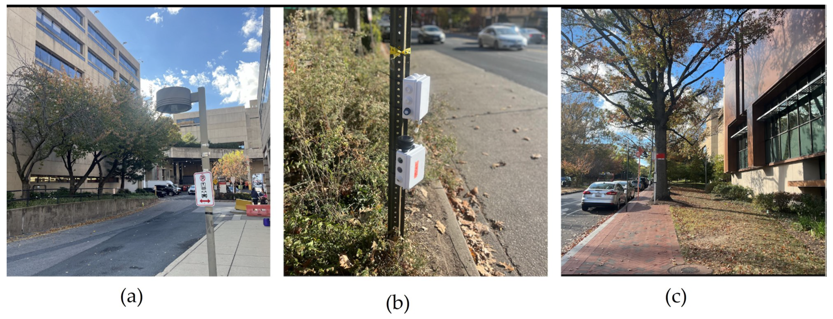
Figure 2.
(2a) Ozone (O3) and Temperature Node. (2b) Gases and PM Node.
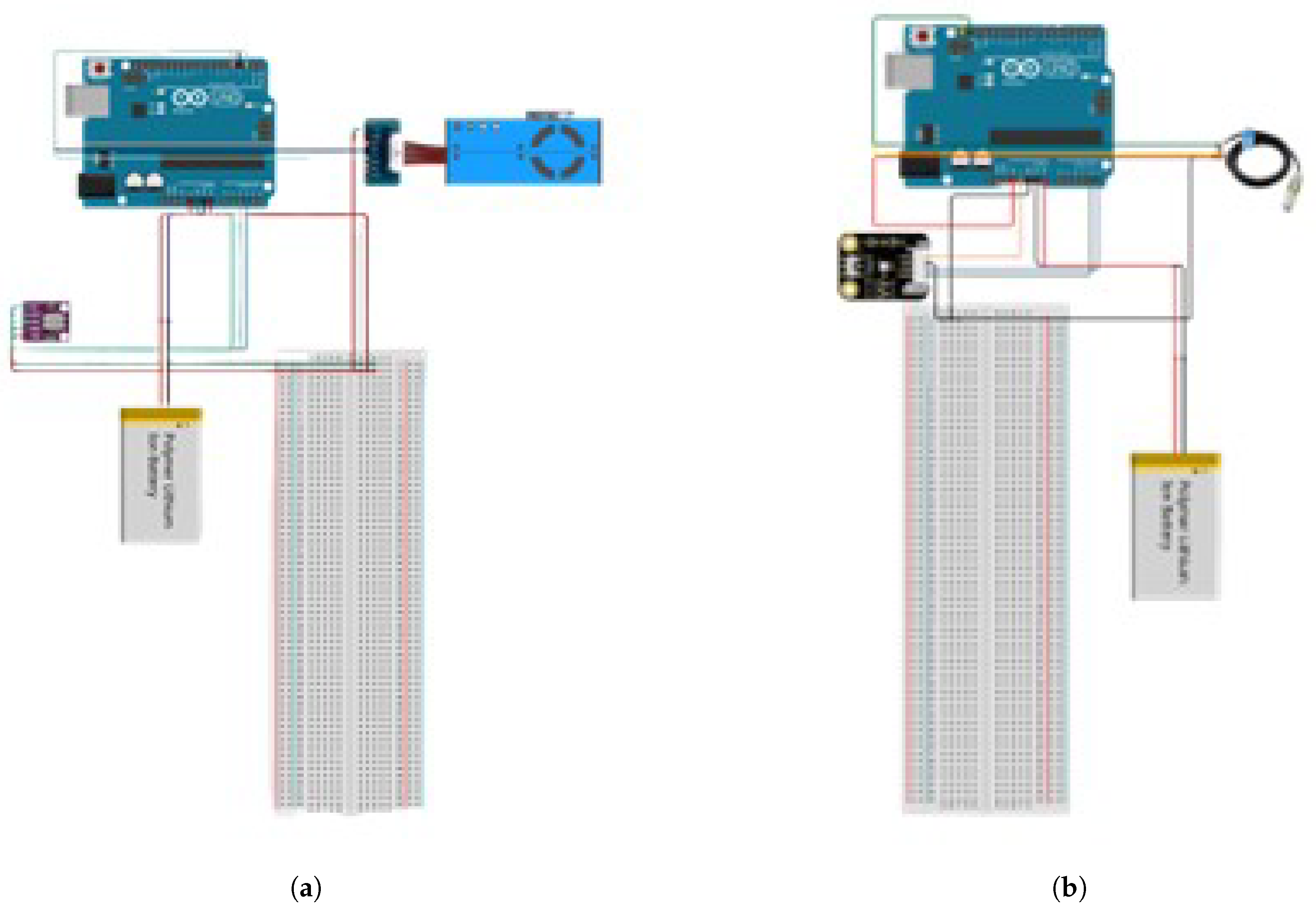
Figure 3.
Flowchart of Arduino UNO Data Collection Process.
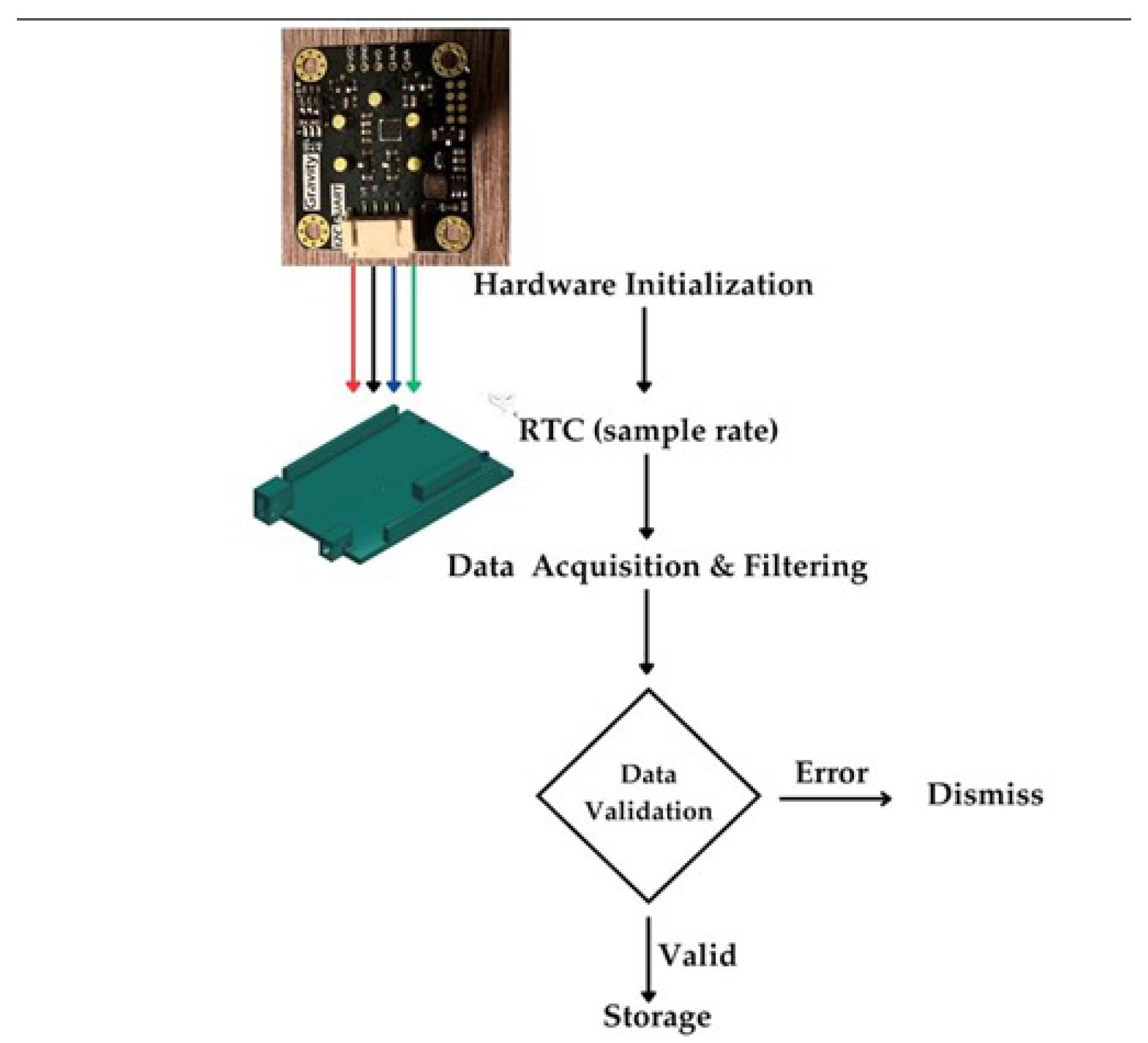
Figure 4.
Indoor Calibration Setup.
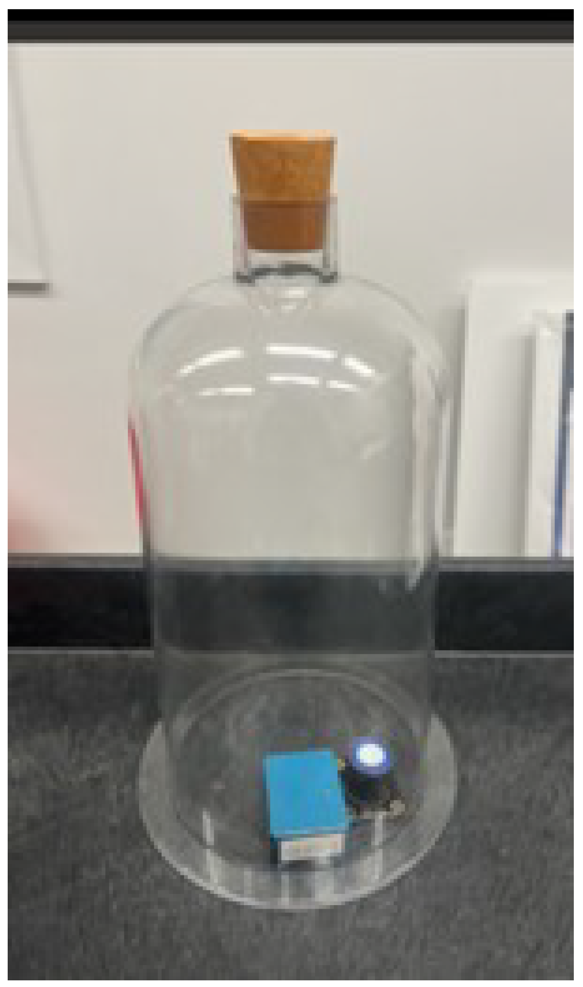
Figure 5.
(5a) Veazey St NW aerial-view (5b) Veazey St. NW 3-D simulation (ENVI-met).
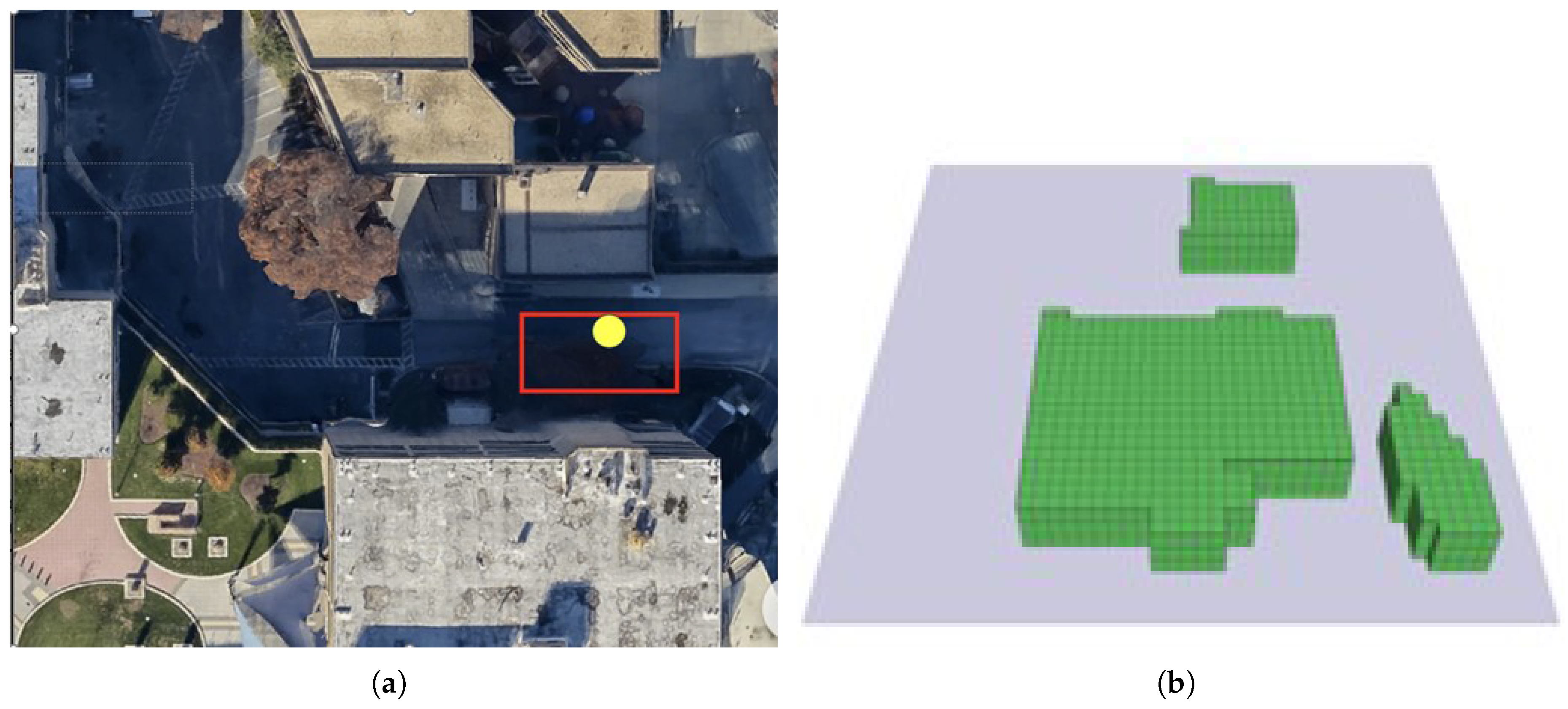
Figure 6.
(6a) Temperature Variation (6b) Wind Distribution.
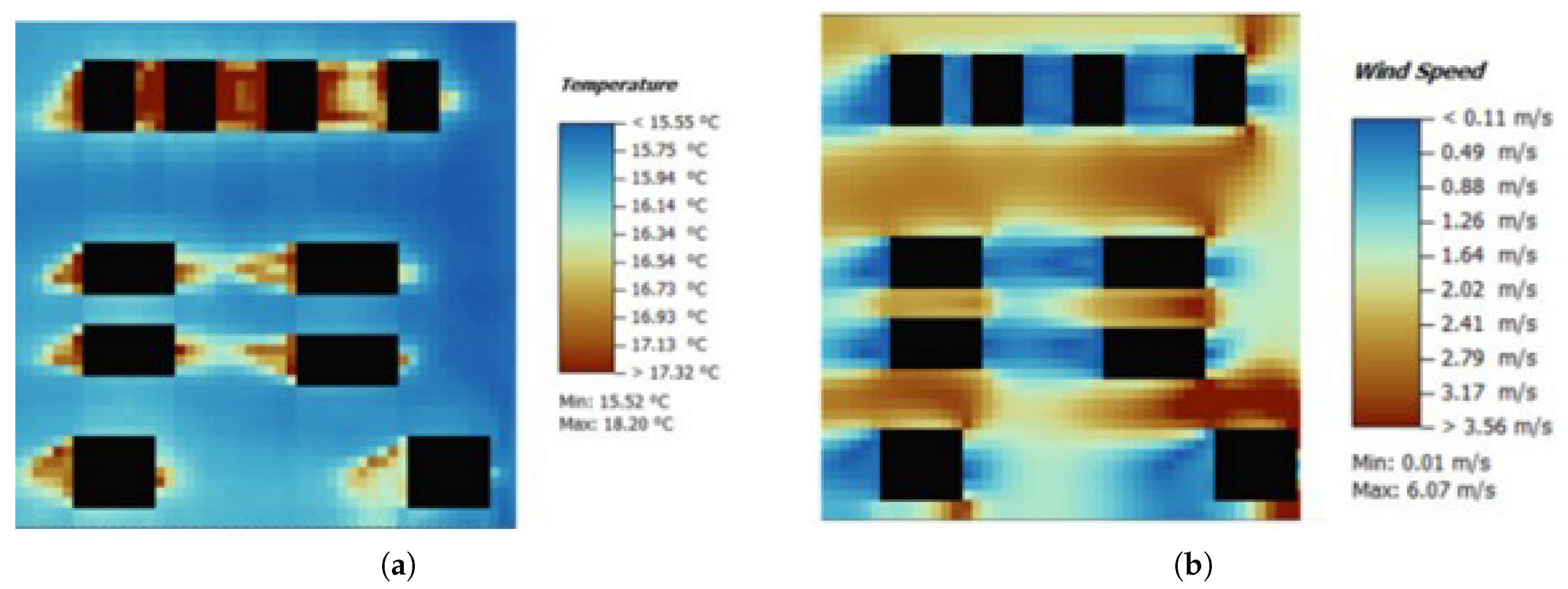
Figure 7.
SEN0385 Calibration: Raw vs. Calibrated Data and Adjusted Readings.
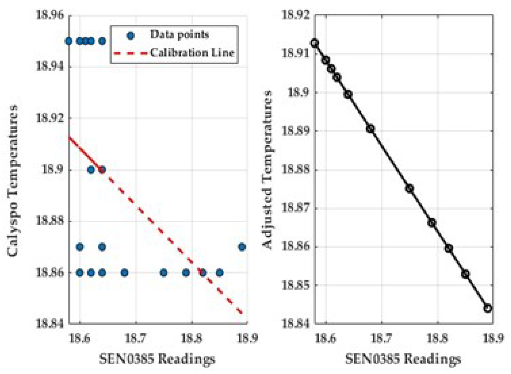
Figure 8.
SEN0472 (O3) Calibration: Raw vs. Calibrated Data and Adjusted Readings.
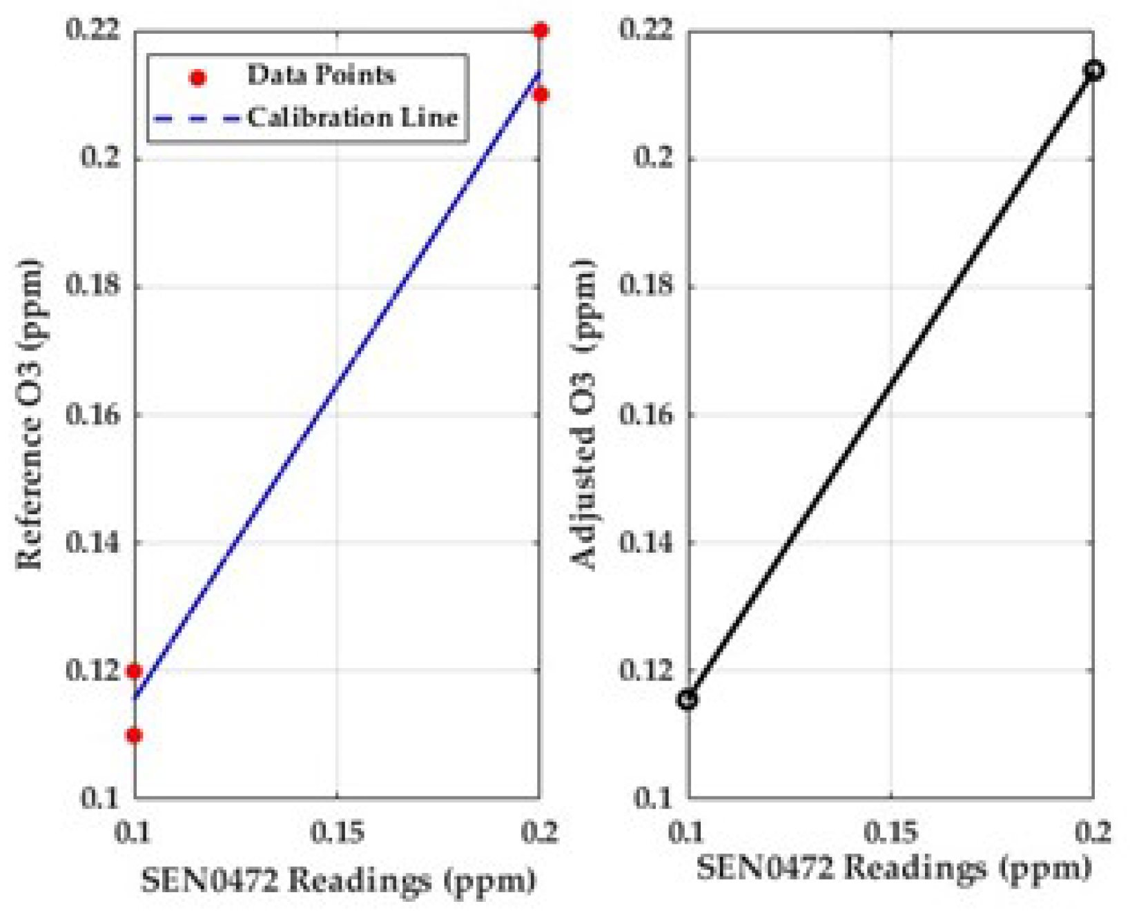
Figure 9.
MICS-6814 Calibration: Raw vs. Calibrated Data and Adjusted Readings.
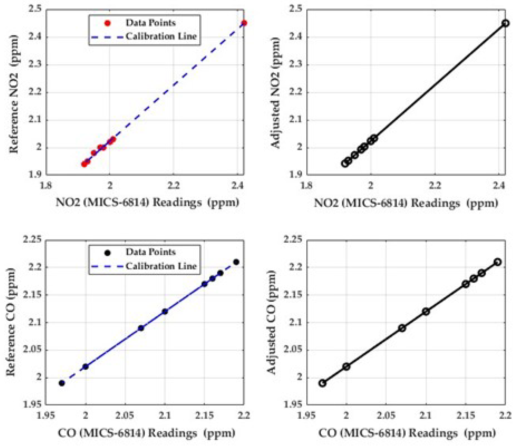
Figure 10.
Temperature Variation across Experimental Sites:(a) Temporal Trends (b)H/W Ration Comparison.
Figure 10.
Temperature Variation across Experimental Sites:(a) Temporal Trends (b)H/W Ration Comparison.
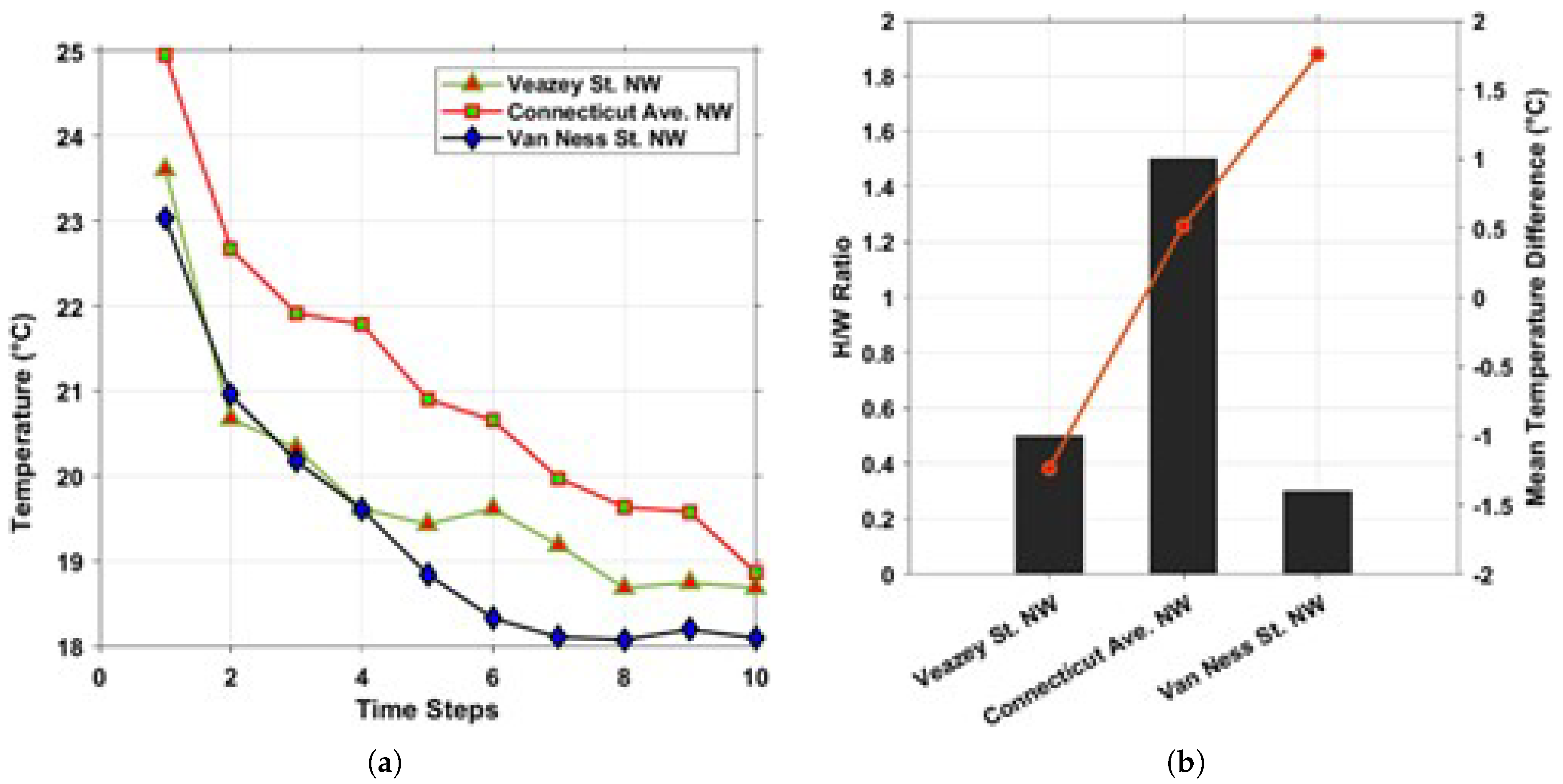
Figure 11.
(a)August 26, 2024 (b) October 4,2024 (c) November 6-7, 2024.
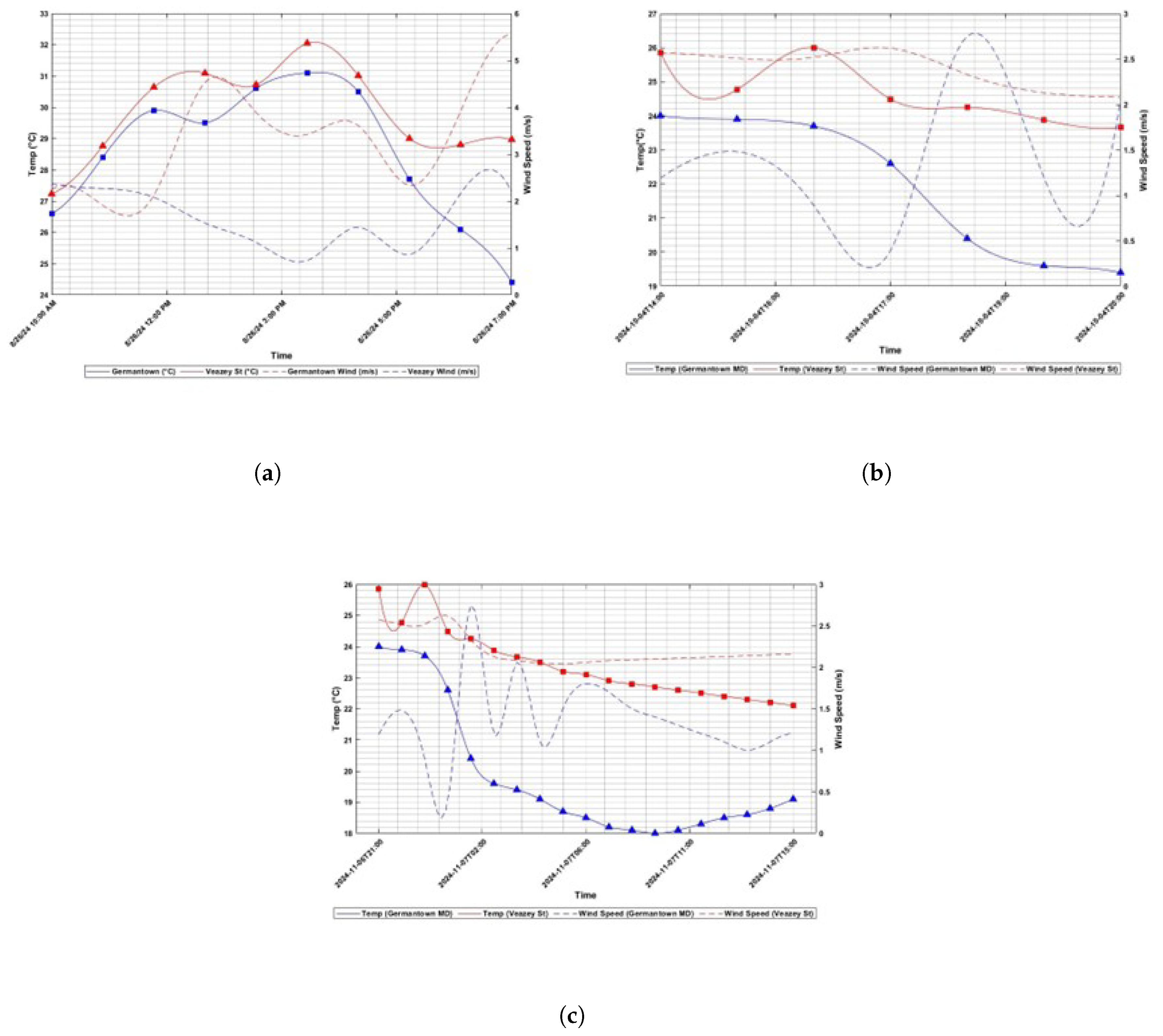
Figure 12.
Temperature Variation across Experimental Sites:(a) Temporal Trends (b)H/W Ration Comparison.
Figure 12.
Temperature Variation across Experimental Sites:(a) Temporal Trends (b)H/W Ration Comparison.
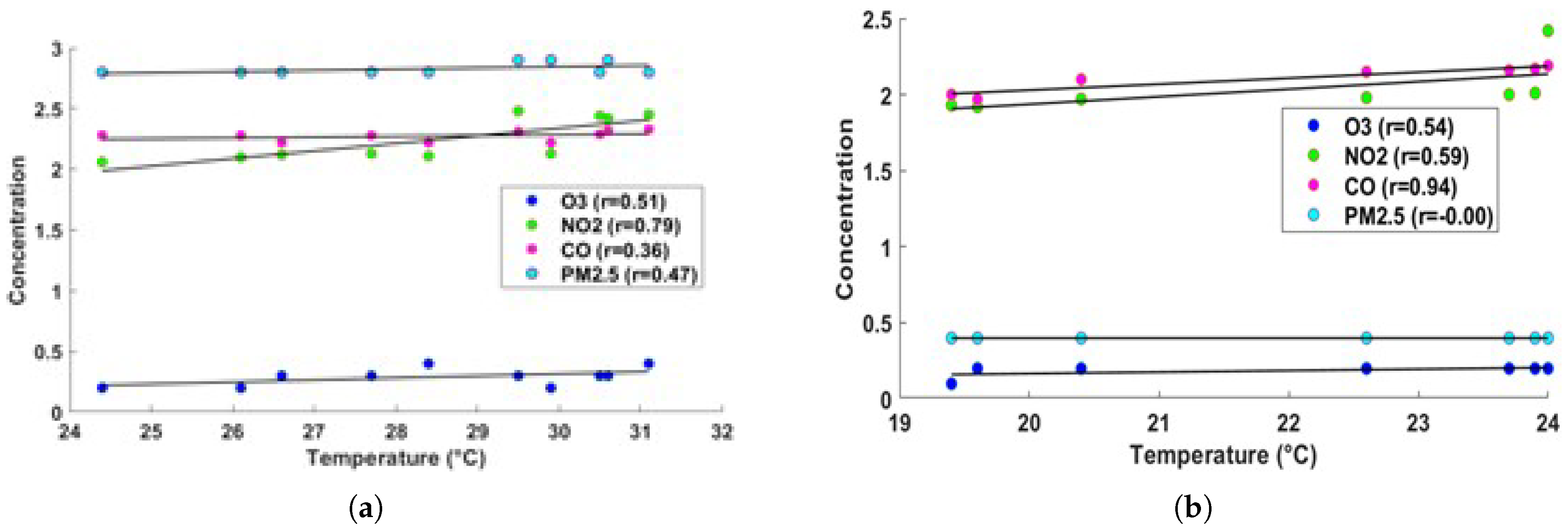
Figure 13.
CFD Simulations:Temperature (°C) :(a)August 26, 2024(b)November 6-7, 2024.
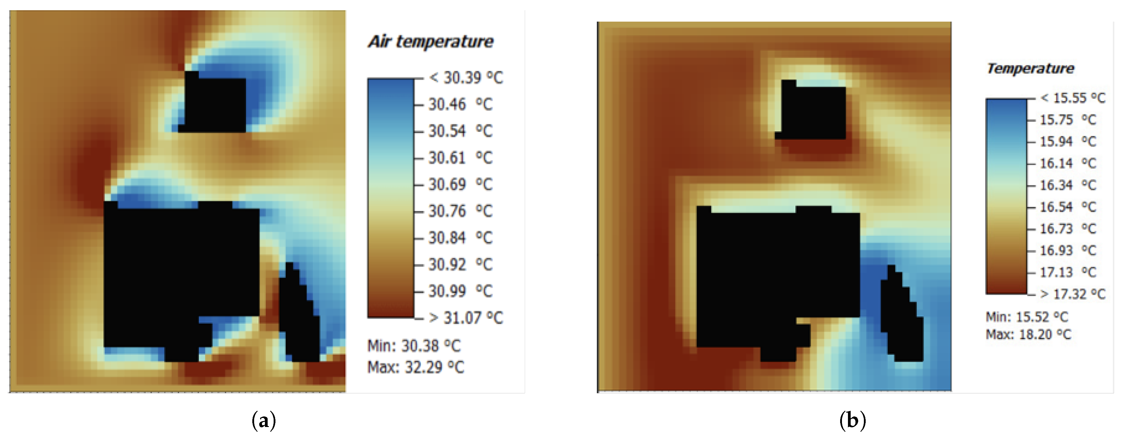
Figure 14.
CFD Simulations: Wind Speed(m/s) :(a)August 26, 2024(b)November 6-7, 2024.
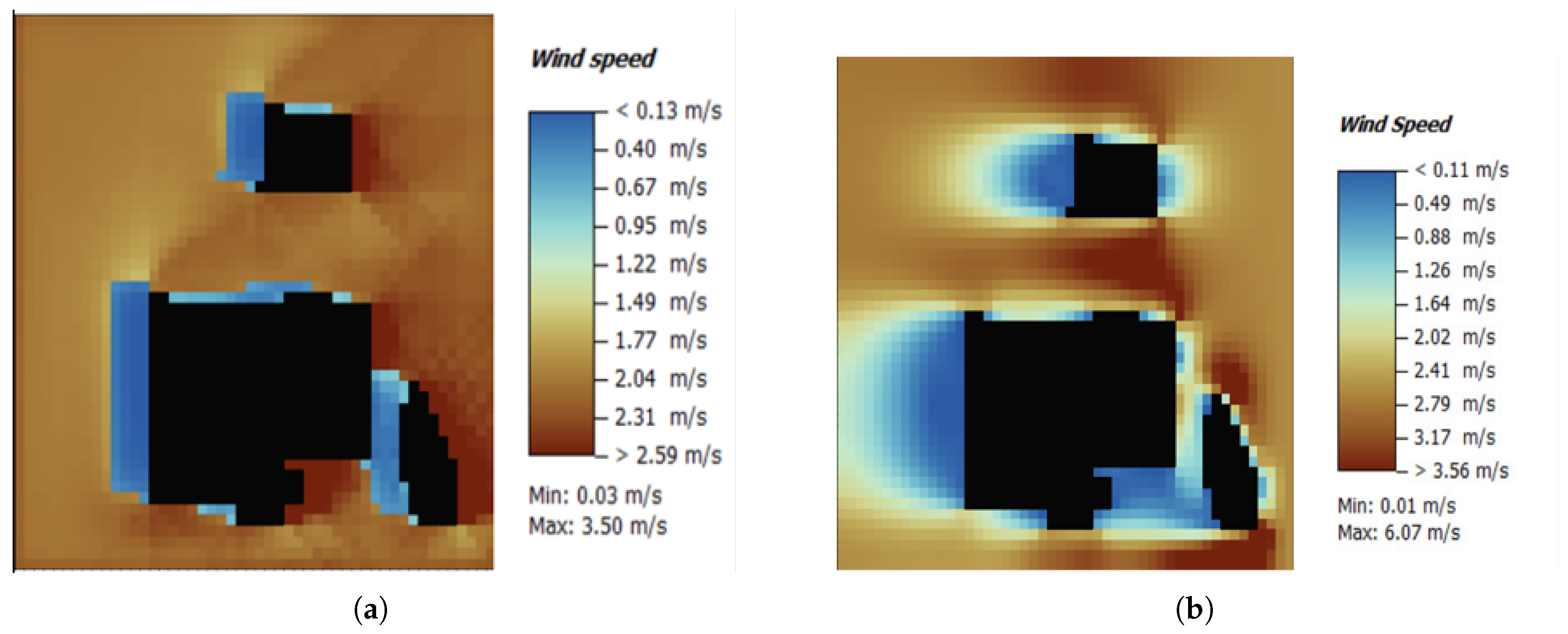
Figure 15.
CFD Simulations: PMV :(a)August 26, 2024(b)November 6-7, 2024.
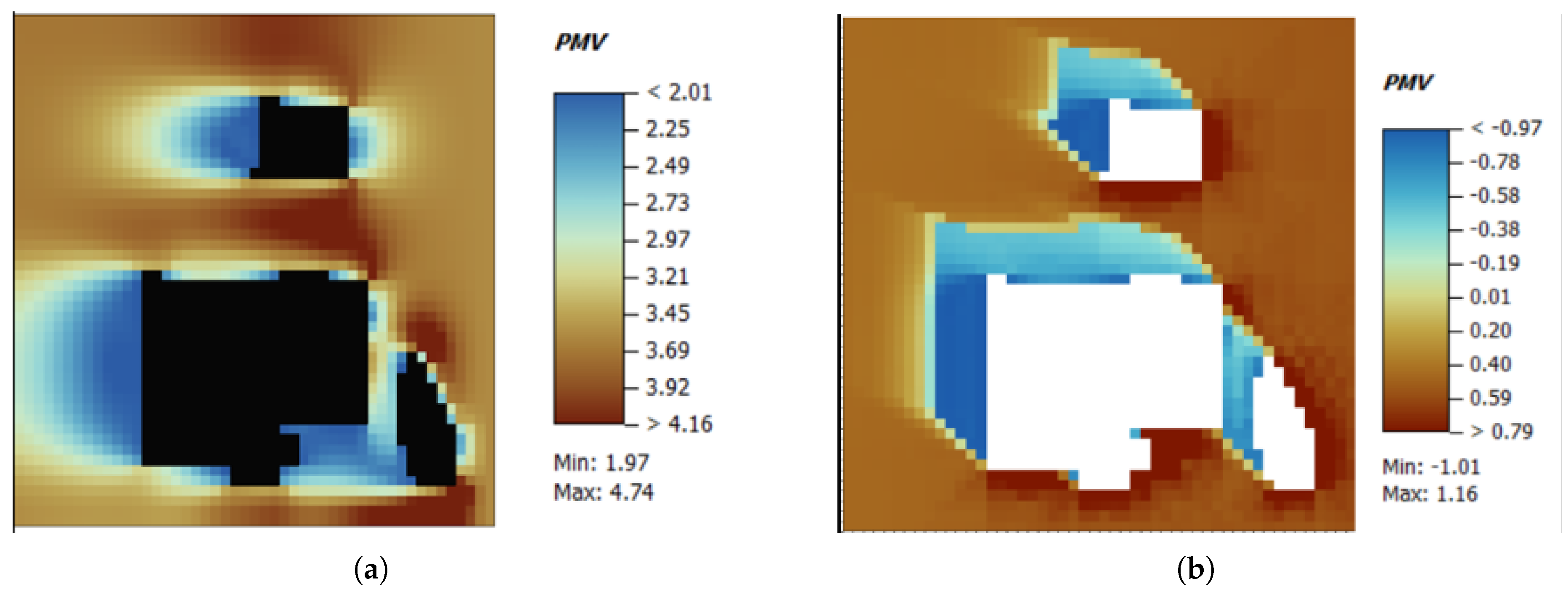
Figure 16.
CFD Simulations: PET :(a)August 26, 2024(b)November 6-7, 2024.
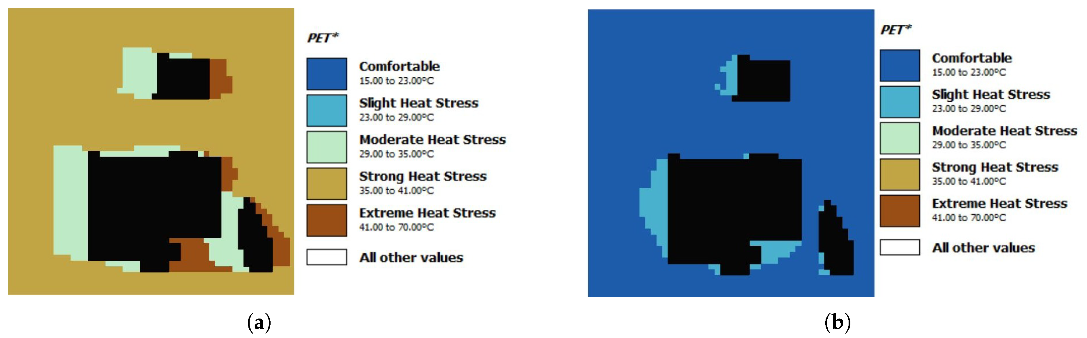

Table 1.
Sensor specifications.
| Sensor | Measured Parameters | Resolution | Accuracy |
|---|---|---|---|
| PMS5003 | PM1.0, PM2.5, PM10 | 0.1 µg/m³ | ±10% or ±1 µg/m³ |
| MICS 6814 (Gas Sensor) | CO, NO2, NH3 | 0.1 ppm | ±5% of reading or ±1 ppm |
| SEN0472 | O3 | 0.1 ppm | ±5% of reading or ±1 ppm |
| SEN0385 | Temperature, Humidity | 0.1°C (Temp), 1% (Humidity) | ±0.3°C (Temperature), ±3% (Humidity) |
| Ultrasonic Portable Solar Wind Instrument (Calypso) | Wind Speed, Wind Direction, Humidity | 0.1 m/s (Wind Speed) | ±2% (Wind Speed), ±3° (Wind Direction) |
1 Accuracy values are provided by sensor manufacturers.
Table 2.
Building Height, Street Width, and H/W Ratio for Different Locations.
| Location | Building Height (m) | Street Width (m) | Approximated H/W Ratio |
|---|---|---|---|
| Veazey St NW | 10-15 | 15-20 | 0.5-0.75 |
| Connecticut Ave NW | 20-30 | 10-15 | 1.5-2.0 |
| Van Ness St | 6-10 | 20-25 | 0.3-0.5 |
Table 3.
Data Validation Summary.
| Parameter | Experimental Range | Simulated Range | RMSE | R² |
|---|---|---|---|---|
| Air temperature(°C) August 26 | 30.38-32.29 | 30.12-32.10 | 0.75 | 0.91 |
| November 6-7 | 19.45 | 19.10-19.40 | 0.62 | 0.94 |
| Wind Speed(m/s) August 26 | 0.03-3.50 | 0.02-3.20 | 0.38 | 0.86 |
| November 6-7 | 0.04-4.50 | 0.03-4.10 | 0.42 | 0.88 |
Disclaimer/Publisher’s Note: The statements, opinions and data contained in all publications are solely those of the individual author(s) and contributor(s) and not of MDPI and/or the editor(s). MDPI and/or the editor(s) disclaim responsibility for any injury to people or property resulting from any ideas, methods, instructions or products referred to in the content. |
© 2025 by the authors. Licensee MDPI, Basel, Switzerland. This article is an open access article distributed under the terms and conditions of the Creative Commons Attribution (CC BY) license (http://creativecommons.org/licenses/by/4.0/).
Copyright: This open access article is published under a Creative Commons CC BY 4.0 license, which permit the free download, distribution, and reuse, provided that the author and preprint are cited in any reuse.


