The Monochromatic Resonator and the Interaction Between Light and Matter Under the Assumption That Photons Follow Classical Trajectories

Wolfgang Tiefenbrunner

doi:10.20944/preprints202502.1648.v1

Submitted:

20 February 2025

Posted:

20 February 2025

You are already at the latest version

Abstract

According to R. Feynman 1963-1965 [10], the interference pattern that appears on the observation screen in the double-slit experiment with light cannot be explained by classical physics. The detection probability is supposed to result from the superposition of all paths that the photon can take from the source to the detector, the light quantum is self-interfering. However, Jin et al. 2010 [11] showed that this is not necessarily the case. In their computer simulation, they assumed that the trajectory of a photon corresponds to that of a classical particle. Thus, the interference only occurs at the detector with the participation of several photons. Not every photon causes a detection.Tiefenbrunner 2024 [17] investigated the detector further and recognized that particle interference under this and some other conditions presupposes a monochromatic resonator (all permissible energy levels are integer (ℕ₀) multiples of a basal energy unit ε, where ε is also referred to as the ‘colour’ of the resonator). A monochromatic two-state system, e.g. a molecule that can only exist in two energetic states (ground and excited) and can only absorb one quantum (with respect to one ‘colour’), is, however, not sufficient for this. This prompted an evaluation of the significance of the monochromatic resonator for the Boltzmann-factor and Planck's radiation law. It turns out that the Boltzmann-factor and thus also the radiation law require resonators and hence are incompatible with two-state systems. The radiation law is derived using a kinetic model for the interaction of light with matter and without a priori use of the Boltzmann-factor, whereby it is also assumed that photons follow classical trajectories.

Keywords:

monochromatic resonator

;

double-slit experiment

;

Boltzmann-factor

;

Einstein's radiation laws

;

photon

;

light interference

;

Copenhagen interpretation

Subject:

Physical Sciences - Theoretical Physics

Introduction

In 1802, the English ophthalmologist T. Young conducted an experiment to clarify a dispute between I. Newton and C. Huygens on the nature of light—whether it consists of corpuscles or is a wave [19]. In the double-slit experiment, light can only travel from the source to the observation screen along two paths whose distances are often slightly different. An interference pattern appears in connection with the path difference, which indicates the wave nature of the light. On closer inspection, however, this pattern consists of many individual “dots”, as became apparent when G. I. Taylor repeated the experiment with a very weak light source and a very long exposure time in 1915 [15]. Prior to this, the wave interpretation had already been called into question with the explanation of the photoelectric effect by A. Einstein in 1905 [3]. This led to the concepts of wave-particle duality and “light quanta”. In particular, R. Feynman was convinced that every photon interferes with itself [9,10]. In the path integral formulation of quantum mechanics originally developed by G. Wentzel in 1924 [18], the detection probability of a particle is calculated as the superposition of all paths that the particle can take from the source to the detector. However, this is difficult to reconcile with the insight of A. Einstein in 1917 [6] that photons are obviously not emitted as a wave, because the emitting molecule experiences a momentum in a certain direction:

“If a body radiates the energy ε, it receives the rebound (momentum) ε/c if the entire amount of radiation ε is radiated in the same direction. However, if the radiation is emitted by a spatially symmetrical process, e.g., spherical waves, there is no rebound at all...there is no radiation as spherical waves” („Wenn ein Körper die Energie ε ausstrahlt so erhält der den Rückstoß (Impuls) ε/c, wenn die ganze Strahlungsmenge ε nach der gleichen Richtung ausgestrahlt wird. Erfolgt aber die Ausstrahlung durch einen räumlich symmetrischen Vorgang, z. B. Kugelwellen, so kommt überhaupt kein Rückstoß zustande...Ausstrahlung in Kugelwellen gibt es nicht“).

A. Einstein also rejected the Copenhagen interpretation of quantum theory, which states, among other things, that the properties of particles (such as position and momentum) are only determined by the act of measurement, which is incompatible with the cause-and-effect principle [8]. In his opinion, quantum theory as an ensemble theory is not capable of describing individual events or interactions at quantum level, but this does not necessarily mean that it is impossible.

According to R. Feynman, the double-slit experiment lies at the heart of quantum mechanics and is impossible to explain with classical physics [10]. In 2010, however, Jin et al. showed in a computer simulation that the results of the double-slit experiment can also be obtained if one assumes that the trajectory of a photon essentially corresponds to that of a classical particle; i.e., that it follows one and only one well-defined path and cannot interfere with itself [11]. However, the interference must then take place between different photons at the detector, which is of particular importance in this model. It must be assumed that, in addition to their frequency ν, they also carry information about their travel time (from source to detector) Δt modulo the oscillation period 1/ν (this can be imagined as the position of the hand on a clock face; the information is the phase at the time of absorption). The detector decides whether a detection (a “click”) occurs based on the information of several photons using a threshold function. This means that not every photon is detected. Jin et al. 2010 mention that their detector does not claim to be realistic.

The fundamental difference between R. Feynman’s views on the double-slit experiment and the view of Jin et al. 2010 can be shown as follows: We assume a coherent light source, so we can suppose that the photons match in phase when emitted. In the g-slit experiment, the detection probability is calculated as the square of the probability amplitude A, where g different paths from the source to the detector are possible, the photons each arrive at the detector with the phase information φ_i (i=1,...,g) and their relative frequencies are m_i (Σm_i=1; in the double-slit experiment: g=2). Quite idealized, this results in

\begin{array}{l} | A |^{2} & = \sum_{i} m_{i} e^{φ_{i} \sqrt{- 1}} \sum_{i} m_{i} e^{- φ_{i} \sqrt{- 1}} \\ = (m_{1} e^{φ_{1} \sqrt{- 1}} + m_{2} e^{φ_{2} \sqrt{- 1}} + \dots) (m_{1} e^{- φ_{1} \sqrt{- 1}} + m_{2} e^{- φ_{2} \sqrt{- 1}} + \dots) \end{array}

I.1)

This can be transformed into (Tiefenbrunner 2023, 2024) [16,17]:

| A |^{2} = \sum_{i, j} m_{i} m_{j} c o s α_{i j}

I.2)

where α_ij=φ_i–φ_j (i,j=1,...,g). In words: the detection probability results from the sum (over all photon-pairs) of the pairwise comparison of the photon phase at the time of arrival at the detector, divided by the square of the number of photons. Tiefenbrunner 2023 has pointed out that, due to a mathematical correspondence between the calculation of the cosine of the angle made by two intersecting vectors in the Cartesian coordinate system and the correlation coefficient, |A|² can also be interpreted as a mean correlation and thus as a measure of information [16]. In analogy to the Boltzmann entropy (also an information measure), which determines the proportion of energy that can be used as labour, the “quantum entropy”|A|² would determine the detectable proportion of energy that arrives at the sensor. This is because in this experiment not all photons are registered and this approach does not require “weird” physics. Usually, however, the double-slit experiment is interpreted with R. Feynman in such a way that all incoming photons are actually detected, |A|² therefore refers to the total energy that reaches the detector, and then all known effects that are contrary to common sense and associated with quantum theory are required. Is |A|² just a kind of entropy or something more? To answer this question, Tiefenbrunner 2024 started from the experiment by Jin et al. 2010, but chose a detector based on the pairwise comparison of photons (as suggested by the preceding arguments and Eq. I.2) and also on Einstein’s ideas on the interaction of light with matter (as interpreted by Feynman) [5,10]. Accordingly, the detector consists of idealised, ‘monochromatic’ two-state molecules, i.e., molecules that can exist in an energetic ground state or, alternatively, in an excited state with respect to a basal energy unit ε. In the excited state, it has absorbed a photon, taken on its energy ε and stores its phase information, which is now compared with the information of a second photon when it collides with it. Depending on the phase match, detection occurs with probability p_ij, while it fails to occur with the complementary probability 1–p_ij. If one chooses to fulfil some obvious conditions, we get:

p_{i j} = \frac{1 + c o s α_{i j}}{2} = {c o s}^{2} (\frac{α_{i j}}{2})

I.3)

For the probability of detection results [17]:

| A |^{2} = \sum_{i, j} m_{i} m_{j} p_{i j} - \sum_{i, j} m_{i} m_{j} (1 - p_{i j})

I.4)

This means that in order for the interference pattern to occur, there must be the option that a detection event is ‘cancelled’ by a non-detection. If the detector consists of independent, monochromatic two-state systems (molecules), the author believes that such behaviour is difficult, if not impossible, to imagine. It is conceivable that a non-detection on one molecule prevents the next detection, but of course this does not work in reverse order. Tiefenbrunner 2024 describes an entity that is capable of the desired behaviour [17]; it is a good old acquaintance from the early days of quantum theory, namely the ‘monochromatic resonator’ (an entitiy with the property that all permissible energy levels are integer (ℕ₀) multiples of a basal energy unit ε, where ε is also referred to as the ‘colour’ of the resonator). It can be said that the mathematics of ‘particle interference’ describes the kinetics of such a resonator. Whether it corresponds to a monochromatic molecule—which would then not be a two-state system—or whether several of them somehow form it in their entirety (as assumed in the cited paper) cannot be distinguished within the framework of the model. Here we want to investigate the hypothesis that the molecule itself is the resonator. It should have some properties that go beyond those of the original model (Figure 1).

In the model (Figure 1), the event that occurs with probability p_ij is the induced emission, while the absorption of a photon occurs with the complementary probability 1–p_ij. This is impossible for a two-state system, since absorption is only possible in the ground state Z₀ and emission only in the excited Z₁ and—since they cannot start from the same initial state—they are therefore independent events whose probabilities usually do not add up to one; in the monochromatic resonator, however, this is a realistic option (since Tiefenbrunner 2024 had assumed the two-state system, he did not recognise that absorption and induced emission are the alternative events, but postulated two different types of induced emission; a superfluous assumption) [17]. The observation of destructive interference is particularly interesting. In this case, induced emission and absorption balance each other out and nothing happens in the resonator at all. In the two-state system, however, induced emission will occur in half of all cases in which a photon hits a Z₁ molecule and absorption will always occur when a Z₀ particle is hit. This is a completely different result. In the case of non-coherent light, the kinetic constants for absorption α and induced emission β are also the same (Figure 1); the event is then determined by spontaneous emission on the one hand and the photon absorption by resonators that are in the ground state Z₀ on the other, where no phase comparison can take place. If light is coherent to a certain degree, however, it can be assumed that for Z_>0 induced emission is more likely than absorption.

The phase comparison of two photons requires an excited monochromatic molecule that has (somehow) stored the phase information of the absorbed photon. This argues against the single molecule corresponding to a resonator, as this would then have to have a very large, perhaps infinite, storage capacity (A. Einstein already recognised in 1925 that molecules cannot be regarded as independent of each other in quantum theory [7]). However, as we do not know what the link between the molecules looks like so that together they form the resonator, we will stick with the simpler idea of the ‘single-molecule-as-a-resonator’ for the moment.

The fact that the monochromatic resonator appears in a possible explanation of the interference pattern in the double-slit experiment is the reason for the following re-evaluation of its significance in the interaction between light and matter. Here we assume that photons can only follow one path and do not interfere with themselves. As they are not carriers of a charge, they cannot generally interact directly with each other, but they can of course interact with matter and thus indirectly. We develop a kinetic model because we assume with A. Einstein that the mode of single-event interactions can in principle be understood beyond the measurable. In contrast to his kinetic model of 1916 [5] and other derivations of the radiation law, we will not use the Boltzmann-factor a priori. We will show that this would be unwise. We will start with the Boltzmann model of 1877, in which the molecule already has the properties of a monochromatic resonator [1].

1). The Boltzmann Model: Random Processes and Probability

In 1877, L. Boltzmann [1] presented a simple but extremely interesting model (in contrast to many of his contemporaries in the field of physics, who were influenced by E. Mach, he was convinced of the existence of molecules):

“Let’s assume we have n molecules. Each of them is capable of generating the living force 0, ε, 2ε , 3ε . . . pε, and let these living forces be distributed in all possible ways among the n molecules, but in such a way that the total sum of the living force of all molecules … is always the same.” (living force=kinetic energy. „Wir nehmen an, wir hätten n Moleküle. Jedes derselben sei imstande, die lebendige Kraft 0, ε, 2ε , 3ε . . . pε anzunehmen, und zwar sollen diese lebendigen Kräfte auf alle mögliche Weise unter den n Molekülen verteilt werden, jedoch so, daß die Gesamtsumme der lebendigen Kraft aller Moleküle immer dieselbe ... ist.“)

In other words, in addition to the existence of molecules, he also postulated in his model (which corresponds to the monochromatic resonator), but not in reality, the existence of discrete energy quanta ε. The relative simplicity of the mathematical treatment of the problem was his motivation for this step.

“If we know how many of these n molecules have the living force zero, how many have the living force ε, etc., then we say: The distribution of the living force among the molecules, or the state distribution, is given to us.” („Wenn wir wissen, wie viele von diesen n Molekülen die lebendige Kraft Null, wie viele die lebendige Kraft ε usw. besitzen, so sagen wir: Die Verteilung der lebendigen Kraft unter den Molekülen, oder die Zustandsverteilung ist uns gegeben.“)

It can be assumed that the interaction of molecules and the exchange of quanta leads to an equilibrium at a certain state distribution (energy distribution). However, Boltzmann did not investigate the kinetics of this process (as we will do), but chose a different approach in the aforementioned publication [1]. He searched for and found the dispersion equilibrium by determining what he considered to be the most probable state distribution. It should be possible to assign different ‘molecular arrangements’ (possible permutations) to each state distribution and he assumed that they could all occur with equal probability. The state distribution with the largest number of possible molecular arrangements (he called them ‘Kompexionen’) would therefore be the one that could be observed with the greatest probability. How he went about this is by no means self-explanatory and therefore needs to be explained.

In principle, he used the rules of the ‘shell game’, in which the aim is to find the shell under which the pea (or another small object) is located. In this game, the shells have individuality, whereas the peas do not. Boltzmann gives an example in which he distributes seven peas (quanta) among as many shells (molecules). One possible distribution of states is given, for example, by the fact that all the quanta are in one molecule and the other six are therefore empty. According to his rules, the arrangements 0000007 and 0070000 are different; there are therefore a total of seven permutations for this energy distribution. If, on the other hand, each molecule has one quantum: 1111111, there is only one possible arrangement because no distinction is made between the quanta; they have no individuality (e.g., this would be 1 and 1′). Since all possible arrangements of seven quanta in seven molecules should be equally probable, the energy distribution discussed first has a higher probability. Accordingly, the state distribution consisting of three empty molecules, two singly occupied and one doubly and one triply occupied (e.g., 0001123) is the most probable, because in this case there are 420 possible permutations and in no other case more (with seven molecules and as many quanta there are 15 different energy distributions, but none allows more arrangements than the one mentioned; the next highest number would be 140, which is significantly less).

Here we use a different notation than Boltzmann: let N be the number of all molecules, Q the number of quanta (‘Q’ is the number of quanta with energy content ε, so we think Q_ε, but write only Q for convenience), and N_i the number of molecules harbouring i quanta (with i=0,...,Q). Then the number B of permutations per state distribution is given by:

B=N!/Π_i(N_i!),

thus B(0001123)=7!/(3! 2! 1! 1!) = (7 6 5 4)/2 = 420.

As already mentioned, Boltzmann assumes that the state distribution in which the system will be found when a large number of molecules and quanta are present is the most probable, i.e., the one with the most possible arrangements. He therefore searches for the state distribution for which B is maximal (or Π_i(N_i!) is minimal, since N! is the same for all energy distributions). Using the gamma function and Stirling’s formula for approximating large factorials, he shows that this corresponds to an exponential distribution for which the following applies:

N₀=N²/(N+Q)

and

N_i+1=N_i Q/(N+Q)

If we further define that n_i=N_i/N and q=Q/N (again, we think q_ε, but are convenient and only write q), this results in:

1.1): n₀=1/(1+q)

and

1.2): n_i+1=n_i q/(1+q)

From this follows:

1.3): n_i=[1/(1+q)][q/(1+q)]ⁱ

However, one could criticise Boltzmann’s approach by mentioning that the probability (what is probable and what is not) depends on the underlying random process. Boltzmann also constructed this as well:

‘Let’s assume we have an urn containing an infinite number of pieces of paper. On each of them is one of the figures 0, 1, 2, 3, 4, 5, 6, 7; each figure is on the same many pieces of paper and the probability of being drawn is the same for each one. We now draw seven pieces of paper ...’ („Wir nehmen an, wir hätten eine Urne, in der sich unendlich viele Zettel befinden. Auf jedem der Zettel steht eine der Zahlen 0, 1, 2, 3, 4, 5, 6, 7; und zwar steht jede Zahl auf gleich vielen Zetteln und ist die Wahrscheinlichkeit gezogen zu werden für jeden Zettel dieselbe. Wir ziehen nun sieben Zettel ...“).

This is of course repeated very often and gives him a random process that actually generates with the greatest probability the energy distribution that has the most permutations. However, Boltzmann now has to supplement this process with a selection procedure because the sum of the digits over the seven slips of paper must always equal seven due to the conservation of energy. He has to eliminate all ‘Septernen’ for which this is not the case. This of course means that his procedure is no longer purely random.

There are certainly other conceivable random processes with other most probable outcomes. Let’s assume that we initially have nothing but ‘empty’ (ground state) molecules and a bag full of quanta. If we now select one of the molecules at random and fill it with a quantum from the bag and repeat this until the bag is empty, we obtain an energy or state distribution that corresponds to the Poisson distribution. The most probable one is then given by

n_i=(qⁱ/i!) e^-q

resp.

n₀=e^-q

and

n_i+1=n_i q/i,

which obviously does not correspond to the Boltzmann distribution. Figure 2 shows this Poisson energy distribution for q=1 (left) and q=5 (right) for one million molecules (white curve). Also shown is the result of a Monte Carlo simulation (red) for the process described (the agreement is so big that one of the two curves had to be drawn slightly offset so that it could be seen at all). The third, yellow curve shows the Boltzmann distribution, which obviously does not follow from the random process described above.

Which state distribution is the most probable has no influence on the Boltzmann entropy, for which only N and Q are relevant:

1.4): S = k ln Ω

with

1.5): $Ω = (\begin{matrix} N + Q - 1 \\ N - 1 \end{matrix})$

which results in Ω = 1716 for seven quanta and seven molecules (Ω =13!/(6!(13-6)!); k is the Boltzmann constant). Ω is the total number of possible arrangements of quanta on the molecules (or the number of ‘Komplexionen’).

If there are several plausible random events in which completely different results are the most probable, Boltzmann’s argumentation can hardly be considered satisfactory. We therefore try to obtain his result in another way, within the framework of a kinetic model.

2). A Simple Kinetic Model of Energy Exchange Between Molecules

Like Boltzmann, we assume that the individual molecule or particle is a monochromatic resonator. Every interaction between two molecules, which we want to assume takes place randomly, should result in the transfer of exactly one quantum. The transfer cannot start from a molecule that is empty, i.e., that does not carry a quantum, but otherwise there are no further rules that determine which molecule is the donor and which is the recipient.

In principle, we distinguish between two possible processes:

1) Absorption of a quantum: The transition from an (i-1)-particle to an (i)-molecule occurs with probability: n_i-1(1–n₀), since Σn_i=1. Every molecule, with the exception of a (0)-particle, can transfer a quantum and the probability of two molecules meeting depends on their relative frequency.

2) Release of a quantum: The transition from an (i)-molecule to an (i-1)-molecule occurs with probability n_i, since each particle can absorb a quantum.

A: We now ask about the probability that an (i)-particle will be created. This is the case if:

1) An (i-1)-particle absorbs a quantum. The probability of this is n_i-1(1-n₀).

2) An (i+1)-particle releases a quantum. The probability of this is n_i+1.

B: When is a (i)-particle lost? Whenever:

1) An (i)-particle absorbs a quantum. The probability of this is n_i(1-n₀).

2) An (i)-particle loses a quantum. The probability of this is n_i.

This results in the kinetic equation (i=0, … ,Q):

2.1): Δn_i/Δt = n_i+1 + n_i-1 (1–n₀)—n_i − n_i (1–n₀)

In particular:

2.2): Δn₀/Δt = n₁ − n₀ (1–n₀)

and:

Δn_Q/Δt = n_Q-1 (1–n₀) − n_Q

In equilibrium, the following must apply: Δn_i/Δt=0. According to Eq. 2.2, this initially results in:

n₁ − n₀ (1–n₀) = 0

2.3): n₁ = n₀ (1–n₀)

And from Eq. 2.1 follows:

n_i+1 + n_i-1 (1–n₀) − n_i − n_i (1–n₀) = 0

2.4): n_i+1 = n_i + (n_i − n_i-1) (1–n₀)

Of course, the fact that n_i+1 depends on n_i as well as n_i-1 and n₀ is a problem here. Let us assume that it can be shown that n_i+1=n_i(1–n₀), a conclusion that can be drawn by generalizing Eq. 2.3. Then, of course, the following would also apply: n_i=n_i-1(1-n₀) and therefore n_i-1=n_i /(1-n₀). If we replace n_i-1 in Eq. 2.4, we obtain

n_i+1 = n_i + (n_i–n_i/(1–n₀)) (1–n₀)

A brief calculation returns the result:

2.5): n_i+1 = n_i (1–n₀)

which shows that the assumption was correct. If, on the other hand, we had assumed that n_i+1=n_i(1–n_i) or n_i+1=n₀(1–n_i) according to eq. 2.3, for example, it would have been shown very quickly that these assumptions were incorrect.

Eq. 2.5 is much simpler than Eq. 2.4, but we do not know n₀ and therefore also not the state distribution. It is now time to remind ourselves of the boundary conditions:

n₀ + n₁ + n₂ + … + n_Q = 1 molecules

2.6): n₁ + 2n₂ + 3n₃ + … + Qn_Q = q quanta

If there is an exponential distribution, which is described by Eq. 2.5, the first terms are particularly important and the factor Qn_Q can be ignored as an upper limit for reasonably large Q. From Eq. 2.6 in conjunction with Eq. 2.5 then follows:

q = n₀ (1–n₀) + 2 n₀ (1–n₀)² + 3 n₀ (1–n₀)³ + …

2.7): q = n₀ [(1–n₀) + 2 (1–n₀)² + 3 (1–n₀)³ + … ]

We take from a collection of formulas:

1/(1–ξ)² = 1 + 2 ξ + 3 ξ ² + …

from which it follows by multiplication with ξ that

ξ/(1–ξ)² = ξ + 2 ξ ² + 3 ξ ³ + …

Eq 2.7 therefore takes the form:

q/n₀ = (1–n₀)/[1 − (1–n₀)]² = (1–n₀)/n₀²

q = (1–n₀)/n₀

This can now be used to calculate n₀:

2.8): n₀ = 1/(1+q)

And from Eq. 2.5 and Eq. 2.8 finally follows:

2.9): n_i+1 = n_i q/(1+q)

Eq. 2.8 corresponds to Eq. 1.1 and Eq. 2.9 is identical to Eq. 1.2. We have therefore derived the Boltzmann distribution from assumptions about the kinetics of quantum exchange between the molecules. If Boltzmann had also followed this path, he would have noticed something very strange. We had to assume that the probability of quantum transfer from one molecule to the next, and in particular the direction in which it takes place, is independent of the number of quanta contained in the molecules involved. Would it not be much more obvious to assume that the transition from a molecule containing, say, four quanta to one containing only two quanta is twice as frequent as the transition in the opposite direction? Or, more generally, shouldn’t the transition occur preferentially in the direction of the molecules with fewer quanta? If so, the Boltzmann distribution would not be the one observed. It would not be the most probable one. The puzzle was first solved by A. Einstein in 1916, when he recognized that the molecules or monochromatic resonators do not interact directly with each other [5]. Rather, the quantum transfer takes place between the resonator and a “quantum reservoir”, the electromagnetic field. And in this case, the frequency with which interaction occurs actually depends, as one might expect, on how many quanta the reservoir contains.

3). Boltzmann’s Approximation for the State Distribution

In the case that q is very large (q>>1), Boltzmann gives approximations for Eq. 2.8 and Eq. 2.9

3.1): n₀ = 1/(1+q) ≈ 1/q
3.2): P = n_i+1/n_i = q/(1+q) ≈ exp(-1/q)

(using the first two terms of the Taylor series for the exponential function: exp(ξ) ≈ 1+ξ, if ξ is close to zero and the transformation exp(1/q)=1+1/q) and therefore:

3.3): n_i=(1/q) exp(-i/q)

In the model, q is the average number of quanta per monochromatic resonator and ε is the energy per quantum. We can of course write

q = qε/ε

Then qε is the mean energy per resonator and can therefore be replaced by kT, the average energy per molecule, because only quanta of ‘colour’ ε contribute to the energy of the resonators (this is, however, a simplifying assumption that is completely unrealistic and is therefore already rejected in the next chapter), because for Boltzmann, resonator and molecule are the same (k: Boltzmann constant; T: temperature). This results in

3.4): q = kT/ε

In this way, q acquires a physical meaning (later, however, we replace Eq. 3.4 with qε ≤ kT). This finally results in

3.5): P = n_i+1/n_i ≈ exp(-ε/(kT))

This could be referred to as the “monochromatic Boltzmann-factor”, which flows into various derivations of the radiation law either directly or via entropy as a prerequisite and is therefore very important. The question now is whether its a priori use can be justified. We will examine this with an example, namely for quanta with the energy of visible light and for molecules that have the surface temperature of the sun (approx. 6000°C). We choose light with a wavelength of 500 nm, from which we can calculate the energy of the quantum using ν=c/λ and ε=hν (ν: frequency, λ: wavelength, c: speed of light, h: Planck’s quantum of action). This results in q=0.22 if we utilize Eq. 3.4. This is far too small a number to justify the use of Boltzmann’s approximation, e.g., for the derivation of the radiation law; it would give a completely wrong result. Even if one takes into account that different quanta contribute to the energy of a molecule, q does not become larger as a result; quite the opposite.

Feynman also uses the “monochromatic Boltzmann-factor” in his (pick and choose from everywhere) derivation of the radiation law [10]. He starts from a two-state system (n₀ is the relative number of molecules in the ground state Z₀ and n₁ is the number of molecules in the higher-energy, excited alternative state Z₁). In this system, however, n₀=1–n₁ and furthermore q=n₁ (which also means that q≤1 and hence cannot be a large number) and therefore:

3.6): n₁/n₀ = q/(1-q)

instead of Eq. 2.9 (n_i+1/n_i = q/(1+q)). In this case, however, the approximation that leads to the monochromatic Boltzmann-factor is invalid! We obtain

P=1/(ε/(kT)-1)

which provides positive values for P if ε>kT or q<1 (i.e., only some of the molecules carry a quantum).

Another approach that is difficult to accept and is occasionally carried out is the equalization of approximation and exact solution. From Eq. 3.2 (P=q/(1+q)) we obtain q=P/(1-P). By substituting the approximation for P, i.e., P≈exp(-ε/kT) and completely forgetting that it is an approximation and how we arrived at it, we obtain

3.7): q=1/(exp(ε/kT)-1)

If we calculate q for our example (temperature of the sun’s surface etc.), the result is: q=0.01 (in the holochromatic model, however, it turns out that Eq. 3.7 makes perfect sense).

It follows from all this that it is better to avoid the a priori use of the “monochromatic Boltzmann-factor” in our considerations on the interaction of light and matter.

4). The holochromatic molecule and the Boltzmann-factor

The Boltzmann-factor describes the relationship between particle energies and abundances as a function of temperature. For the holochromatic molecule, which can absorb quanta of different ‘colours’ (ε, aε, bε ...; with a, b,...ϵ ℝ₀⁺), it could be formulated as follows:

4.1): P_{ε(1,a,b,...)} = exp(-ε(1+a+b+...)/(kT))

We assume that this equation correctly describes reality and then draw certain conclusions from this assumption (just as A. Einstein did in 1916 with the radiation law). From the previous chapter, we know that for the two-state system holds with respect to quanta of energy (or ‘colour’) ε (Eq. 3.6)

P_ε = n₁/n₀= q_ε/(1-q_ε)

respectively for the monochromatic resonator (eq. 2.9):

P_ε = n_i+1/n_i = q_ε/(1+q_ε)

The next step would be a dichromatic molecule that can accommodate two quanta with the different energies (‘colours’) ε and η, where η=aε. We first choose a two-state molecule, i.e., one that can be in the Z₀ or Z₁ state (at two different energy levels) for both ‘colours’ ε and η. We also assume that the combination of quanta in the molecule population takes place without mutual influence of the ‘colours’. Then the molecular abundances n₀₀, n₀₁, n₁₀, n₁₁ result in the two-state system according to the following Table 1, which takes into account that the molecule can be in the ground or excited state with respect to each colour:

This gives the ratios of the frequencies for molecules at different energy levels:

n₁₁ /n₀₁ = q_εq_aε / ((1-q_ε)q_aε) = P_ε

n₁₁/n₁₀ = q_εq_aε / (q_ε(1-q_aε)) = P_aε

n₁₁/n₀₀ = q_εq_aε /((1-q_ε)(1-q_aε)) = P_ε P_aε

and of course:

n₀₁/n₁₀ = (1-q_ε)q_aε/(q_ε(1-q_aε)) = P_ε /P_aε

We change the notation a little by defining P_ε_{, aε}:

P_ε_{, aε} = P_ε_{(1, a)} = n₁₁/n₀₀ = P_ε P_aε

This can be extended for the holochromatic molecule:

4.2): P_{ε (1,a,b,...)} = P_ε P_aε P_bε …

It follows that:

ln(P_ε _(1,a,b,...)) = ln(P_ε P_aε P_bε …)

P_ε _(1,a,b,...) = exp(lnP_ε + lnP_aε + lnP_bε + ...)

for

lnP_ε= -ε/kT

etc. then follows:

P_ε_(1,a,b,...) = exp(-ε(1+a+b+...)/(kT))

i.e., the holochromatic Boltzmann-factor (Eq. 4.1). Provided that the assumption that the colours have no influence on each other is valid, it must therefore apply for the monochromatic one (see also Eq. 3.5):

4.3): P_ε = exp(-ε/kT)

For the dichromatic resonator, one can proceed in a completely analogous way to the two-state system by examining neighbouring states Z_i+1, Z_i or Z_j+1, Z_j (in the resonator, molecules can of course also differ in the energy budget due to the presence or absence of several quanta of the same colour, so the states do not necessarily have to be neighbouring) and the relation n_i+1,j+1/n_i,j. One then arrives via the intermediate stage

P_ε _,aε = P_ε_(1,a) = n_i+1,j+1/n_i,j = P_ε P_aε

at Eq. 4.3. However, as the previous chapter has shown, Eq. 4.3 is not a possible result for the two-state system but only for the resonator and even then only as an approximation for large q.

There is obviously a contradiction here, because in reality Eq. 4.3 also applies for small q. On the one hand, an attempt to explain this would be to assume that the totality of all quanta of different colours in the holochromatic molecule balances each other out (there are many quanta present across all colours) in a way that still allows the different colours to be described as independent of each other; on the other hand, many two-state systems could somehow form a resonator together (the assumption of Tiefenbrunner 2024 [17]). In any case, independent holochromatic two-state molecules are not an option.

5). The Planck-Einstein Model: Interaction of Radiation and Matter

We must now integrate the quantum reservoir, the electromagnetic field, into our model by considering how the field and the molecule (the resonator) interact with each other. A. Einstein already did this in 1916 [5]. His kinetic model was later interpreted, for example by Feynman, in such a way that, apart from the energetic ground state Z₀, there is only an excited Z₁ with respect to a certain colour (Figure 2A), which − as we have seen—is very problematic if the Boltzmann-factor is used [10]; A. Einstein writes, however: “Each molecule is only capable of a discrete series Z₁, Z₂ etc. of states with the energy values ε₁, ε₂ etc.” („Jedes Molekül sei nur einer diskreten Reihe Z₁, Z₂ usw. von Zuständen fähig mit den Energiewerten ε₁, ε₂ usw.“), but does not explain whether successive states in his model are equidistant with respect to the energy level (Figure 3B). In 1916, however, he denoted his model as a monochromatic resonator, the properties of which he had already defined more precisely in 1914 [4], including the fact that all allowed energy states are discrete (ℕ₀) multiples of an energy unit, a quantum. It is this monochromatic resonator that we will now examine in more detail. Molecule and resonator are identical.

According to A. Einstein, we distinguish between three types of interaction between a field—or a quantum of the field, i.e., a photon—and a molecule, whereby we assign a kinetic constant (α, β, γ in Figure 1 and Figure 3) to each of them. These are absorption (α), induced (β) and spontaneous (γ) emission. Our model (Figure 3B) allows any number of excited states for the resonator in addition to the ground state Z₀, whereby there is a distance ε=hν between Z_i and Z_i+1, i.e., it is equidistant (‘ladder-like’) for all i, whereby the i of the current state is the sum of quanta per resonator. Nevertheless, just as in a two-state system, there is no emission cascade; only one photon is released per emission event, no matter whether it’s induced or spontaneous (this assumption is crucial for the resulting of Planck’s law of radiation). We also presume that the light is not coherent (or only has negligible coherence). Then the monochromatic resonator of Figure 1 is simplified to Figure 3B, because we do not have to consider the phase information of the photon.

A. Einstein compared spontaneous emission with radioactive decay; it occurs without the participation of a photon, whereas induced emission results from the interaction of photon and molecule, as is also the case for absorption. The relative abundance of photons of a certain energy ε (or frequency ν) is m (again, we are too convenient to write m_ε or M_ε, as we have already done with q and Q; Q and M refer to the same ‘colour’, the model is ‘monochromatic’), where: m=M/N (M is the number of photons in the same volume to which the number of molecules N refers). We also introduce δ (for now as a constant). The interaction probability between molecule and photon should be proportional to the relative frequency of ‘free quanta’—i.e., photons—and that of molecules, i.e., reflect the probability that they ‘meet’ each other. δ is the proportionality constant.

A. Einstein 1916 received M. Planck’s radiation law from a kinetic model, but already presumed the Boltzmann-factor respectively his state distribution (see also A. Einstein 1914) [4,5]. The same applies to M. Planck 1900 [12,13,14], S. Bose 1924 [2] and R. Feynman 1963-1965 [10], whose object of investigation, however, were non-kinetic ‘distribution models’. We do not use the Boltzmann-factor a priori here. The model of A. Einstein 1916 differs so much from that of L. Boltzmann [1] that it is probably better to make as few assumptions as possible anyway.

In order to model the kinetics of the exchange of quanta between field and resonator, we proceed analogously to the Boltzmann model. Once again, there are two possible processes:

1): Absorption of a quantum: The transition from an (i-1) resonator to an (i) resonator occurs with probability: δα m n_i-1
2): Emission (transition from an (i) resonator to an (i-1) resonator) occurs either spontaneously with probability: γ n_i, or induced: δβ m n_i, i.e., in total: δβ m n_i + γ n_i.

We are now looking for the equation that describes the change in photon frequency.

A: When is a photon created? This is the case when any resonator emits one:

δβ m (1–n₀) + γ (1–n₀). n₀ has no photon and therefore cannot emit one.

B: When is a photon lost? This happens when any resonator absorbs one, which is the case with probability δα m (because Σn_i=1). It follows from this:

5.1): Δ m/Δt = (1–n₀)( δβ m+γ) − δα m

From a macroscopic point of view, nothing changes at equilibrium. From Δm/Δt=0 and Eq. 5.1 follows:

(1–n₀)( δβ m+γ) − δα m = 0

and finally:

m = γ(1-n₀)/[δα–δβ (1–n₀)]

In order to obtain M. Planck’s law of radiation, A. Einstein had to make the assumption in 1916 that α=β. This is also necessary here and can be justified in our model from the assumption of the non-coherence of photons, as explained in the introduction. The result is then:

5.2): m = γ(1–n₀)/(δα n₀)

Similarly, we are looking for those equations that describe the changes in resonator frequencies.

A: We ask for the probability that an (i)-resonator will be created. This is the case if:

1): an (i-1)-resonator absorbs a quantum. The probability of this is δα m n_i-1.
2): an (i+1)-resonator emits a quantum. The probability of this is n_i+1 (δβ m+γ).

B: When is an (i)-resonator lost? Any time when:

1): an (i)-resonator absorbs a quantum. The probability of this is δα m n_i.
2): 2) an (i)-resonator emits a quantum. The probability of this is n_i (δβ m+γ).

From this the kinetic equation (i=0, ... ,Q) follows:

Δ n_i/Δt = δα m n_i-1 + n_i+1 (δβ m+γ) − δα m n_i − n_i (δβ m+γ)

5.3): Δ n_i/Δt = δα m n_i-1 + n_i+1 (δβ m+γ) − n_i (δα m +δβ m+γ)

And especially for n₀:

5.4): Δ n₀/Δt = n₁ ( δβ m+γ) − δα m n₀.

If we assume Δn₀/Δt=0, we obtain from Eq. 5.4:

n₁ ( δβ m+γ) − δα m n₀ = 0

and if we choose α=β again, we get:

n₁ = δα m n₀/(δα m+γ)

If we replace m using Eq. 5.2, we finally obtain:

5.5): n₁ = n₀ (1–n₀)

which is equivalent to Eq. 2.3 from the Boltzmann model. From Δn_i/Δt=0 and Eq. 5.3, the general case, follows:

δα m n_i-1 + n_i+1 (δβ m+γ) − n_i (δα m+δβ m+γ) = 0

n_i+1 (δβ m+γ) = n_i (δα m +δβ m+γ) − δα m n_i-1

and after replacement of β:

n_i+1 = [n_i (2δα m+γ) − δα m n_i-1] / (δα m+γ)

n_i+1 = [δαm (2n_i–n_i-1) + n_i γ] / (δαm+γ)

Substituting m according to Eq. 5.2 gives after a short calculation the following result:

n_i+1 = n₀ n_i + (2n_i–n_i-1) (1–n₀)

Here we again have the situation that n_i+1 depends on n_i as well as on n_i-1 and n₀. Analogous to the Boltzmann model, we may generalise Eq. 5.5 to n_i+1=n_i(1–n₀). Therefore, n_i=n_i-1(1–n₀) applies again and thus also n_i-1=n_i/(1–n₀). We carry out the replacement of n_i-1:

n_i+1 = n₀ n_i + [2n_i–n_i/(1–n₀)] (1–n₀)

n_i+1 = n₀ n_i + (2n_i (1–n₀)–n_i)

5.6): n_i+1 = n_i (1–n₀)

The result justifies the assumption and agrees with Eq. 2.5. So far, our model behaves like Boltzmann’s model. Once again, we do not know n₀ and therefore do not know the state distribution. The relevant boundary condition is

q = m + n₁ + 2n₂ + 3n₃ + …

q = m + n₀ (1–n₀) + 2 n₀ (1–n₀)² + 3 n₀ (1–n₀)³ + …

And analogous to Eq. 2.7:

q = m + n₀ [(1–n₀) + 2 (1–n₀)² + 3 (1–n₀)³ + … ]

We continue to proceed as with the Boltzmann model and maintain:

(q–m) /n₀ = (1–n₀)/[1–(1–n₀)]² = (1–n₀)/n₀²

q–m = (1–n₀)/n₀

This can now be used to calculate n₀:

n₀ = 1/(1+q–m)

And from this again and Eq. 5.6 follows:

n_i+1 = n_i (q–m)/(1+q–m)

q-m is the relative frequency of the quanta that are not in the reservoir, i.e., that are distributed over the N resonators. We define: r=q–m, then it follows:

5.7): n₀ = 1/(1+r)
5.8): n_i+1 = n_i r/(1+r)

resp.

n_i = [1/(1+r)] [r/(1+r)]ⁱ

By comparing with Eq. 2.8 and Eq. 2.9, we recognise that in our model r takes on the role that q had in the Boltzmann model. This is not surprising, because there q is the mean number of quanta per resonator and here it is r. So here, too, we get the Boltzmann distribution ‘in principle’, but without having assumed it a priori, as M. Planck, A. Einstein, S. Bose and R. Feynman did.

This is illustrated in Figure 4, using Eq. 5.7 and Eq. 5.8 on the one hand, and a Monte Carlo simulation on the other, which models the kinetics of the quantum exchange between field and resonators as shown in Figure 3. The simulation assumes one million resonators and the same number of quanta (left partial figure) or five times as many (right). In contrast to the Boltzmann model, not all quanta are distributed among the resonators, as some of them are in the reservoir, i.e., exist as free photons.

How do we now approach Planck’s radiation law? We remember (eq. 5.2) that applies:

m = γ (1–n₀)/(δα n₀)

and according to Eq. 5.6:

n_i+1 = n_i (1–n₀)

We now remember P:

P = n_i+1/n_i = 1–n₀

and then get:

5.9): m = (γ/(δα)) P/(1–P) = (γ/(δα))/(1/P − 1)

which, although it may not yet be recognisable, is already similar to the radiation law. We obtain it if we use now the monochromatic Boltzmann-factor (Eq. 4.3):

5.10): n_i+1/n_i = P = exp(-hν/(kT))

(we also need to give δ a physical meaning, but more on that later). From Eq. 5.9 thus follows:

5.11): m = (γ/(δα))/(exp(hν/(kT))–1)

and according to Eq. 5.8 and Eq. 5.10, r=1/(exp(hν/(kT)–1) also applies. From this in turn follows:

5.12): m_ν= γ/(δ_να) r_ν

I.e. γ/(δ_να) describes the ratio between free quanta (photons) and those bound in molecules.

6). The Interaction of Light and Matter

Now it is time to give δ a physical meaning. We have mentioned that the interaction probability between molecule and photon should be proportional to the relative frequency of ‘free quanta’—i.e., photons—and that of molecules. Furthermore, we introduced δ as a proportionality constant, whereby the assumption that it is a constant was born out of convenience. We now need to investigate the interaction probability or frequency of interactions in more detail.

The starting point of our considerations is the hypothesis that the trajectory of a photon essentially corresponds to that of a classical particle, i.e., it follows a well-defined path. If we imagine the photon somewhat naively as a particle travelling at the speed of light, it appears to be inextensible in the direction of propagation due to Lorentz contraction (which is not important in the following), but can have an area x² perpendicular to it. A prerequisite for the interaction between photon and molecule is contact between the two and we are now asking about the frequency with which this occurs. ‘Contact’ means that the molecule and photon “touch” each other. Of course, it depends on the molecular and photon density and on δ. We assume a gas in which the molecules are homogeneously distributed.

It must now be taken into account that photons move at the speed of light c, i.e., the molecules are practically stationary in comparison. Photons should also be relatively large (i.e., compared to the molecules, which are assumed to be point-like). Then the frequency of contact in the period Δt will depend on the distance Δd travelled by the photon during Δt. In other words: δ depends on the speed of the photon, which is known to be c. Obviously, however, this is not the whole story, as the photon has an area x², so in a sense it catches molecules like a net. The probability that it will be successful increases with x², but there is still a ‘geometric factor’ to be taken into account for normalisation. To do this, we look at the emission process.

At the time t=0, the photon is emitted at an arbitrary starting point and now moves in a direction that is unknown to us and thus seen (or actually) random. The following should apply to the distance d travelled: d>>x. The probability of a random contact between a molecule at a distance d from the emission centre and the photon is then equal to the relation between the photon area x² and the surface of a sphere of radius d, A_s, i.e., x²/4πd². A_s envelops a volume V_s that contains molecules at different distances d_j (the index j ranges from one to the number of all molecules in the sphere), which are distributed in some way along the centre-edge axis and are basically available for contact. We call this the ‘standard situation’.

We now compare this with the situation that exists when the photon has already travelled a distance of d+Δd. The volume of a sphere of radius d+Δd is V_s(1+Δd/d)³, the surface A_s(1+Δd/d)². In our minds, we now shrink this sphere so that the radius is again d and therefore the surface and volume correspond to those of the standard situation (A_s and V_s respectively). Compared to the standard situation, however, the molecular density has now increased by (1+Δd/d)³ if, as assumed, the distribution of the molecules in space is homogeneous (and also random), although the distribution along the axis does not change. In addition, x² shrinks by the factor (1+Δd/d)², regardless of the distance d_j of the molecule from the centre. Overall, therefore, the frequency of contact of the photon with a molecule increases linearly in the ratio d+Δd to d. However, we have already taken into account the distance travelled by the photon in the period Δt by establishing that δ depends on c. Overall, it follows:

6.1): δ = cx²/4π

or according to Eq. 5.10:

m/r = (γ/α)/δ = (γ/α) 4π/(cx²)

We now make an assumption that is suggested by the law of radiation, namely that x can be replaced by the wavelength λ of the photon:

m/r = (γ/α) 4π/(cλ²)

According to the wave equation (ν is the frequency of the photon):

λ = c/ν

After replacing λ we finally get (remembering now that m_ν,q_ν and r_ν refer to a certain amount of energy or frequency respectively):

6.2): m_ν/r_ν = (γ/α)/δ_ν = (γ/α) 4πν²/c³

where r_ν=1/(exp(hν/(kT)–1) as already mentioned. A comparison with the radiation law (Eq. 6.3)

6.3): $m_{v} = \frac{8 π v^{2}}{c^{3}} \frac{1}{e^{\frac{h v}{k T}} - 1}$

resp.

6.4): $I_{v} = m_{v} h v = \frac{8 π h v^{3}}{c^{3}} \frac{1}{e^{\frac{h v}{k T}} - 1}$

and Eq. 5.11 shows that γ/α=2. The fact that α (kinetic constant of absorption, which is equal to that of induced emission β) is only half as large as γ (kinetic constant of spontaneous emission) can be attributed to the fact that when a molecule and photon come into contact, there are two possible events which, if the light is not coherent, occur with equal probability (α=β). In any case, even with more or less coherent light (when α and β are no longer constants), the following should apply: γ=α+β.

References

Boltzmann, S., Über die Beziehung zwischen dem zweiten Hauptsatze der mechanischen Wärmetheorie und der Wahrscheinlichkeitsrechung respektive den Sätzen über das Wärmegleichgewicht, Sitzungsber. Kais. Akad. Wiss. Wien Math. Naturwiss. Classe, 76, 373-435, 1877.
Bose, S., Plancks Gesetz und Lichtquantenhypothese, Z. Physik 26, 178–181, 1924. [CrossRef]
Einstein, A., Über einen die Erzeugung und Verwandlung des Lichtes betreffenden heuristischen Gesichtspunkt, Ann. Phys. 322(6), 132-148,1905. [CrossRef]
Einstein, A., Beiträge zur Quantentheorie, Deutsche Physikalische Gesellschaft, Verhandlungen 16, 820-828, 1914.
Einstein, A., Strahlungs-Emission und -Absortion nach der Quantentheorie, Deutsche Physikalische Gesellschaft, Verhandlungen 18, 318-323, 1916.
Einstein, A., Zur Quantentheorie der Strahlung, Physikalische Zeitschrift, 18, 121-128, 1917.
Einstein, A., Quantentheorie des einatomigen idealen Gases, erste und zweite Abhandlung, Zeitschrift für Physik 25, 37–41, 1924, 1925.
Einstein, A., Physik und Realität, Journal of The Franklin Institute, 221, 313-347, 1936.
Feynman, R. P., Space-time approach to non-relativistic quantum mechanics, Rev. Mod. Phys. 20, 367–387, 1948.
Feynman, R. P., Leighton, R. B., Sands, M., Vorlesungen über Physik, Band III, Quantenmechanik, R. Oldenbourg Verlag München Wien, 1988. The Feynman Lectures on Physics, Volume III, 1963-1965. https://www.feynmanlectures.caltech.edu/.
Jin, F., Yuan, S., De Raedt, H., Michielsen, K., Miyashita, S., Corpuscular Model of Two-Beam Interference and Double-Slit Experiments with Single Photons, Journal of the Physical Society of Japan, 79, 074401-1-13, 2010. [CrossRef]
Planck, M., Zur Theorie des Gesetzes der Energieverteilung im Normalspektrum, Verhandlungen der Deutschen physikalischen Gesellschaft 2(17), 237–245, 1900.
Planck, M., Über eine Verbesserung der Wien’schen Spektralgleichung, Verhandlungen der Deutschen physikalischen Gesellschaft 2, 202-204, 1900.
Planck, M., Über das Gesetz der Energieverteilung im Normalspektrum, Ann. Physik 4 553-563, 1901.
Taylor, G. I., Interference fringes with feeble light, Proceedings of the Cambridge Philosophical Society, 15, 114-115, 1909.
Tiefenbrunner, W., The Light Quantum as Replicator: Phase Copying by Photon-pair Interaction Mediated by Matter, MDPI-Preprints, 1-23, 2023. [CrossRef]
Tiefenbrunner, W. The Interference of Light As Photon Pair Interaction Mediated by Matter Under the Assumption of Alternative (“Classical”) Photon Paths in Multi-path Experiments. MDPI-Preprints, 1-14, 2024. [CrossRef]
Wentzel, G., Zur Quantenoptik, Zeitschrift für Physik, 193-199, 1924.
Young, T., On the theory of light and colours (The 1801 Bakerian Lecture), Philosophical Transactions of the Royal Society of London, 92, 12-48, 1802. [CrossRef]

Figure 1. The monochromatic resonator. In this variant, absorption and induced emission become two alternative events, with a phase comparison determining which one actually occurs. The higher the match between the photon phase and the stored phase information, the more likely it is that induced emission will occur, resulting in a coherent photon pair. Both now carry the information of the ‘later’ photon.

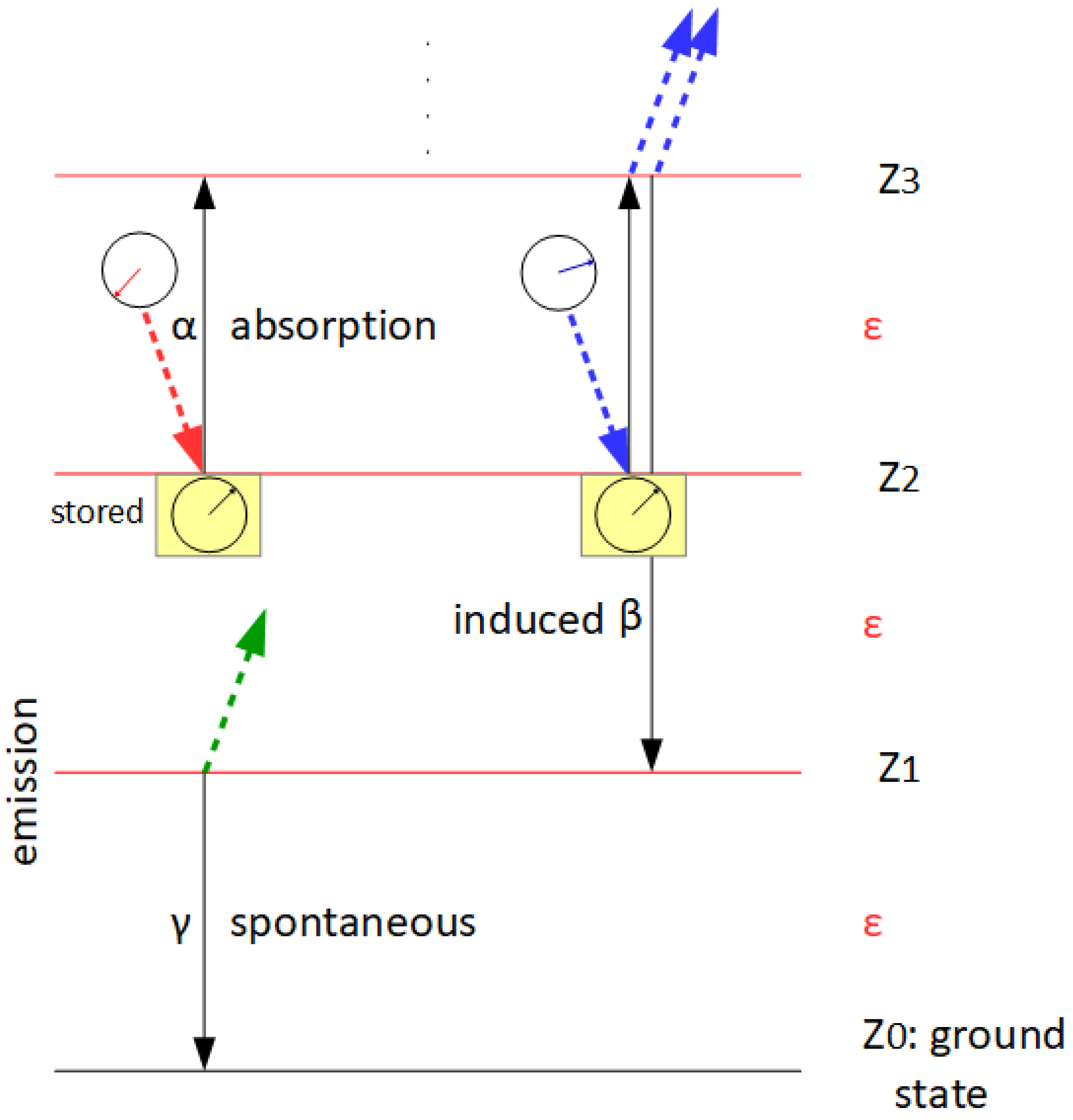
Figure 2. Boltzmann distribution (yellow) for one million molecules and the same number of quanta (left) or five times as many quanta (right). White: Poisson distribution with the same parameters. The red curve shows how the quanta are distributed among the molecules as a result of a Monte Carlo simulation when one quantum after the other is assigned to a randomly selected molecule. The two curves (red and white) are drawn slightly offset from each other, as otherwise one of the curves would completely obscure the other.

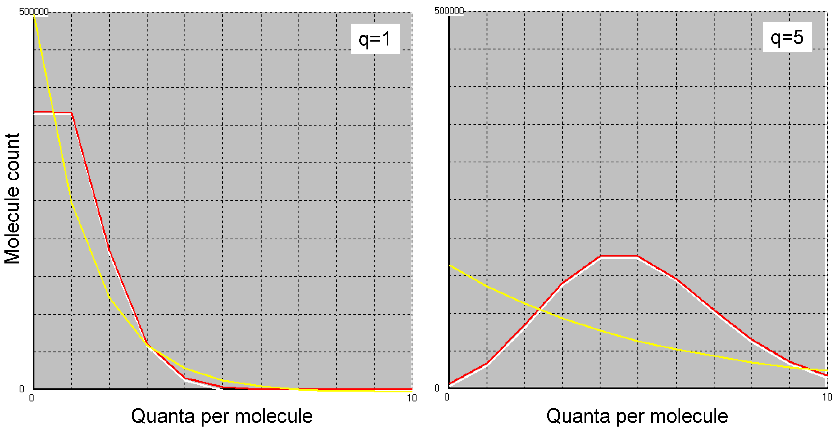
Figure 3. Comparison of the monochromatic two-state molecule (A) for the interaction of light with matter (according to R. Feynman, modified [10]), which can only be at two energy levels, with the monochromatic resonator (B) discussed here, in which any number of equidistant levels are possible. In B, absorption and induced emission can originate from the same level and can therefore be alternative events; this is not possible in A.

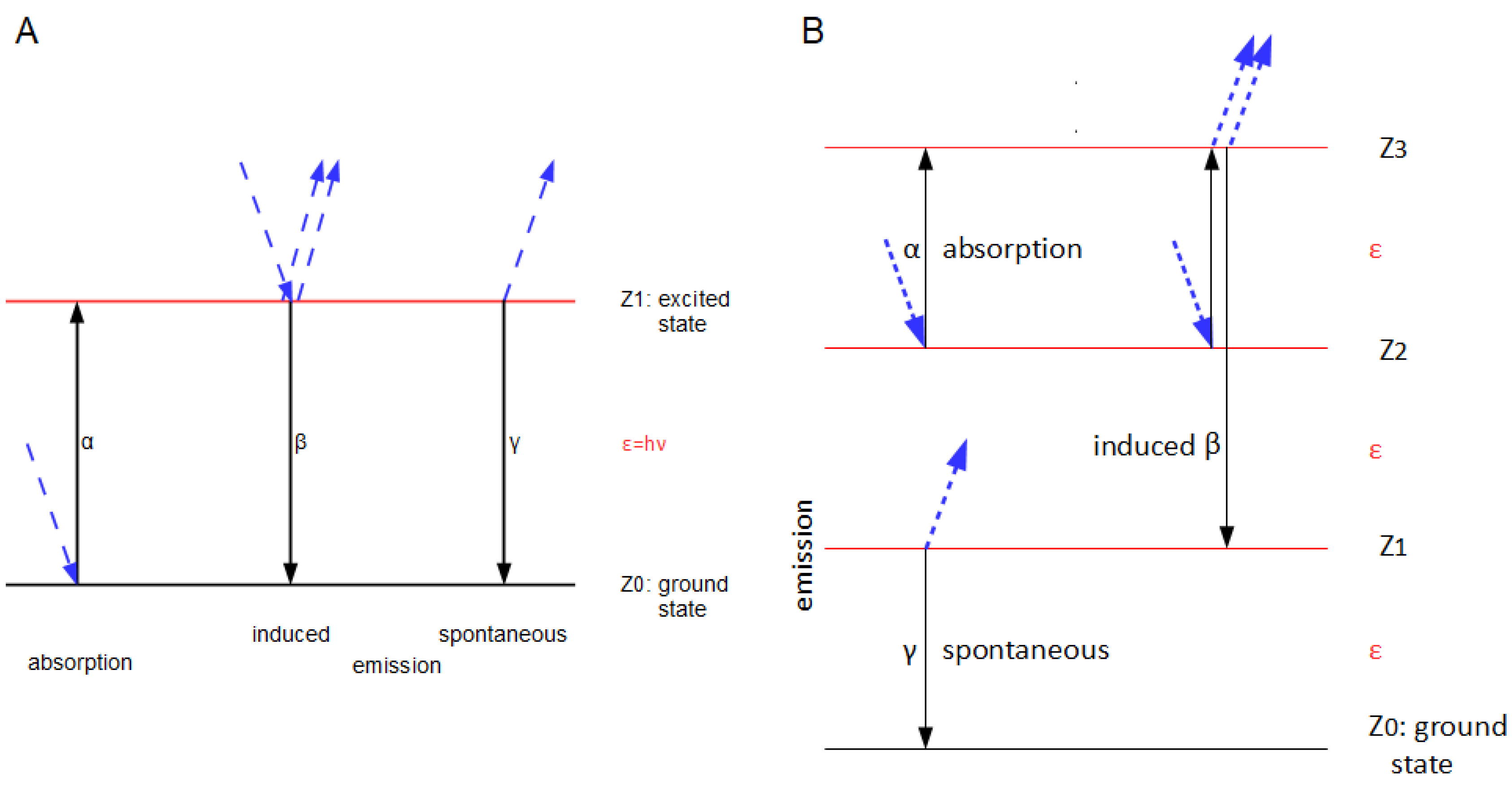
Figure 4. State distribution for one million resonators and as many (left) or five times as many (right) quanta (blue curve according to Eqs. 5.7 and 5.8, assuming δ=1). It was postulated that a quantum reservoir independent of the resonators exists. The yellow curve shows how the quanta are distributed among the resonators as a result of a Monte Carlo simulation in which the interactions between resonator and field were modelled as described in Figure 3. α=β=γ/2; δ=1. The two curves are drawn slightly offset from each other, as otherwise one of the curves would completely obscure the other.

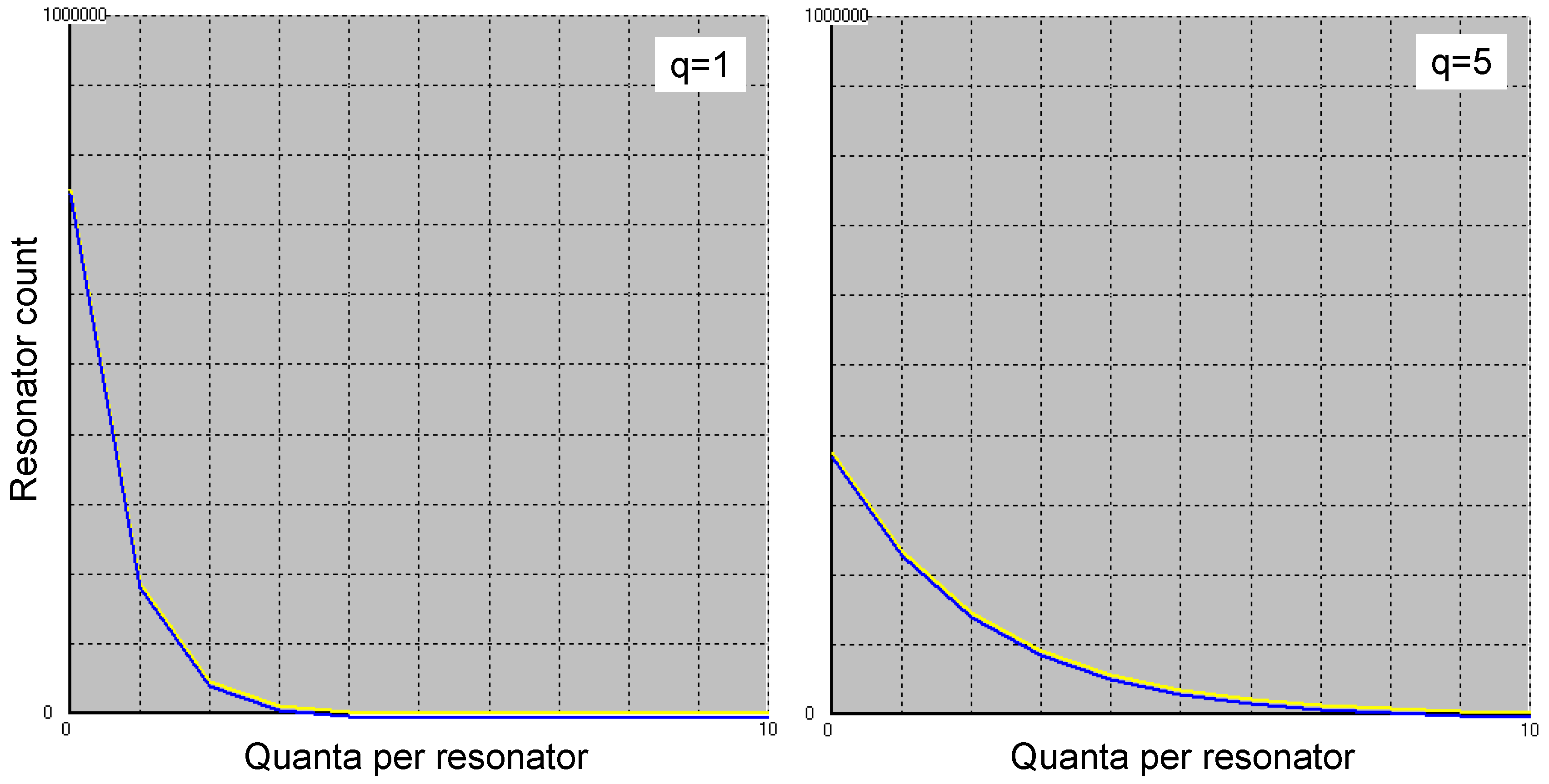
Table 1. Energy states of the dichromatic molecule (two-state system).

		ε
		Z₀	Z₁
aε	Z₀	n₀₀=(1-q_ε)(1-q_aε)	n₁₀=q_ε(1-q_aε)
aε	Z₁	n₀₁=(1-q_ε)q_aε	n₁₁=q_εq_aε

Disclaimer/Publisher’s Note: The statements, opinions and data contained in all publications are solely those of the individual author(s) and contributor(s) and not of MDPI and/or the editor(s). MDPI and/or the editor(s) disclaim responsibility for any injury to people or property resulting from any ideas, methods, instructions or products referred to in the content.

© 2025 by the authors. Licensee MDPI, Basel, Switzerland. This article is an open access article distributed under the terms and conditions of the Creative Commons Attribution (CC BY) license (http://creativecommons.org/licenses/by/4.0/).

Copyright: This open access article is published under a Creative Commons CC BY 4.0 license, which permit the free download, distribution, and reuse, provided that the author and preprint are cited in any reuse.

The Monochromatic Resonator and the Interaction Between Light and Matter Under the Assumption That Photons Follow Classical Trajectories

Abstract

Keywords:

Subject:

Introduction

References

MDPI Initiatives

Important Links

Subscribe