Vancouver Weather Dynamics Analysis: 2009-2019 Using Quantum Information Theory

1. Introduction

In recent years, the climate lost regularity in cycles and became changeable to new states [1]. The climate changes occupied big areas with totally or partially damaging ecosystems [2]. Human societies must deal the climate problem with the slightest responsibility in order to protect the earth from negative changes [3].

Over the past two years, the heat dome has swept away, causing high temperatures and low humidity, accompanied by a lack of rainfall in the north of the Earth during the summers of 2022 and 2023, sparking forest fires in Canada, America, Britain, and on both sides of the Mediterranean in Spain, France, Italy, Greece, Turkey, Morocco, Algeria, and Tunisia. In Greenland, glaciers are melting rapidly. Summer continues for more weeks, autumn shortens, and winter progresses slowly and ends early, paving the way for spring to return quickly. The melting of ice and the separation of huge areas of it in Antarctica. The hurricanesanes increased, approaching 300 km/h, and became more ferocious and violent. There are many examples that cannot be enumerated here of the dire consequences that the Earth is currently witnessing in terms of climate change over the past two years. The suffering of human societies has increased around the world in the face of extreme climate. Difficult challenges have emerged, particularly water availability, due to disturbances in rainfall and the impact of extreme temperatures on agriculture. The environment became unhealthy due to human manipulation [4].

In this context, researchers from all over the world have rushed to study the climate changes in each region and their repercussions on the social and economic systems of human societies in developed and developing countries [5,6,7,8]. They made good efforts and distinguished contributions. They invented more effective devices to measure the weather in order to obtain accurate data about climate phenomena. They then established mathematical models describing various climate phenomena. Hence, they developed statistical, numerical and analytical methods in treating weather data and linked them to human activities to understand the repercussions of climate change [9,10,11].

In developing statistical, numerical, and analytical studies of various weather phenomena, there was, on the other hand, a new theory that began to become famous. Almost thirty years ago, the new theory about information systems was suggested as the quantum information theory. Its primary purpose was to build and operate a quantum computer. This theory developed in a parallel way and far from the issue of climate change in the world. With the spread of the issue of climate change, we were keen to develop techniques to understand the climate, so we sought the quantum information theory as a new mathematical method in studying weather data in addition to other methods currently used. The purpose here is to provide a new perspective in the study of climate variables and the interaction between them. There are quantum measures that are suitable for studying the climate.

In this manuscript we will investigate the Vancouver weather dynamics in the time domain from 2009 to 2019 by the aid of quantum mechanical measurements. The manuscript is arranged as follows; in section two we introduce the framework of the measurement technique and the preparing of the data to be suitable for it and we deduce the density matrix of the quantum system. In section three, we obtain the time evolution of the classical information, the quantum information, the decoherent information, Shannon entropy and von Neumann entropy monthly. Also, we recorded the maximum values of each case. In section four, we end with the conclusion.

2. The Mathematical Model

The novelty of this framework is configured to set up the quantum machine learning (QML) as the $d-$dimensional feature space F, of the dataset $\mathbb{X},$ in a viewpoit of the quantum information theory. Thus, we aim to formulate the dataset $\mathbb{X},$ in the quantum view. In the classical information system, the dataset $\mathbb{X},$ is provided as $n\times d$ matrix where n and d refers to the number of rows and number of columns respectively where $x_{ij}$ is the numerical value in the dataset $\mathbb{X},$$i=1,2,3,...,n,$ and $j=1,2,3,...,d$. Therefore, the $d-$dimensional feature space F, is represented geometrically by the Hilbert space in the quantum framework where each feature represents a specific phenomenon provided in the standard basis vector. Consequently, the $d-$dimensional feature space F, is configured by standard bases $\left|c_1\right.〉,\left|c_2\right.〉,...,\left|c_d\right.〉$ where each column of $\mathbb{X}$ is represented by the standard basis and each row of $\mathbb{X}$ is formed by an arbitrary non-normalized vector $\left|r_i\right.〉,$$i=1,2,3,...,n.$ Hence, an arbitrary non-normalized vector $\left|r_i\right.〉$ can be formed in terms of the standard bases $\left|c_1\right.〉,\left|c_2\right.〉,...,\left|c_d\right.〉$ as:

$$\left|r_i\right.〉=\sum _{j=1}^d{x}_{ij}\left|c_j\right.〉,$$

(1)

Hence, the vector $\left|r_i\right.〉$ is normalized if it is taken in the form $\left|R_i\right.〉$ as follows:

$$\left|R_i\right.〉=\sum _{j=1}^d{r}_{ij}\left|c_j\right.〉,$$

(2)

where $r_{ij}=x_{ij}/\sqrt{{\sum }_{j=1}^d{\left|x_{ij}\right|}^2}$ such that ${\sum }_{j=1}^d{\left|r_{ij}\right|}^2=1.$ A given dataset $\mathbb{X}$, is defined on the set of real numbers $\mathbb{R}$ or the set of complex numbers $\mathbb{C}$ according to domains of $x_{ij}$’s elements. Indeed, the dataset $\mathbb{X}$, cannot be treated in the quantum mechanics, since it is not a square matrix. In this respect, the new quantum state $\rho ,$ is defined to describe $\mathbb{X}$, provided by the square matrix. The quantum state $\rho ,$ is the normailzed square matrix of order $d\times d,$ and is introduced as:

$$\rho :={\displaystyle \frac{{\mathbb{X}}^T\mathbb{X}}{tr\left({\mathbb{X}}^T\mathbb{X}\right)}}.$$

(3)

which expressed in terms of standard bases $\left|c_1\right.〉,\left|c_2\right.〉,...,\left|c_d\right.〉$ as follows:

$$\rho =\sum _{i,j=1}^d{\rho }_{ij}\left|c_i\right.〉\left.〈c_j\right|.$$

(4)

where ${\sum }_{i=1}^d{\rho }_{ii}=1.$ The state $\rho$ has three important facts. Firstly, it is always a mixed state. Hence, it has always a noise. Diagonal elements ${\rho }_{11},{\rho }_{22},...,{\rho }_{dd}$ represent the classical information denoted by $CI$. $CI$ is the information that can be directly observed, stored, and processed using traditional digital technologies. $CI$ is investigated by:

$$CI=\sum _{n=1}^d{\rho }_n^2.$$

(5)

Non-diagonal elements ${\rho }_{ij};i\ne j,$ are the joint information of ket basis $\left|c_i\right.〉$ and bra basis $\left.〈c_j\right|,$ which describes the quantum information. These elements disappear in the classical information but exist in the quantum information theory. Hence, the quantum information theory forms a new type of the information which does not exist classically. $QI$ is fundamentally different from $CI$ which is due to the unique properties of quantum systems, such as superposition. $QI$ is checked by:

$$QI=2\sum _{n=d+1}^{d\left(d-1\right)/2}{\left|{\rho }_n\right|}^2.$$

(6)

Clearly, two informaation terms CI and QI, yield the trace of ${\rho }^2$ which is written as:

$$Tr{\rho }^2=CI+QI.$$

(7)

Hence, the new term is also defined as $1-Tr{\rho }^2,$ and is known as the linear entropy or purity. Here this term is named the decoherent information and denoted by $DI$. $DI$ refers to the private information type that is not directly accessible or measurable with matrix elements like $CI$ and $QI.$$DI$ is detected by the relationship as:

$$DI=1-Tr{\rho }^2.$$

(8)

If $\rho$ is the pure state, then the sum of $CI$ and $QI$ is equal to one and $DI$ does not exist. Thus, Equation (7) becomes as follows:

$$CI+QI=1.$$

(9)

If $\rho$ is the mixed state, then the sum of $CI$ and $QI$ is less than one and there is a gap which forms the inequality in Equations (7) and (9). Therefore, a new term achieves the equality in the preceded inequality. $DI$ describes a gap between one and the sum of $CI$ and $DI$ with using Equation (8) in what follows:

$$CI+QI+DI=1.$$

(10)

The information has distinct realms, each with its own unique characteristics, and through which we can understand systems. The quantum information system can be divided into three different categories; $CI$, $QI$, and $DI$. According to the quantum informative view, the dataset $\mathbb{X}$, is manipulated by the formation of $\rho ,$ over the $d-$dimensional feature space F. Consequently, the quantum machine learning is defined here successfully.

To study the noise and the ambiguity of the information system, the entropy is used here to handle this mission. Indeed, the entropy is valid to measure the noise with a high accuracy. Shannon entropy is used to determine the noise of the classical information and is introduced as [12]:

$$S_H=-\sum _i^d{\rho }_i{log}_d{\rho }_i.$$

(11)

where $S_H>0,$ and depends on the diagonal terms of $\rho .$$S_H$ always exists for all cases of $\rho .$ von Neumann entropy is a precise and widely-used quantum measure due to its strong theoretical foundations and it is also known as nonlinear entropy. It is a quantum analogues of the classical Shannon entropy and is introduced as [13]:

$$S_N=-\sum _i^d{\lambda }_i{log}_d{\lambda }_i$$

(12)

where ${\lambda }_i$ is the eigenvalue of the quantum state $\rho$. von Neumann entropy can be applied to any quantum state, whether pure or mixed, and is not limited to particular systems or states. This makes it a versatile and widely applicable quantum measure. Consequently, $S_N=0,$ if $\rho$ is a pure state and $S_N>0,$ if $\rho$ is a mixed state. Hence, $S_N$ measures the noise of the decoherent information.

3. Quantum Weather Model

In this setting, we propose this novel technique to investigate the weather dynamics in Canada as a good exercise. Climate changes in Canada are in the spotlight here. Canada characterizes a wide range of both of geological and meteorological regions. It has a cold continental climate with winters lasting for six months and heavy snow falls, covering vast areas. In addition, the rainfall falls with great annular rates over all provinces and territories. Temperatures vary in the summer from a region to a region [14,15,16,17]. Thus, no one can study totally the climate in Canada. Therefore, the study is focused on a local region like Vancouver city. Some of basic information is provided about the geography and the climate of Vancouver city. Vancouver is a major city in western Canada, located in the Lower Mainland region of British Columbia province. It lies between Burrard Inlet to the north and the Fraser River to the south. The Strait of Georgia, to the west, is shielded from the Pacific Ocean by Vancouver Island. It is one of Canada’s warmest cities in the winter. Vancouver’s climate is temperate by Canadian standards and is marine west coast. In the summer, it is dry [18].

Vancouver weather dataset is investigated by the weather dataset as an example for the QML. The dataset is formed of ten weather variables and 4017 records from on January 2009 to 31^th December 2019 [19]. Here, names of weather variables are the maximum temperature (K), the minimum temperature (K), the dew point (K) where K is Keliven, the cloudcover (%), the humidity (%), the precipitation (mm), the total Snow (cm), the pressure (bar), the wind direction degree, and the wind speed (km/h) respectively.

In this setting, consider the quantum ten-dimensional feature space of bases $\left|c_1\right.〉,$$\left|c_2\right.〉,$$...,$ and $\left|c_{10}\right.〉,$ to represent the weather model with this novel technique. Weather vraiables are formulated in the quantum ten-dimensional feature space as the maximum temperature $\left|c_1\right.〉$, the minimum temperature $\left|c_2\right.〉$, the dew point $\left|c_3\right.〉$, the cloudcover $\left|c_4\right.〉$, the humidity $\left|c_5\right.〉$, the precipitation $\left|c_6\right.〉$, the total Snow $\left|c_7\right.〉$, the pressure $\left|c_8\right.〉$, the $x-$wind speed $\left|c_9\right.〉,$ and the $y-$wind speed $\left|c_{10}\right.〉,$ where the wind speed and the wind direction are solved into the $x-$wind speed and the $y-$wind speed respectively.

Thus, an arbitrary instance pure weather state $\left|w_i\right.〉$ gives the numerical data of the $i-$row in the weather dataset $\mathbb{W}$ and can be written as:

$$\left|w_i\right.〉=\sum _{j=1}^{10}{w}_{ij}\left|c_j\right.〉.$$

(13)

where $w_{ij}$’s are real values. The daily quantum weather state is symbolized as $\left|d,m,y\right.〉$ where d is the day order in the month, m is the month order, and y is the year. If the date is 03/01/2009, then the corresponding daily quantum weather state of the same date is written as $\left|03,01,2009\right.〉.$ Consequently with using Equations (1) and (13), the quantum daily weather state $\left|03,01,2009\right.〉$ can be described by a numerical data in terms of ten bases as follows:

$$\begin{array}{ccc}\hfill \left|03,01,2009\right.〉& =& 275\left|c_1\right.〉+271\left|c_2\right.〉+272\left|c_3\right.〉+82\left|c_4\right.〉+96\left|c_5\right.〉\hfill \\ & & +2.2\left|c_6\right.〉+0.8\left|c_7\right.〉+1021\left|c_8\right.〉-6.35\left|c_9\right.〉+12.47\left|c_{10}\right.〉\hfill \end{array}$$

(14)

where the state $\left|03,01,2009\right.〉$ gives the data record in Vancouver weather dataset.

It is obvious that the daily quantum weather state is unbalance because of all data have distinct units. Therefore, it necessary that all data is reformed in dimensionless data in order to be balanced. To achieve this aim, the maximum reference of each column is calculated from $01/01/2009$ to $31/12/2019$ in the Vancouver weather dataset on the data in Table 1. In the maximum reference (Max- Ref) approach, the daily quantum weather state $\left|03,01,2009\right.〉$ can be reformed in dimensionless data where each value of a weather variable is divided by the corresponding maximum reference value of the same weather variable as in Table 1, in what follows:

$$\begin{array}{ccc}{\left|03,01,2009\right.〉}_{Max\_Ref}& =& 0.9136\left|c_1\right.〉+0.9217\left|c_2\right.〉+0.9347\left|c_3\right.〉+0.82\left|c_4\right.〉+0.9697\left|c_5\right.〉\hfill \\ & & +0.0279\left|c_6\right.〉+0.0976\left|c_7\right.〉+0.9779\left|c_8\right.〉-0.1765\left|c_9\right.〉+0.3465\left|c_{10}\right.〉\hfill \\ \hfill \end{array}$$

(15)

where Equation (15) is non-normalized. In subsequent by Equation (2), the state ${\left|03,01,2009\right.〉}_{Max\_Ref}$ becomes normalized as:

$$\begin{array}{ccc}\hfill {\left|03,01,2009\right.〉}_{Max\_Ref\_N}& =& 0.3973\left|c_1\right.〉+0.4008\left|c_2\right.〉+0.4064\left|c_3\right.〉+0.3566\left|c_4\right.〉+0.4217\left|c_5\right.〉\hfill \\ & & +0.0122\left|c_6\right.〉+0.0424\left|c_7\right.〉+0.4253\left|c_8\right.〉-0.0768\left|c_9\right.〉+0.1507\left|c_{10}\right.〉\hfill \\ \hfill \end{array}$$

(16)

Actually, the daily quantum weather state ${\left|03,01,2009\right.〉}_{Max\_Ref\_N}$ is pure normalized. Each numerical value of dimensionaless weather variable is affected by other values of all variables using the normailzation constant. All same computations are established over all instance weather states in this statistics to obtain normalized quantum pure daily weather states. According to the statistics, we have 4017 normalized daily quantum pure weather states from $01/01/2009$ to $31/12/2019$.

How to construct the state $\rho$ over an arbitrary date interval from the $i-$row to the $j-$row, the first step, the weather dataset $\mathbb{W},$ is modified into a new formalism which each column is divided by the corresponding maximum reference according to Table 1. Thus, the new dimensionless weather dataset $\mathbb{S}$ is built. The second step, the state $\rho \left(i:j\right)$ from the $i-$row to the $j-$ row is computed by Equation (3) as:

$$\rho \left(i:j\right)={\displaystyle \frac{{\mathbb{S}}^T\left(i:j\right)\mathbb{S}\left(i:j\right)}{tr\left({\mathbb{S}}^T\left(i:j\right)\mathbb{S}\left(i:j\right)\right)}}.$$

(17)

This statistics is partitioned according to months. Thus, there are 132 covariance matrices $\mathbb{S}\left(1:31\right),$$\mathbb{S}\left(32:59\right),$ ...,$\mathbb{S}\left(3957:3986\right),$ and $\mathbb{S}\left(3987:4017\right),$ which correspond to $1/2009,2/2009,...,11/2019$, and $12/2019$, respectively. The monthly quantum state $\rho \left(1/2009\right)$ is determined from $01/01/2009$ to $31/12/2009$, by Equation (17):

$$\rho \left(1/2009\right)={\displaystyle \frac{{\mathbb{S}}^T\left(1:31\right)\mathbb{S}\left(1:31\right)}{tr\left({\mathbb{S}}^T\left(1:31\right)\mathbb{S}\left(1:31\right)\right)}}.$$

(18)

and the corresponding matrix of $1/2009$ is computed as:

$$\begin{array}{ccc}& & \rho \left(1/2009\right)=\hfill \\ & & \left[\begin{array}{cccccccccc}0.1780& 0.1798& 0.1816& 0.0950& 0.1633& 0.0058& 0.0071& 0.1894& -0.0162& 0.0225\\ 0.1798& 0.1817& 0.1835& 0.0963& 0.1651& 0.0059& 0.0072& 0.1914& -0.0165& 0.0227\\ 0.1816& 0.1835& 0.1853& 0.0974& 0.1669& 0.0060& 0.0073& 0.1933& -0.0167& 0.0228\\ 0.0950& 0.0963& 0.0974& 0.0764& 0.0943& 0.0059& 0.0072& 0.1010& -0.0157& 0.0148\\ 0.1633& 0.1651& 0.1669& 0.0943& 0.1532& 0.0061& 0.0074& 0.1737& -0.0175& 0.0198\\ 0.0058& 0.0059& 0.0060& 0.0059& 0.0061& 0.0008& 0.0008& 0.0061& -0.0017& 0.0015\\ 0.0071& 0.0072& 0.0073& 0.0072& 0.0074& 0.0008& 0.0056& 0.0075& -0.0021& 0.0036\\ 0.1894& 0.1914& 0.1933& 0.1010& 0.1737& 0.0061& 0.0075& 0.2016& -0.0171& 0.0240\\ -0.0162& -0.0165& -0.0167& -0.0157& -0.0175& -0.0017& -0.0021& -0.0171& 0.0059& -0.0027\\ 0.0225& 0.0227& 0.0228& 0.0148& 0.0198& 0.0015& 0.0036& 0.0240& -0.0027& 0.0114\end{array}\right].\hfill \end{array}$$

(19)

Elements of the state $\rho \left(1/2009\right)$ expresses for the classical information which appear in diagonal elements and the quantum information which appear in non-diagonal elements. In fact, each element matrix is influenced by all weather dimensionaless variables because of the term $tr\left(S^T\left(1:31\right)S\left(1:31\right)\right).$ Vancouver ether dataset is checked later by quantum informative measurements (the classical information, the quantum information, the decoherent information, Shannon entropy and von Neumann entropy).

4. Discussion and Results

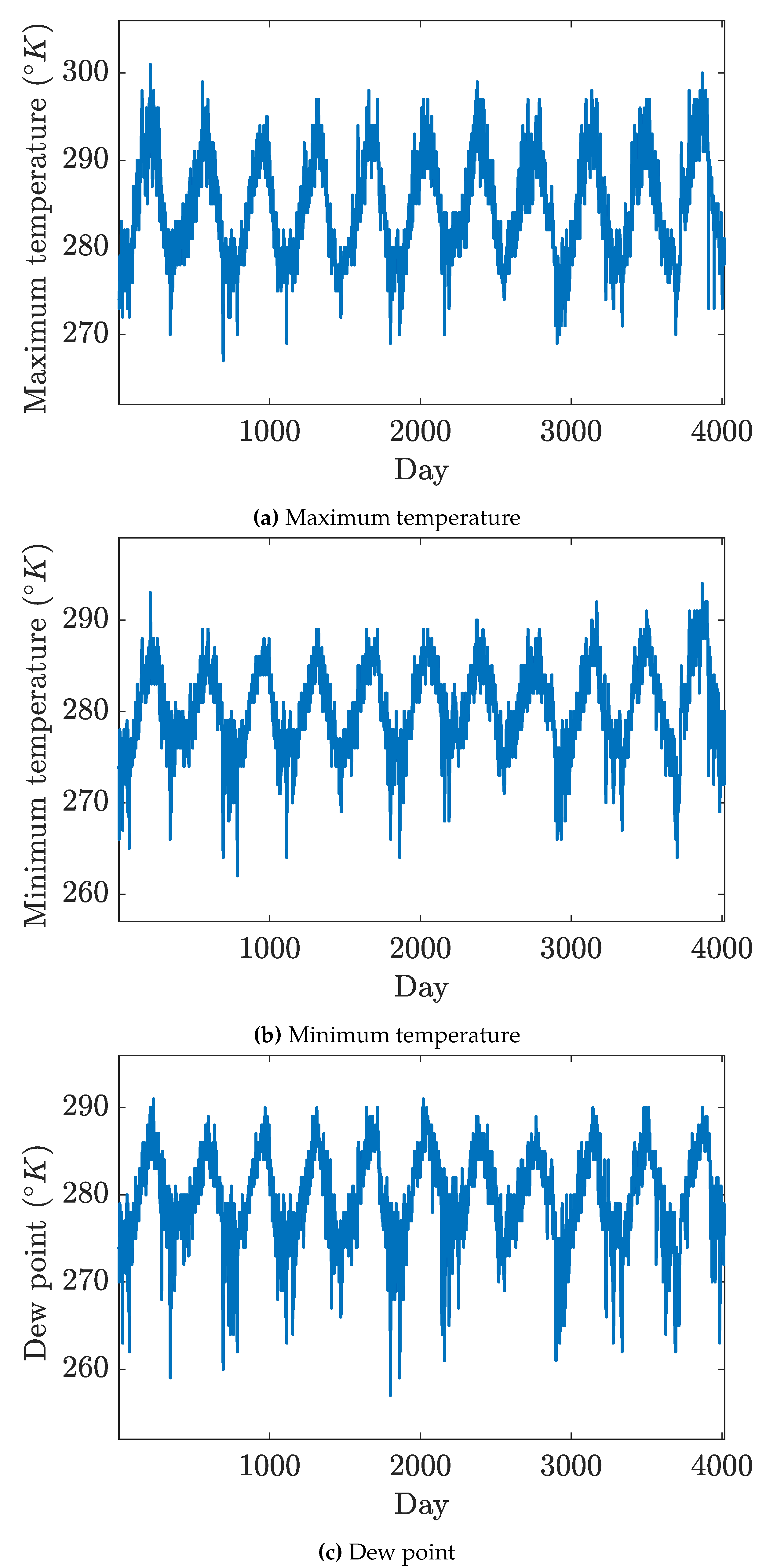
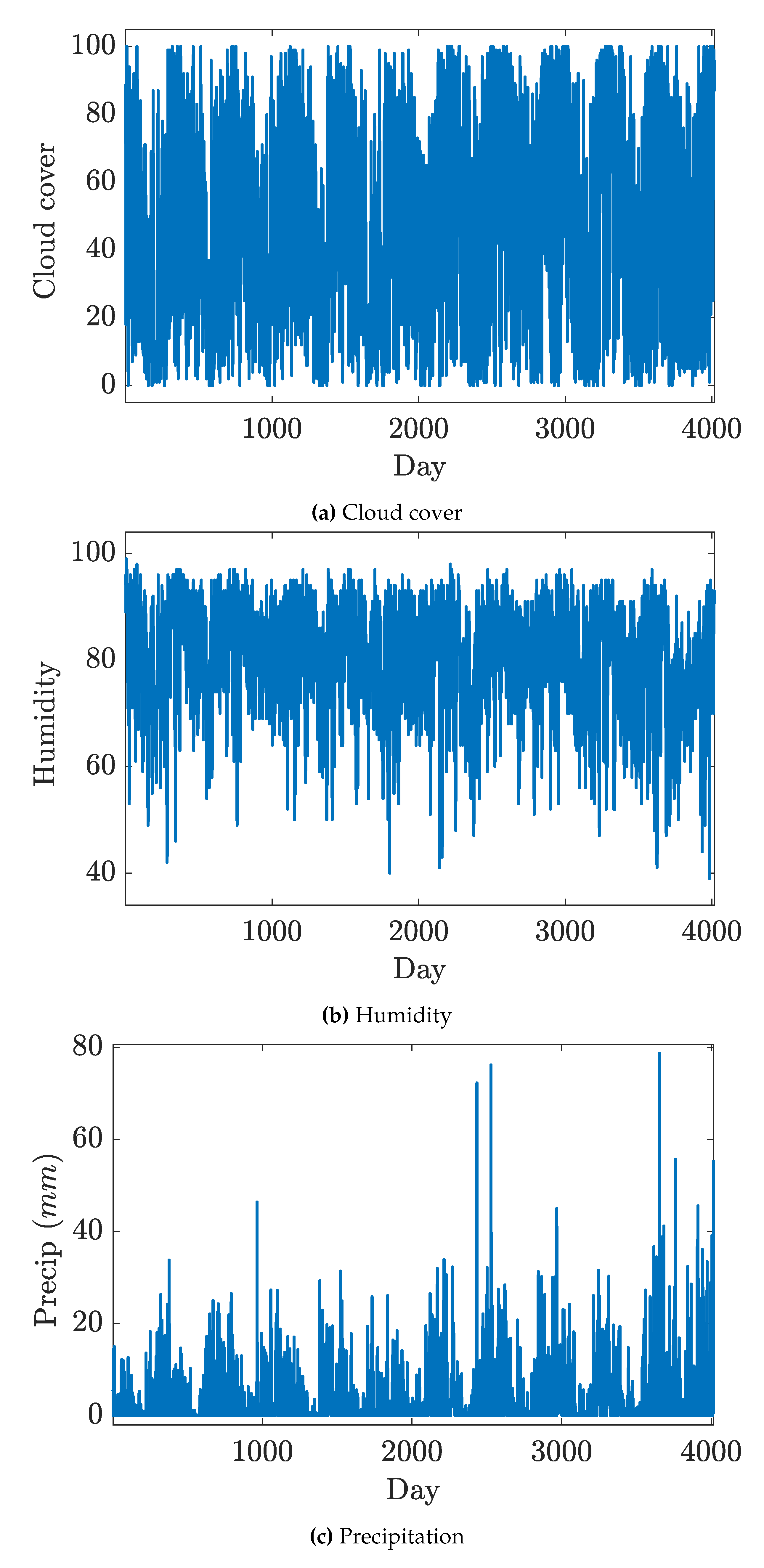
In order to study the climate, one needs to visualize the time evolution of the climate variables and we can get a comprehensive understanding of each one of them. This allows us to detect extremes, trends, and the overall climate characteristics. Figure 1, shows the time evolution of each climate variable. Figure 1 and Figure 1, presents the evolution of the maximum temperature, minimum temperature, and dew point in Keliven. It is clear that we have a cyclic evolution yearly, whereas the maximum of each cycle is reached in the half of each year and the minimum is recorded at the beginning and the end of each year. Indeed, the cloud cover and humidity percentage have no cyclic evolution as shown in Figure 2,Figure 2. If we look insight, we can detect a trend of increase in the maximum precipitation values with an extreme values in 2015 as shown in Figure 2. 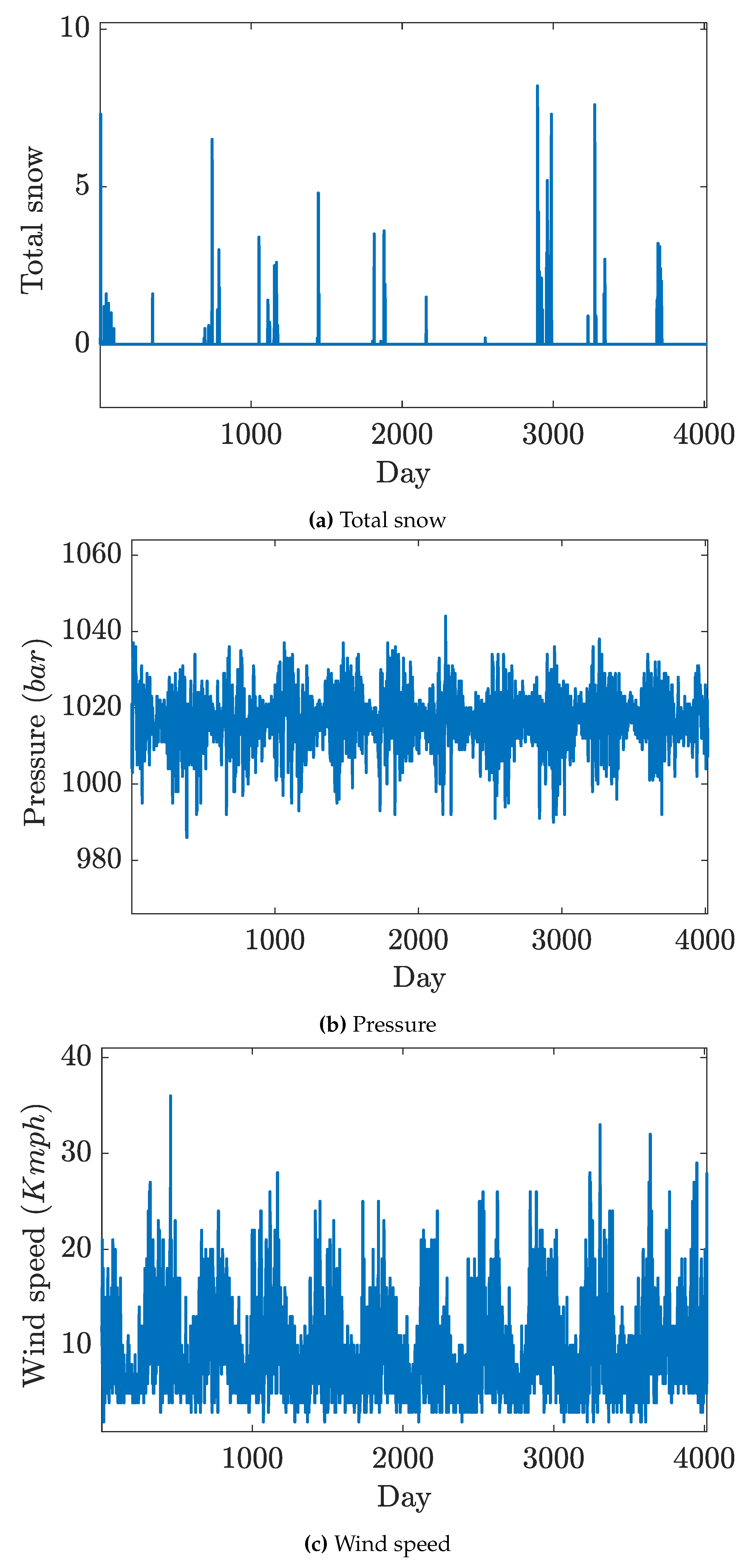Figure 3 presents a roughly oscillation without any cyclic evolution whereas the mean values are approximately constant. Snow is a discrete time phenomena happening per year, so as in Figure 3, total snow is recorded in between sequential two years. Indeed the total snow has its extreme in 2016 and 2017. In Figure 3, wind speed has a cyclic evolution with fluctuations in each year. Also, the minimum value are approximately stationary with respect to the variation in the maximum values.

In this analysis of a time evolution in the feature space, the classical information CI, the quantum information QI, the decoherent information DI, Shannon entropy and von Neumann entropy are plotted against the months as the time units from Jan/2009 into Dec/2021. Information has distinct realms, each with its own unique characteristics, and through which we can understand systems.

The classical information, the quantum information, the decoherent information, Shannon entropy and von Neumann entropy are computed for monthly mixed states by Equations (5), (6), (8), (11), (12), (17), (18), (19), and all numerical values are mentioned in tables. Table 2, Table 3, Table 4, Table 5 and Table 6 refer to the classical information, the quantum information, the decoherent information, Shannon entropy and von Neumann entropy rerspcetively. Each table includes 132 numerical values refers to years from 2009 to 2019 vertically and to months horizontally from January to December.

In Table 2, values of CI provide the effect individually of each weather variable of a range $\left[0.1567,0.2012\right].$ In Table 3, values of QI describe the mutual interaction of pair of two variables of a range $\left[0.7296,0.8023\right]$. Obviously, QI values enlarge comparison with values of CI. Therefore, the effect of QI is greater than the effect of CI in this system. In Table 4, DI values are small relative to QI and CI and has a range $\left[0.0090,0.0882\right]$. In Table 5, $S_H$ values describe the classical noise of CI and is ranged by $\left[0.7201,0.8368\right].$ in Table 6, $S_N$ values describe the noise of DI of a range $\left[0.0147,0.1172\right]$. It noted that $S_N$ values weaken relative to $S_H$ values.

In order to predict quantum informative measures for proceeding years, the time evolution of quantum informative measures can be categorized by oscillating forms for the monthly evolution. We can adopt the time series function like Fourier series as a fitted function to express for quantum informative measures of the time t which takes the form:

$$f\left(t\right)=A_0+\sum _{n=1}^{10}(A_{n}cos\left({\displaystyle \frac{\pi }{12}}nt\right)+B_{n}cos\left({\displaystyle \frac{\pi }{12}}nt\right)).$$

(20)

where the time unit is the month and varies from 1 to 156 to express for years from 2009 to 2021. Also, $A_0,A_1,...,A_{10},B_1,B_2,...,B_{10}$ are real parameters which are detemined by the fitting curve method. The fitting curve method is applied from 2009 to 2017 where $t=1,2,...,108,$ and we compare predicated results with computational values in Table 2, Table 3, Table 4, Table 5 and Table 6 from 2018 and 2019, where $t=109,110,111,...,132$. Hence, we predict values for each quantum informative measure for 2020 and $2021,$ where $t=133,134,...,156.$ Parameters of Equation (20) are determined In Table 7 for $CI$, $QI$, $DI$, $S_H$ and $S_N$.

Table 8 presents a comprehensive analysis of the statistical parameters for predicted data CI, QI, DI, $S_H$, and $S_N$ based on data from 2009 to 2019. The parameters evaluated include maximum error $E_{max}$, average error $E_{avg},$minimum error $E_{min},$ standard deviation $\sigma$ and Pearson correlation $P.$ Among the models, CI demonstrates the lowest errors, with $E_{max}=0.0181$ and $E_{avg}=0.0044$, indicating more consistent predictions with minimal deviation. Conversely, Shannon entopy shows the highest errors, with $E_{max}=0.0437$ and $E_{avg}=0.0115$. The minimum error values across all models are in the range of ${10}^{-5}$ with CI having the lowest at $4.23068\times {10}^{-6}$and Shannon entropy the highest at $1.76316\times {10}^{-5}$. The standard deviation, which reflects the spread of prediction errors, is lowest for CI at 0.0036 and highest for S_Pred at 0.0092, reinforcing the observation that CI offers more stable predictions. In terms of performance accuracy, CI scores the highest with P at 0.8619, indicating superior reliability, while QI has the lowest accuracy at 0.4705. Overall, the table suggests that CI outperforms the other models in terms of error minimization and prediction accuracy, making it the most reliable among the five models analyzed.

In Table 9, all predicted values of each quantum informative measure are recorded from 2020 to 2021 based on months from $t=133,134,135,...,156.$

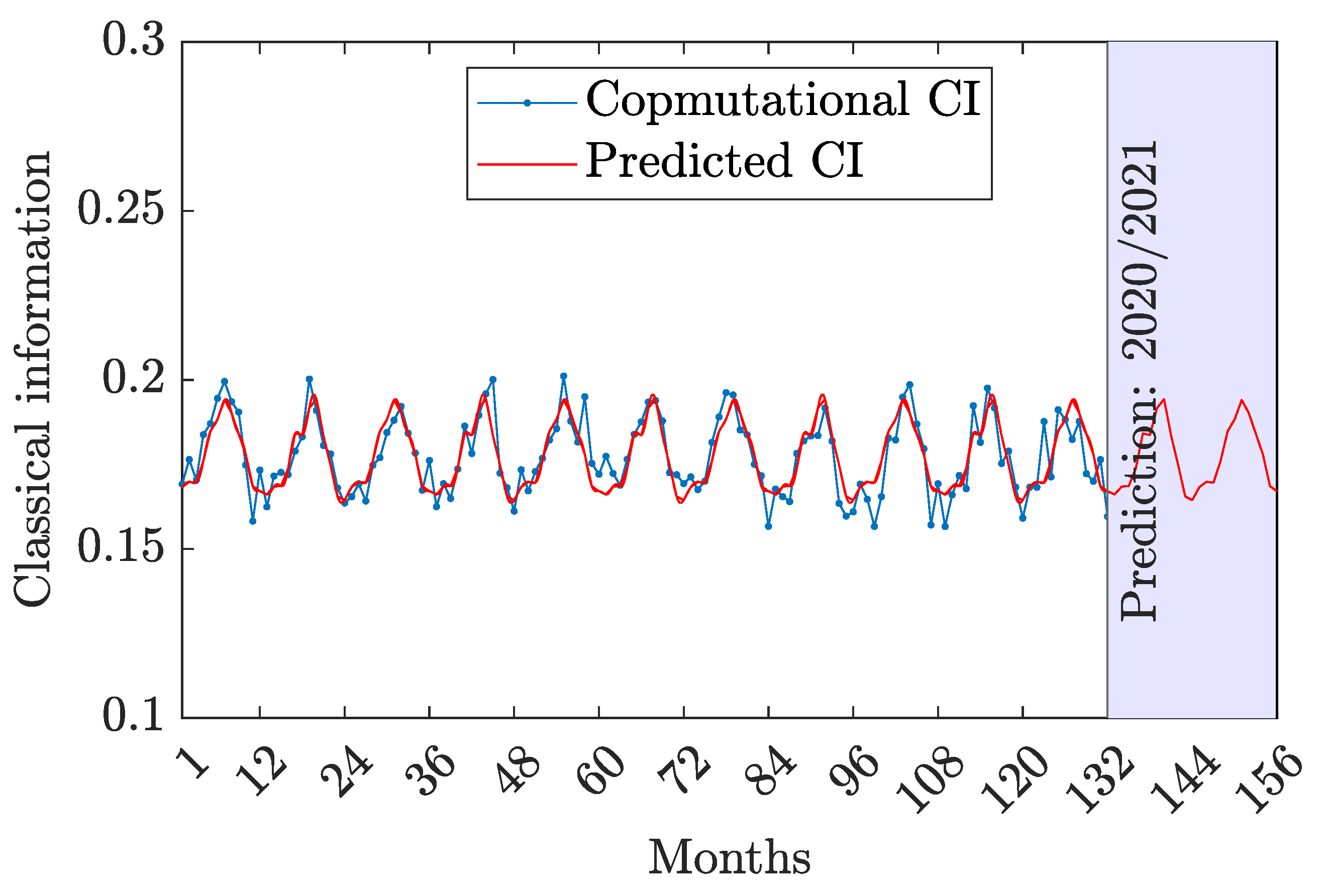
Each quantum informative measure investigates monthly mixed weather states. In all figures, each quantum informative measure is plotted versus the months as the unit time from 1 to 156 where the month domain $\left[1,132\right]$ provides the computational values and the month domain $\left[1,156\right]$ presents predicted values, especially future predicted values from 133 to 156. The blue curve represents computational values and the red curve shows predicted values. The shaded area on the right figure during the period $[133,156]$ marks the prediction period for 2020 and 2021. Predicated curves are plotted by Equation (20) and Tables (Table 7,Table 9). All curves are taken in waveforms.

Figure 4, Figure 5 and Figure 6 show a comparison between three distinct types of the information; CI, QI, and DI, respectively. In Figure 4, the classical information is plotted by Table 2, Table 7 and Table 8 and Equation (20) versus months in two curves. Two curves are close in nearly sinusoidal forms with a cyclic behavior. It has maximum extremes in summer and minimum in winter.

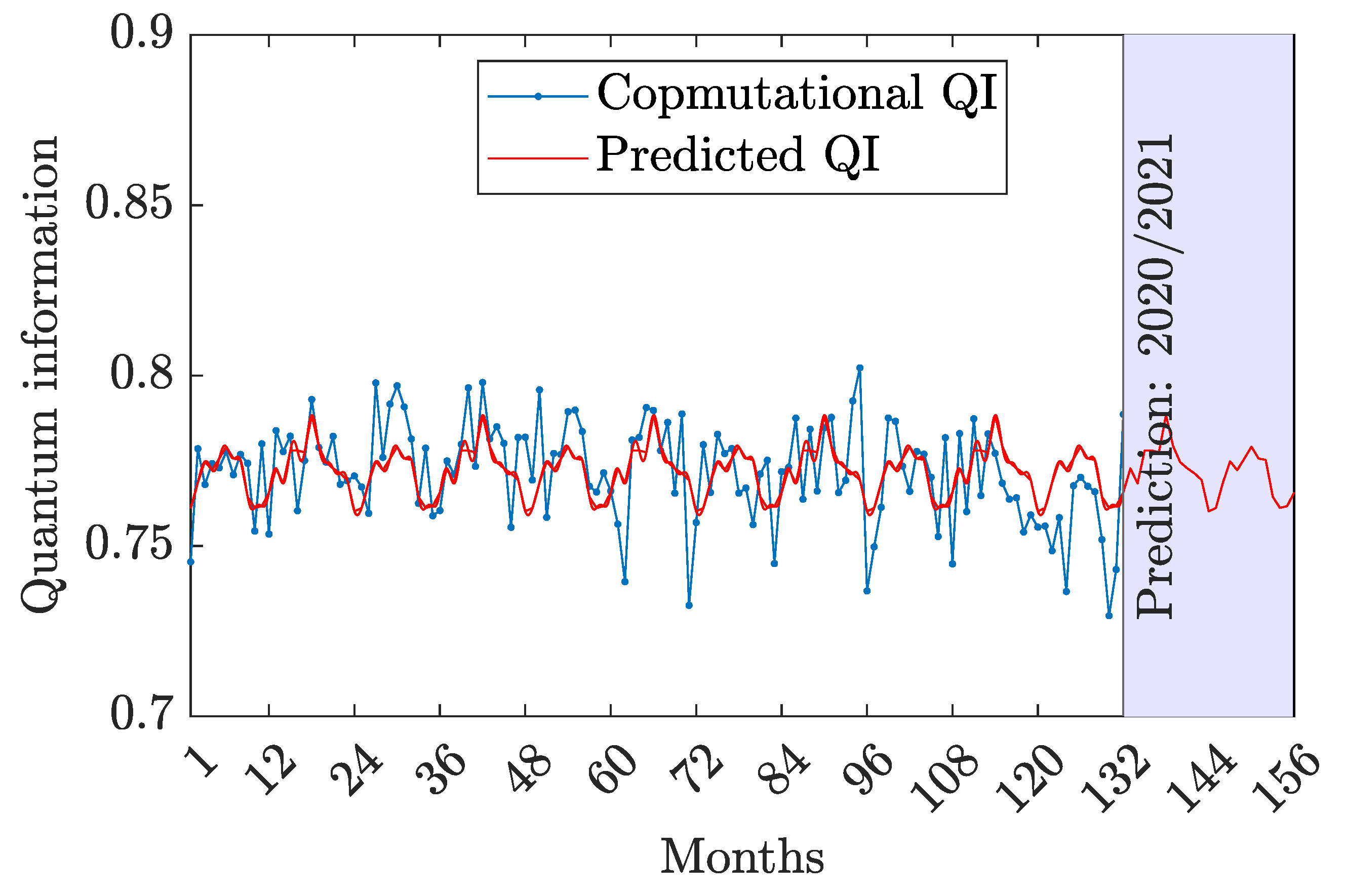
In Figure 5, by Table 3, Table 7 and Table 8 and Equation (20), the quantum information is plotted against months in two curves. The computational curve fluctuates far the predicted curve. The computational curve appears in an irregular behavior while the predicted curve has regular behavior. However, it depicts fluctuations in QI with no clear long-term increasing or decreasing trend.

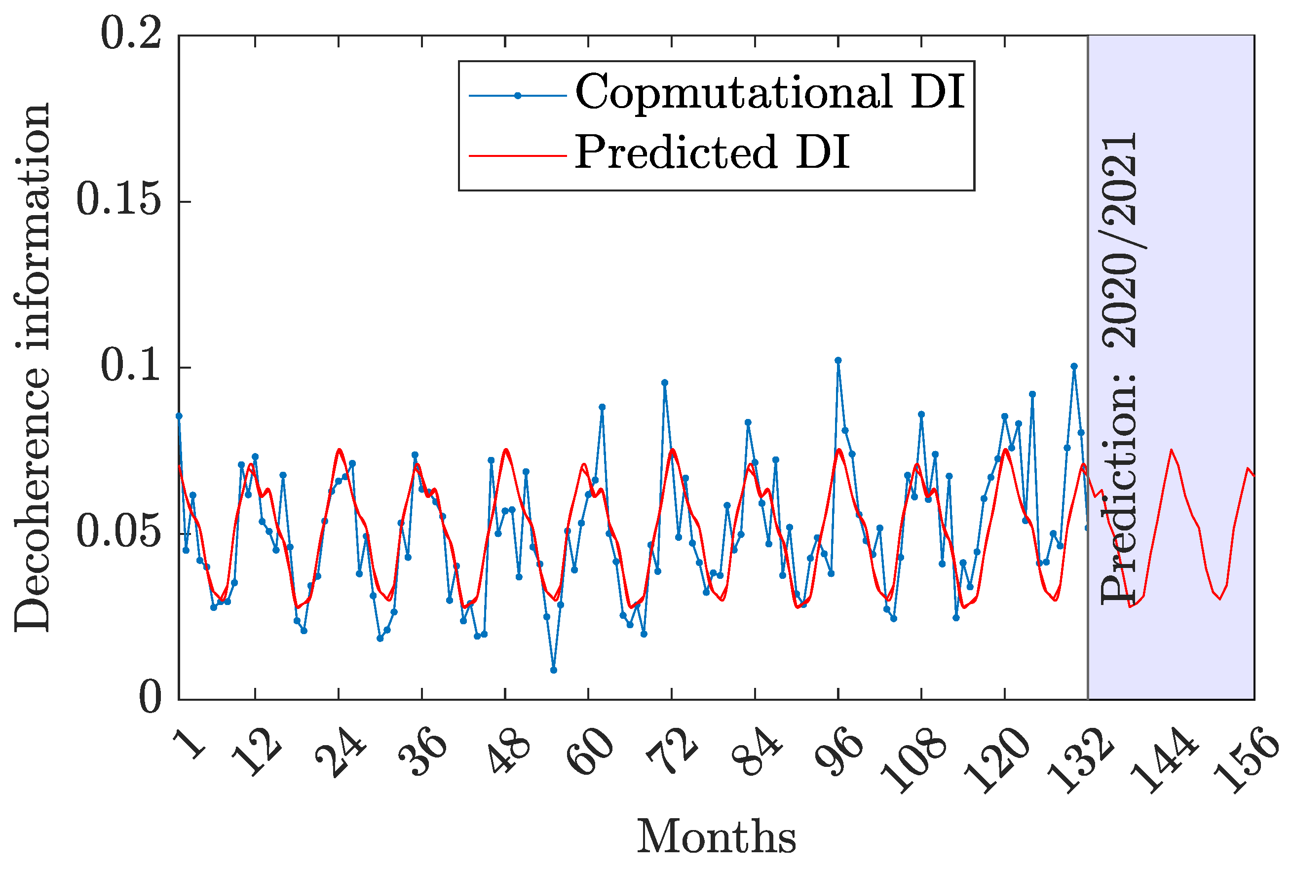
By Table 4,Table 7,Table 8 and Equation (20), the decoherent information is provided graphically versus months by two curves in Figure 6. The computational curve undergoes slight fluctuations but the predicated curve is regular. Indeed, the system exhibits a high value of the quantum information relative to the classical information which means that the model behaves like a real quantum model rather than a classical one. When the information measures are compared; QI exhibits the highest value with respect to CI and DI. This proves that a treatment of the quantum mechanical system will provide with considerable information with respect to classical one.

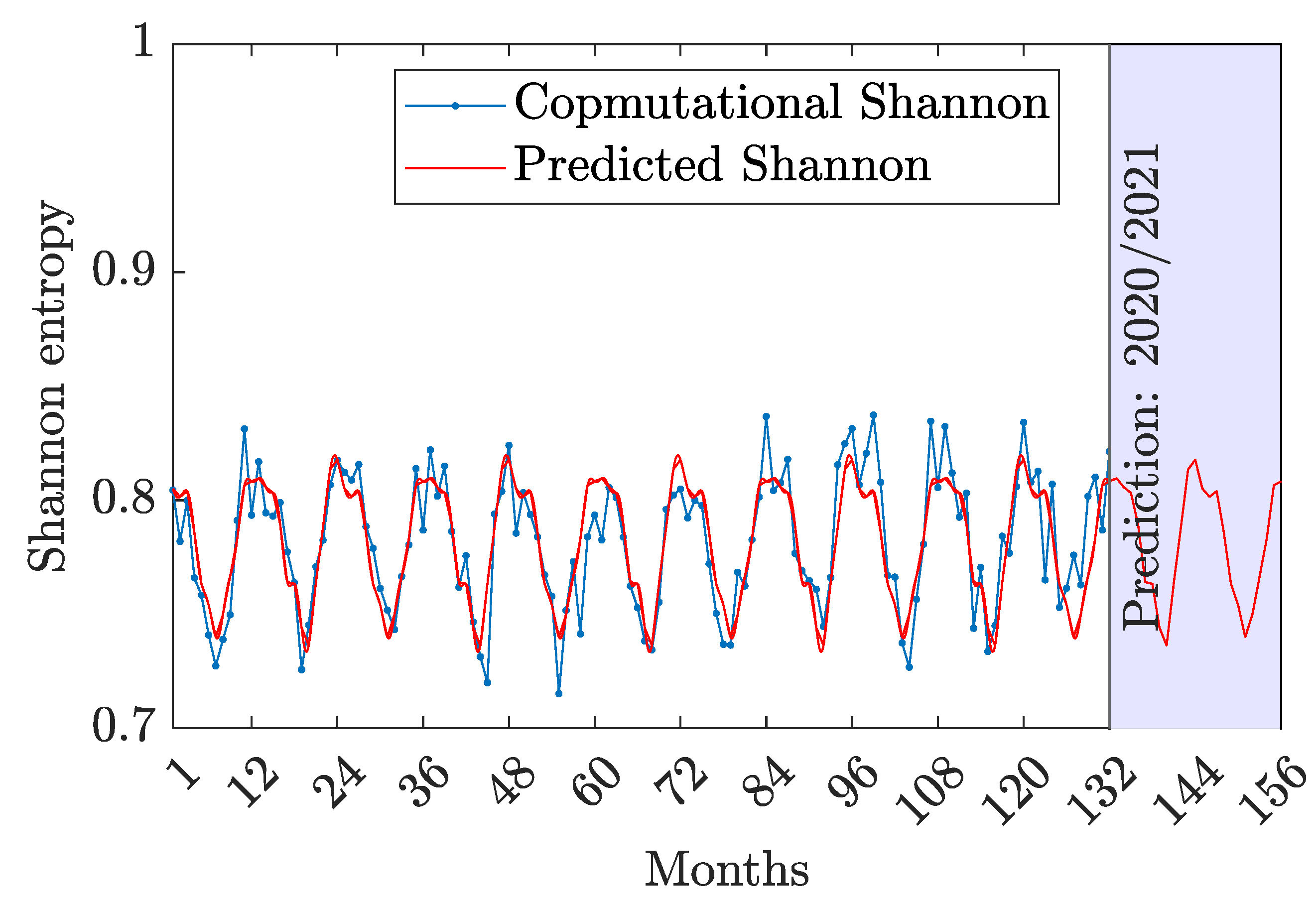
Investigating two distinct types of entropy; $S_H$ and $S_N$ is shown in Figure 7 and Figure 8 respectively. In Figure 7, Shannon entropy is plotted against months by Table 5, Table 7 and Table 8 and Equation (20), in two curves. Clearly, the predicted curve is close to the computational curve with some slight fluctuations after $t>84.$ Shannon entropy describes a noise in the classical information with high values comparing with classical information values.

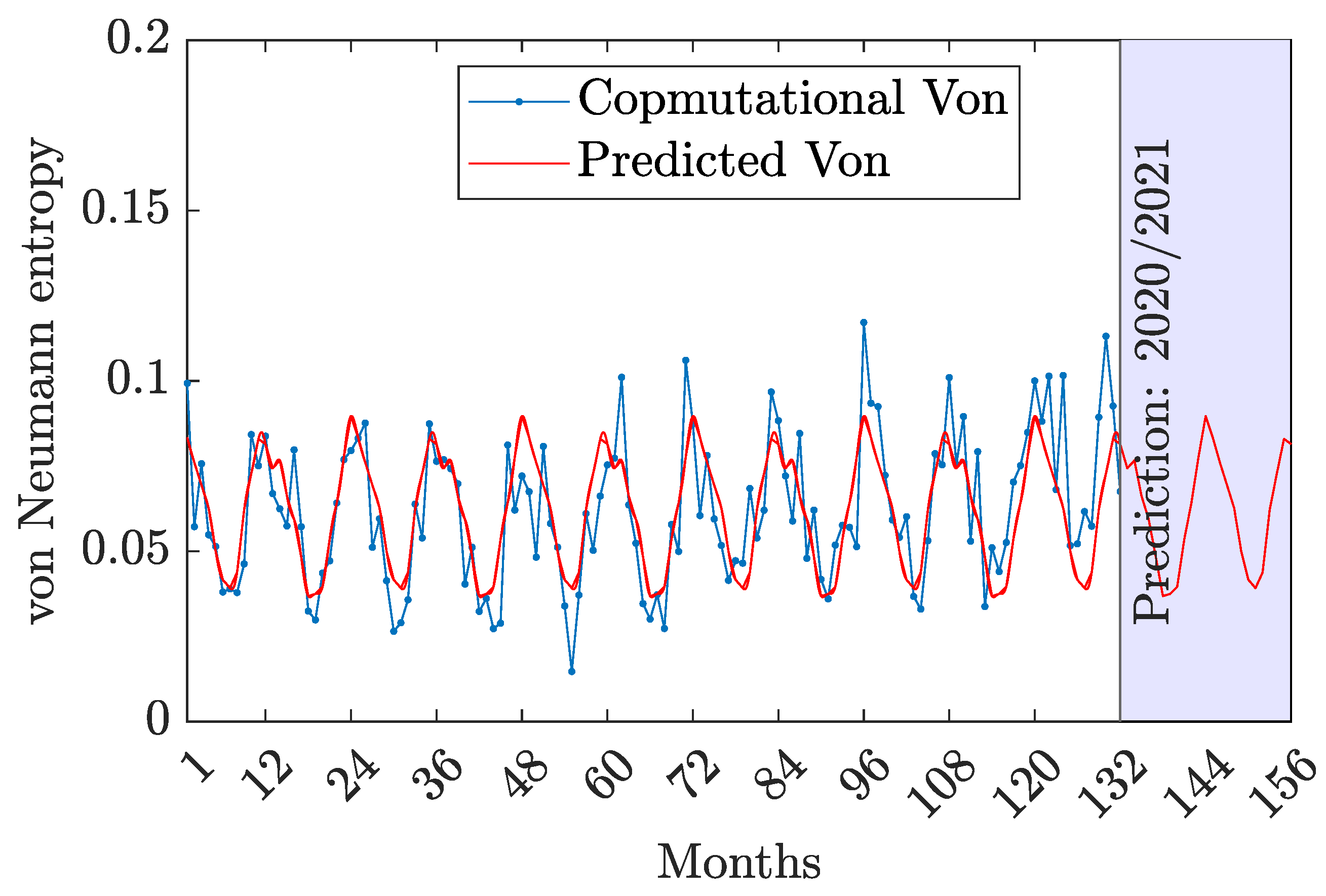
In Figure 8, von Neumann entropy is plotted against months by Table 6, Table 7 and Table 8 and Equation (20), in two curves. von Neumann entropy fluctuates in recent years and has small values which are near to values of the decoherent information. Indeed, the system exhibits a high value of Shannon entropy with respect to the von Neumann entropy approximately 10 times it. There is an oscillatory behavior in both measures due to the periodicity in weather dynamics. Measured values of von Neumann entropy prove the uncertainty of predicting the weather for a month relative to the Shannon entropy.

The analysis of Vancouver’s weather dynamics from 2009 to 2019 through the lens of quantum information theory provides a unique perspective on climate data interpretation. Using concepts from various studies, such as the application of fuzzy logic in decision making [20] and the exploration of quantum entropy in physical systems [21,22], the research integrates advanced mathematical frameworks to model weather patterns. Additionally, insights from quantum classification algorithms [23,24] and the role of entanglement in complex systems [25,26,27,28,29] further enhance the robustness of this analysis. By synthesizing these diverse approaches, the study aims to reveal intricate relationships in weather dynamics, potentially leading to improved predictive models and a deeper understanding of climatic shifts in the Vancouver area.

5. Conclusions

In this paper, we investigated the weather dynamics of Vancouver based on quantum informative measures; the classical and the quantum and the decoherent information, Shannon and von Neumann entropies. We focus on the monthly mixed weather states. The quantum information is in the fornt and is followed by the classical information. The decoherent information occupies in the backyard. Thus, the model is treated in the quantum view since the quantum information is always greatest. Shannon and von Neumann entropies were studied here. It is reasonable that von neumann entropy cannot be neglected as it proves the uncertainity of predicting the weather dynamics for long-term period. We predicted quantum measures dynamics for the next two years and we calculated the errors for them during the compuational period base on a function reduced from Fourier series as function of fitting.

References

1. R. Mendelsohn, J. E. Neumann. The impact of climate change on the United States economy. Cambridge University Press, 2004.
2. J. B. Smith, D. A. Tirpak, The potential effects of global climate change on the United States: Report to Congress, Vol. 1, US Environmental Protection Agency, Office of Policy, Planning, and..., 1989.
3. L. Kalkstein, K. Smoyer, The impact of climate change on human health: some international implications, Experientia 49 (11) (1993) 969–979.
4. K., Charman. False starts and false solutions: current approaches in dealing with climate change. Capitalism Nature Socialism 2008, 19, 29–47. [Google Scholar]
5. Adger, W. Neil; et al. Adaptation to climate change in the developing world. Progress in development studies 2003, 3, 179–195. [Google Scholar] [CrossRef]
6. Smit, Barry, and Olga Pilifosova. Adaptation to climate change in the context of sustainable development and equity. Sustainable Development 2003, 8, 9. [Google Scholar]
7. Pecl, Gretta T.; et al. Biodiversity redistribution under climate change: Impacts on ecosystems and human well-being. Science 2017, 355, eaai9214. [Google Scholar] [CrossRef] [PubMed]
8. Field, Christopher B., and Vicente R. Barros, eds. Climate change 2014–Impacts, adaptation and vulnerability: Regional aspects. Cambridge University Press, 2014.
9. Von Storch, Hans, and Antonio Navarra, eds. Analysis of climate variability: applications of statistical techniques. Springer Science & Business Media, 1999.
10. Von Storch, Hans, and Francis W. Zwiers. Statistical analysis in climate research. Cambridge university press, 2002.
11. Bâra, Adela, Alin Gabriel Văduva. Anomaly Detection in Weather Phenomena: News and Numerical Data-Driven Insights into the Climate Change in Romania’s Historical Regions. International Journal of Computational Intelligence Systems 2024, 17, 134. [Google Scholar] [CrossRef]
12. C. E., Shannon. A mathematical theory of communication. The Bell System Technical Journal 1948, 27, 379–423. [Google Scholar] [CrossRef]
13. Von Neumann, John. Mathematische grundlagen der quantenmechanik. Vol. 38. Springer-Verlag, 2013.
14. M. J., Reinsborough. A ricardian model of climate change in canada. Canadian Journal of Economics/Revue canadienne d économique 2003, 36, 21–40. [Google Scholar]
15. N., Larsson. Adapting to climate change in canada. Building Research & Information 2003, 31, 231–239. [Google Scholar]
16. H. Hengeveld, B. Whitewood, A. Fergusson, An introduction to climate change: A canadian perspective (2005).
17. F. Lenormand, C. R. Duguay, R. Gauthier, Development of a historical ice database for the study of climate change in canada, Hydrological Processes 16 (18) (2002) 3707–3722.
18. Leroyer, S. S. Blair, S. Z. Husain, and J. Mailhot, 2014: Subkilometer Numerical Weather Prediction in an Urban Coastal Area: A Case Study over the Vancouver Metropolitan Area. J. Appl. Meteor. Climatol. 1433; 53. [Google Scholar] [CrossRef]
19. Data link url: https://www.kaggle.com/datasets/luisvivas/weather-north-america?select=vancouver.csv.
20. Hamiden Abd El-Wahed Khalifa, Pavan Kumar, Bayoumi Ali Hassan, An Inexact Rough Interval of Normalized Heptagonal Fuzzy Numbers for Solving Vendor Selection Problem, Appl. Math. Inf. Sci. Volume 15, No. 3 PP: 317-324 (2021). [CrossRef]
21. Serkan Onar, Bayram Ali Ersoy, Kostaq Hila, Krisanthi Naka, (T,S)-Intuitionistic Fuzzy Hyperideals of Γ-Hyperrings, Appl. Math. Inf. Sci. Volume 15, No. 3 PP: 329-342 (2021). [CrossRef]
22. Abdalla, M.S., Obada, A.-S.F., Abdel-Aty, M. Von Neumann entropy and phase distribution of two mode parametric amplifier interacting with a single atom, Annals of Physics, 2005, 318(2), pp. 266–285. [CrossRef]
23. Obada, A.-S.F., Abdel-Aty. Influence of the stark shift and kerr-like medium on the evolution of field entropy and entanglement in two-photon processes. Acta Physica Polonica B 2000, 31, 589–599. [Google Scholar]
24. Abdel-Aty, M., Furuichi, S., Obada, A.-S.F. Entanglement degree of a nonlinear multiphoton Jaynes-Cummings model, Journal of Optics B: Quantum and Semiclassical Optics, 2002, 4(1), pp. 37–43. [CrossRef]
25. Abdel-Aty, A.-H., Kadry, H., Zidan, M., Zanaty, E.A., Abdel-Aty, M. A quantum classification algorithm for classification incomplete patterns based on entanglement measure, Journal of Intelligent and Fuzzy Systems, 2020, 38(3), pp. 2817–2822. [CrossRef]
26. Khalida Inayat Noor, Muhammad Aslam Noor, Hamdy M. Mohamed, Quantum Approach to Starlike Functions, Appl. Math. Inf. Sci. Volume 15, No. 4 (2021) PP: 437-441. [CrossRef]
27. Amer Basim Shaalan, Nadir Fadhil Habubi, Sami Salman Chiad, Ziad Abdulahad Toma, New Design of Hairpin-Koch Fractal Filter for Suppression of Spurious Band, Int. J. Thin Film Sci. Tech. Vol. 2 No. 3 (2013) PP: 217-221.
28. Alaa Zuhir Al Rawashdeh, Asma Rebhi Al Arab, Noura Nasser Alqahtani and Zineb Hadmer, The Sociological Understanding, for Corona Crises and its Reflections on Society: An Inductive Analytical Vision, J. Stat. Appl. Prob. Vol. 10, No. 1 (Mar. 2021), PP:267-286. [CrossRef]
29. Yeqian Liu, Extended Bayesian Framework for Multicategory Support Vector Machine, J. Stat. Appl. Prob. 9 (2020) 1-11. [CrossRef]
Figure 1. Vancouver weather variables; maximum temperature, minimum temperature, and dew point. (a) Maximum temperature; (b) Minimum temperature; (c) Dew point.
Preprints 149843 g001
Figure 2. Vancouver weather variables; cloud cover, humidity, and precipitation.
Preprints 149843 g002
Figure 3. Vancouver weather variables; total snow, pressure, and wind speed.
Preprints 149843 g003
Figure 4. Computational and predicted classical information.
Preprints 149843 g004
Figure 5. Computational and predicted quantum information.
Preprints 149843 g005
Figure 6. Computational and predicted decoherence information.
Preprints 149843 g006
Figure 7. Computational and predicted Shannon entropy.
Preprints 149843 g007
Figure 8. Computational and predicted Shannon entropy.
Preprints 149843 g008