
Submitted:
19 February 2025
Posted:
19 February 2025
You are already at the latest version
Abstract
Machining process optimization involves selecting appropriate control variable (CV) settings to achieve desired evaluation variable (EV) outcomes. With the emergence of Open Data (OD) in smart manufacturing, machining optimization can now incorporate diverse CV-EV-centric data beyond local ones. This study investigates whether CV-EV-centric OD provides sufficient information, whether its analysis can yield actionable insights, and how suitable optimization methods are for OD-driven analysis. To explore this, Analysis of Variance (ANOVA) and Signal-to-Noise Ratio (SNR) were applied as conventional methods, while Possibility Distribution (PD) was used as a non-conventional method. The results indicate that PD offers an integrated solution, combining the strengths of ANOVA and SNR, for extracting actionable insights from the OD. It (PD) also enhances interpretability for some CV-EV-relationships and enables the formation of linguistic rules—an aspect not directly achievable through ANOVA or SNR alone. The findings suggest that combining conventional and non-conventional methods improve the analysis of OD-driven machining data, contributing to more structured optimization frameworks in smart manufacturing.
Keywords:
Machining
; Optimization
; Open Data
; ANOVA
; SNR
; Possibility Distribution
; Fuzzy Number
; Uncertainty
; Interpretability
1. Introduction
Manufacturing processes transform raw materials into finished products and are broadly categorized into three types: (1) additive manufacturing (material is added layer by layer to create a shape), (2) subtractive manufacturing (material is removed to create a shape), and (3) formative manufacturing (material is reshaped without material addition or removal) [1,2,3,4]. Among these, subtractive manufacturing—commonly known as machining—remains fundamental to industrial production, enabling precise material removal to achieve desired geometries and surface qualities. This study specifically focuses on machining processes, and hereafter, the term manufacturing process will refer to machining operations.
As seen in Figure 1, in a machining process, a cutting tool removes material from a workpiece. This operation is governed by process parameters such as cutting speed (vc), feed rate (f), radial/axial depth of cut (ap/ae), and spindle speed (N). These parameters, which directly influence the machining, are commonly referred to as Control Variables (CVs) [2,5]. As such, CVs define the input conditions of a machining process, and their selection significantly impacts machining performance. As machining progresses, the interaction between the tool and the workpiece gives rise to various phenomena, such as chip formation, tool wear, heat generation, and cutting force. These phenomena, in turn, affect measurable performance indicators, such as surface roughness, cutting force, material removal rate (MRR), and tool wear. These indicators are referred to as Evaluation Variables (EVs) since they quantify machining performance [2,5]. As seen in Figure 1, the relationship between CVs and EVs is not always straightforward. For instance, an increase in f generally leads to an increase in both surface roughness and MRR. While a higher MRR is desirable for improved productivity, increased roughness negatively impacts surface quality. This behavior highlights fundamental problem of machining optimization: how should f be selected to achieve a balance between maximizing MRR and minimizing surface roughness? Section 2 presents a literature review on machining optimization and relevant methods.
From the viewpoint of smart manufacturing [6,7,8], machining optimization can be approached through the integration of Open Data (OD)—publicly available machining datasets contributed by multiple sources, including research institutions, industries, and digital manufacturing platforms. Instead of relying solely on locally acquired CV-EV-centric data, OD enables a broader, data-driven perspective where insights can be derived from diverse machining setups, tools, and conditions. Figure 2 shows an OD lifecycle that can be followed for enabling OD-driven optimization.
As seen in Figure 2, the upstream of the lifecycle creates OD (also described in [6]). This includes the documentation of CV-EV-centric data, wrangling the data into a structured machine-readable format such as JSON, and storing the machine-readable data in a cloud-based repository to ensure accessibility. Through this process, OD becomes part of a larger interconnected ecosystem, often referred to as the Digital Manufacturing Commons (DMC) [7,9]—a shared infrastructure where manufacturing data (process-relevant data, CAD models, systems, algorithms, and alike) is openly available for analysis and application across different workspaces. As seen in Figure 2, the downstream of the lifecycle focuses on utilizing the created OD. This involves acquiring OD, analyzing it to extract relevant insights, and adapting the extracted knowledge for specific machining optimization tasks as needed. At this stage, analyzing OD raises key research questions, such as whether CV-EV-centric OD provides sufficient information to determine optimal CV settings, whether its analysis can yield actionable knowledge, and to what extent existing methods are suitable for OD analysis. This study investigates these questions by employing three methods: two conventional approaches, Analysis of Variance (ANOVA) [10,11,12,13] and Signal-to-Noise Ratio (SNR) [13,14,15,16], and a non-conventional approach, Possibility Distribution (PD) [17,18], to analyze CV-EV-centric OD for a machining process called turning.
For better understanding, the rest of this article is organized as follows. Section 2 provides a literature review on machining optimization. Section 3 describes the abovementioned methods. Section 4 presents the OD and analyses results. Section 5 discusses the obtained results. Section 6 provides the concluding remarks of this study.
2. Literature Review
This section presents a literature review on the machining process optimization. For this, a bibliographic dataset from Scopus®, a well-known bibliographic database, is acquired, analyzed, and studied. The dataset is acquired using the following search criteria. Keyword: machining process optimization; Subject area: Engineering; Document type: Article; Source type: Journal, Publication stage: Final, and Year: 2000-2025. Data related to 7,361 (seven thousand three hundred sixty-one) journal articles are collected. Section 2.1 presents an overview of the abovementioned data. Section 2.2 presents some selected works, describing how different methods are being applied for the sake of optimization.
2.1. Overview
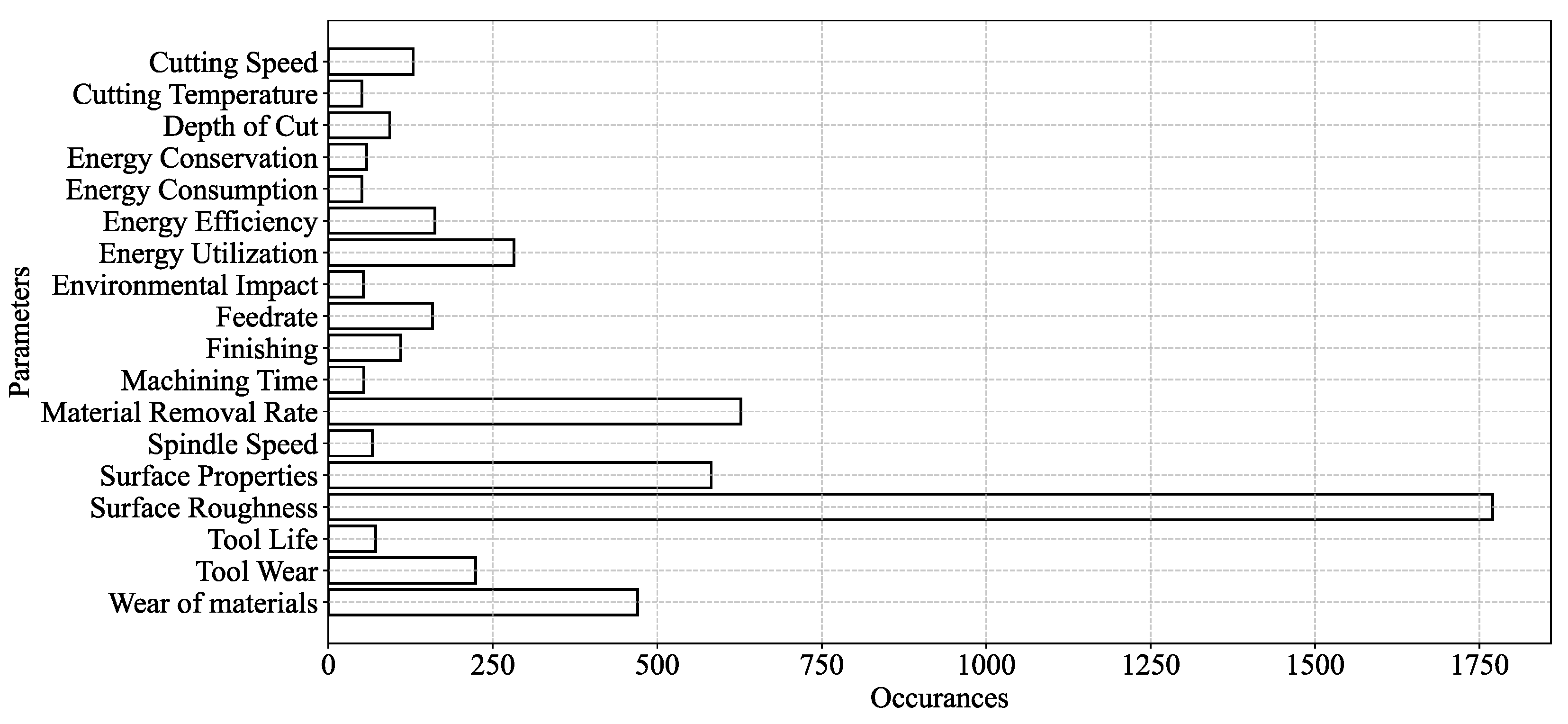
The abovementioned bibliographic dataset is analyzed to understand: (1) which data analyses methods are being used frequently for optimization, (2) which processes are being considered frequently for optimization, and (3) which CV-EVs are being considered frequently for optimization. For this, the number of occurrences of the relevant keywords (here, ‘Index Keywords’) are evaluated. Figure A2, Figure A3 and Figure A4 (see Appendix A) show some of the results, respectively. Figure A2 shows that the frequently used methods include analysis of variance, genetic algorithms, neural networks, grey relational analysis, regression analysis, particle swarm optimization, signal to noise ratio, principal component analysis, and fuzzy inference. Figure A3 shows that frequently considered processes include grinding, milling, cutting, electrical discharge machining, and turning. Figure A4 shows that frequently considered CV-EVs include surface roughness, surface properties, tool wear, wear of materials, material removal rate, energy utilization, energy efficiency, cutting speed, feed rate, spindle speed, depth of cut, and machining time.
Though the above keyword-based analysis provides a comprehensive outlook on the methods, processes, and CV-EVs, the role of different methods in process optimization is yet to understand. Are the methods used to perform the same task while optimizing? Or, do the methods have different roles? How do they complement each other in optimization tasks? Keeping this in mind, the acquired articles are further studied, as follows.
Machining process optimization typically begins with a Design of Experiments (DoE) approach, where CVs are systematically varied using structured experimental designs like Taguchi’s orthogonal arrays [10,19,20,21,22], Full Factorial Designs [23,24], and Response Surface Methodology (RSM) [11,14]. Based on the DoE, experiments are conducted and EV data are collected. This creates a CV-EV-centric data matrix. The CV-EV-centric data are then analyzed using statistical methods to determine the effects of CVs on the EVs. These methods include Analysis of Variance (ANOVA) for identifying significant CVs [10,11,12,13,25,26,27], Signal-to-Noise Ratio (SNR) for evaluating variability and identifying optimal CV states [13,14,15,16,28], and Regression Models for developing predictive CV-EV relationships [20,28]. In some cases, techniques like Principal Component Analysis (PCA) and clustering methods like Support Vector Machine (SVM) are also used to interpret complex datasets [29,30,31,32,33,34]. Additionally, Grey Relational Analysis (GRA) is often applied when multiple EVs need to be evaluated together. GRA converts multiple EVs into a single ranking index, helping to determine the optimal CVs for the experimental run without requiring complex computations [33,35,36,37].
Beyond the abovementioned statistical methods, machine learning models like Artificial Neural Networks (ANN) and Support Vector Regression (SVR) are also used to learn patterns directly from CV-EV-centric data [10,19,25,38,39,40]. When the CV-EV space is large and involves multiple local optima, metaheuristic algorithms such as Genetic Algorithms (GA), Particle Swarm Optimization (PSO), and Simulated Annealing (SA) are used to iteratively explore the optimal conditions [19,25,37,38,41,42]. In the case of evaluating multiple EVs together, multi-objective optimization methods like NSGA-II and MO-GA are used [37,43,44]. They generate a pareto front, providing a set of optimal trade-offs rather than a single solution. For the sake of real-time adaptation, where EVs such as tool wear, material hardness, and cutting forces change dynamically, machine learning models such as Reinforcement Learning (RL) is employed [41,42]. It (RL) learns from sensor feedback and past outcomes, and update the CVs dynamically.
Now, returning to DoE, while it provides a structured way to explore CV-EV relationships through planned experimentation, Bayesian Optimization (BO) offers a flexible, data-driven alternative [19,45,46]. Unlike DoE, BO does not require a predefined CV matrix but instead adapts test conditions iteratively based on prior results. If a historic CV-EV dataset is available, BO leverages this data to identify CV settings, reducing the need for additional experiments. If no prior data exists, BO begins with a few initial exploratory trials and then refines subsequent test conditions based on the observed outcomes. This approach is particularly useful when experimentation is costly or when the search space is large, making BO a complementary strategy to DoE.
Additionally, to handle uncertainty inherent to machining decisions, methods such as Fuzzy Inference [5,47,48,49] and Possibility Distribution (PD) [17,18] are used for facilitating expert-driven reasoning. These methods use fuzzy membership functions to handle imprecise CV-EV relationships, generating linguistic rules for the sake of optimization.
2.2. Selected Studies
As discussed in Section 2.1, machining process optimization involves a diverse set of methods, each addressing different challenges. Statistical approaches such as ANOVA, SNR, and regression models help quantify the influence of CVs on EVs, while machine learning techniques like ANN, SVR, and RL enable predictive modeling and real-time adaptation. Metaheuristic algorithms such as GA, PSO, and NSGA-II explore large search spaces, and fuzzy-based approaches provide decision-making flexibility in uncertain conditions. While these methods serve distinct roles in machining process optimization, their practical applications vary across studies. To examine how they are implemented, the following section reviews some selected works.
Agarwal et al. [13] studied CNC turning of 16MnCr5 steel using TiN-coated TNMG160404 carbide inserts, to determine the optimal CVs (cutting speed, feed rate, and depth of cut) for maximizing the EV (material removal rate) and minimizing the EV (surface roughness). Experiments were conducted based on Taguchi L9 DoE. ANOVA and SNR were applied to analyze the influence of CVs on the EVs, and optimal CV states, respectively.
Perumal et al. [11] studied CNC turning of AA359 alloy using titanium carbonitride–coated CBN inserts, to determine the optimal CVs (spindle speed, feed rate, and depth of cut) for maximizing the EV (material removal rate) and minimizing the EV (surface roughness). Experiments were conducted based on Taguchi L16 DoE. ANOVA was applied to analyze the influence of CVs, while the General Linear Model (GLM) and Response Surface Methodology (RSM) were used to determine their optimal states.
Gangwar et al. [28] studied dry turning of EN31 steel using CNMA 120208 tungsten carbide inserts to determine the optimal CVs (cutting speed, feed rate, and depth of cut) for maximizing the EV (material removal rate) and minimizing the EV (surface roughness). Experiments were conducted based on Taguchi L18 DoE. SNR analysis was used to assess the impact of CVs on the EVs, while ANOVA developed regression equations describing their relationship. These equations were then used as the objective function in Grasshopper Optimization Algorithm (GOA) to determine the optimal CVs.
Saleem and Mehmood [50] studied turning of Inconel 718 using TiAlN PVD-coated SNMG 120408 NN LT 10 inserts, to determine the optimal CVs (cutting speed, feed rate, and air pressure) for minimizing the EVs (tool wear and surface roughness). Experiments were conducted based on Taguchi L9 DoE. ANOVA was applied to analyze the influence of CVs on the EVs, and mean value calculations were used to determine optimal CV states.
Chanie et al. [38] studied wire cut EDM of mild steel AISI 1020 using a DK7732C machine to determine the optimal CVs (peak current, pulse on/off time, and wire feed rate) for maximizing the EV (material removal rate) and minimizing the EV (surface roughness). Experiments were conducted based on Taguchi L9 DoE. An Artificial Neural Network (ANN) model was developed and integrated with a multi-objective Genetic Algorithm (GA) for optimization of CVs.
Teimouri et al. [12] studied rotary turning with ultrasonic vibration of aluminum 7075 aerospace alloy using tungsten carbide RCMT10T3 MO Lamina Co inserts, to determine the optimal CVs (cutting velocity, tool rotary speed, and feed rate) for minimizing the EVs (cutting force and surface roughness). Experiments were conducted based on Taguchi L9 DoE. ANOVA was applied to analyze the influence of CVs on EVs, and the Desirability Function Approach (DFA) was used to determine the optimal CVs levels.
Banerjee and Maity [15] studied turning of Nitronic-50 using MT-PVD inserts, to determine the optimal CVs (cutting velocity, feed, and depth of cut) for minimizing the EV (tool wear) and surface roughness while maximizing the EV (material removal rate). Twenty experiments were conducted, resulting in CV-EV-centric data. ANOVA was applied to analyze the influence of CVs on EVs. The Multi-Objective Optimization by Ratio Analysis (MOORA), Teaching-Learning-Based Optimization (TLBO), and SNR techniques were used to determine the optimal CV levels.
Sun et al. [51] studied milling of TC4 (Ti-6Al-4V) using flat-end and ball-end cutters, to determine the optimal CVs (spindle speed, feed, and axial/radial depth of cut) for maximizing cutting efficiency while minimizing the EVs (surface roughness and cutting force). The Technique for Order Preference by Similarity to an Ideal Solution (TOPSIS) was first applied to identify significant CV levels. A combined TOPSIS and Adversarial Interpretive Structural Modeling (TOPSIS-AISM) method was then used for optimization. Finally, the results of traditional TOPSIS and TOPSIS-AISM were compared.
Wang et al. [36] studied grinding of AISI 1045 steel using a WA60L6 V grinding wheel, to determine the optimal CVs (feed velocity, depth of cut, and cooling/lubrication conditions) for minimizing the EVs (residual stress, surface roughness, production cost, and CO₂ emission) while maximizing the EVs (production rate and operator health). Experiments were conducted based on Taguchi L9 DoE. Grey Relational Analysis (GRA) was applied to analyze the influence of CVs on EVs and determine their optimal levels.
Karthick et al. [26] studied milling of Inconel 718 using ACK 300 Sumitomo carbide-coated ball nose milling inserts, to determine the optimal CVs (traverse speed, torch height, arc current, and gas pressure) for minimizing the EVs (kerf deviation and surface roughness) while maximizing the EV (micro hardness). Experiments were conducted based on DoE. ANOVA was applied to analyze the influence of CVs on EVs, followed by Moth-Flame Optimization (MFO) to determine optimal CV levels. The results from ANOVA and MFO were then compared.
Boga and Koroglu [25] studied milling of high-strength carbon fiber composite plates under dry conditions using TiAlN-coated and Mikrograin Carbide-C10 tools, to determine the optimal CVs (cutting tool, feed rate, and spindle speed) for minimizing the EV (surface roughness). Experiments were conducted using Taguchi mixed orthogonal array L32 (21 × 42). ANOVA was applied to analyze the influence of CVs on EVs, identifying cutting tool and feed rate as the most significant factors. The optimal CV combination was found to be a TiAlN-coated tool, 5000 rpm spindle speed, and 250 mm/rev feed rate. A feed-forward backpropagation neural network (NN) was also developed to estimate EV values, with a genetic algorithm (GA) assisting in parameter selection.
Kechagias [16] studied end milling of aluminum alloy 5083 using a carbide tool, to determine the optimal CVs (feed rate, cutting speed, and depth of cut) for minimizing the EV (surface roughness). Experiments were conducted based on Taguchi L27 DoE. Analysis of Means (ANOM) was applied to identify significant CVs affecting EVs, while SNR analysis was used to determine their optimal levels.
Mohanta et al. [37] studied CNC turning of Al 7075 using CVD-coated carbide inserts, to determine the optimal CVs for minimizing the EVs (surface roughness and cutting force). Grey Relational Analysis (GRA) and Desirability Function Analysis (DFA) were first applied to optimize CVs. Multi-Objective Genetic Algorithm (MOGA) and Multi-Objective Particle Swarm Optimization (MOPSO) were then used for further optimization.
Kosarac et al. [10] studied milling of titanium alloy Ti-6Al-4V using a spindle milling cutter (HF 16E2R030A16-SBN10-C), to determine the optimal CVs (cutting speed, feed rate, depth of cut, and cooling/lubricating method) for minimizing the EV (surface roughness). Experiments were conducted based on Taguchi L27 DoE. ANOVA was applied to analyze the influence of CVs on EVs, identifying feed rate as the most significant factor. SNR analysis was used to determine the optimal CV levels. Additionally, neural networks and Random Forest were used to develop a predictive model for surface roughness based on the collected dataset, with Random Forest performing better on small datasets.
Tanvir et al. [35] studied turning of AISI 304 stainless steel using high-speed steel single point cutting tool, to determine the optimal CVs (cutting speed, feed rate, and depth of cut) for maximizing the EV (material removal rate) while minimizing the EVs (surface roughness, cutting force, power consumption, heat rate, and peak tool temperature). Simulations and experiments were conducted to obtain EV values across different machining settings. A hybrid multi-objective optimization approach integrating Grey Relational Analysis (GRA) with the Whale Optimization Algorithm (WOA) was then applied to determine the optimal CV levels.
Mongan et al. [19] studied CNC end milling of aluminum 6061 using a 4-flute solid carbide square end mill with a titanium nitride coating, to determine the optimal CVs (feed per tooth, cutting speed, and depth of cut) for maximizing the EV (material removal rate) while minimizing the EV (surface roughness). A full factorial parametric study was conducted, and ANOVA was applied to analyze the influence of CVs on EVs. An Ensemble Neural Network (ENN) was then developed using Genetic Algorithm-optimized Artificial Neural Network (GA-ANN) base models, with hyperparameters tuned via Bayesian optimization. The trained ENN was used to identify optimal CV combinations for achieving a predefined surface roughness while maximizing material removal rate.
Chowdhury et al. [18] studied rotary ultrasonic machining of Ti6Al4V alloys, to analyze the effects of CVs (ultrasonic power, feed rate, spindle speed, and tool diameter) on EVs (cutting force, tool wear, overcut error, and cylindricity error). Experiments were conducted following a Taguchi L36 DoE approach, and the effects of CVs were evaluated using possibility distributions constructed from the experimental data. These distributions, represented as trapezoidal fuzzy numbers, were used to quantify uncertainty and identify optimal CVs.
Bouhali et al. [20] studied dry turning of 2017A aluminum alloy using a carbide-cutting tool, to determine the optimal CVs (cutting speed, feed rate, and depth of cut) for minimizing the EVs (surface roughness and cutting temperature). Experiments were conducted using the Taguchi L16 DoE approach with three factors and four levels. The signal-to-noise (S/N) ratio and ANOVA were applied to analyze the influence of CVs on EVs, identifying depth of cut as the most significant factor. Regression analysis was then used to develop mathematical models for predicting surface roughness and cutting temperature and for determining optimal cutting conditions.
Ullah and Harib [5,49] argued that optimizing machining processes using CV-EV-centric data requires transparency rather than relying solely on black-box models. They demonstrated this using the ID3-based decision tree, which effectively extracts patterns but inherently excludes certain CVs, leaving their relationship with the EV unknown. This lack of interpretability creates operational challenges, as crucial factors may remain hidden. To address this, they proposed a human-assisted knowledge extraction system integrating probabilistic and fuzzy reasoning, ensuring user involvement. This underscores a broader concern with black-box methods, which optimize outcomes without revealing decision processes, making insights difficult to apply [7,52,53,54,55]. Unlike statistical approaches that allow direct human reasoning, many ML models operate independently after data input, limiting user engagement. Maintaining transparency and involving users in knowledge extraction ensures that optimization remains interpretable and actionable.
In sum, the literature review highlights various methods used in machining optimization, including statistical techniques, machine learning, metaheuristic algorithms, and fuzzy inference and uncertainty quantification tools. However, these methods are typically applied in controlled environments with structured DoE frameworks. As introduced in Section 1, OD lacks such predefined structures and integrates data from multiple sources, making it unclear how well existing methods perform in OD-driven analysis. To address this, this study selects ANOVA, SNR, and PD among others. These methods are more humanly comprehensible than black-box approaches and computationally accessible, making them practical for OD, which is intended for broad usability, including small and medium-sized enterprises (SMEs). Unlike complex machine learning models, ANOVA, SNR, and PD can be applied with basic tools like spreadsheets, ensuring feasibility in OD-driven analysis. The following section describes these methods.
3. Methods
This section describes the methodological framework and mathematical formulations underlying three data analysis methods: (1) Analysis of Variance (ANOVA), (2) Signal-to-Noise Ratio (SNR), and (3) Possibility Distribution (PD), as outlined in Subsections 3.1, 3.2, and 3.3, respectively.
3.1. Analysis of Variance (ANOVA)
Analysis of Variance (ANOVA) is a generic name for a set of statistical methods to know whether two or more groups of datasets are statistically different [56,57]. The most commonly used types of ANOVA include: (1) Single-Factor (One-Way), (2) Two-Factor with Replication, and (3) Two-Factor without Replication [56,58,59]. Using ANOVA, it is possible to know whether an independent variable significantly affects a given dependent variable. For this reason, these three types of ANOVA have been extensively used in manufacturing process optimization. For a better understanding, the abovementioned ANOVA-types are described below.
‘Single-Factor ANOVA’ tests whether a given independent variable significantly affects a given dependent variable. For example, consider one independent variable called cutting speed and one dependent variable called tool wear. Single-Factor ANOVA then tests whether the cutting speed significantly affects the tool wear. In this case, Single-Factor ANOVA may consider the datasets of cutting speed for (say) three states, 200 m/min, 300 m/min, and 400 m/min, and the corresponding tool wear. As far as ‘Two-Factor ANOVA with Replication’ is concerned, it tests whether two given independent variables significantly affect a given dependent variable. For example, consider two independent variables called cutting speed and material removal rate, and one dependent variable called tool wear. Two-Factor ANOVA with Replication then tests whether the cutting speed and the material removal rate collectively affect the tool wear and to what extent. In this case, Two-Factor ANOVA with Replication considers the datasets of cutting speed for (say) three states, 200 m/min, 300 m/min, and 400 m/min, and three states of material removal rate, 10 cm³/min, 15 cm³/min, and 20 cm³/min, and the corresponding tool wear. As far as ‘Two-Factor ANOVA without Replication’ is concerned, it tests whether two given independent variables significantly affect a dependent variable when there is only one observation for each combination of variable states. For example, consider two independent variables called cutting speed and material removal rate, and one dependent variable called tool wear. This Two-Factor ANOVA without Replication evaluates whether cutting speed, material removal rate, and their interaction significantly affect tool wear. In this case, Two-factor ANOVA without Replication considers cutting speed datasets for (say) three states, 200 m/min, 300 m/min, and 400 m/min, and three states of material removal rate, 10 cm³/min, 15 cm³/min, and 20 cm³/min with a single measurement taken for each combination.
Among the three ANOVA types mentioned above, Single-Factor (One-Way) ANOVA is the most commonly used in manufacturing process optimization [58,59]. Therefore, in this study, ANOVA refers specifically to Single-Factor (One-Way) ANOVA, which is also employed in this study for data analysis (see Section 4). Accordingly, the following discussion outlines its methodological framework and mathematical formulation to provide a comprehensive understanding.
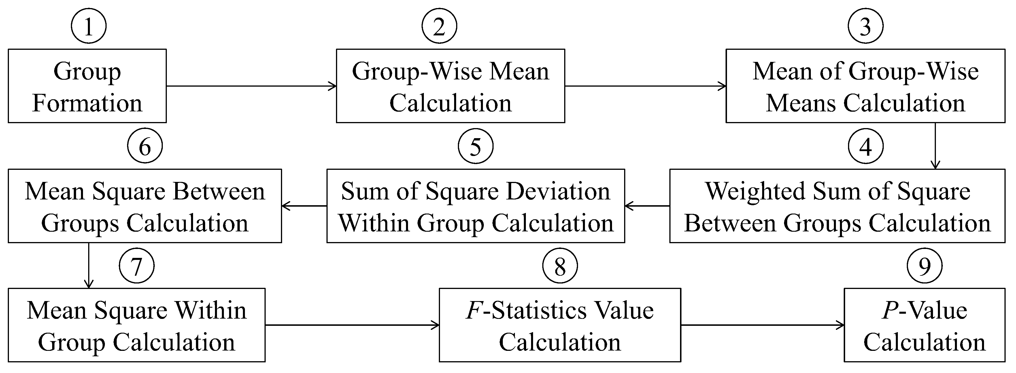
Figure 3 schematically illustrates the methodological framework underlying the Single-Factor ANOVA. As seen in Fig. 3, the Single-Factor ANOVA method consists of nine (9) calculation steps. The goal of these calculations is to determine the value of a probability denoted as P. An independent variable significantly affects a given dependent variable when P is less than a given level of significance (e.g., α = 0.05) [58,60,61,62,63]. The step-by-step formulation of how to calculate P is presented below.
Figure 3.
Outlining Single-Factor (One-Way) ANOVA method.
Let G be the set of groups of datasets, i.e., G = {Gj | j = 1,…,m} where Gj denotes the j-th group (also denoted as state). Each group consists of some numerical data denoted as Gj = {gij ∈ ° | i = 1,…,nj}. The group mean (strictly speaking, group average) denoted as MGj is calculated as follows:
𝑀𝐺𝑗 = 1𝑛𝑗𝑖=1𝑛𝑗𝑔𝑖𝑗
The overall mean denoted as OM is calculated as follows:
𝑂𝑀= 1𝑚𝑗=1𝑚𝑀𝐺𝑗
The weighted sum of squares between groups denoted as SSB is calculated as follows:
The sum of square deviations within group denoted as SSW is calculated as follows:
The mean square between groups denoted as MSB is calculated as follows:
The mean square within groups denoted as MSW is calculated as follows:
The F-statistics value denoted as F is calculated as follows:
The P-value denoted as P is calculated as follows:
In Equation (8) B represents the beta function, represents the degrees of freedom between groups, and represents the degrees of freedom within groups. and are calculated as follows.
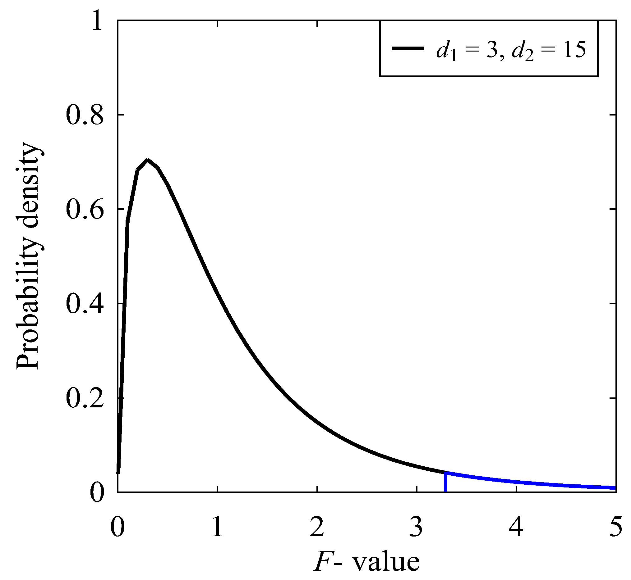
Figure 4 shows F-distribution curve with F-critical value. In Figure 4, the x-axis represents F-value and the y-axis represents probability density. Considering d1 = 3, d2 = 15, and α = 0.05, F-critical value is 3.28, as shown in Figure 4. If F-value is larger than this F-critical value, then it implies that the corresponding independent variable significantly affects the dependent variable [60,61,62].
Figure 4.
F-distribution curve with F-critical value.
3.2. Signal-to-Noise Ratio (SNR)
Taguchi method is developed by a Japanese scientist named Dr. Genichi Taguchi during the 1950s and 1960s [64]. Different fields of engineering use this method to optimize manufacturing processes and systems. The Taguchi method utilizes a set of orthogonal arrays to make relationship between independent variables and dependent variables with as few experiments as possible [10,19,20]. Orthogonal arrays consider states in independent variable(s) to ensure all states independently tested with minimal experimental runs. For example, the Taguchi method considers one independent variable called cutting speed for (say) three states, 200 m/min, 300 m/min, and 400 m/min. Then, the Taguchi method uses a statistical measure of performance called Signal-to-Noise Ratio (SNR) to identify the optimal state of independent variable(s). The SNR is the ratio of signal and noise. The term ‘Signal’ represents mean, and the ‘Noise’ represents standard deviation from mean. The SNR finds the optimal state of independent variables converting experimental result of dependent variables into a value. The largest value of SNR means the optimal state of independent variables [10,15,16,65,66]. There are three types of SNR used for analysis, namely the Smaller-the-Better, the Optimal-the-Better, and the Larger-the-Better. For the sake of better understanding, these three types of SNR are described in Subsections 3.2.1-3.2.3, respectively.
3.2.1. Smaller-the-Better (STB)
Smaller-the-Better (STB)-SNR finds the optimal state of a given independent variable for minimizing given a dependent variable. For example, consider one independent variable called cutting speed and one dependent variable tool wear. In this case, STB-SNR may consider the datasets of cutting speed for (say) three states, 200 m/min, 300 m/min, and 400 m/min, and the corresponding tool wear. STB-SNR then finds the optimal state of cutting speed for minimizing tool wear. For each state, the STB-SNR denoted as is calculated as follows.
In Equation (11), represents the Smaller-the-Better S/N ratio of j-th group (also denoted as state). . represents the individual numerical data of j-th group of the dependent variable and represents the total amount of data of the group. The largest value of indicates the optimal state of independent variable for minimizing the dependent variable.
3.2.2. Larger-the-Better (LTB)
Larger-the-Better (LTB)-SNR finds the optimal state of a given independent variable for maximizing a given dependent variable. For example, consider one independent variable cutting speed and one dependent variable material removal rate. In this case, LTB-SNR may consider the datasets of cutting speed for (say) three states, 200 m/min, 300 m/min, and 400 m/min, and the corresponding material removal rate. LTB-SNR then finds the optimal state of cutting speed for maximizing material removal rate. For each state, the LTB-SNR denoted as is calculated as follows.
The largest value of indicates the optimal state of independent variable for maximizing the dependent variable.
3.2.3. Nominal-the-Better (NTB)
Nominal-the-Better (NTB)-SNR finds the optimal state of a given independent variables to obtain a target value of a given dependent variable. For example, consider one independent variable called cutting speed and one dependent variable called surface roughness. In this case, NTB-SNR may consider the datasets of cutting speed for (say) three states, 200 m/min, 300 m/min, and 400 m/min, and the corresponding surface roughness. NTB-SNR then finds the optimal state of cutting speed to obtain value of surface roughness. For each state, the NTB-SNR denoted as is calculated as follows:
In Equation (13), t presents the target value of dependent variable. The largest value of indicates the optimal state of independent variable to obtain the target value of dependent variable.
3.3. Possibility Distribution (PD)
A possibility distribution is a probability-neutral representation of uncertainty in a dataset, often associated with fuzzy set theory [67,68,69,70]. It is used when precise probabilistic data is unavailable, providing a structured way to express the plausibility of different values, particularly in cases of scarce, incomplete, or difficult-to-quantify data. In fuzzy systems, it represents degrees of possibility rather than strict probabilities, making it applicable to engineering, materials science, environmental modeling, and decision-making under epistemic uncertainty. Studies have used it to analyze material properties [71,72], surface roughness models and surface of bi-metal components [73,74], CO₂ emissions [75], sensor signal-based digital twins [76], and machining process optimization [17,18]. Nevertheless, the mathematical formulations for inducing the possibility distribution from a given set of numerical data are described below.
Let be n data points, as shown in Figure 5.
Let , , be a point-cloud in the universe of discourse so that and . Let and two square boundaries so that the vectors of the vertices of and (in the anti-clockwise direction) are ((), (), (), ()) and ((), (), (), ()), respectively, . As such, is their common vertex of and . For example, consider the arbitrary point-cloud shown in Figure 6. As seen in Figure 6, the universe of discourse G = [0 0.45]. Notice the relative positions of boxes denoted by and in Figure 6. The boxes are connected their common vertices.
Let () and be two subjective probabilities, wherein () and () represent the degrees of chances that the points in the point-cloud are, in and , respectively. As such, these functions are defined by the following mappings:
The typical nature of the functions defined in Equations (14) and (15) are illustrated in Figure 7 using the information of the point -cloud shown in Figure 6. Note that ( increases with the increase in g and the opposite is true for (). It is worth mentioning that (( = 1 (see Figure 8). This means that (( does not serve the role of ‘cumulative probability distribution’. A cumulative probability distribution can however be formulated by using the information of ( and (, as shown in Figure 7.
Considered a mapping that maps g into the minimum of ( and ( as follows:
In Equation (16), , if the point-cloud is a point; otherwise, . Figure 8 shows the nature of for ( and (). The area under is given by:
There is no grantee that . Otherwise, could have been considered a probability distribution of the underlying point-cloud. However, a function can defined, as follows:
can be considered a cumulative probability distribution because max for , , Figure 9 shows the natures of derived from shown in Figure 8. The cumulative probability distribution defined in Equation (18) produces a probability distribution (g). Thus, the following formulation holds:
Figure 10 shows the probability distribution underlying shown in Figure 9. It is needless to say that the area under the probability distribution is a unit and remains in the bound of [0, 1].
From the induced probability distribution , a possibility distribution given by the membership function can be defined based on the heuristic rule of probability-possibility distribution transformation-that the degree of possibility is greater than or equal to the degree of probability. The easiest formation is to normalize by its value, max () Therefore,
Figure 11 shows the possibility distribution µI (g) derived from the probability distribution shown in Figure 10. The shape of the induced probability distribution and the shape of the induced possibility distribution are identical, as evident from Figure 10 and Figure 11. Other formulations can be used instead of the formation Equation (20) as suggested by others.
However, it is observed that when the point-cloud resembles the point-cloud of a bimodal quantity, the induced possibility distribution resembles a trapezoidal fuzzy number. In addition, when the point-cloud is a point, the induced possibility distribution becomes a fuzzy singleton. Moreover, when the point-cloud resembles the point-cloud of a unimodal data, the induced probability/ possibility distribution resembles a triangular fuzzy number. To define the membership function of an induced fuzzy number in the form of a triangular fuzzy number, the following formulation can be used.
Let be three points in the ascending order in the universe of discourse Let the interval be the support of a triangular fuzzy number and the point be the core. The following procedure can be used to determine the values of from the induced fuzzy number (Equation 20).
As defined in Equation (21), is the point after which the membership value is greater than zero, is the point corresponding to the maximum membership value max , and is the point from which the membership value again becomes/ remains zero. Thus, the membership function of the induced triangular fuzzy number is as follows.
Figure 12 shows the triangular fuzzy number induced from the possibility distribution, following the abovementioned formulations. Needless to say, this formation is valid only for the point-cloud exhibition, the nature of a unimodal quantity.
In sum, ANOVA identifies the significant independent variables, SNR determines optimal states underlying the significant variables, and PD represents uncertainty in cases where precise probabilistic information is unavailable, and data is scarce. These methods have been applied in closed-domain scenarios, where experimental data is systematically collected under controlled conditions. However, this study extends the scope by investigating machining process optimization using open data, which refers to data publicly available and accessible. Unlike controlled experimental data in closed domains, open data may exhibit greater variability, inconsistencies, and gaps, raising questions about how well the existing methods (ANOVA, SNR, and PD) perform in such contexts. This emerged question related to analyzing open data has yet to be explored in detail. As such, this study aims to understand how these methods help optimize a machining process using open data, as described in the following section.
4. Results
This section presents a case study where different data analysis methods namely ANOVA, SNR, and PD (described in Section 3) are used to analyze open data related to a machining process called ‘turning’ for the sake of optimization. In particular, Section 4.1 describes the open data and its preparation. Section 4.2 presents the analyses results.
4.1. Open Data and Its Preparation
The concept of open data (OD), introduced in 1995, refers to publicly available data that can be accessed and utilized, often free of charge [77,78]. Within the framework of Digital Manufacturing Commons (DMC) [7,9]—a digital ecosystem where stakeholders contribute manufacturing data such as process-relevant datasets, sensor signals, digital models, and analytical tools—OD fosters collaboration, innovation, and data-driven decision-making. This is particularly beneficial for Small and Medium-sized Enterprises (SMEs), which often lack proprietary data resources, as seen in a survey of the Japanese manufacturing industry [6,8], where nearly 80% of large companies can access and utilize proprietary data, while SME participation remains minimal. OD helps address this inequality by making data more accessible, allowing organizations to leverage external information for decision-making.
To support OD utilization, a method has been devised for creating, organizing, and storing OD in a structured, machine-readable format to ensure accessibility and usability [6]. This involves ontology-driven documentation, digitization into Extensible Markup Language (XML) and JavaScript Object Notation (JSON), seamless integration into cloud-based repositories, and data access through APIs and URLs. While this framework provides a foundation for OD-driven manufacturing, the effectiveness of existing analysis methods—such as ANOVA, SNR, and PD, which are widely applied in controlled environments—remains an open question in OD contexts. Evaluating their performance in OD analysis is essential for integrating effective methods into open manufacturing ecosystems.
In this study, OD related to a machining process called turning is considered. One may refer to the work described in [6] for details on how this open data is created, structured, and stored. Figure 13 illustrates the turning process (see segment ‘A’), followed by the JSON data that has been created and stored for open access (see segment ‘B’).
As seen in segment ‘A’ of Figure 13, a turning experiment involves machining a workpiece using a cutting tool controlled by a set of process variables, referred to as Control Variables (CVs). These include parameters such as cutting speed (vc, m/min), feed (f, mm/rev), and machining time (Tm, min). The process outcome is measured in terms of Evaluation Variables (EVs) such as tool wear (Tw, mm) and material removal rate (MRR, cm³/min). Segment ‘B’ of Figure 13 represents that this CV-EV-centric data is collected from multiple independent sources (research organizations, denoted as A,...,I), wrangled, and structured into a machine-readable format called JSON. This data is then stored in a cloud-based repository and made publicly available to create the CV-EV-centric OD. Hence, this OD contributes to the DMC ecosystem. Note that while each source conducted the same machining process (here, turning), variations in workpiece and tool materials, as well as distinct sets of CVs and EVs, resulted in a diverse dataset. One may refer to Appendix B for the access information related to the OD.
Figure 14 shows a visualization of the above CV-EV-centric OD, where colors represent different workpiece-tool combinations, regardless of the source. Bubbles of the same color indicate datasets associated with the same combination, while variations in bubble size reflect the number of the source contributing to the data. As such, identically sized bubbles indicate data from the same source, whereas differing sizes suggest multiple sources. Figure 14 also shows individual bubble charts for each source (denoted as Organization A,...,I). This visualization system is also made publicly available at the above URL. Users can interact with the system by hovering over bubbles to access details such as process type, workpiece material, tool material, source information, and CV-EV data. Multiple filters and highlighters (can also be seen in Figure 14) allow users to refine their view based on process attributes, facilitating efficient interpretation.
After interpreting and understanding the above OD, users can download and prepare it as needed for their specific domain and analyze it for decision-making. This study follows such an approach, using the above OD to conduct an analysis relevant to the machining process optimization. The next section describes how this OD is prepared for the analysis presented later in this study.
Table 1 presents the workpiece materials in the OD, comprising 16 materials across metals, alloys, and ceramics, each denoted as WM1,…,WM16 along with their corresponding data points. Carbon steel for machine structure (S45C) (WM1) has the highest number of data points (289), followed by Gray Cast Iron (FC20) (WM2) with 142. In contrast, Silicon Nitride (Si3N4) (WM15) and Carbon Silicon (SiC) (WM16) contain only 4 and 3 data points, respectively.
To ensure statistical reliability and robust method evaluation, datasets with sufficient data density are preferred, as studies suggest that larger sample sizes improve comparative analysis, reduce variability, and enhance result reliability [56]. Based on this criterion, WM1 is selected for further investigation.
Table 2 summarizes the tool materials used for machining WM1, denoted as TM1–TM11, along with their respective data points. Cermet: TiN-TaN (TM1) has the highest number (68), followed by Ceramics: TiCN-30TiB₂-1TaN (TM2) with 42. In contrast, tool materials such as Ceramics: Si3N4-9Al2O3 (TM10) and Ceramics: Si3N4-7Al₂O₃-25Si (TM11) contain only 7 and 3 data points, respectively. Using the same criterion as above, TM1 and TM2 are selected for further investigation.
Thus, Table 3 outlines the CV-EV-centric data for the selected WM1-TM1 and WM1-TM2 combinations. The CVs include cutting speed (vc , m/min) at three states (200, 300, 400), feed rate (f, mm/rev) at two states (0.1, 0.15), and machining time (Tm, min) at seven states (1, 2.5, 5, 10, 15, 20, 30). The EV is tool wear (Tw, mm), measured to evaluate tool degradation under these machining conditions, while machining the WM1 using the TM1 and TM2.
This study considers the abovementioned CV-EV-centric OD related to WM1-TM1 and WM1-TM2. Figure 15 and Figure 16 show the relevant data underlying the OD for WM1-TM1 and WM1-TM2, respectively. Note that Figure 15 and Figure 16 are created from the visualization system shown in Figure 14, highlighting the WM1-TM1- and WM1-TM2-relevant OD only. Nevertheless, the objective is to explore the corresponding machining process (here, turning) from an optimization perspective, focusing on minimizing the EV (Tw), given that CVs (vc, f, and Tm) influence it (Tw).
In machining, CVs and EVs interact, meaning that adjusting certain CVs directly impacts the EV. For instance, if increasing vc accelerates Tw while decreasing f helps minimize it, then selecting the optimal combination of vc and f is crucial for reducing Tw. Identifying such relationships allows for data-driven process optimization by determining the optimal CV settings for achieving the desired performance (e.g., minimal Tw). In controlled environments, where structured data is readily available, such dependencies are typically analyzed to optimize a process. However, in OD contexts, it remains uncertain whether similar insights can be extracted. Does OD provide sufficient information to determine the optimal CV settings? Can OD-based analysis yield actionable knowledge? Furthermore, are the analysis methods themselves suitable for analyzing OD, and to what extent? Given an OD environment, how should one set the states of vc, f, and Tm to achieve minimal Tw when machining WM1 using TM1 or TM2? This study explores these questions by applying the methods outlined in Section 3—ANOVA, SNR, and PD—to examine the CV-EV interactions in the abovementioned OD. The following section presents the relevant results.
4.2. Analyses
This section presents the results obtained from ANOVA, SNR, and PD analysis of CV-EV-centric OD underlying the workpiece and tool material combinations (WM1-TM1 and WM1-TM2, as described in Section 4.1) in two subsequent sections, Section 4.2.1 and 4.2.2, respectively.
4.2.1. WM1-TM1
Table 4 shows results for Tw at different states of vc, f, and Tm for TM1, obtained from ANOVA. As shown in Table 4, when vc is varied, the P-value (1.4E-6) is lower than the significance level (α = 0.05). It is worth mentioning that a lower P-value than the α indicates that the corresponding CV is significant for the EV (described in section 3.1). This means that vc significantly affects Tw. For the case of f and Tm, the P-values (0.002 and 0.019, respectively) are also lower than the significance level (α = 0.05), indicating that f and Tm also significantly affect the Tw.
Figures 17(a)-17(c) show results for Tw at different states of vc, f, and Tm for TM1, respectively, obtained from SNR. As far as vc is concerned, Figure 17(a) shows that SNR is maximum when vc is 200 m/min. In contrast, SNR is minimum when vc is 400 m/min. It is worth mentioning that a maximum SNR indicates that the corresponding state is optimal (described in Section 3.2). Hence, here vc = 200 m/min is considered optimal compared to other vc states (300 and 400 m/min). As far as f is concerned, Figure 17(b) shows that SNR is maximum when f is 0.15 mm/rev. In contrast, SNR is minimum when f is 0.1 mm/rev. Hence, here f = 0.15 mm/rev is considered optimal compared to other f state (0.1 mm/rev). As far as Tm is concerned, Figure 17(c) shows that SNR is maximum when Tm is 1 min. In contrast, SNR is minimum when Tm is 30 min. Hence, here Tm = 1 min is considered optimal compared to other Tm states (2.5, 5, 10, 15, 20, and 30 min).
Figure 18(a)-18(c) show results for Tw at different states of vc, f, and Tm for TM1, respectively, obtained from PD. These figures illustrate the induced triangular fuzzy numbers corresponding to the PDs (described in section 3.3) for different states of vc, f, and Tm. As far as vc is concerned, Figure 18(a) shows that vc = 200 m/min provides better control over Tw than vc = 300 and 400 m/min. At vc = 200 m/min, Tw is lower, and its variability (support of the induced fuzzy number) is also less than of the other states. Similarly, as seen in Figures 18 (b) and 18 (c), f = 0.15 mm/rev and Tm = 1 min provide better control over Tw, respectively.
4.2.2. WM1-TM2
Table 5 shows results for Tw at different states of vc, f, and Tm for TM2, obtained from ANOVA. As shown in Table 5, when vc is varied, the P-value (0.006) is lower than the significance level (α = 0.05). This means that vc significantly affects Tw. Similar is observed for the case of Tm, where P-value (4.56E-6) is lower than α. This means that Tm also significantly affects Tw. In contrast, for the case of f, the P-value (0.286) is higher than α. This means that f is nonsignificant for Tw.
Figures 19(a)-19(c) show results for Tw at different states of vc, f, and Tm for TM2, respectively, obtained from SNR. As far as vc is concerned, Figure 19(a) shows that SNR is maximum when vc is 200 m/min. In contrast, SNR is minimum when vc is 400 m/min. Hence, here vc = 200 m/min is considered optimal compared to other vc states (300 and 400 m/min). As far as f is concerned, Figure 19(b) shows that SNR is maximum when f is 0.15 mm/rev. In contrast, SNR is minimum when f is 0.1 mm/rev. Hence, here f = 0.15 mm/rev is considered optimal compared to another f state (0.1 mm/rev). As far as Tm is concerned, Figure 19(c) shows that SNR is maximum when Tm is 1 min. In contrast, SNR is minimum when Tm is 30 min. Hence, here Tm = 1 min is considered optimal compared to other Tm states (2.5, 5, 10, 15, 20, and 30 min).
Figures 20(a)-20(c) show results for Tw at different states of vc, f, and Tm for TM2, respectively, obtained from PD. These figures illustrate the induced triangular fuzzy numbers corresponding to the PDs (described in section 3.3) for different states of vc, f, and Tm. As far as vc is concerned, Figure 20(a) shows that vc = 200 m/min provides better control over Tw than vc = 300 and 400 m/min. At vc = 200 m/min, Tw is lower, and its variability (support of the induced fuzzy number) is also less than of the other states. Similarly, as seen in Figures 20(b) and 20(c), f = 0.15 mm/rev and Tm = 1 min provide better control over Tw, respectively.
5. Discussion
This section critically examines the results obtained (see Section 4) from ANOVA-, SNR-, and PD-based analyses on the CV-EV-centric OD for WM1-TM1 and WM1-TM2, focusing on the relationship between the CVs (vc, f, and Tm) and the EV (Tw). The objective is to determine how these variables interact, and which conditions lead to minimizing Tw.
For WM1-TM1, ANOVA results (Table 4) indicate that all three CVs— vc, f, and Tm—are statistically significant with respect to Tw. For WM1-TM2, ANOVA results (Table 5) show that vc and Tm are significant, while f is not. ANOVA is effective in determining whether a CV has a statistically significant effect on Tw, but it does not provide insights into which specific parameter values (0.1 vs. 0.15) or general trends (higher vs. lower) minimize Tw. While statistical significance confirms that a CV plays a role, it does not indicate how adjusting that CV influences Tw or whether choosing a higher or lower state leads to the desired optimization.
SNR analysis provides additional insights by identifying which states of each CV correspond to minimizing Tw. For WM1-TM1 (Figure 17), SNR results indicate that a lower vc (200 m/min among 200, 300, and 400 m/min), a higher f (0.15 mm/rev among 0.1 and 0.15 mm/rev), and a lower Tm (1 min among 1, 2.5, 5, 10, 15, 20, and 30 min) are optimal for minimizing Tw. A similar trend is observed for WM1-TM2 (Figure 19), where a lower vc, higher f, and lower Tm are optimal for minimizing Tw. However, an interesting contradiction emerges: For WM1-TM2, ANOVA results indicate that f is not significant with respect to Tw, whereas SNR suggests that selecting a higher f contributes to minimizing Tw.
This situation presents a challenge. On one hand, ANOVA indicates that f does not have a statistically significant impact, suggesting that changing f should not meaningfully affect Tw. On the other hand, SNR suggests that a higher f contributes to minimizing Tw, implying that it may still play a role in optimization. As a user, this contradiction is difficult to interpret: Should f be adjusted or not? If ANOVA says f is nonsignificant, does that mean its effect is negligible? Or is it possible that while the impact of f is not strong enough to be statistically significant, it still influences Tw in a meaningful way? Relying on ANOVA alone may lead to overlooking a potentially beneficial adjustment, while relying on SNR alone does not clarify how much f affects Tw or whether its effect is stable. Even when using both methods together, the ambiguity remains—one method suggests ignoring f, while the other implies that a higher f is preferable.
PD analysis provides a way to interpret these conflicting insights. It represents the effect of different CV states using Triangular Fuzzy Numbers (TFN), where the centroid of each triangle represents the average Tw, and the spread of the triangle (or, support of the TFN, as described in section 3.3) captures the variability. This is particularly useful in handling the abovementioned duality observed for f in WM1-TM2. As seen in Figure 20(b), the centroids of the triangles corresponding to high and low f are relatively close (0.10 and 0.15), indicating that the average Tw is nearly the same in both cases. This aligns with ANOVA’s conclusion that f is not a major influencing CV. However, the shape of the fuzzy numbers provides a deeper understanding: the triangle for low f has a greater spread, meaning that the results are more uncertain, while the triangle for high f is more compact, meaning the results are more stable. This suggests that even though the average values of Tw are similar, selecting a higher f ensures more consistent and predictable Tw outcomes.
Thus, PD reconciles the apparent contradiction between ANOVA and SNR by revealing that although a higher f does not drastically reduce Tw, it minimizes uncertainty, making it a more reliable choice. This level of interpretability is absent in ANOVA and SNR alone, as neither method accounts for how much variability exists within different CV states.
A similar issue arises with machining time Tm, which plays a crucial role in tool wear Tw. Regardless of workpiece-tool material combinations, i.e., WM1-TM1 and WM1-TM2, both SNR and PD analyses suggest that ‘Tm = 1 min’ is the optimal condition for minimizing Tw. However, in real-world manufacturing, machining operations often require longer durations, making such a crisp optimization value impractical. Unlike variables such as vc or f, where selecting a distinct ‘high’ or ‘low’ level might be feasible, machining time (Tm) requires a broader understanding—specifically, how long machining can continue before tool wear (Tw) accelerates significantly.
For WM1-TM2, PD results (Figure 20(c)) indicate that after 10 minutes, Tw begins to increase sharply, suggesting a threshold beyond which tool degradation accelerates. This observation is further quantified as follows. By computing the centroid of each TFN, the x coordinate of the centroid, denoted as Cx, provides the average Tw at each Tm. Similarly, the spread of the TFN, denoted as S, represents the variability in Tw and is determined by the width of the triangle. Figure 21(a)-21(b) show the computed values, which present the average Tw and variability in Tw, respectively. As seen in Figures 21(a)-21(b), for Tm ≤ 10 minutes, both the average Tw (Cx(TFN)) and its variability (S(TFN)) remain relatively low. However, beyond 10 minutes, Cx shifts significantly toward higher Tw values, and S increases sharply, indicating that both tool wear and its uncertainty escalate beyond this threshold. This quantification aligns with the PD visualization and provides a guideline: while reducing Tm is beneficial, machining beyond 10 minutes should be avoided to prevent excessive wear.
Similarly, for WM1-TM1, PD results (Figure 18(c)) indicate that Tw increases rapidly after 5 minutes, which aligns with expectations. However, an anomaly is also observed at 15 minutes, where PD shows both a lower average Tw and reduced variability, contradicting the increasing trend seen at 10, 20, and 30 minutes. These observations are also quantified by following the same abovementioned procedure. Figure 22 shows the relevant outcomes. Nevertheless, the unexpected behavior observed in this case suggests that certain factors may be influencing Tw differently at this specific Tm (15 minutes). One possible explanation is localized stability, where a temporary stabilization effect occurs due to process dynamics such as thermal softening or changes in tool-workpiece interaction. Another possibility is measurement or data variation, where the observed reduction in tool wear at 15 minutes might be a result of experimental variability rather than a genuine trend. In controlled environments, data collection follows a structured process, making it easier to verify and attribute inconsistencies to specific CVs. However, in OD contexts, data is aggregated from diverse sources, and the mechanisms behind its collection may not always be fully known or verifiable. As a result, such anomalies could stem from variations in data quality or inconsistencies in how the CV-EV-centric data were recorded. Other underlying process conditions, such as chip formation, tool edge geometry changes, or intermittent cooling effects, could also contribute to this deviation. This reinforces the need for further investigation into whether this is a true process effect or an experimental irregularity.
Nevertheless, the above makes Tm effect more complex to interpret for the case of WM1-TM1 than WM1-TM2. While the latter clearly shows a threshold beyond which Tw accelerates, the former suggests a mostly increasing trend with an unexpected dip at 15 minutes. PD allows such thresholds to be interpreted, as well as anomalies to be observed and questioned, which would be difficult using ANOVA or SNR alone.
The findings discussed above demonstrate that while ANOVA and SNR provide valuable insights into statistical significance and optimal CV states, PD enhances interpretability by visualizing the variability explicitly. Its ability to capture uncertainty in CV selection and highlight threshold effects makes it useful in process optimization, where variability is inherent. Moreover, PD inherently integrates ANOVA and SNR functionalities, providing a unified framework for interpreting statistical significance and factor-level optimization. Its visual representation further aids human comprehension, facilitating informed decision-making.
6. Conclusions
This study explored the use of Open Data (OD) for machining process optimization, considering a process called turning. Two different workpiece-tool combinations were analyzed: (1) workpiece made of carbon steel for machine structure with a ceramic tool (TiCN-30TiB2-1TaN), and (2) workpiece made of carbon steel for machine structure with a cermet tool (TiN-TaN). Three methods were deployed—Analysis of Variance (ANOVA), Signal-to-Noise Ratio (SNR), and Possibility Distribution (PD)—to evaluate OD’s effectiveness in optimizing. The objective was to determine whether OD provides sufficient information for selecting optimal settings, whether its (OD) analysis yields actionable knowledge, and how suitable the abovementioned methods are for OD-driven optimization.
The results indicate that OD can facilitate optimization. ANOVA identified significant control variables (CVs), while SNR determined optimal CV states. PD, however, provided a more integrated approach, incorporating significance assessment and state identification. It also offered transparency in handling certain CVs. This was particularly evident for machining time, where PD enabled the formation of linguistic rules for optimization—an aspect not directly achievable through ANOVA or SNR alone. Additionally, PD’s ability to visualize uncertainty helped in understanding OD-driven optimization beyond what other methods offer.
However, challenges emerged when applying OD for certain relationships. For example, interpreting the role of machining time on tool wear was difficult when the workpiece-tool combination was carbon steel for machine structure and cermet (TiN-TaN), regardless of the method used. While this highlighted the complexities of OD-based analysis, PD better exposed the uncertainty in the data, making the issue more apparent. This emphasizes a broader consideration—trust in OD. While OD provides an opportunity to leverage machining insights from multiple workspaces, its effectiveness depends on factors such as data completeness, consistency, and interpretability.
The findings imply that, in addition to conventional methods like ANOVA and SNR, non-conventional methods such as PD enhance transparency and interpretability in OD-driven analysis. PD also facilitates human-in-the-loop decision-making, which is relevant for Industry 5.0-relevant systems. This supports the development of such futuristic systems for handling OD-driven machining optimization.
Appendix
Appendix A: Section 2 (Literature Review)-Related Table and Figures
The below figures are based on the bibliographic data obtained from Scopus®, a well-known bibliographic database. The data are obtained using the following search criteria. Keyword: machining process optimization; Subject area: Engineering; Document type: Article; Source type: Journal, Publication stage: Final, and Year: 2000-2025. Consequently, data related to 7,361 (seven thousand three hundred sixty-one) journal articles are collected. These data are further analyzed and visualized as follows.
Figure A1 shows the number of articles published every year from 2000 to 2024.
Figure A2 shows the total number of occurrences of some of the keywords relevant to methods (or, tools) used for data analysis in process optimization tasks, implying the frequency of the used methods.
Figure A3 shows the total number of occurrences of the keywords relevant to a machining process underlying the optimization tasks, implying the frequency of the considered processes.
Figure A4 shows the total number of occurrences of the keywords relevant to parameters (CV and/or EV) underlying the optimization tasks, implying the frequency of the considered CV-EVs.
Figure A2.
Frequency of the methods used.
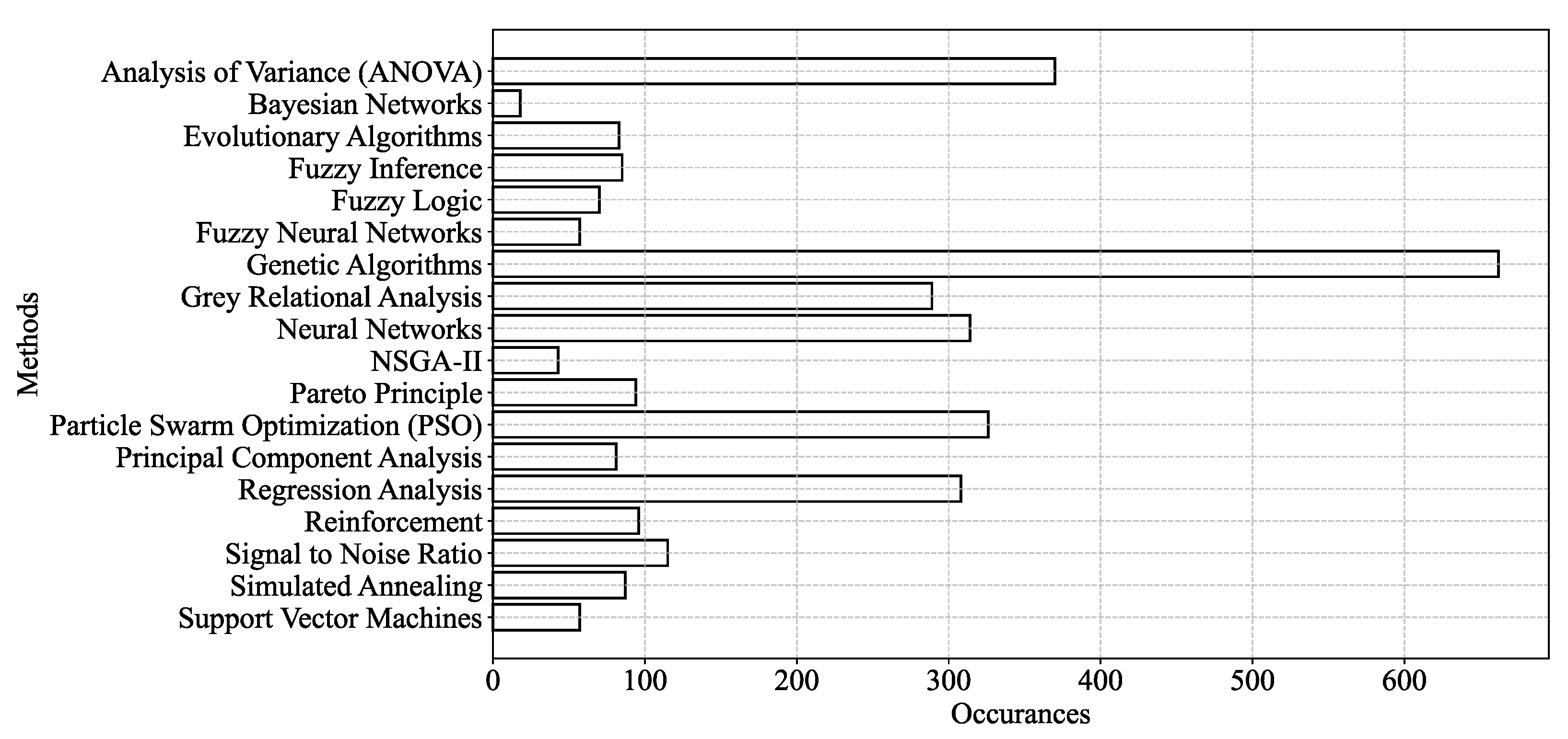
Figure A3.
Frequency of the considered machining processes.
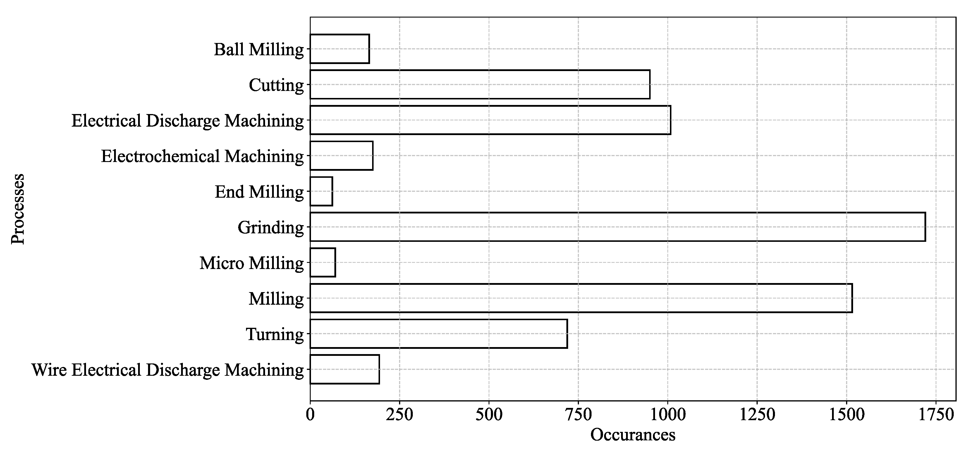
Figure A4.
Frequency of the considered parameters (CV-EVs).
Note that, while evaluating the occurrences of the keywords (Figure A2, Figure A3 and Figure A4), this study considered ‘Index Keywords’ rather than ‘Author Keywords’. The reason is that ‘Index Keywords’ provide a more structured way to analyze bibliographic data than ‘Author keywords’, because the latter vary significantly from person to person.
Appendix B: Access URL for Open Data
Access URL:
References
- Gupta, H.N. Manufacturing Process; 2nd ed.; New Age International Ltd: Daryaganj, New Delhi, 2009; ISBN 978-81-224-2844-5.
- Kalpakjian, S.; Schmid, S.R. Manufacturing Engineering and Technology; Eighth edition in SI units.; Pearson Education Limited: Harlow, 2023; ISBN 978-1-292-42224-4. [Google Scholar]
- Tlusty, J. Manufacturing Processes and Equipment; Prentice Hall: Upper Saddle River, NJ, 2000; ISBN 978-0-201-49865-3. [Google Scholar]
- Ullah, A.M.M.S. On the Interplay of Manufacturing Engineering Education and E-Learning. Int. J. Mech. Eng. Educ. 2016, 44, 233–254. [Google Scholar] [CrossRef]
- Ullah, A.M.M.S.; Harib, K.H. Manufacturing Process Performance Prediction by Integrating Crisp and Granular Information. J. Intell. Manuf. 2005, 16, 317–330. [Google Scholar] [CrossRef]
- Iwata, T.; Ghosh, A.K.; Ura, S. Toward Big Data Analytics for Smart Manufacturing: A Case of Machining Experiment. Proc. Int. Conf. Des. Concurr. Eng. Manuf. Syst. Conf. 2023, 2023, 33. [Google Scholar] [CrossRef]
- Ghosh, A.K.; Fattahi, S.; Ura, S. Towards Developing Big Data Analytics for Machining Decision-Making. J. Manuf. Mater. Process. 2023, 7, 159. [Google Scholar] [CrossRef]
- Kazuyuki, M. Survey of Big Data Use and Innovation in Japanese Manufacturing Firms (Online); 2025;
- Beckmann, B.; Giani, A.; Carbone, J.; Koudal, P.; Salvo, J.; Barkley, J. Developing the Digital Manufacturing Commons: A National Initiative for US Manufacturing Innovation. Procedia Manuf. 2016, 5, 182–194. [Google Scholar] [CrossRef]
- Kosarac, A.; Tabakovic, S.; Mladjenovic, C.; Zeljkovic, M.; Orasanin, G. Next-Gen Manufacturing: Machine Learning for Surface Roughness Prediction in Ti-6Al-4V Biocompatible Alloy Machining. J. Manuf. Mater. Process. 2023, 7, 202. [Google Scholar] [CrossRef]
- Perumal, S.; Amarnath, M.K.; Marimuthu, K.; Subramaniam, P.; Rathinavelu, V.; Jagadeesh, D. Titanium Carbonitride–Coated CBN Insert Featured Turning Process Parameter Optimization during AA359 Alloy Machining. Int. J. Adv. Manuf. Technol. 2025, 136, 45–56. [Google Scholar] [CrossRef]
- Teimouri, R.; Amini, S.; Mohagheghian, N. Experimental Study and Empirical Analysis on Effect of Ultrasonic Vibration during Rotary Turning of Aluminum 7075 Aerospace Alloy. J. Manuf. Process. 2017, 26, 1–12. [Google Scholar] [CrossRef]
- Agarwal, S.; Suman, R.; Bahl, S.; Haleem, A.; Javaid, M.; Sharma, M.K.; Prakash, C.; Sehgal, S.; Singhal, P. Optimisation of Cutting Parameters during Turning of 16MnCr5 Steel Using Taguchi Technique. Int. J. Interact. Des. Manuf. IJIDeM 2024, 18, 2055–2066. [Google Scholar] [CrossRef]
- Chen, L.; Li, J.; Ma, Z.; Jiang, C.; Yu, T.; Gu, R. Grinding Performance and Parameter Optimization of Laser DED TiC Reinforced Ni-Based Composite Coatings. J. Manuf. Process. 2025, 134, 466–481. [Google Scholar] [CrossRef]
- Banerjee, A.; Maity, K. Hybrid Optimization Strategies for Improved Machinability of Nitronic-50 with MT-PVD Inserts. J. Manuf. Process. 2025, 137, 221–251. [Google Scholar] [CrossRef]
- Kechagias, J. Multiparameter Signal-to-Noise Ratio Optimization for End Milling Cutting Conditions of Aluminium Alloy 5083. Int. J. Adv. Manuf. Technol. 2024, 132, 4979–4988. [Google Scholar] [CrossRef]
- Fattahi, S.; Ullah, A.S. Optimization of Dry Electrical Discharge Machining of Stainless Steel Using Big Data Analytics. Procedia CIRP 2022, 112, 316–321. [Google Scholar] [CrossRef]
- Chowdhury, M.A.K.; Ullah, A.M.M.S.; Anwar, S. Drilling High Precision Holes in Ti6Al4V Using Rotary Ultrasonic Machining and Uncertainties Underlying Cutting Force, Toolwear, and Production Inaccuracies. Materials 2017, 10, 1069. [Google Scholar] [CrossRef]
- Mongan, P.G.; Hinchy, E.P.; O’Dowd, N.P.; McCarthy, C.T.; Diaz-Elsayed, N. An Ensemble Neural Network for Optimising a CNC Milling Process. J. Manuf. Syst. 2023, 71, 377–389. [Google Scholar] [CrossRef]
- Bouhali, R.; Bendjeffal, H.; Chetioui, K.B.; Bousba, I. Multivariable Optimization Based on the Taguchi Method to Study the Cutting Conditions in Aluminum Turning. Int. J. Interact. Des. Manuf. IJIDeM 2024. [Google Scholar] [CrossRef]
- Usgaonkar, G.G.S.; Gaonkar, R.S.P. GRA and CoCoSo Based Analysis for Optimal Performance Decisions in Sustainable Grinding Operation. Int. J. Math. Eng. Manag. Sci. 2025, 10, 1–21. [Google Scholar] [CrossRef]
- R, M.K.; Ranganathan, R.; A, S.; Velu, R.; Jatti, V.S.; Mohan, D.G.; Vijayakumar, P. Achieving Multi-Response Optimization of Control Parameters for Wire-EDM on Additive Manufactured AlSi10Mg Alloy Using Taguchi-Grey Relational Theory. Eng. Res. Express 2025, 7, 015404. [Google Scholar] [CrossRef]
- Agarwal, D.; Yadav, S.; Singh, R.K.; Sharma, A.K. To Investigate the Effect of Discharge Energy and Addition of Nano-Powder on Processing of Micro Slots Using EDM Assisted µ-Milling Operation. Mater. Manuf. Process. 2025, 40, 80–94. [Google Scholar] [CrossRef]
- Fan, L.; Yang, G.; Zhang, Y.; Gao, L.; Wu, B. A Novel Tolerance Optimization Approach for Compressor Blades: Incorporating the Measured out-of-Tolerance Error Data and Aerodynamic Performance. Aerosp. Sci. Technol. 2025, 158, 109920. [Google Scholar] [CrossRef]
- Boga, C.; Koroglu, T. Proper Estimation of Surface Roughness Using Hybrid Intelligence Based on Artificial Neural Network and Genetic Algorithm. J. Manuf. Process. 2021, 70, 560–569. [Google Scholar] [CrossRef]
- Karthick, M.; Anand, P.; Siva Kumar, M.; Meikandan, M. Exploration of MFOA in PAC Parameters on Machining Inconel 718. Mater. Manuf. Process. 2022, 37, 1433–1445. [Google Scholar] [CrossRef]
- Kantheti, P.R.; Meena, K.L.; Chekuri, R.B.R. Maximizing Machining Efficiency and Quality in AA7075/Gr/B4 C HMMCs through Advanced DS-EDM Parameter Optimization Strategies. Eng. Res. Express 2024, 6, 045504. [Google Scholar] [CrossRef]
- Gangwar, S.; Mondal, S.C.; Kumar, A.; Ghadai, R.K. Performance Analysis and Optimization of Machining Parameters Using Coated Tungsten Carbide Cutting Tool Developed by Novel S3P Coating Method. Int. J. Interact. Des. Manuf. IJIDeM 2024, 18, 3909–3922. [Google Scholar] [CrossRef]
- Wan, L.; Chen, Z.; Zhang, X.; Wen, D.; Ran, X. A Multi-Sensor Monitoring Methodology for Grinding Wheel Wear Evaluation Based on INFO-SVM. Mech. Syst. Signal Process. 2024, 208, 111003. [Google Scholar] [CrossRef]
- Fu, X.; Li, K.; Zheng, M.; Wang, C.; Chen, E. Research on Dynamic Characteristics of Turning Process System Based on Finite Element Generalized Dynamics Space. Int. J. Adv. Manuf. Technol. 2024, 131, 4683–4698. [Google Scholar] [CrossRef]
- Cai, M.; Chen, M.; Gong, Y.; Gong, Q.; Zhu, T.; Zhang, M. Optimizing Grinding Parameters for Surface Integrity in Single Crystal Nickel Superalloys Using SVM Modeling. Int. J. Adv. Manuf. Technol. 2024, 135, 315–335. [Google Scholar] [CrossRef]
- Mohanta, D.K.; Sahoo, B.; Mohanty, A.M. Experimental Analysis for Optimization of Process Parameters in Machining Using Coated Tools. J. Eng. Appl. Sci. 2024, 71, 38. [Google Scholar] [CrossRef]
- Pathapalli, V.R.; Pittam, S.R.; Sarila, V.; Burragalla, D.; Gagandeep, A. Multi-Objective Parametric Optimization of AWJM Process Using Taguchi-Based GRA and DEAR Methodology. Proc. Inst. Mech. Eng. Part E J. Process Mech. Eng. 2024, 238, 2845–2853. [Google Scholar] [CrossRef]
- Chan, T.-C.; Wu, S.-C.; Ullah, A.; Farooq, U.; Wang, I.-H.; Chang, S.-L. Integrating Numerical Techniques and Predictive Diagnosis for Precision Enhancement in Roller Cam Rotary Table. Int. J. Adv. Manuf. Technol. 2024, 132, 3427–3445. [Google Scholar] [CrossRef]
- Tanvir, M.H.; Hussain, A.; Rahman, M.M.T.; Ishraq, S.; Zishan, K.; Rahul, S.T.T.; Habib, M.A. Multi-Objective Optimization of Turning Operation of Stainless Steel Using a Hybrid Whale Optimization Algorithm. J. Manuf. Mater. Process. 2020, 4, 64. [Google Scholar] [CrossRef]
- Wang, Z.; Zhang, T.; Yu, T.; Zhao, J. Assessment and Optimization of Grinding Process on AISI 1045 Steel in Terms of Green Manufacturing Using Orthogonal Experimental Design and Grey Relational Analysis. J. Clean. Prod. 2020, 253, 119896. [Google Scholar] [CrossRef]
- Mohanta, D.K.; Sahoo, B.; Mohanty, A.M. Optimization of Process Parameter in AI7075 Turning Using Grey Relational, Desirability Function and Metaheuristics. Mater. Manuf. Process. 2023, 38, 1615–1625. [Google Scholar] [CrossRef]
- Chanie, S.E.; Bogale, T.M.; Siyoum, Y.B. Optimization of Wire-Cut EDM Parameters Using Artificial Neural Network and Genetic Algorithm for Enhancing Surface Finish and Material Removal Rate of Charging Handlebar Machining from Mild Steel AISI 1020. Int. J. Adv. Manuf. Technol. 2025, 136, 3505–3523. [Google Scholar] [CrossRef]
- Wang, J.; Liu, H.; Qi, X.; Wang, Y.; Ma, W.; Zhang, S. Tool Wear Prediction Based on SVR Optimized by Hybrid Differential Evolution and Grey Wolf Optimization Algorithms. CIRP J. Manuf. Sci. Technol. 2024, 55, 129–140. [Google Scholar] [CrossRef]
- Tamang, S.K.; Chauhan, A.; Banerjee, D.; Teyi, N.; Samanta, S. Developing Precision in WEDM Machining of Mg-SiC Nanocomposites Using Machine Learning Algorithms. Eng. Res. Express 2024, 6, 045435. [Google Scholar] [CrossRef]
- Painuly, M.; Singh, R.P.; Trehan, R. Investigation into Electrochemical Machining of Aviation Grade Inconel 625 Super Alloy: An Experimental Study with Advanced Optimization and Microstructural Analysis. Aircr. Eng. Aerosp. Technol. 2025, 97, 137–148. [Google Scholar] [CrossRef]
- Mahanti, R.; Das, M. Sustainable EDM Production of Micro-Textured Die-Surfaces: Modeling and Optimizing the Process Using Machine Learning Techniques. Measurement 2025, 242, 115775. [Google Scholar] [CrossRef]
- Wang, Y.; Xu, H.; Ou, Z.; Liu, J.; Wang, G. Analysis of Root Residual Stress and Total Tooth Profile Deviation in Hobbing and Investigation of Optimal Parameters. CIRP J. Manuf. Sci. Technol. 2025, 58, 20–39. [Google Scholar] [CrossRef]
- Nguyen, V.-H.; Le, T.-T.; Nguyen, A.-T.; Hoang, X.-T.; Nguyen, N.-T.; Nguyen, N.-K. Optimization of Milling Conditions for AISI 4140 Steel Using an Integrated Machine Learning-Multi Objective Optimization-Multi Criteria Decision Making Framework. Measurement 2025, 242, 115837. [Google Scholar] [CrossRef]
- Guidetti, X.; Rupenyan, A.; Fassl, L.; Nabavi, M.; Lygeros, J. Plasma Spray Process Parameters Configuration Using Sample-Efficient Batch Bayesian Optimization. In Proceedings of the 2021 IEEE 17th International Conference on Automation Science and Engineering (CASE); IEEE: Lyon, France, August 23, 2021; pp. 31–38. [Google Scholar]
- Ao, S.; Xiang, S.; Yang, J. A Hyperparameter Optimization-Assisted Deep Learning Method towards Thermal Error Modeling of Spindles. ISA Trans. 2025, 156, 434–445. [Google Scholar] [CrossRef]
- Kumar, S.; Dvivedi, A.; Tiwari, T.; Tewari, M. Predictive Modeling of Tool Wear in Rotary Tool Micro-Ultrasonic Machining. Proc. Inst. Mech. Eng. Part E J. Process Mech. Eng. 2024, 238, 2160–2172. [Google Scholar] [CrossRef]
- Bousnina, K.; Hamza, A.; Yahia, N.B. Design of an Intelligent Simulator ANN and ANFIS Model in the Prediction of Milling Performance (QCE) of Alloy 2017A. Artif. Intell. Eng. Des. Anal. Manuf. 2024, 38, e23. [Google Scholar] [CrossRef]
- Ullah, A.M.M.S.; Harib, K.H. A Human-Assisted Knowledge Extraction Method for Machining Operations. Adv. Eng. Inform. 2006, 20, 335–350. [Google Scholar] [CrossRef]
- Saleem, M.Q.; Mehmood, A. Eco-Friendly Precision Turning of Superalloy Inconel 718 Using MQL Based Vegetable Oils: Tool Wear and Surface Integrity Evaluation. J. Manuf. Process. 2022, 73, 112–127. [Google Scholar] [CrossRef]
- Sun, W.; Zhang, Y.; Luo, M.; Zhang, Z.; Zhang, D. A Multi-Criteria Decision-Making System for Selecting Cutting Parameters in Milling Process. J. Manuf. Syst. 2022, 65, 498–509. [Google Scholar] [CrossRef]
- Leese, M. The New Profiling: Algorithms, Black Boxes, and the Failure of Anti-Discriminatory Safeguards in the European Union. Secur. Dialogue 2014, 45, 494–511. [Google Scholar] [CrossRef]
- d’Alessandro, B.; O’Neil, C.; LaGatta, T. Conscientious Classification: A Data Scientist’s Guide to Discrimination-Aware Classification. Big Data 2017, 5, 120–134. [Google Scholar] [CrossRef]
- Emmert-Streib, F.; Yli-Harja, O.; Dehmer, M. Artificial Intelligence: A Clarification of Misconceptions, Myths and Desired Status. Front. Artif. Intell. 2020, 3, 524339. [Google Scholar] [CrossRef]
- Bzdok, D.; Altman, N.; Krzywinski, M. Statistics versus Machine Learning. Nat. Methods 2018, 15, 233–234. [Google Scholar] [CrossRef]
- Tabachnick, B.G.; Fidell, L.S. Using Multivariate Statistics; Always learning; 6. ed., international ed.; Pearson: Boston Munich, 2013; ISBN 978-0-205-89081-1.
- Miller, R.G.; Brown, B.W. Beyond ANOVA: Basics of Applied Statistics; Chapman & Hall texts in statistical science series; 1st ed.; Chapman & Hall: London ; New York, 1997; ISBN 978-0-412-07011-2.
- Dang, X.; Al-Rahawi, M.; Liu, T.; Mohammed, S.T.A. Single and Multi-Response Optimization of Scroll Machining Parameters by the Taguchi Method. Int. J. Precis. Eng. Manuf. 2024, 25, 1601–1614. [Google Scholar] [CrossRef]
- Igwe, N.C.; Ozoegwu, C.G. Analyzing Empirically and Optimizing Surface Roughness and Tool Wear during Turning Aluminum Matrix/Rice Husk Ash (RHA) Composite. Int. J. Adv. Manuf. Technol. 2024, 134, 1563–1580. [Google Scholar] [CrossRef]
- Zhujani, F.; Abdullahu, F.; Todorov, G.; Kamberov, K. Optimization of Multiple Performance Characteristics for CNC Turning of Inconel 718 Using Taguchi–Grey Relational Approach and Analysis of Variance. Metals 2024, 14, 186. [Google Scholar] [CrossRef]
- Muthukrishnan, N.; Davim, J.P. Optimization of Machining Parameters of Al/SiC-MMC with ANOVA and ANN Analysis. J. Mater. Process. Technol. 2009, 209, 225–232. [Google Scholar] [CrossRef]
- Sureshkumar, B.; Navaneethakrishnan, G.; Panchal, H.; Manjunathan, A.; Prakash, C.; Shinde, T.; Mutalikdesai, S.; Prajapati, V.V. Effects of Machining Parameters on Dry Turning Operation of Nickel 200 Alloy. Int. J. Interact. Des. Manuf. IJIDeM 2024, 18, 6023–6038. [Google Scholar] [CrossRef]
- Azawqari, A.A.; Amrani, M.A.; Hezam, L.; Baggash, M.; Abidin, Z.Z. Multi-Objectives Optimization of WEDM Parameters on Machining of AISI 304 Based on Taguchi Method. Int. J. Adv. Manuf. Technol. 2024, 134, 5493–5510. [Google Scholar] [CrossRef]
- Pal, S.; Malviya, S.K.; Pal, S.K.; Samantaray, A.K. Optimization of Quality Characteristics Parameters in a Pulsed Metal Inert Gas Welding Process Using Grey-Based Taguchi Method. Int. J. Adv. Manuf. Technol. 2009, 44, 1250–1260. [Google Scholar] [CrossRef]
- Singh, J.; Gill, S.S.; Mahajan, A. Experimental Investigation and Optimizing of Turning Parameters for Machining of Al7075-T6 Aerospace Alloy for Reducing the Tool Wear and Surface Roughness. J. Mater. Eng. Perform. 2024, 33, 8745–8756. [Google Scholar] [CrossRef]
- Xie, Y.; Chang, G.; Yang, J.; Zhao, M.; Li, J. Process Optimization of Robotic Polishing for Mold Steel Based on Response Surface Method. Machines 2022, 10, 283. [Google Scholar] [CrossRef]
- Zadeh, L.A. Fuzzy Sets as a Basis for a Theory of Possibility. Fuzzy Sets Syst. 1999, 100, 9–34. [Google Scholar] [CrossRef]
- Dubois, D.; Foulloy, L.; Mauris, G.; Prade, H. Probability-Possibility Transformations, Triangular Fuzzy Sets, and Probabilistic Inequalities. Reliab. Comput. 2004, 10, 273–297. [Google Scholar] [CrossRef]
- Sharif Ullah, A.M.M.; Shamsuzzaman, M. Fuzzy Monte Carlo Simulation Using Point-Cloud-Based Probability–Possibility Transformation. SIMULATION 2013, 89, 860–875. [Google Scholar] [CrossRef]
- Mauris, G.; Lasserre, V.; Foulloy, L. A Fuzzy Approach for the Expression of Uncertainty in Measurement. Measurement 2001, 29, 165–177. [Google Scholar] [CrossRef]
- Ullah, A.; Shahinur, S.; Haniu, H. On the Mechanical Properties and Uncertainties of Jute Yarns. Materials 2017, 10, 450. [Google Scholar] [CrossRef]
- Shahinur, S.; Ullah, A.S. Quantifying the Uncertainty Associated with the Material Properties of a Natural Fiber. Procedia CIRP 2017, 61, 541–546. [Google Scholar] [CrossRef]
- Ullah, A.M.M. Surface Roughness Modeling Using Q-Sequence. Math. Comput. Appl. 2017, 22, 33. [Google Scholar] [CrossRef]
- Sharif Ullah, A.M.M.; Fuji, A.; Kubo, A.; Tamaki, J.; Kimura, M. On the Surface Metrology of Bimetallic Components. Mach. Sci. Technol. 2015, 19, 339–359. [Google Scholar] [CrossRef]
- Ullah, A.M.M.S. A.M.M.S. A Fuzzy Monte Carlo Simulation Technique for Sustainable Society Scenario (3S) Simulator. In Sustainability Through Innovation in Product Life Cycle Design; Matsumoto, M., Masui, K., Fukushige, S., Kondoh, S., Eds.; EcoProduction; Springer Singapore: Singapore, 2017; pp. 601–618. ISBN 978-981-10-0469-8. [Google Scholar]
- Ghosh, A.K.; Ullah, A.S.; Teti, R.; Kubo, A. Developing Sensor Signal-Based Digital Twins for Intelligent Machine Tools. J. Ind. Inf. Integr. 2021, 24, 100242. [Google Scholar] [CrossRef]
- On the Full and Open Exchange of Scientific Data; National Academies Press: Washington, D.C., 1995; p. 18769; ISBN 978-0-309-30427-6.
- Orlowski, C. Smart Cities and Open Data. In Management of IOT Open Data Projects in Smart Cities; Elsevier, 2021; pp. 1–41 ISBN 978-0-12-818779-1.
Figure 1.
Context of optimization in machining.
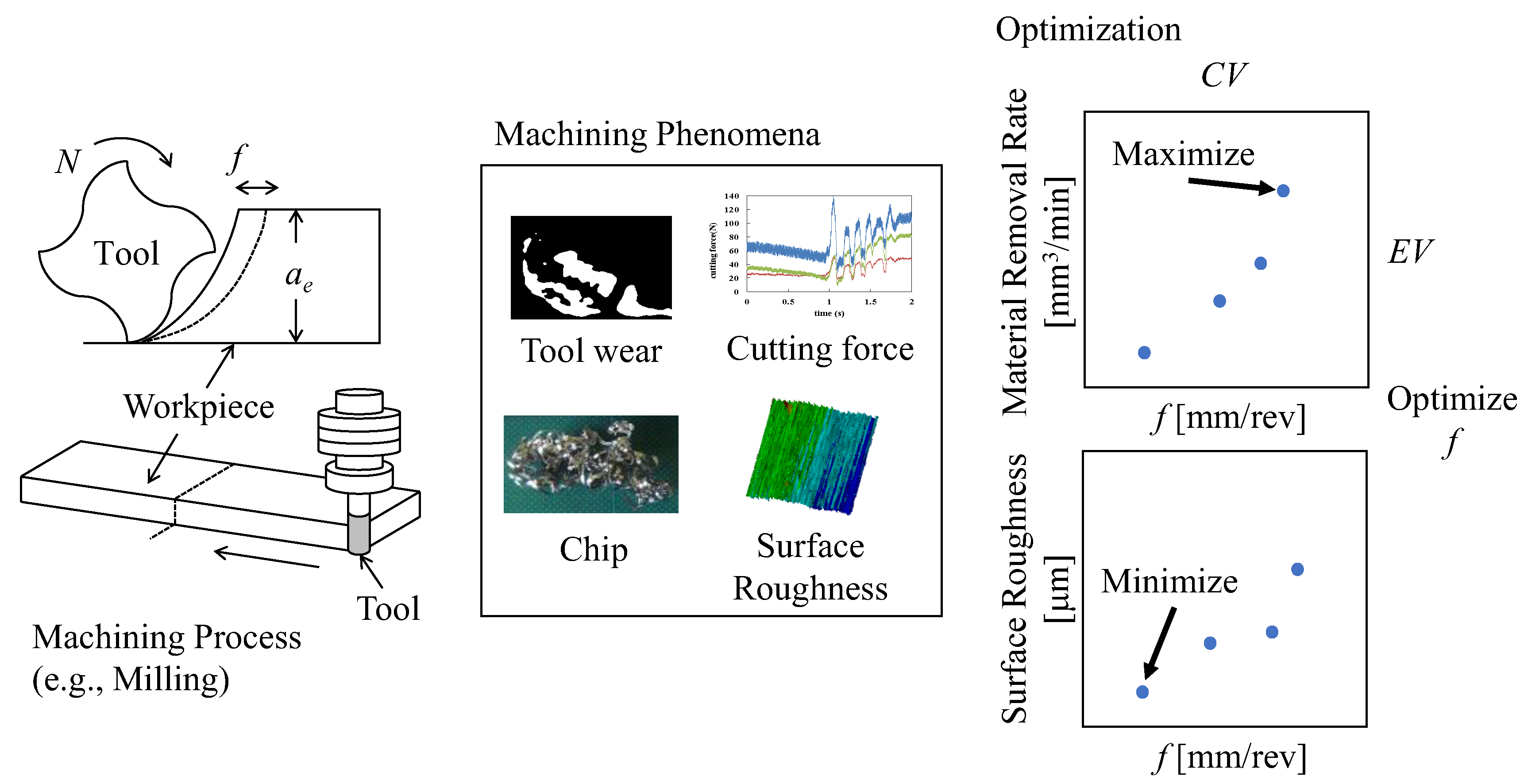
Figure 2.
Open data lifecycle.
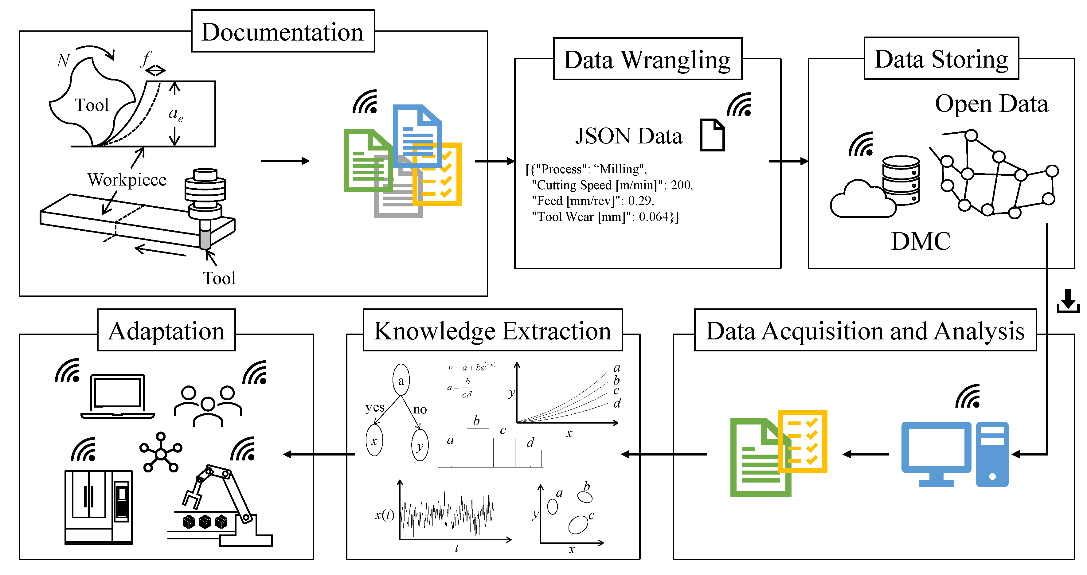
Figure 5.
A given set of numerical data.
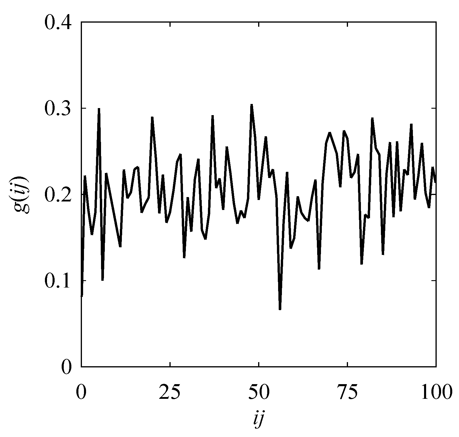
Figure 6.
Relative position of A and B in the point -cloud (g_((ij) ),g_(i+1)j).
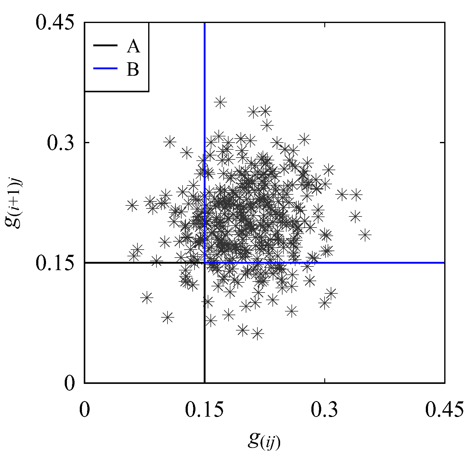
Figure 7.
The typical nature of Pr_A(g) and Pr_B(g) for unimodal quantity.
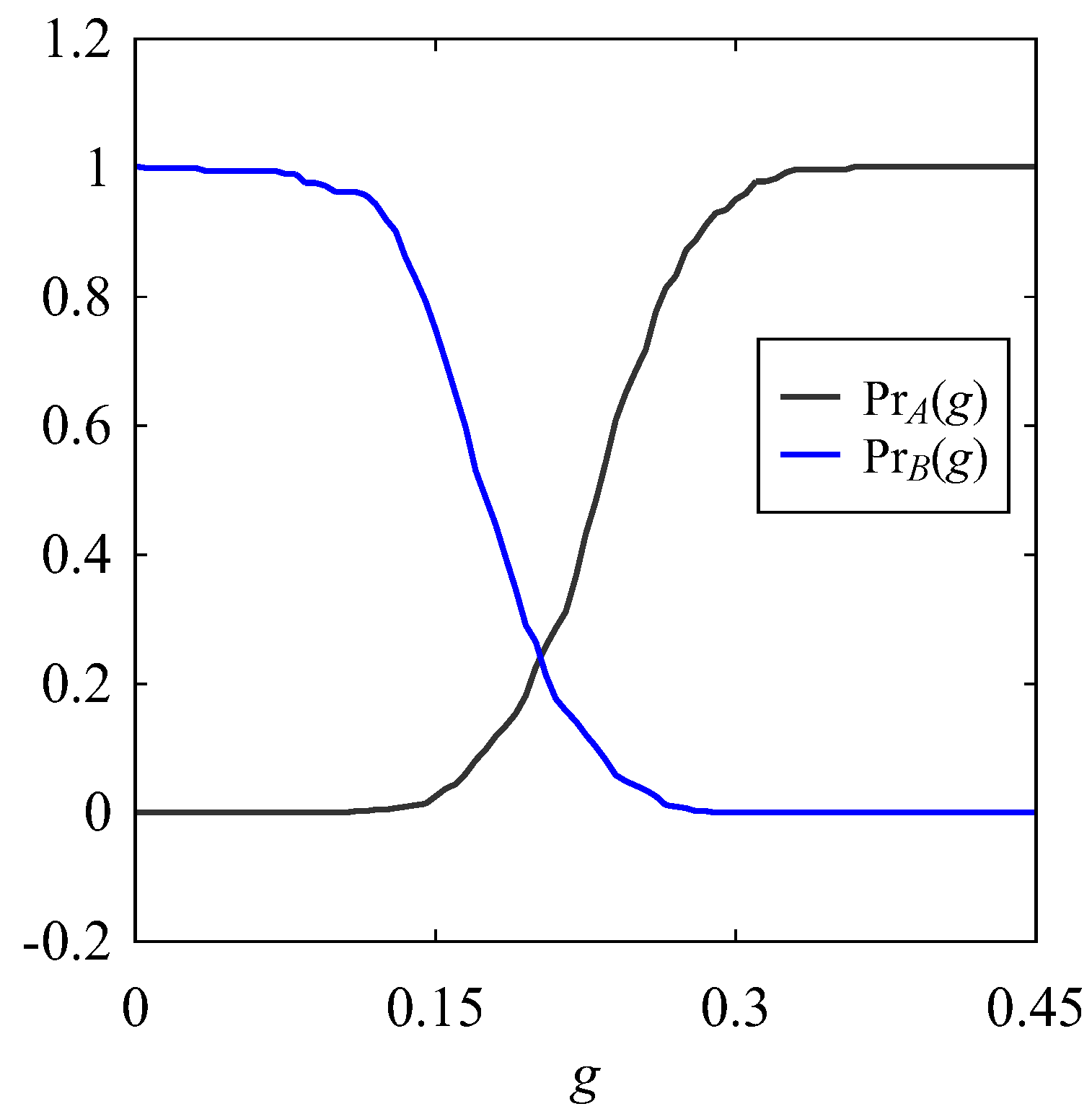
Figure 8.
Nature of Pr_A(g)+ Pr_B(g) and min(Pr_A(g), Pr_B(g)) for unimodal data.
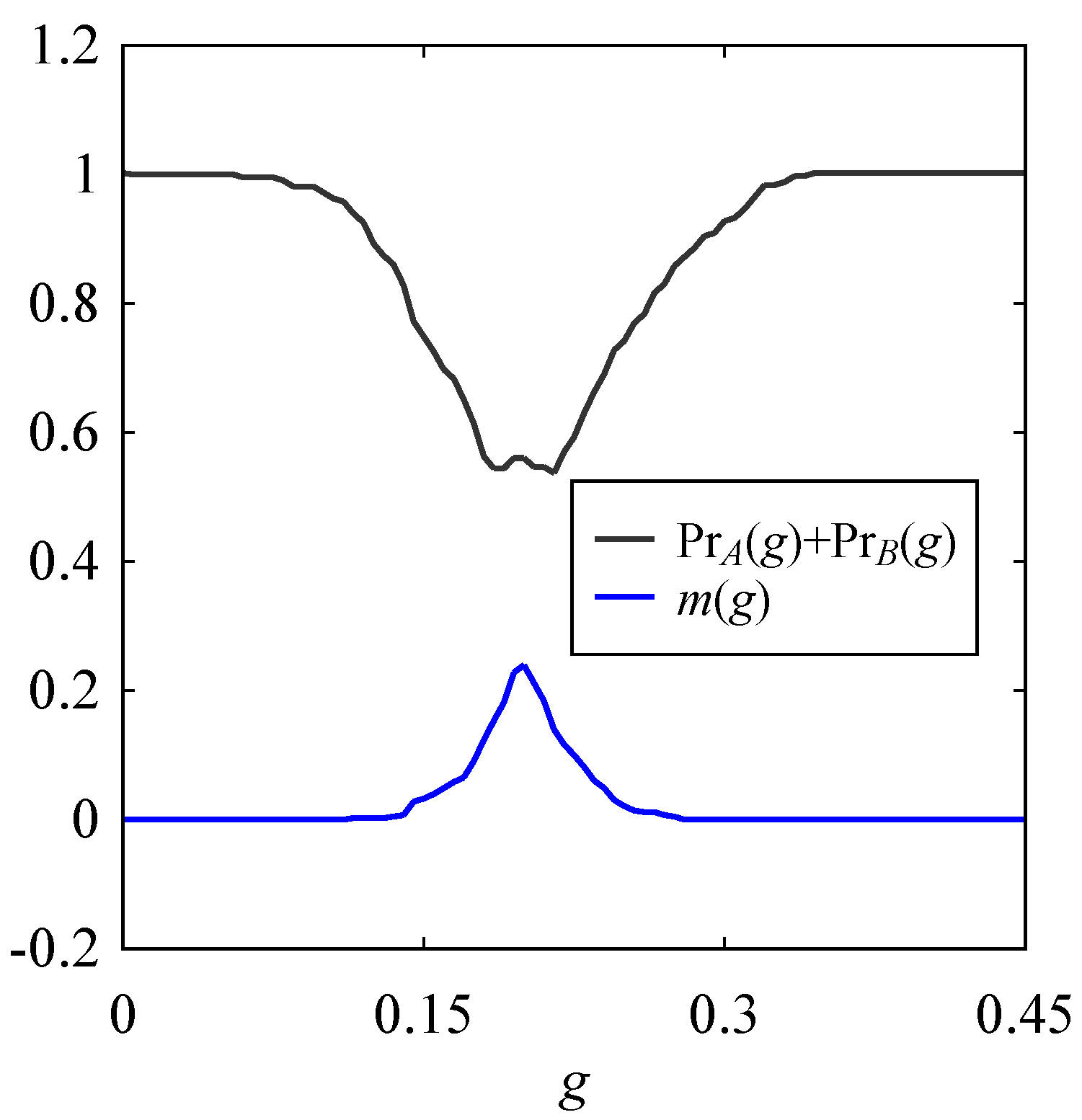
Figure 9.
Nature of cumulative probability distribution of a point cloud.
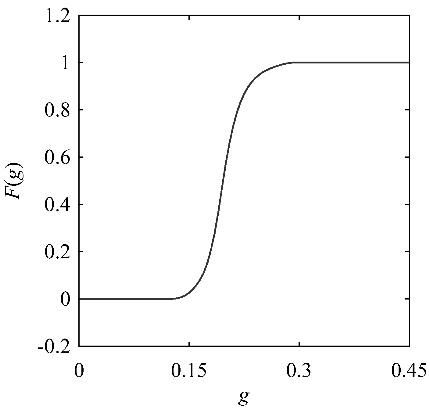
Figure 10.
The nature of probability distribution of a unimodal point-cloud.
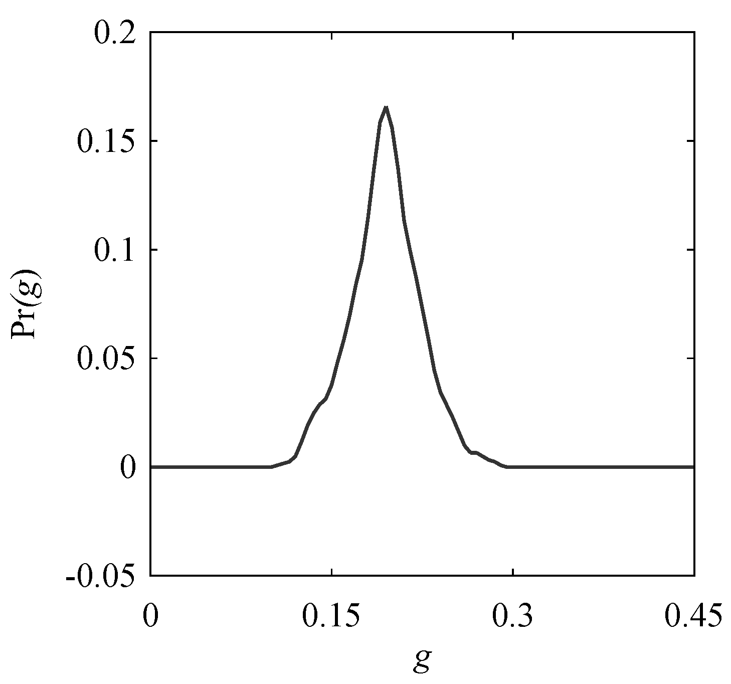
Figure 11.
The nature of possibility distribution of a unimodal point-cloud.
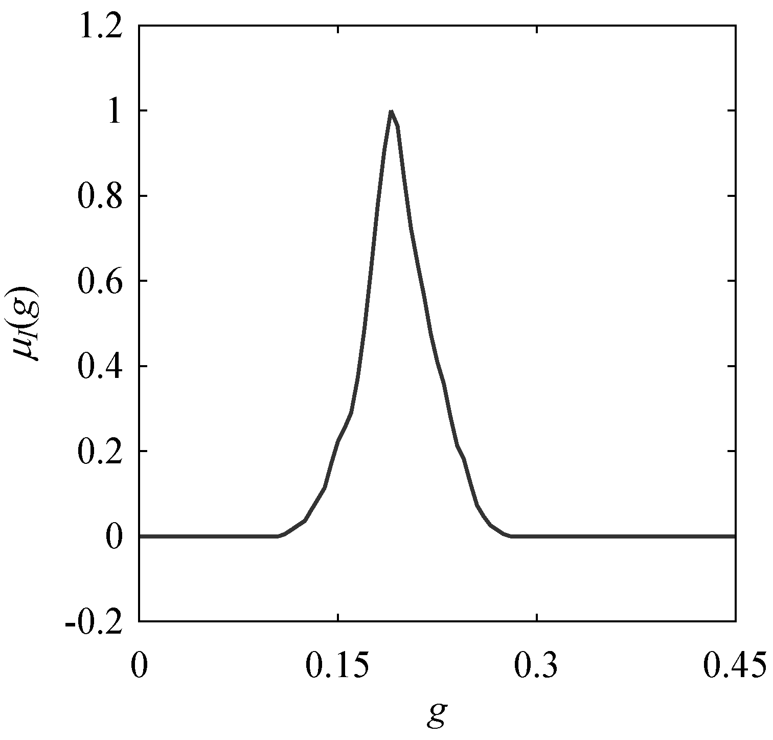
Figure 12.
Induced triangular fuzzy number from possibility distribution.
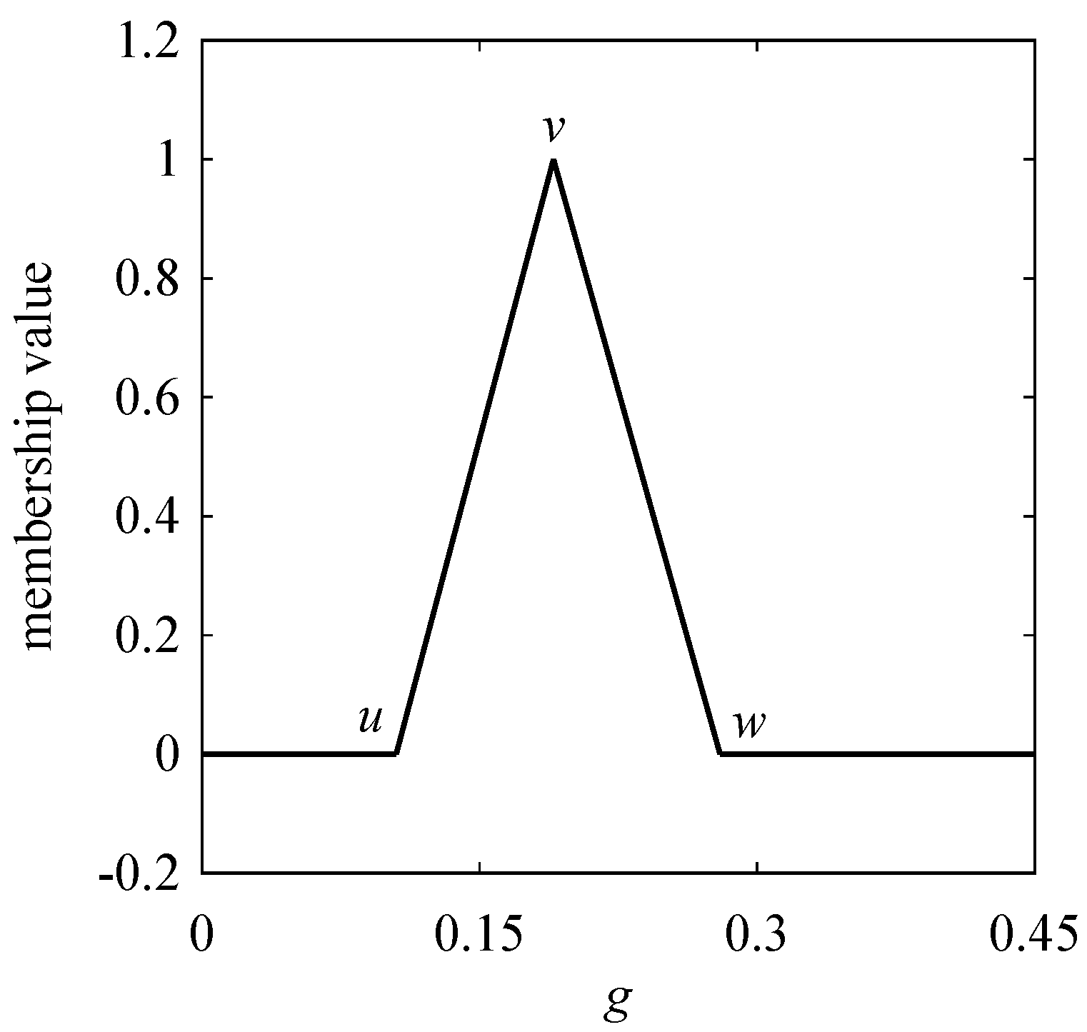
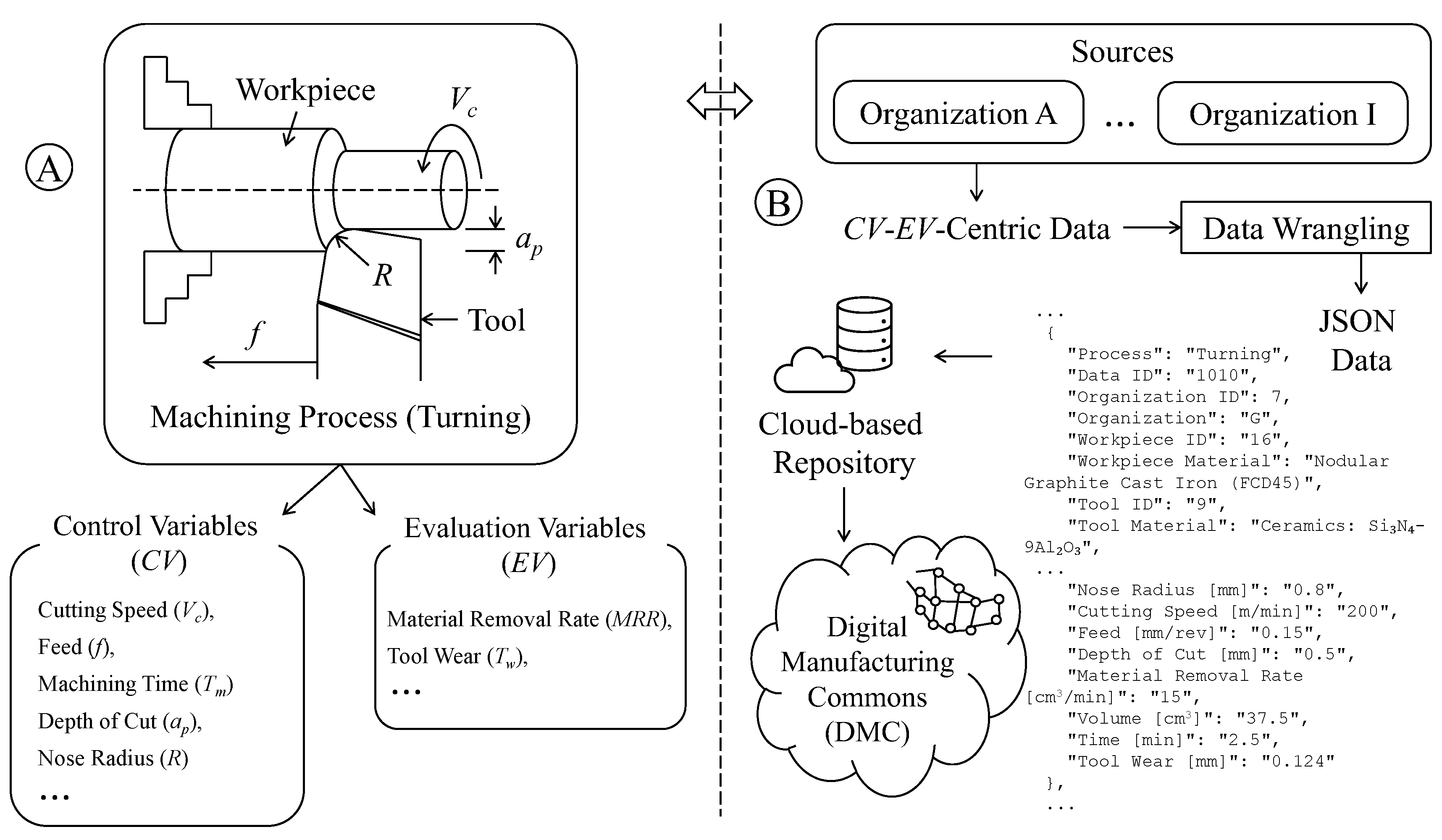
Figure 14.
A visualization of the CV-EV-centric open data.
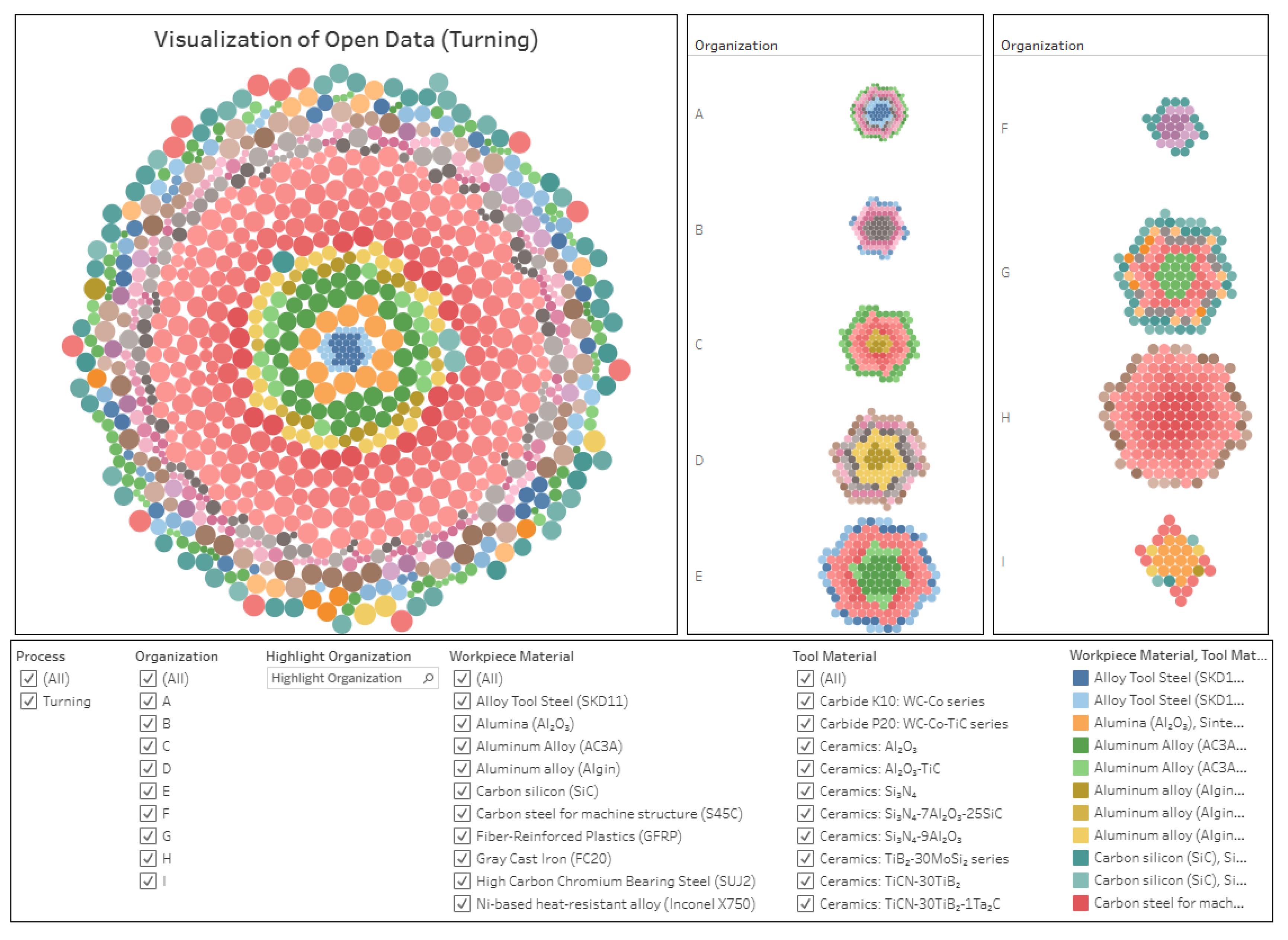
Figure 15.
Open data relevant to the workpiece-tool combination considering Carbon steel for machine structure (S45C) and Cermet: TiN-TaN (WM1-TM1).
Figure 15.
Open data relevant to the workpiece-tool combination considering Carbon steel for machine structure (S45C) and Cermet: TiN-TaN (WM1-TM1).
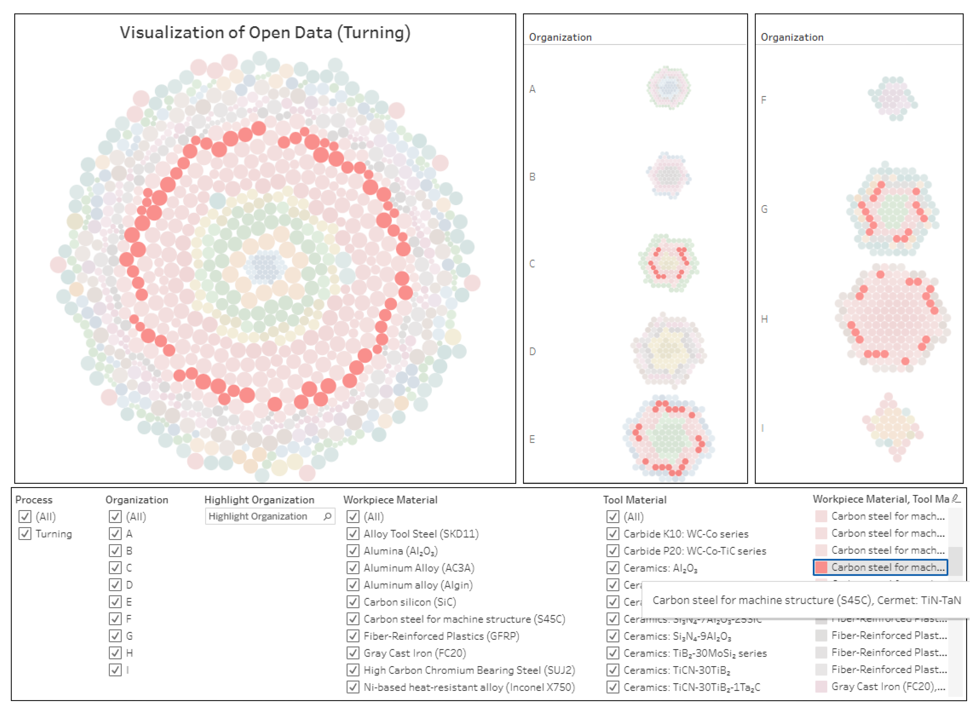
Figure 16.
Open data relevant to the workpiece-tool combination considering Carbon steel for machine structure (S45C) and Ceramics: TiCN-30TiB2-1TaN (WM1-TM2).
Figure 16.
Open data relevant to the workpiece-tool combination considering Carbon steel for machine structure (S45C) and Ceramics: TiCN-30TiB2-1TaN (WM1-TM2).
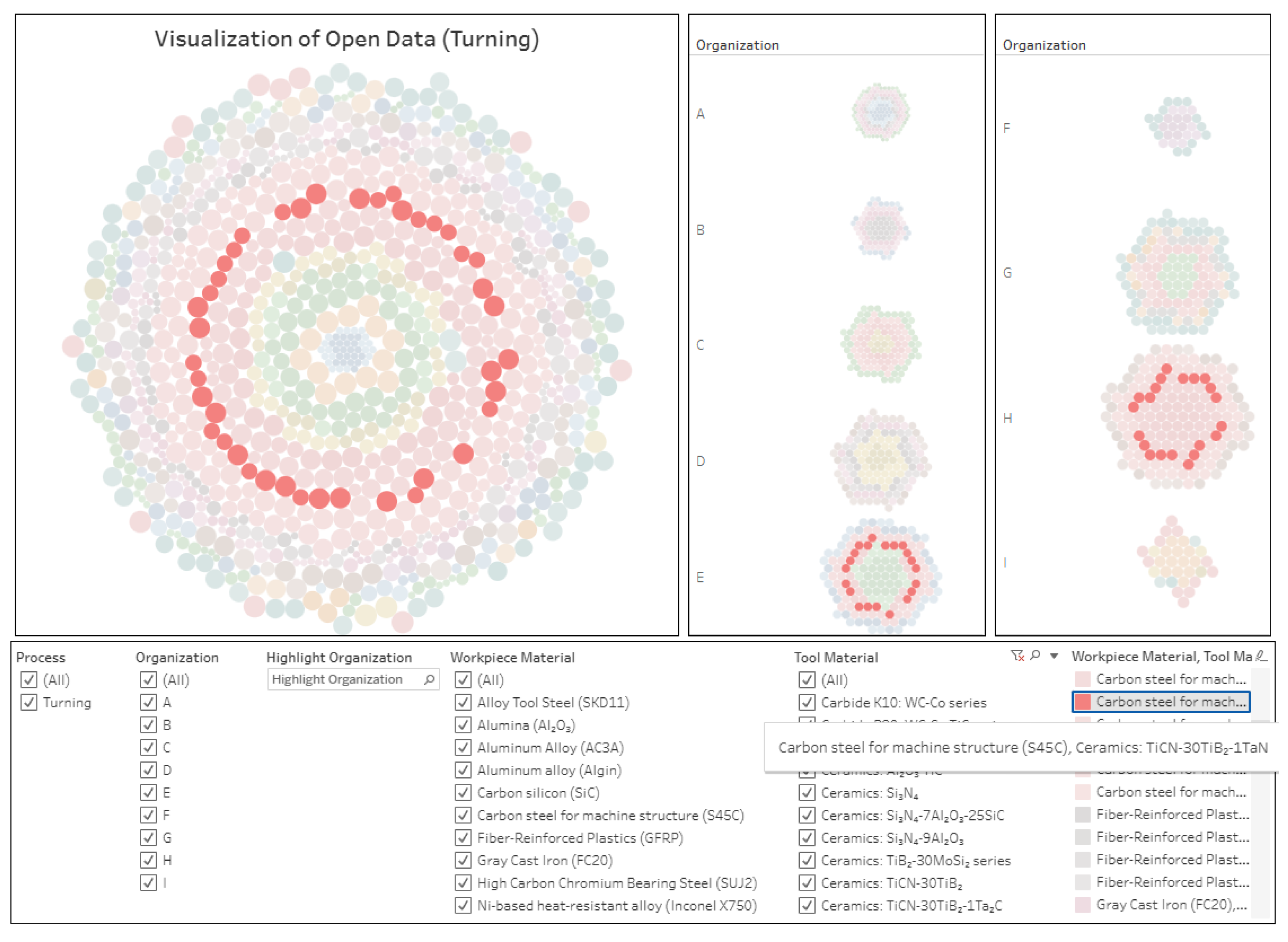
Figure 17.
Results from SNR for TM1. (a) Effect of vc on Tw, (b) Effect of f on Tw, and (c) Effect of Tm on Tw.
Figure 17.
Results from SNR for TM1. (a) Effect of vc on Tw, (b) Effect of f on Tw, and (c) Effect of Tm on Tw.
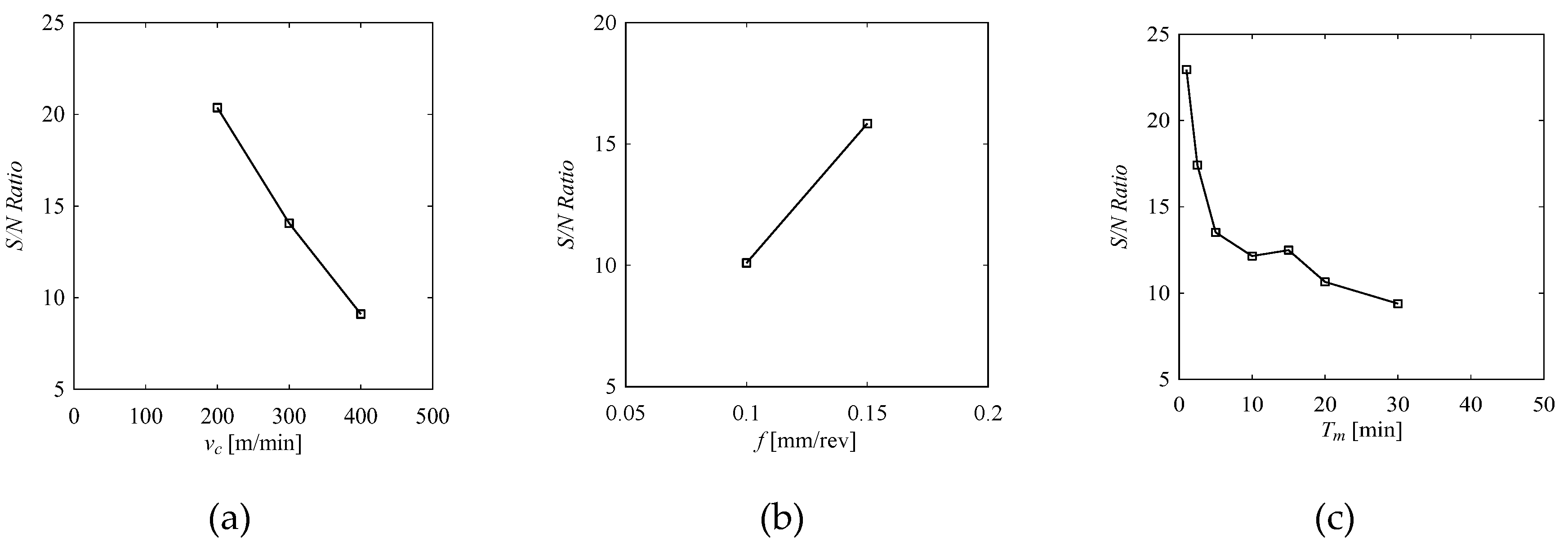
Figure 18.
Results from PD for TM1. (a) Effect of vc on Tw, (b) Effect of f on Tw, and (c) Effect of Tm on Tw.
Figure 18.
Results from PD for TM1. (a) Effect of vc on Tw, (b) Effect of f on Tw, and (c) Effect of Tm on Tw.
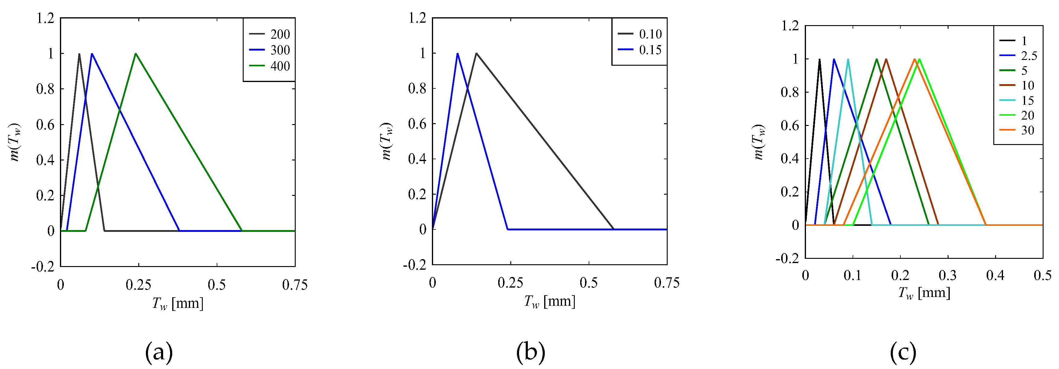
Figure 19.
Results from SNR for TM2. (a) Effect of vc on Tw, (b) Effect of f on Tw, and (c) Effect of Tm on Tw.
Figure 19.
Results from SNR for TM2. (a) Effect of vc on Tw, (b) Effect of f on Tw, and (c) Effect of Tm on Tw.
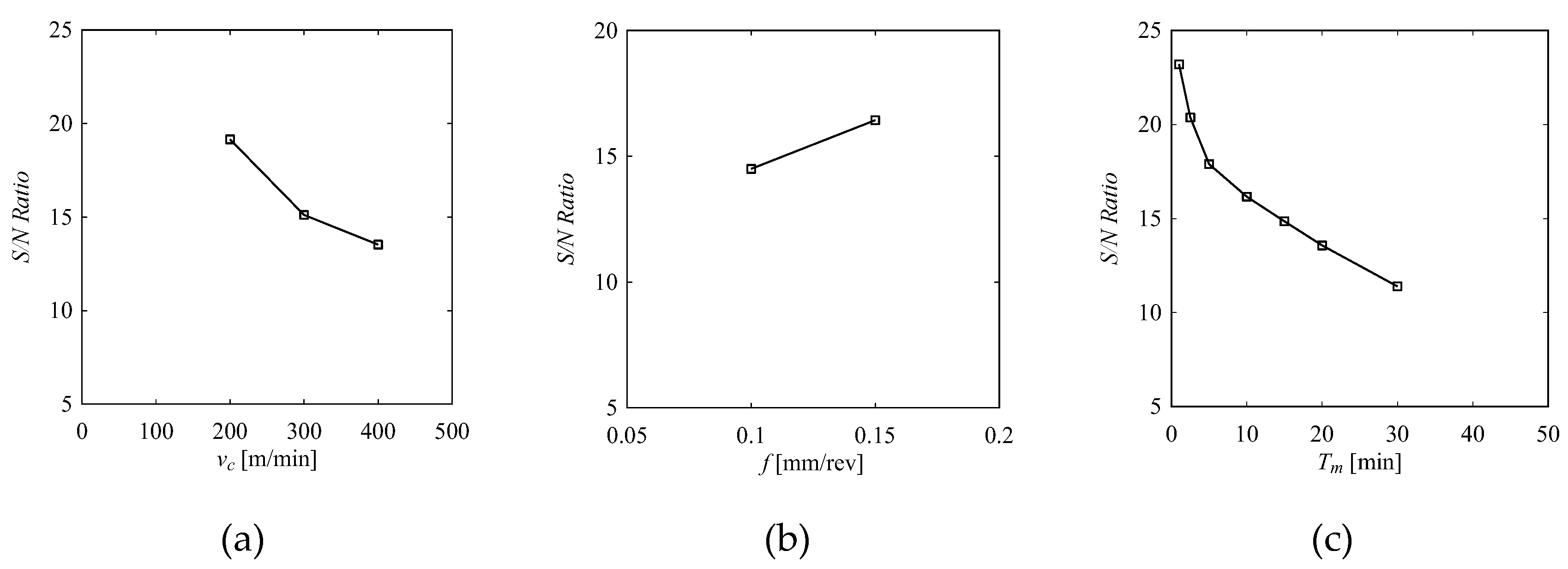
Figure 20.
Results from PD for TM2. (a) Effect of vc on Tw, (b) Effect of f on Tw, and (c) Effect of Tm on Tw.
Figure 20.
Results from PD for TM2. (a) Effect of vc on Tw, (b) Effect of f on Tw, and (c) Effect of Tm on Tw.
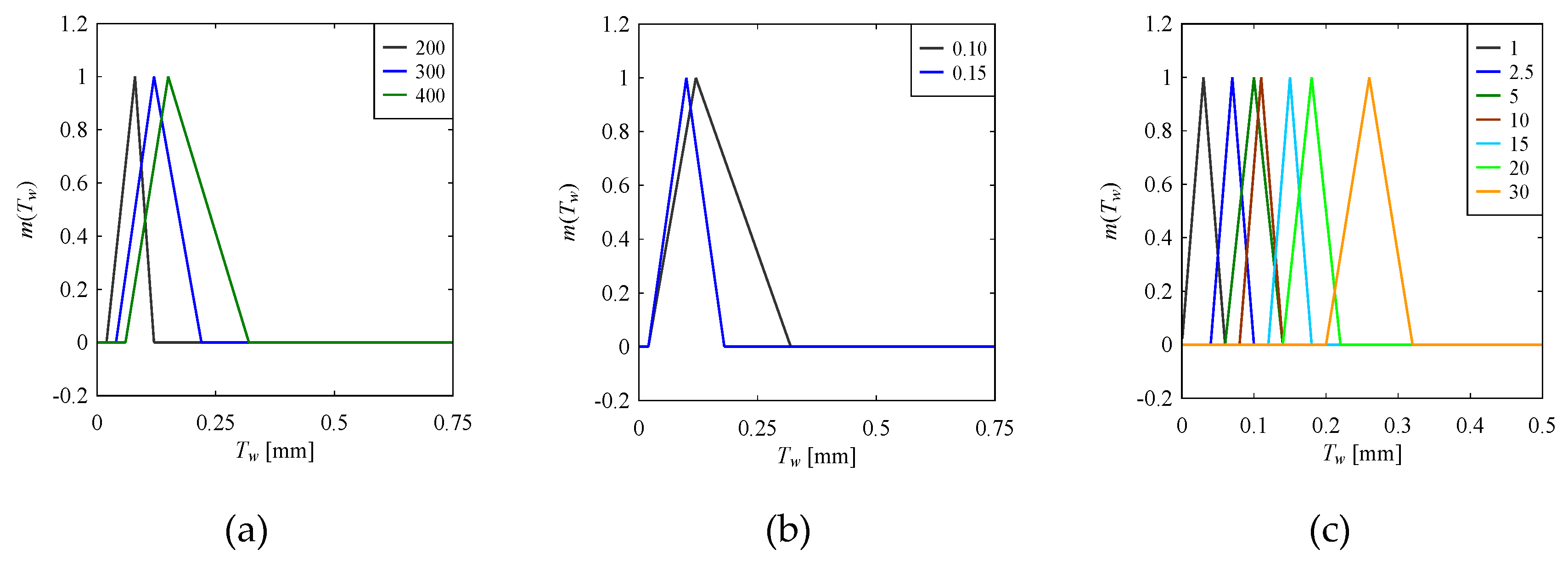
Figure 21.
Quantified average tool wear (Tw) and its variability with machining time (Tm) for WM1-TM2. (a) Average Tw from the centroid (Cx) of each TFN. (b) Variability in Tw from the spread (S) of each TFN.
Figure 21.
Quantified average tool wear (Tw) and its variability with machining time (Tm) for WM1-TM2. (a) Average Tw from the centroid (Cx) of each TFN. (b) Variability in Tw from the spread (S) of each TFN.
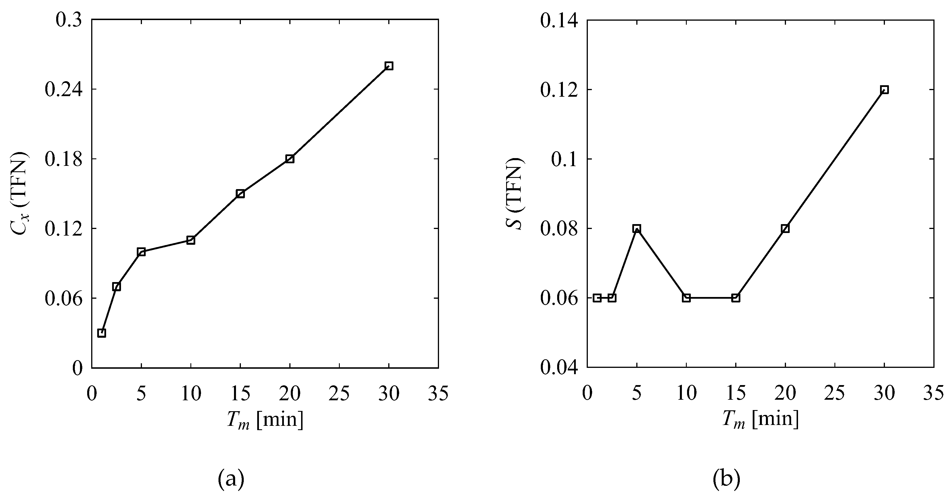
Figure 22.
Quantified average tool wear (Tw) and its variability with machining time (Tm) for WM1-TM1. (a) Average Tw from the centroid (Cx) of each TFN. (b) Variability in Tw from the spread (S) of each TFN.
Figure 22.
Quantified average tool wear (Tw) and its variability with machining time (Tm) for WM1-TM1. (a) Average Tw from the centroid (Cx) of each TFN. (b) Variability in Tw from the spread (S) of each TFN.
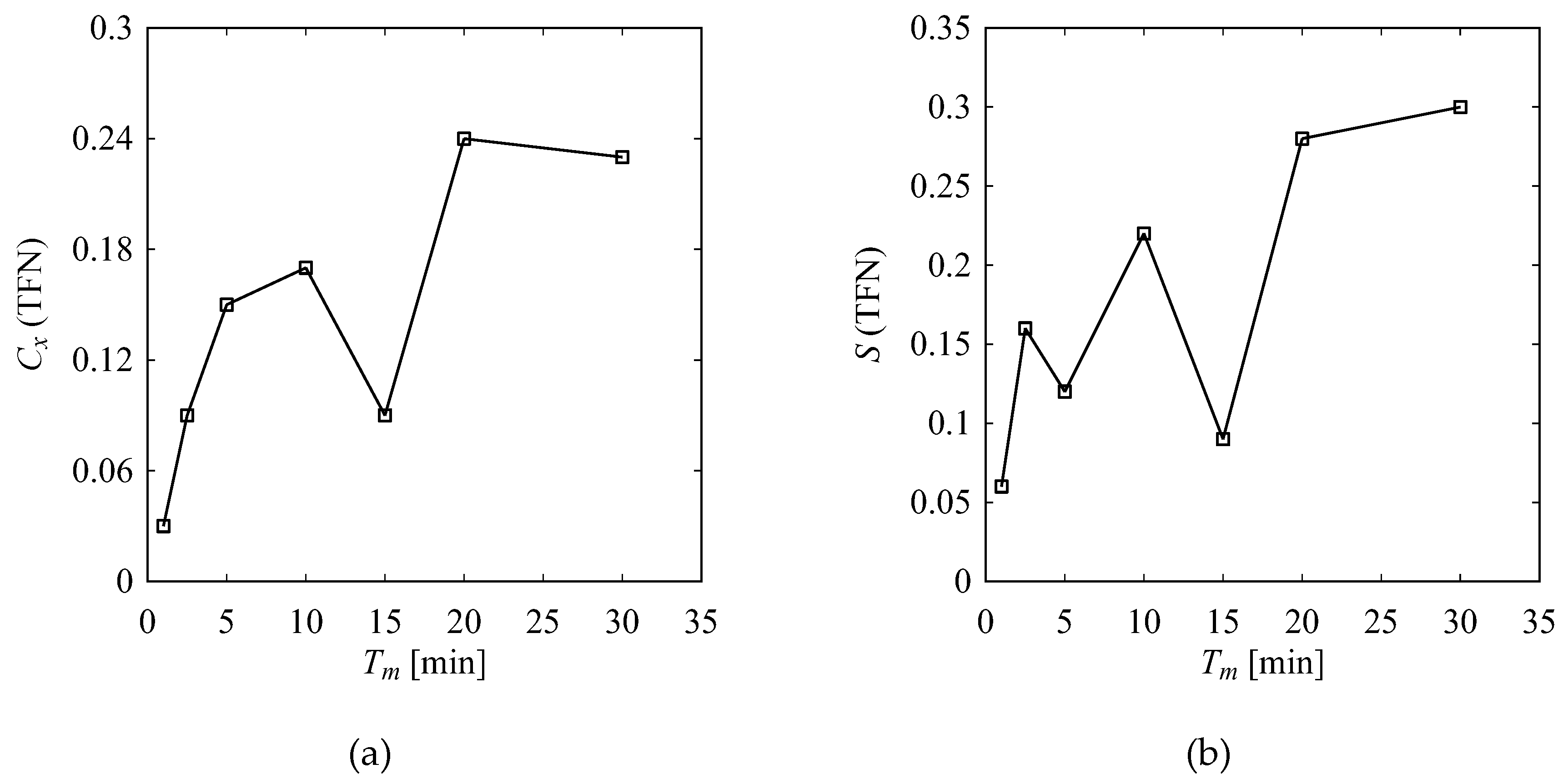
Figure A1.
Number of journal articles from 2000 to 2024.
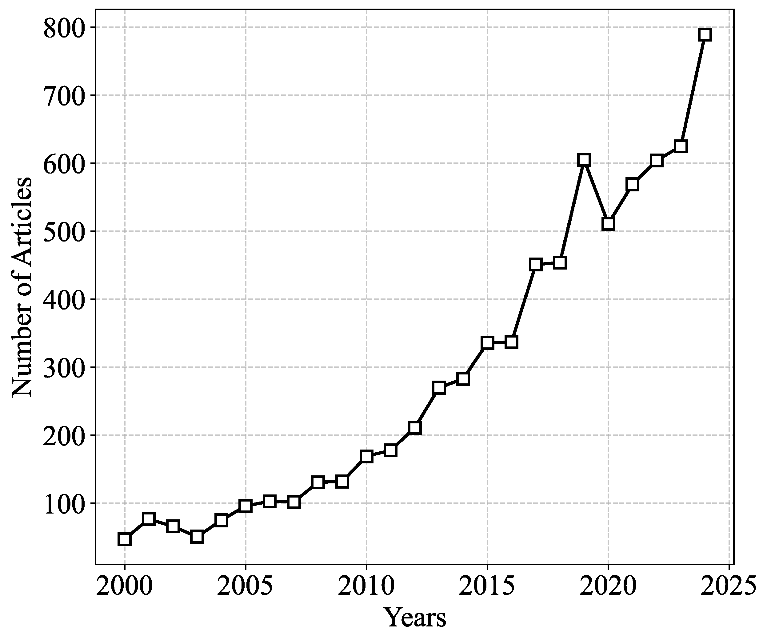

Table 1.
Workpiece materials in the open data.
| ID | Name of Workpiece Material | Number of Data |
| WM1 | Carbon steel for machine structure (S45C) | 289 |
| WM2 | Gray Cast Iron (FC20) | 142 |
| WM3 | Fiber-Reinforced Plastics (GFRP) | 103 |
| WM4 | Pure titanium (Ti) | 90 |
| WM5 | Ni-based heat-resistant alloys (Inconel 600) | 65 |
| WM6 | Ni-based heat-resistant alloy (Inconel X750) | 64 |
| WM7 | Stainless Steel (SUS304) | 55 |
| WM8 | Aluminum Alloy (AC3A) | 50 |
| WM9 | Aluminum alloy (Algin) | 50 |
| WM10 | Alloy Tool Steel (SKD11) | 42 |
| WM11 | High Carbon Chromium Bearing Steel (SUJ2) | 17 |
| WM12 | Nodular Graphite Cast Iron (FCD45) | 14 |
| WM13 | Alumina (Al2O3) | 13 |
| WM14 | Zirconia (ZrO2) | 12 |
| WM15 | Silicon nitrogen (Si3N4) | 4 |
| WM16 | Carbon silicon (SiC) | 3 |
Table 2.
Tool materials for Carbon steel for machine structure (S45C) in open data.
| Workpiece Material | ID | Name of Tool Material | Number of Data |
| Carbon steel for machine structure (S45C), denoted as WM1 |
TM1 | Cermet: TiN-TaN | 68 |
| TM2 | Ceramics: TiCN-30TiB2-1TaN | 42 | |
| TM3 | Ceramics: TiCN-30TiB2-1Ta₂C | 40 | |
| TM4 | Coating: Al2O3 | 38 | |
| TM5 | Ceramics: TiCN-30TiB2 | 21 | |
| TM6 | Ceramics: TiN-30TiB2 | 21 | |
| TM7 | Coating: TiCN | 21 | |
| TM8 | Ceramics: Al2O3 | 15 | |
| TM9 | Ceramics: TiB2-30MoSi2 series | 13 | |
| TM10 | Ceramics: Si3N4-9Al2O3 | 7 | |
| TM11 | Ceramics: Si3N4-7Al2O3-25Si | 3 |
Table 3.
Outlining the Control and Evaluation variables (CV-EV).
| Variable Types | Name of CVs | States |
| Control Variable (CVs) | Cutting Speed (vc) [m/min] | 200, 300, 400 |
| Feed (f) [mm/rev] | 0.1, 0.15 | |
| Machining Time (Tm) [min] | 1, 2.5, 5, 10,15, 20, 30 | |
| Evaluation Variable (EV) | Tool Wear (Tw) [mm] |
Table 4.
Results from ANOVA for TM1.
| CVs | Source of Variation | df | MS | F-value | P-value | Significant / Nonsignificant |
| vc | Between Groups | 2 | 0.225 | 16.75 | 1.4E-6 | Significant |
| Within Groups | 65 | 0.013 | ||||
| f | Between Groups | 1 | 0.178 | 10.24 | 0.002 | Significant |
| Within Groups | 66 | 0.017 | ||||
| Tm | Between Groups | 6 | 0.047 | 2.76 | 0.019 | Significant |
| Within Groups | 61 | 0.017 |
Table 5.
Results from ANOVA for TM2.
| CVs | Source of Variation | df | MS | F-value | P-value | Significant / Nonsignificant |
| vc | Between Groups | 2 | 0.029 | 5.901 | 0.006 | Significant |
| Within Groups | 39 | 0.005 | ||||
| f | Between Groups | 1 | 0.007 | 1.170 | 0.286 | Nonsignificant |
| Within Groups | 40 | 0.006 | ||||
| Tm | Between Groups | 6 | 0.026 | 9.211 | 4.56E-6 | Significant |
| Within Groups | 35 | 0.003 |
Disclaimer/Publisher’s Note: The statements, opinions and data contained in all publications are solely those of the individual author(s) and contributor(s) and not of MDPI and/or the editor(s). MDPI and/or the editor(s) disclaim responsibility for any injury to people or property resulting from any ideas, methods, instructions or products referred to in the content. |
© 2025 by the authors. Licensee MDPI, Basel, Switzerland. This article is an open access article distributed under the terms and conditions of the Creative Commons Attribution (CC BY) license (http://creativecommons.org/licenses/by/4.0/).
Copyright: This open access article is published under a Creative Commons CC BY 4.0 license, which permit the free download, distribution, and reuse, provided that the author and preprint are cited in any reuse.


