Submitted:
18 February 2025
Posted:
19 February 2025
You are already at the latest version
Abstract
6D pose estimation of unknown objects is an unsolved research problem in computer vision. This contribution proposes a novel method for estimating an object's pose using a monocular camera and an artificially created point cloud from the geometric object data. Point cloud generation and pose estimation are done with deep learning methods, combining several neural network-based approaches in one system. This paper describes the architecture and methods and compares and evaluates several ideas.
Keywords:
3D object detection
; 6D pose estimation
; machine learning
; computer vision
; image processing
; convolutional neural network
1. Introduction and Motivation
Estimating the position and orientation (6D pose) of three-dimensional objects in camera images is a fundamental problem for many applications and a base for several follow-up algorithms. It offers significant advantages in manufacturing, autonomous driving, and humanoid robotics disciplines. Especially in industrial robotics, the 6D pose estimation is a prerequisite to solving the bin-picking problem [1]. Another important application area are humanoid robots. These robots are expected to be used in both factories and home environments, requiring them to recognize and grasp several and potentially unknown objects [2].
From an algorithmic perspective, recent 6D object pose estimation approaches can be classified into learning-based and non-learning-based methods [3]. Learning-based techniques commonly utilize convolutional neural networks and can be further classified into bounding box prediction, classification-based, and regression-based methods [4]. Other modern approaches include segmentation-driven estimation [5], dense 3D object coordinate labeling, and dense 2D-3D correspondences [6]. Multi-view consistency has been explored to improve accuracy [7], while efficient center voting strategies have been developed for 3D point clouds [8].
Traditional methods are commonly based upon classical point cloud registration techniques, e.g., the well-known iterative close point (ICP) algorithm, in combination with template matching methods and previously known 3D models (given by CAD models or similar).
In our contribution, we want to address a special field of application where the 3D model of the object to be detected is not known beforehand. This means the object must be detected, segmented, and transformed into a three-dimensional representation. The result can then be used to track the object within a sequence of images, which is very useful in sim2-real robotics problems. An estimate of friction coefficients or other important parameters is possible given a precise orientation and position.
The two most important points to emphasize are: First, we present a framework for 6D pose estimation without retraining or finetuning an existing neural network for given or new objects. Second, no prerendering or use of given 3D models is needed. We explore different deep leanring based architectures and combinations of networks to detect objects, gain 3D point cloud approximations and subsequently give a 6D estimate of the object.
Therefore, we want to present the related work to clarify the differences and improvements in our approach. Afterward, we describe different steps in the evolution of our approach, highlighting the pros and cons of each architectural choice and setup. We developed an individual loss function for the given problem and presented several network types, such as simple regression-based approaches, convolutional networks, and transformer-based architectures. We present exemplary results for the proposed systems and evaluate them based on efficiency, possible applications, and experimental results.
2. Related Work
The field of pose estimation and object detection encompasses extensive research, covering topics such as instance and category recognition, rigid and articulated objects, and coarse (quantized) and precise (6D) pose estimation. In the brief review below, we concentrate on methods specifically designed to detect instances of rigid objects in cluttered scenes while simultaneously estimating their 6D pose. Some of these approaches have already been discussed above.
2.1. Correlation-Based Methods
Early algorithms for 6D pose estimation relied on correlation-based methods, including the approach by Hinterstoisser et al. [9]. These methods evaluate gradients along object edges and surface normals within the target parts. The pose can be determined by matching the orientation and amplitude of the gradients with those of the CAD model using correlation.
Other approaches utilize SIFT or similar features and perform matching using PnP or modified ICP algorithms. However, more traditional methods are needed to solve the pose estimation problem [10] adequately.
2.2. Learning-Based Methods
Recent advancements in machine learning have enabled object recognition tasks to reach performance levels that surpass human capabilities. Consequently, applying these insights from object classification, detection, and segmentation to pose estimation is logical. The success of these methods is documented and proven by the line mod dataset [11], which is one of the unofficial quality measures for 6D pose estimation of natural objects.
Recent advancements have focused on learning-based methods, which can be categorized into instance-level and category-level approaches [12]. These methods have shown superior performance compared to traditional feature-based and template-based techniques [4]. Neural networks, such as CNNs, have been employed to learn object representations and compare observed and rendered images for accurate pose estimation [13]. Some approaches create synthetic images from limited real observations to improve training data [14]. Others utilize RGB-D images and point clouds for more robust estimation [15]. Challenges in 6D pose estimation include handling occlusions, symmetries, and varying lighting conditions [3,6]. Despite these challenges, learning-based methods have demonstrated state-of-the-art performance across various datasets and application scenarios, including robotic manipulation and autonomous driving [12,16].
Numerous derivatives of object detectors have been adapted for 6D pose estimation. Examples include SSD-6D [17], which employs a modified Inception V4 network, and the work by Tekin et al., which modifies a YOLO network [18]. A modified EfficcientNEt is used in [19] and achieves excellent results. Standalone CNN architectures, such as the one proposed in [20], have also been developed. Lately, transformer-based detectors have emerged; an example can be found in [21], where a modified DETR architecture is used.
However, these methods are typically limited to estimating the poses of known objects or objects the network has been trained upon.
2.3. Rendering-Based Methods
Rendering-based approaches are commonly employed to improve the accuracy of existing methods or estimate the pose of unknown objects. Various poses of the object are prerendered in these methods, and a neural network interpolates the desired pose in the image based on this data [9].
Recent research in 6D pose estimation for unknown objects has focused on rendering-based methods. Several approaches use neural networks to reconstruct and render latent 3D representations of objects from reference views [14]. These methods enable pose estimation for novel objects without retraining. Some techniques employ coarse-to-fine optimization strategies [22] or iterative refinement to improve accuracy [23]. Silhouette-based methods have shown promise for texture-less objects [24]. New datasets and metrics have been introduced to evaluate these approaches [25]. While most recent methods rely on deep learning, traditional feature-based approaches using point pair features on range data remain competitive [26]. Overall, rendering-based methods have demonstrated state-of-the-art performance on various benchmarks, offering a promising direction for generalizable 6D pose estimation of unknown objects.
Additionally, some approaches utilize renderers as refinement techniques to correct the estimated pose. Notable examples include the work in [7,27]. The latter method is also capable of estimating the pose of unknown objects. Both approaches are iterative, progressively refining the pose by rendering and comparing results in each step.
2.4. Additional Methods
Combinations of the methods mentioned above are frequently employed. Modern refinement approaches utilize ICP (Iterative Closest Point) and depth images. Additionally, alternative methods have been developed to address the problem using autoencoders [28,29]. These autoencoders generate an image in which the object is replaced by a color-coded 3D model, from which the pose can then be derived [30].
Segmentations are sometimes used as a foundation [13], though this also often involves autoencoders. One method, for instance, employs autoencoders to combine image segments with RGB-D data to identify the best correspondences with patches of the 3D model [13,31]. Furthermore, the publication in [7] proposes a method for pose estimation using images captured from multiple perspectives.
3. Proposed Approach
All current methods either require full retraining of the networks or some renderer for the relevant objects. This work aims to identify various objects and estimate their positions without requiring the network to be trained upon them or retrained (transfer learning) on chosen objects. The fundamental approach of this work is to leverage a large collection of 3D objects to learn the correspondence between 3D features and image features. Another source of inspiration is the research by DeTone et al. [32], where two images are fed into a CNN to estimate the relative homography between them. However, in our case, we want to find feature correspondences between 2D images and 3D objects. By utilizing large datasets, the network should be able to generalize to unseen objects.
Simple and fast-to-train architectures were used to assess the feasibility of this approach.
The following Sections describe the evaluation of the above-mentioned approach. The goal is to determine whether point clouds generated from 2D images are sufficient to estimate the pose of the objects. The focus was placed on developing and utilizing simple and efficient architectures to maintain low complexity and feasibility.
3.1. Dataset Creation
A dataset is always required to train a neural network. The general rule is that the larger, the better. However, in contrast to 2D image problems, where large datasets exist (e.g., the COCO data set with over 330,000 images), for 3D objects, leading datasets are relatively limited. Additionally, the diversity of possible objects is limited, which hinders a neural network’s ability to generalize effectively [33].
The dataset for evaluation and training consists of 40,000 objects from the ABC 3D dataset [34], split into 95% training and 5% test data, ensuring no overlap to test generalization on new objects. Objects were left untextured to simplify the proof of concept, focusing the network solely on geometric features without distraction. Textures and backgrounds were omitted to avoid complicating training, as they cannot be derived from the point cloud.
For training, the objects were rendered in 32 different rotations, allowing the model to learn the significance of rotation for 3D objects. The corresponding pose for each rotation was stored in a Pandas file. To simplify the process, the objects were centered in the image with their centroid at the origin, and no translation was applied. The centering of the point clouds was performed as follows: First, the centroid of the point cloud was calculated.
where is the coordinates of the ith point, and is the total number of points in the point cloud. The scaling factor is then calculated:
where represents the Euclidean norm.
Finally, the points were normalized:
The points can now be placed with the center of gravity in the middle of the image and rotated around it, which results in faster mesh convergence. A point cloud with Points is sampled for each rotation, which means that 32-point clouds exist for each object. This is to ensure variation of the points so that the network does not overfit to the specific position.
The images were rendered at a resolution of pixels using the Hard Phong shader from PyTorch3D.
Exemplary renderings are shown in Figure 1.
3.2. Training Workflow and Hardware
A local hardware system was set up to allow for later ease of implementation. A Linux operating system with a Docker container of the Google Colab environment is used as software. The GPU is a medium-sized Nvidia RTX 3090 with 12 GB of RAM. The system is accessed via SSH port forwarding to allow for evaluation in the browser of a client PC. This environment can easily be extended to the cloud version of Colab if larger models are to be trained.
3.3. Regression Network Approach
The regression network approach represents the simplest method of combining the point cloud with an image. The basic idea is to extract and combine features from the image and the point cloud and use a simple multi-layer perceptron (MLP) for pose regression.
The main focus is on the network’s capabilities to generalize new, unknown objects and their limitations.
3.3.1. Architecture
The feature network was chosen from the state of the art as EfficientNet from Google [35]. This architecture is characterized by its ease of use, high performance, few parameters, and low computational cost. The low complexity was the main selection criterion for this network, as fast results are desirable, and only limited resources are available in real-world application scenarios. The smallest trainable version of EfficientNet works with input images of pixels and processes them into a feature vector of . For the feature extraction from the point cloud, the PointNet architecture is chosen [36]. This network’s simple structure achieves convincing results in classification and segmentation tasks in 3D applications. PointNet can work with point clouds of different sizes and generates a feature vector with classification entries.
In a subsequent step, the two feature vectors are combined, and the regression of the pose is applied to the combined representation. In the final layer of the network, a pose regression with a dimension of is performed. In addition, the network has a second output that enables the regression of translational parameters. The hyperbolic tangent (TanH) was chosen as an activation function for the rotation, as the six values shall be mapped between the set limits . A linear layer was used for the translational parameters. All other layers use ReLU activations. The structure of the resulting network and setup for this approach is shown in Figure 2 as abstract high-level architecture.
3.3.2. Evaluation
A suitable error function was required to train the neural network and evaluate its performance. Since the objects used are often rotationally and mirror-symmetrically arranged, the absolute distance between corresponding points is not always meaningful as an error measure.
Let and be two-point clouds with corresponding points. The error function for calculating the mean absolute distance between the corresponding points of the two-point clouds is defined as:
where and are the coordinates of the corresponding points in the point clouds and , and is the Euclidean norm.
An error function based on the nearest neighbor point (KNN) was used to reduce the effects of symmetries. This considers deviations along the axis of rotation for symmetrical parts and has less influence on the final result:
Convergence with this error function is often slow, and many local minima can occur. For this reason, the L1 loss (mean absolute error) between the estimated and true rotations was also calculated. This value is less meaningful for symmetrical objects but can help the network to converge better:
where represents the predicted values, and represents the actual target values. The weighting in the learning process is:
Only was used for the evaluation and the plots, as this is the easiest to interpret. The learning curve is shown in Figure 3. Exemplary extracts of the estimates on the validation data set, which consists of unknown objects, can also be seen in Figure 4.
It is visible that the result could be better. However, the network can estimate the pose of unknown objects. The loss displayed above the objects is the L2 loss, which is why it is so small.
3.4. Rendering Approximator Autoencoder
After the initial tests for pose regression with features showed feasibility, the system must be integrated into a detector architecture that recognizes the objects in images and generates the 3D point cloud. The main challenge with this is combining features and object detections within the input images. We propose three different methods to combine the information, which are presented in the following Sections.
3.4.1. Point Net Architecture
The basic architecture is inspired by U-Net, whose effectiveness in 2D image segmentation is well-established [37]. The network was split in its middle to integrate point information, specifically in the latent space, the bottleneck between the encoder and decoder.
Figure 5 shows the resulting architecture. A fully connected layer combines the target rotation with point cloud features.
The rather unusual number of output neurons——results from reshaping the output into a pseudo-image. The dimensions, including height and width, had to be modified because U-Net scales images through convolutional layers. This allows the generation of small pictures with many dimensions using relatively low computational power. In contrast, using fully connected layers for dimension creation, as in this case, is computationally more intensive.
3.4.2. Evaluation
This network’s loss function is a simple pixel-based L1 loss. This means the target grayscale value is compared with the current value.
where
- represents the grayscale intensity of the pixel at the position in the first image ,
- represents the grayscale intensity of the pixel at the position in the second image ,
- and represent the dimensions of the images in pixels (height and width).
The learning curve provides little insight into the final result in this context. However, the figures can vividly illustrate learning success.
Figure 6 shows exemplary results for rendering objects from point clouds. While these renderings generally exhibit some blurriness, relevant three-dimensional features are represented in the correct locations.
Therefore, this approach was deemed sensible, and a more refined method was designed for the problem.
3.5. Autoencoder Regression Network
Building on the insights from the basic methods, an investigation was conducted to determine whether integrating 3D information throughout the convolutional network has positive effects. While the initial attempt combined features only at the feature vector stage, this approach combines point cloud information directly with the input images.
This method offers several advantages:
- It aims to identify more precise correspondences between images and point clouds converted into image format. The assumption is that allowing the information to pass through the convolutional layers together enables it to be compared more frequently.
- Another advantage lies in the previously mentioned ease of implementation within existing architectures.
This approach allows for simple modifications of existing networks: object features can be encoded into an image and passed to the first layer with the monocular image. The final layer would then only need to estimate the pose. Thus, the intervention in the architecture would remain minimal.
3.5.1. Architecture
The architecture represents a synthesis of the above-mentioned architectures. PointNet is again utilized to extract point cloud information. Encoding the latent representation into an image format is accomplished using a halved and modified U-Net, which, in this configuration, has two output channels. The two generated pseudo-images are combined with the black-and-white-converted images from the dataset and fed into the EfficientNet model. EfficientNet takes on the task of identifying correspondences and estimating the pose through several subsequent fully connected layers. The modified architecture is depicted in Figure 7.
A noteworthy aspect of this design is that the output of the U-Net now has a larger dimension (two channels instead of one). This change was driven by the goal of passing as much information as possible from 3D space into latent space. Since only edges, corners, and geometric features needed to be identified in the images, limiting the focus to one color channel (gray values) was logical.
The encoded pseudo-images were intended to produce an “unfolded” 3D model. This model could then be matched with the actual image using the convolutional operations, allowing correspondence and their positions to be identified, thereby providing clues about the rotation. Figure 8 illustrates such a pseudo-image. Unfortunately, it lacks features that make the desired 3D object interpretable for the human observer.
The pseudo-image corresponds to a triangular sheet metal part, the object of interest. This figure illustrates how the autoencoder transforms 3D point cloud data into a 2D pseudo-image format. While aiming to capture critical geometric features such as edges and corners, the generated image may not be directly interpretable for human observers but is designed to provide sufficient information for the subsequent regression model to identify correspondences and estimate the pose.
3.5.2. Evaluation
The analysis was conducted analogously to Chapter 3.4.2. The loss functions remain unchanged due to the identical regression at the network’s endpoint. A notable observation of this system was that the learning curve was initially very similar to that of the pure regression network. However, this approach exhibits several significant drawbacks:
- The system converges at higher endpoint values.
- The learning rate must be very low to achieve these values (AdamW optimizer with a learning rate of , compared to in the previous experiment).
- Training is time-intensive, with the computation time per sample being twice as high as in the previous approach.
3.7. Direct Regression with PointEncoder
The two methods above show that a direct regression of the pose through the fusion of image and point features provides fast convergence and, so far, the best results. PoinNet represents a central component in the architecture before. Developments in 3D point processing with neural networks indicate better results for the cost of a higher computational load.
3.7.1. Point Cloud Encoder Architecture
In this chapter, the PointNet algorithm is replaced by the point cloud encoder developed in [38]. While architecturally similar to PointNet, this encoder omits the previously described T-Nets.
Rotational invariance is critical for comparing objects in any classification task. However, this feature is counterproductive for the current task, as the rotation is an important result of the methods. Additionally, the new network has fewer parameters, which facilitates faster training. Only minor adjustments are required to integrate this architecture.
The architecture is identical to Figure 2, with the difference that the output of the latent point encoder has only 256 dimensions instead of 1024. This dimensionality reduction reflects the encoder’s optimized focus for the specific application, potentially enhancing efficiency while maintaining performance.
3.7.2. Evaluation and Improvements
The changes result in a streamlined architecture, allowing slightly faster training. However, there are other benefits:
- The network converges more quickly compared to using PointNet.
- The loss achieved is lower.
- The network generalizes better across various data.
In Table 1, we compare the L1 losses for the three approaches.
3.8. Results and Insights for the Comparison
In this section, three methods for regressing the pose of unknown objects were described in detail and compared. It was demonstrated that neural networks can estimate unknown objects’ rotation in synthetically rendered images. Furthermore, it was observed that methods that extract and subsequently link image features and point features are more effective and easier to train. Finally, the streamlined architecture of the Point Encoder has significant advantages over the two simpler architectures. The next section will show a feasible implementation and integration of this method.
4. Implementation
This chapter presents an overall functional system implemented based on the insights gained. The architectures so far are combined with an object detector based on the transformer system DETR. The Object Queries introduced in [21] are integrated as an additional feature. As outlined in [21], DETR can estimate poses for known objects. Building on this, the following chapter describes a system designed to process real-world images and accurately determine the position and rotation of unknown objects.
4.1. Enhanced Synthetic Dataset
A more challenging dataset was necessary to achieve pose estimation for real-world images, as the ABC data set used for evaluation is not rendered for realistic objects. Therefore, data from two data sets is used. First is the ShapeNet data set [39], the subset of ShapeNetCore. Second, the Google Scanned Objects [40] data set.
4.1.2. Dataset Adaption
Specific adjustments were necessary to use the new dataset with DETR. As previously noted, the COCO dataset includes bounding boxes, segmentation masks, and classes, with all relevant information stored in a central file. The 3D data set must be converted to this format to integrate it into DETR’s workflow efficiently.
This approach allows for the inclusion of objects with IDs greater than 40,000 in the validation dataset. Although the images remain the same, different objects are considered, which helps prevent overfitting. The output for identical images depends solely on the varying point clouds requested, ensuring variability.
This systematic separation of objects ensures that the training dataset includes diverse classes, thereby enhancing the reliability and significance of the validation dataset.
Various approaches were considered to determine the position of the point cloud in the image. While most scientific studies employ regression of Cartesian coordinates, this work adopts an alternative method: scaling the point cloud into a unit sphere. This transformation is achieved using the formulas 3.1 to 3.3. The center of this sphere corresponds to the centroid of the 3D object.
When this sphere is projected onto the image, it forms a circle (assuming lens distortion is corrected). The neural network estimates the circle’s center and radius. Like bounding boxes, the center is normalized to values between 0 and 1 relative to the image’s width and height. The radius is defined as a proportion of the image width.
This approach allows the use of established 2D loss functions and sigmoid activations. Figure 9 illustrates a dataset example with projected points and the bounding sphere. The circle to be estimated by the network corresponds to the maximum circumcircle of the green projected points. These calculations are performed “on the fly” and not stored in the dataset.
4.2. Regression with DETR
This architecture employed the original DETR architecture [41]. In contrast to the evaluation setup, the hardware was switched to a more powerful Nvidia RTX 4090 GPU with 24 GB of RAM to train the more complex transformer model.
4.2.1. Modification of the Architecture
Several adjustments were required to adapt DETR for processing 3D models. Augmenting the queries achieved the integration of 3D information. In this context, a “query” acts as a request, fitting well with the concept of a point cloud querying the transformer to find matches in the image.
In DETR, image features are extracted using a ResNet backbone and passed to a transformer encoder, which encodes them into a latent space. The decoder then queries this latent space and outputs predictions.
The queries were generated using the proven Latent Point Encoder in this implementation. The predictions included:
- Bounding boxes
- Class labels
- Projected circumcircles of the point clouds
- 6D rotations
These modifications allowed DETR to process 3D point cloud information and generate accurate estimates effectively.
However, with the Latent Point Encoder, each point cloud generates only a 256-dimensional vector. To address this limitation, the features of the point cloud were split into multiple queries. The approach assumes that each query represents the point cloud differently. The query yielding the best match is then used for pose regression and bounding box prediction.
To achieve this conceptual splitting of the feature vector, 1x1 convolutions were applied—a common technique for altering dimensionality. The feature vector dimensions gradually increased from 25 to 50, then to 75, and finally to 100.
Additional Modifications in this contribution compared to the original DETR are mainly the incorporation of several MLPs:
- One was added to determine the class (binary: 0 or 1) and bounding box.
- Second, MLP estimates the center and radius of the projected bounding sphere.
- A third network is dedicated to estimating the rotation.
These adaptations enabled the system to process point clouds effectively and integrate pose and bounding sphere estimation seamlessly with DETR. The modified architecture is shown in Figure 10.
4.2.2. Design of Loss Functions
The training process was divided into two stages: The 2D Bounding Boxes with Point Cloud Queries and the 6D Pose Estimation.
In the first scenario, DETR was used with minimal modifications, requiring no changes to the loss functions. This approach was particularly useful for feasibility analysis, allowing for a straightforward assessment of whether DETR could effectively work with and generalize using point cloud queries. This streamlined approach ensured efficient testing with minimal effort, establishing the groundwork for subsequent adaptations in the 6D pose estimation phase.
Additional loss functions were implemented and selected from other established methods for the pose estimation. Empirical testing demonstrated that these loss functions significantly accelerated convergence. The applied loss functions are listed in shorthand below:
- 3D Nearest-Neighbor Loss (3D NN Loss): Measures the nearest-neighbor distance between the predicted and actual 3D point clouds.
- 3D Correspondence Loss: Computes the Euclidean distance between corresponding points in the predicted and actual 3D point clouds.
- 2D Nearest-Neighbor Loss (2D NN Loss): Similar to the 3D NN Loss but applied to the projected 2D point clouds.
- 2D Correspondence Loss: Analogous to the 3D Correspondence Loss but applied to projected 2D points.
- Rotation Loss: Captures the deviation between the predicted and actual rotations.
- Circle Regression Loss: Measures the L1 deviation of the predicted circle center and radius of the bounding sphere from the actual values.
- Circle IOU: A custom implementation of the Intersection over Union specifically for circular shapes.
These loss functions collectively enhance the model’s ability to accurately estimate object poses by addressing various 3D and 2D geometric consistency aspects.
As described in the 6D DETR paper [21], these loss functions were used only as auxiliary objectives in this implementation. This means they were not weighted for assigning predictions to ground truth. The weighting of the loss functions was chosen as follows:
The bounding box and classification losses remained unchanged from the standard DETR implementation. These weights balance the contributions of the different loss components, prioritizing 2D-related terms for their influence on localization while incorporating 3D and rotational aspects to enhance pose estimation accuracy.
4.3. Training
The standard implementation of DETR was initially used for training, with the learning rate parameters for the transformer and CNN unchanged. To accelerate training, a pre-trained DETR model was loaded and finetuned. The pre-trained Latent Point Encoder from the previous chapter was also used as an alternative starting point.
Due to restrictions in training hardware, the dataset was too large and had to be reduced to one-tenth of its original size.
Several data augmentation steps, adjusted to the given problem, were used. The normalization step adjusts the image and the bounding boxes to the correct format. This format scales values between 0 and 1, estimating the center point, width, and height instead of using the bottom-left and top-right points specified in the COCO dataset. Scaling and cropping were used, too. Additionally, PyTorch’s color jitter augmentation was implemented to prevent the network from overfitting the colors of training objects, encouraging generalization to object shapes instead.
4.4. Evaluation
Two different tests were conducted. First, a purely 2D version was implemented using point cloud queries to verify the approach’s basic feasibility. In the second step, the method was expanded with additional regression heads and loss functions to estimate the poses of unknown objects.
4.4.1. Evaluation for 2D Detection
A slightly modified version of DETR was initially trained using a small subset of the dataset to demonstrate the system’s functionality. After just 60 epochs, significant learning progress was observed, with the network successfully estimating bounding boxes for the target objects. Figure 11 illustrates a case where bounding boxes were estimated for the target objects. This highlights the network’s ability to generalize to multiple objects despite the training dataset consistently depicting only one object correctly.
3.4.2. Evaluation with Rotation
This experiment utilized the complete loss function to identify and address errors in pose regression. For initial testing, a checkpoint pre-trained on bounding boxes was used. To improve results, the model was fully retrained using all loss functions. During this phase, object visibility was reduced to to increase training difficulty and focus the model more on object features. The training was conducted on the full dataset. The exemplary outcome of the training is visualized in Figure 12.
4.4.3. Limitations
While the neural network achieves high accuracy in detecting bounding boxes for the target objects in its basic configuration, different behavior is observed when considering the rotation error. After extended training, the training and validation loss for rotation steadily decreased while the classification error increased. The solution is a higher granulation of the permitted rotation estimations. This problem was further mitigated by reducing the weight of the rotation loss.
The network performs particularly well in estimating commonly occurring objects such as cylinders or rectangles. Additionally, it reliably identifies elongated objects like rifles or guitars, which are included in the dataset. However, more complex geometric shapes, such as motorcycles, cars, or chairs, pose greater challenges. This may be due to insufficient complexity in the point encoder or the frequency of certain objects in the dataset.
Another issue is the generalization to real-world components. A positive bounding box was often predicted, but the rotation must be corrected. Figure 13 illustrates such a case.
In this example, the bounding box is correctly predicted, while the rotation does not yet align accurately. This issue was resolved by introducing a skip connection from the object’s feature vector to the MLP, allowing the network to retain essential positional information.
5. Conclusions and Future Work
This study presented and analyzed several unconventional approaches to pose estimation for unknown objects. The functionality of these approaches was demonstrated. However, it was also shown that there is still room for improvement. Possible improvements include:
The dataset could be modified to enhance object diversity and tailored to cover various scenarios. For instance, an industrial dataset with piles of identical parts could be created for bin-picking applications. Such a dataset with multiple objects of the same class might also improve the rotation estimation network’s convergence and provide more frequent and detailed estimations per image.
Modified architecture could also enhance performance. The transformer-based SWIN architecture [42], which excels in current image classification and detection tasks, shows significant potential. One approach could involve extracting point information as smaller subsets of the point cloud using Mini-PointNets, as described in Point2Vec [43]. These subsets could then be passed to the Vision Transformer as tokens following the image data, enabling the identification of correspondences from the outset. However, the computational resources required to train such networks are immense and currently not feasible on standard workstations.
It is also possible to integrate the color coding of points into the network. These color details could be extracted from a provided texture file, adding valuable information. This approach could reduce ambiguities in rotation estimation and distinguish objects with the correct shape but incorrect color.
Furthermore, it has already been noted that the definition of the loss function is not an optimal common issue in many similar studies. While this thesis explored potential solutions for an optimal approach, we left this open in the given contribution. One idea involved calculating the Intersection over Union (IoU) between the true and estimated pose of the model. Similar to image-based tasks, such an IoU calculation could lead to better results and faster convergence. Moreover, the IoU is robust against rotational and mirror symmetries. However, calculating the IoU is not straightforward, as it requires converting the point cloud into a volumetric body or storing it as a voxel grid.
Another approach considered testing many rotations for all point clouds and analyzing the resulting point loss. By introducing a threshold for acceptable poses, alternative poses—such as those found in rotationally symmetric bodies—could also be considered correct. Poses causing minimal loss but exceeding the defined threshold would be classified as incorrect. A new evaluation function could be developed from these criteria, avoiding local minima.
Nevertheless, this study demonstrated that neural networks could locate previously unseen objects and estimate their rotation during training by leveraging geometric knowledge. It is particularly noteworthy that this can be achieved in a single step without iterative processes. The architecture is relatively simple and requires minimal information about the 3D model. However, this approach is unlikely to compete with the more powerful, render-based alternatives.
No model has yet emerged as the definitive solution in pose estimation. It remains exciting to see how pose estimation will evolve and when this field’s “AlexNet” will finally appear.
Author Contributions
Conceptualization, S.H. and M.B.M.; methodology, S.H. and J.F.; software, J.F.; validation, S.H; investigation, S.H., M.B.M., and J.F.; resources, S.H.; writing—original draft preparation, S.H., and J.F.; writing—review and editing, S.H. and M.B.M.; visualization, S.H., and J.F.; funding acquisition, M.B.M. All authors have read and agreed to the published version of the manuscript.
Institutional Review Board Statement
Not applicable.
Informed Consent Statement
Not applicable.
Data Availability Statement
Data is contained within the article.
Acknowledgments
This study is partly financed by the European Union-NextGenerationEU through the National Recovery and Resilience Plan of the Republic of Bulgaria, project No. BG-RRP-2.004-0005.
Conflicts of Interest
The authors declare no conflict of interest.
References
- R. Bogue, “Bin picking: a review of recent development,” 2023. [CrossRef]
- Z. Liu, L. Jiang and M. Cheng, “A Fast Grasp Planning Algorithm for Humanoid Robot Hand,” 2024. [CrossRef]
- Z. He, W. Feng, X. Zhao and Y. Lv, “6D Pose Estimation of Objects: Recent Technologies and Challenges,” Appl. Sci., vol. 11, no. 228, 2021. [CrossRef]
- G. Marullo, L. Tanzi and P. Piazzolla, “6D object position estimation from 2D images: a literature review,” Multimed Tools Appl, vol. 82, p. 24605–24643, 2023. [CrossRef]
- Y. Hu, J. Hugonot, P. Fua and M. Salzmann, “Segmentation-Driven 6D Object Pose Estimation,” in 2019 IEEE/CVF Conference on Computer Vision and Pattern Recognition (CVPR), Long Beach, CA, USA, 2019.
- E. Brachmann, A. Krull, F. Michel, S. Gumhold, J. Shotton and C. Rother, “Learning 6D Object Pose Estimation Using 3D Object Coordinates,” Computer Vision – ECCV 2014. ECCV 2014. Lecture Notes in Computer Science, vol. 8690, 2014.
- Y. Labbé, J. Carpentier, M. Aubry and J. Sivic, “CosyPose: Consistent Multi-view Multi-object 6D Pose Estimation,” Lecture Notes in Computer Science, Computer Vision – ECCV 2020. ECCV 2020, vol. 12362, 2020.
- J. Guo et al., “Efficient Center Voting for Object Detection and 6D Pose Estimation in 3D Point Cloud,” IEEE Transactions on Image Processing, vol. 30, pp. 5072-5084, 2021. [CrossRef]
- Hinterstoisser, S. et al., “Technical Demonstration on Model Based Training, Detection and Pose Estimation of Texture-Less 3D Objects in Heavily Cluttered Scenes,” in Computer Vision – ECCV 2012. Workshops and Demonstrations. ECCV 2012. Lecture Notes in Computer Science , Berlin, Heidelberg, 2012.
- C. Wang, D. Xu, Y. Zhu, R. Martín-Martín, C. Lu, L. Fei-Fei and S. Savarese, “DenseFusion: 6D Object Pose Estimation by Iterative Dense Fusion,” in 2019 IEEE/CVF Conference on Computer Vision and Pattern Recognition (CVPR), Long Beach, CA, USA, 2019.
- J. Deng, W. Dong, R. Socher, L. Li, K. Li and L. Fei-Fei, “Imagenet: A large-scale hierarchical image database,” in 2009 IEEE conference on computer vision and pattern recognition, 2009.
- J. Guan, Y. Hao, Q. Wu, S. Li and Y. Fang, “A Survey of 6DoF Object Pose Estimation Methods for Different Application cenarios,” Sensors, vol. 24, no. 1076, 2024.
- A. Krull, E. Brachmann, F. Michel, M. Yang, S. Gumhold and C. Rother, “Learning Analysis-by-Synthesis for 6D Pose Estimation in RGB-D Images,” in 2015 IEEE International Conference on Computer Vision (ICCV), Santiago, Chile, 2015.
- K. Park, T. Patten and M. Vincze, “Neural Object Learning for 6D Pose Estimation Using a Few Cluttered Images,” in Computer Vision – ECCV 2020. ECCV 2020. Lecture Notes in Computer Science, Cham, 2020.
- V. L. Tran and H.-Y. Lin, “3D Object Detection and 6D Pose Estimation Using RGB-D Images and Mask R-CNN,” in 2020 IEEE International Conference on Fuzzy Systems (FUZZ-IEEE), Glasgow, UK, 2020.
- S. Hoque, M. Arafat, S. Xu, A. Maiti and Y. Wei, “A Comprehensive Review on 3D Object Detection and 6D Pose Estimation With Deep Learning,” IEEE Access, vol. 9, pp. 143746-143770, 2021.
- W. Kehl, F. Manhardt, F. I. S. Tombari and N. Navab, “SSD-6D: Making RGB-Based 3D Detection and 6D Pose Estimation Great Again,” in 2017 IEEE International Conference on Computer Vision (ICCV), 2017.
- B. Tekin, S. Sinha and P. Fua, “Real-Time Seamless Single Shot 6D Object Pose Prediction,” in 2018 IEEE/CVF Conference on Computer Vision and Pattern Recognition, Salt Lake City, UT, USA, 2018.
- Y. Bukschat and M. Vetter, “EfficientPose: An efficient, accurate and scalable end-to-end 6D multi object pose estimation approach,” ArXiv, vol. abs/2011.04307.
- Xiang, Y.; Schmidt, Т. Narayanan, V.; Fox, D., “PoseCNN: A Convolutional Neural Network for 6D Object Pose Estimation in Cluttered Scenes,” ArXiv, vol. abs/1711.00199, 2017. [CrossRef]
- A. Amini, A. Periyasamy and S. Behnke, “T6D-Direct: Transformers for Multi-Object 6D Pose Direct Regression,” ArXiv, vol. abs/2109.10948, 2021.
- W. Ma, A. Wang, A. Yuille and A. Kortylewski, “Robust Category-Level 6D Pose Estimation with Coarse-to-Fine Rendering of Neural Features,” in European Conference on Computer Vision, 2022.
- A. Trabelsi, M. Chaabane, N. Blanchard and R. Beveridge, “A Pose Proposal and Refinement Network for Better 6D Object Pose Estimation,” in 2021 IEEE Winter Conference on Applications of Computer Vision (WACV), Waikoloa, HI, USA, 2021.
- X. Cui, N. Li, C. Zhang, Q. Zhang, W. Feng and L. Wan, “Silhouette-Based 6D Object Pose Estimation,” in Computational Visual Media. CVM 2024. Lecture Notes in Computer Science, Singapore, 2024.
- M. Gou, I. F. H. L. Z. Pan, C. Lu and P. Tan, “Unseen Object 6D Pose Estimation: A Benchmark and Baselines,” ArXiv, vol. abs/2206.11808, 2022.
- J. Vidal, C.-Y. Lin, X. Lladó and R. A. Martí, “Method for 6D Pose Estimation of Free-Form Rigid Objects Using Point Pair Features on Range Data,” Sensors, vol. 18, no. 2678, 2018. [CrossRef]
- Li, Y.; Wang, G;, Ji, X. et al., “DeepIM: Deep Iterative Matching for 6D Pose Estimation,” Int J Comput Vis, no. 128, p. 657–678, 2020.
- M. Sundermeyer, Z. Marton, M. Durner, M. Brucker and R. Triebel, “Implicit 3D Orientation Learning for 6D Object Detection from RGB Images,” Computer Vision – ECCV 2018. ECCV 2018. Lecture Notes in Computer Science, vol. 11210, 2018.
- Y. Konishi, K. Hattori and M. Hashimoto, “Real-Time 6D Object Pose Estimation on CPU,” in 2019 IEEE/RSJ International Conference on Intelligent Robots and Systems (IROS).
- H. Wang, S. Sridhar, J. Huang, J. Valentin, S. Song and L. Guibas, “Normalized Object Coordinate Space for Category-Level 6D Object Pose and Size Estimation,” in 2019 IEEE/CVF Conference on Computer Vision and Pattern Recognition (CVPR), Long Beach, CA, USA, 2019. [CrossRef]
- E. Brachmann, F. Michel, A. Krull, M. Y. Yang, S. Gumhold and C. Rother, “Uncertainty-Driven 6D Pose Estimation of Objects and Scenes from a Single RGB Image,” in 2016 IEEE Conference on Computer Vision and Pattern Recognition (CVPR), Las Vegas, NV, USA, 2016.
- D. DeTone, T. Malisiewicz and A. Rabinovich, “Deep Image Homography Estimation,” ArXiv, vol. abs/1606.03798, 2016.
- T.Y. Lin et al., “Microsoft COCO: Common Objects in Context,” Computer Vision – ECCV 2014. ECCV 2014. Lecture Notes in Computer Science, vol. 8693, 2014. [CrossRef]
- S. Koch, A. Matveev, Z. Jiang, F. Williams, A. Artemov, E. Burnaev, M. Alexa, D. Zorin and D. Panozzo, “ABC: A Big CAD Model Dataset For Geometric Deep Learning,” The IEEE Conference on Computer Vision and Pattern Recognition (CVPR), 2019.
- M. Tan and Q. Le, “Rethinking Model Scaling for Convolutional Neural Networks,” ArXiv, vol. abs/1905.11946, 2019.
- C. Qi, H. Su and K. G. L. Mo, “PointNet: Deep Learning on Point Sets for 3D Classification and Segmentation,” in 2017 IEEE Conference on Computer Vision and Pattern Recognition (CVPR), 2016.
- O. Ronneberger, P. Fischer and T. Brox, “U-Net: Convolutional Networks for Biomedical Image Segmentation,” Medical Image Computing and Computer-Assisted Intervention – MICCAI 2015. MICCAI 2015, Lecture Notes in Computer Science, vol. 9351, 2015.
- L. Mescheder, M. Oechsle, M. Niemeyer, S. Nowozin and A. Geiger, “Occupancy Networks: Learning 3D Reconstruction in Function Space,” in 2019 IEEE/CVF Conference on Computer Vision and Pattern Recognition (CVPR), Long Beach, CA, USA, 2019.
- A. Chang, T. Funkhouser, L. Guibas, P. Hanrahan, Q. Huang, Z. Li, S. Savarese, M. Savva, S. Song, H. Su, J. Xiao, L. Yi and F. Yu, “ShapeNet: An Information-Rich 3D Model Repository,” 2015.
- L. Downs et al., “Google Scanned Objects: A High-Quality Dataset of 3D Scanned Household Items,” in International Conference on Robotics and Automation (ICRA), 2022.
- N. Carion, F. Massa, G. Synnaeve, N. Usunier, A. Kirillov and S. Zagoruyko, “End-to-End Object Detection with Transformers,” in European Conference on Computer Vision (ECCV), 2020.
- Z. Liu, Y. Lin, Y. Cao, H. Hu, Y. Wei, Z. Zhang, S. Lin and B. Guo, “Swin Transformer: Hierarchical Vision Transformer using Shifted Windows,” in Proceedings of the IEEE/CVF International Conference on Computer Vision (ICCV), 2021.
- K. Zeid, “Point2Vec for Self-Supervised Representation Learning on Point Clouds,” ArXiv, vol. abs/2303.16570, 2023.
Figure 1.
Representation of three example-rendered 3D objects.
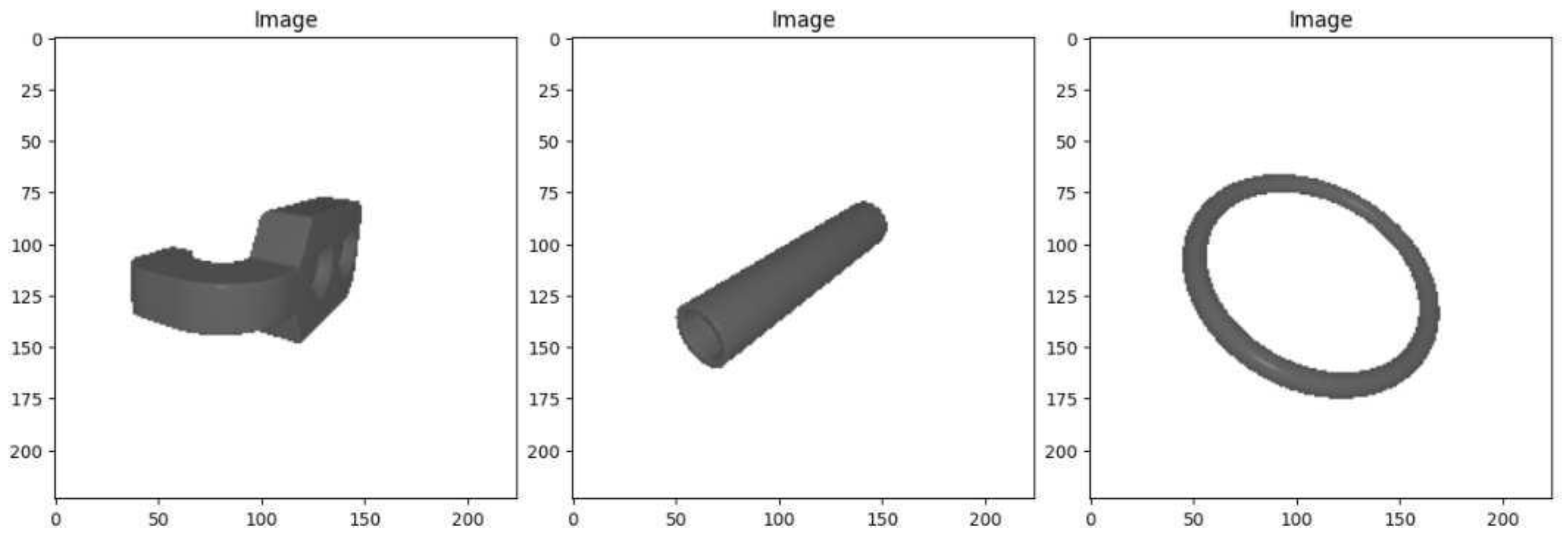
Figure 2.
Representation of the architecture for regressing poses from point clouds and images.
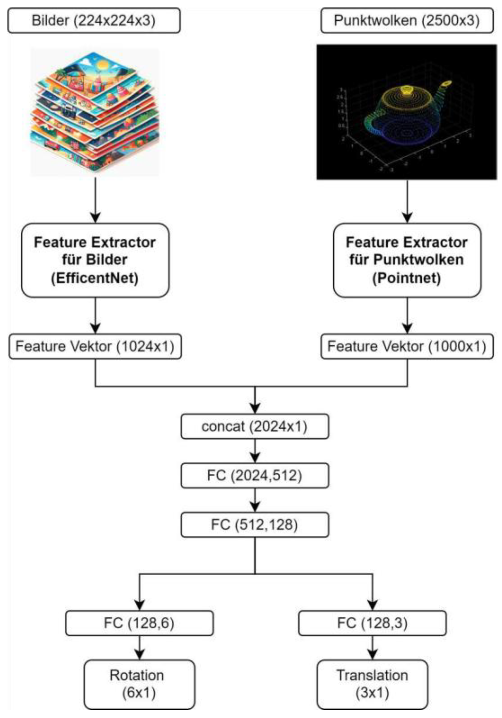
Figure 3.
Visualization of the Learning Curve for EfficientNet and PointNet.** As can be seen, the validation data reaches a final level of 0.2, which, on average, corresponds to a 20% deviation in the object radius.
Figure 3.
Visualization of the Learning Curve for EfficientNet and PointNet.** As can be seen, the validation data reaches a final level of 0.2, which, on average, corresponds to a 20% deviation in the object radius.
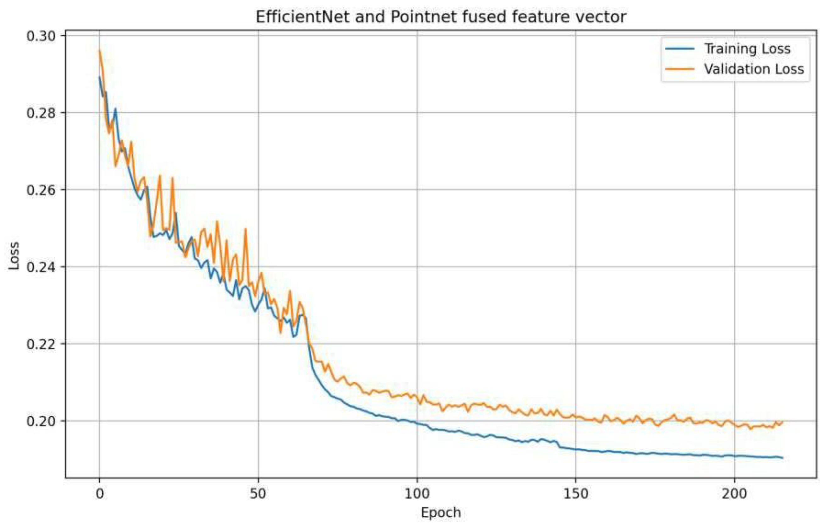
Figure 4.
Illustration of some estimations.
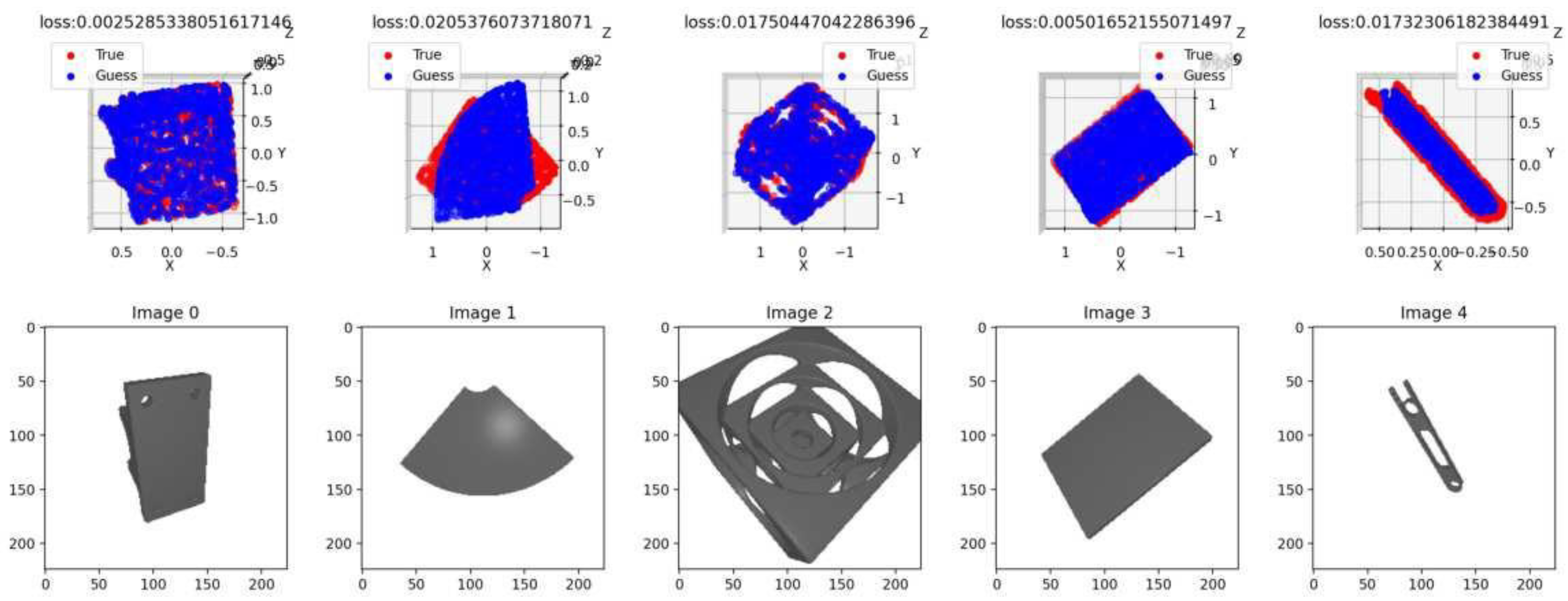
Figure 5.
Representation of the architecture of the U-Net modified with PointNet.
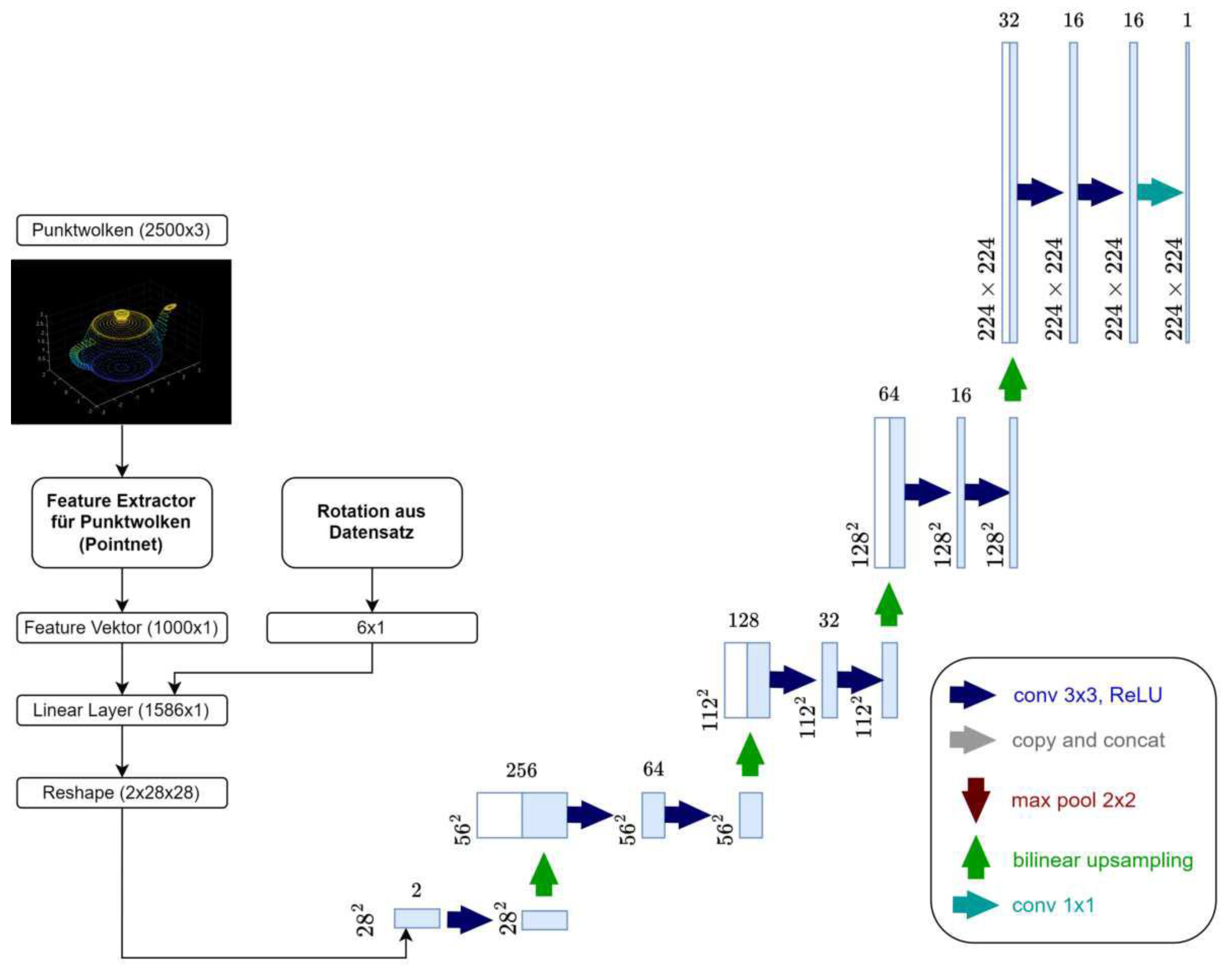
Figure 6.
Visualization of the test results of the trained model.
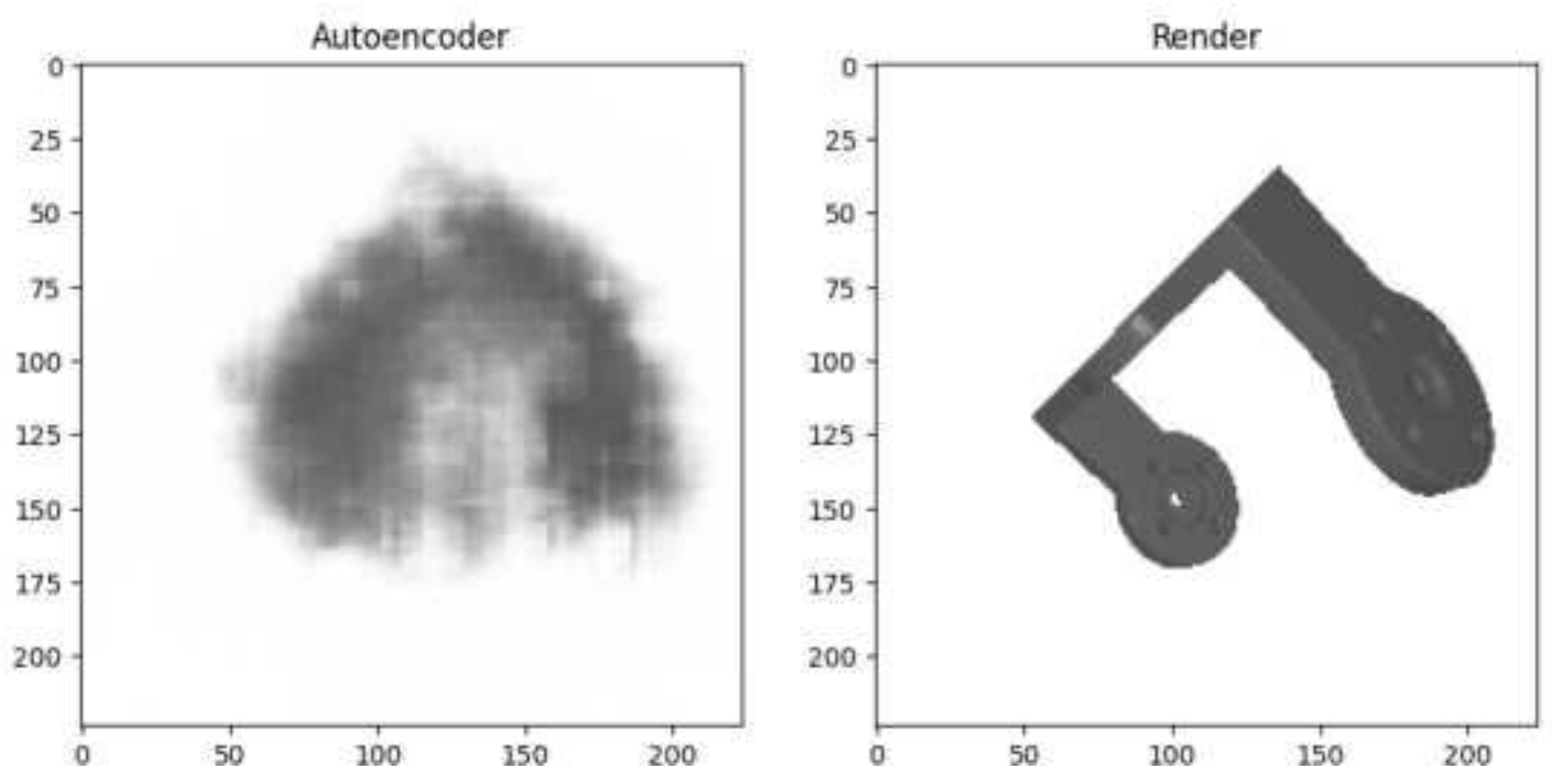
Figure 7.
Illustration of the Modified U-Net Autoencoder Architecture with PointNet Encoder and Regression using EfficientNet.
Figure 7.
Illustration of the Modified U-Net Autoencoder Architecture with PointNet Encoder and Regression using EfficientNet.
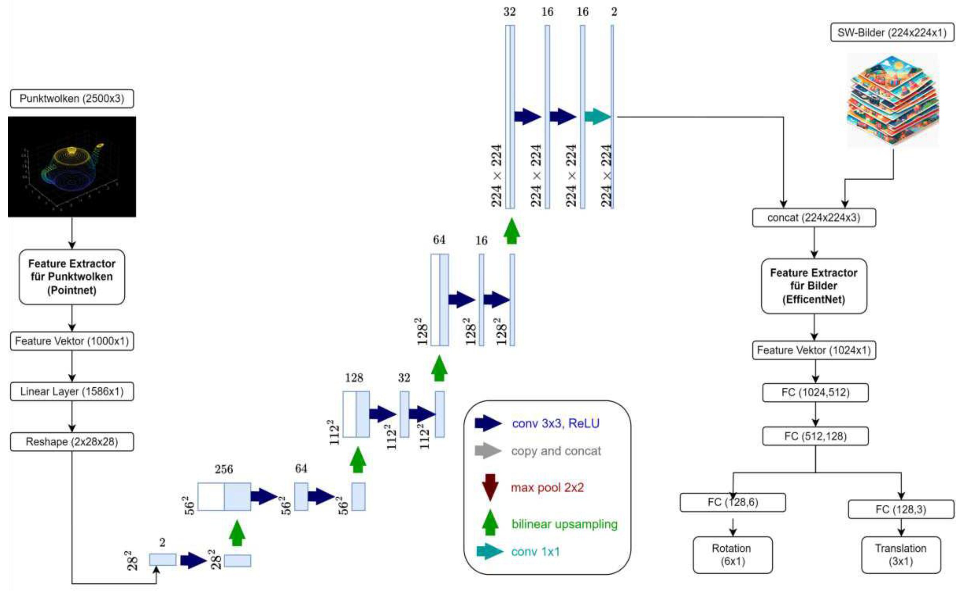
Figure 8.
Visualization of one of the two pseudo-images generated by the autoencoder. The target object was a triangular metal part.
Figure 8.
Visualization of one of the two pseudo-images generated by the autoencoder. The target object was a triangular metal part.
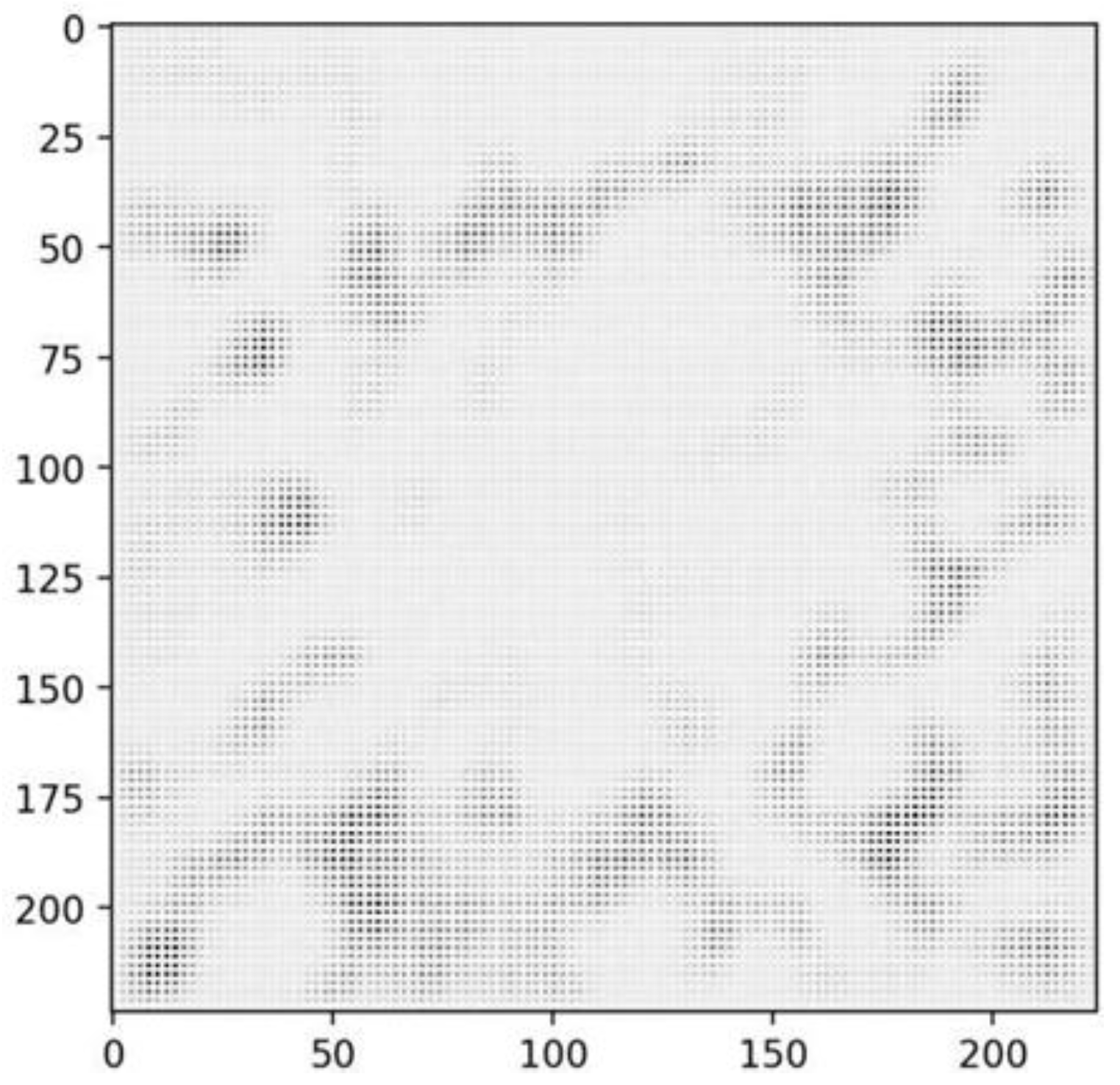
Figure 9.
Visualization of an image from the dataset. The target television is represented by its associated point cloud in red. The surrounding bounding sphere is depicted in green, and the central point is shown in blue.
Figure 9.
Visualization of an image from the dataset. The target television is represented by its associated point cloud in red. The surrounding bounding sphere is depicted in green, and the central point is shown in blue.
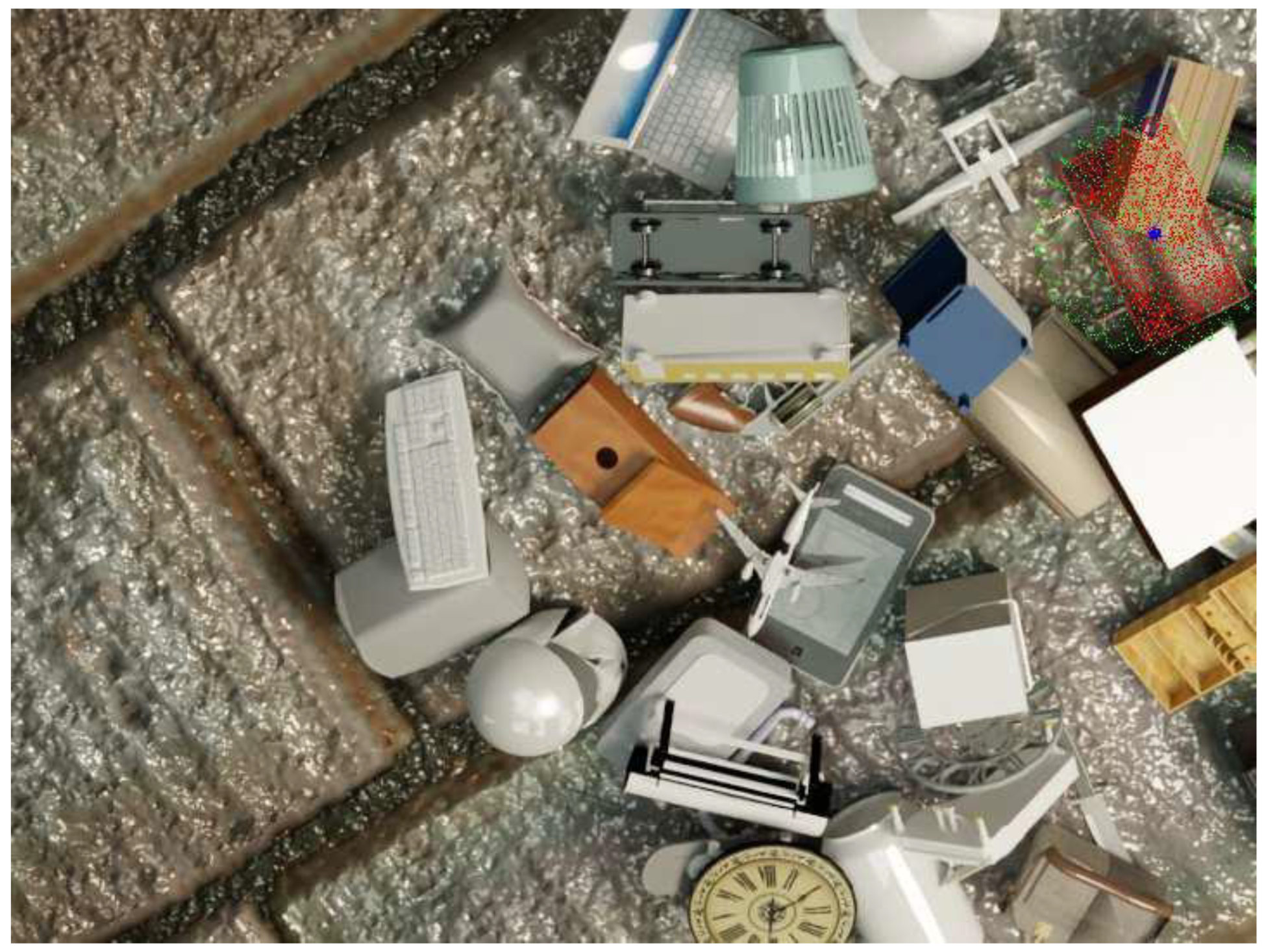
Figure 10.
Modified DETR architecture for the final system. The upper half depicts the original architecture from [41].
Figure 10.
Modified DETR architecture for the final system. The upper half depicts the original architecture from [41].
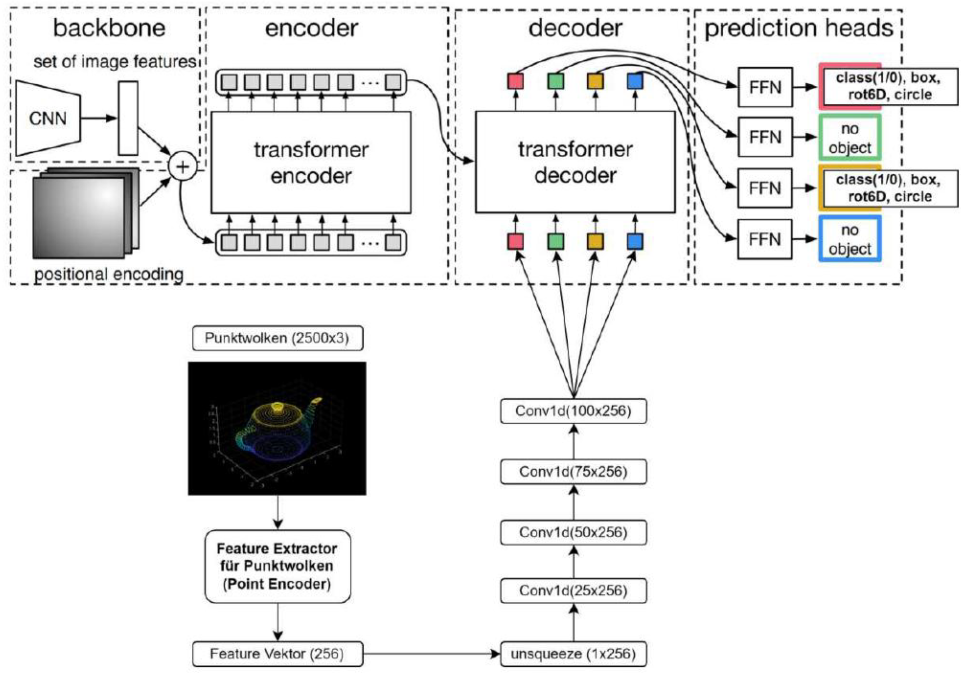
Figure 11.
The illustration of 2D bounding boxes highlights the presence of multiple rectangular objects, all detected by the network. The target object was the one marked with a green circle.
Figure 11.
The illustration of 2D bounding boxes highlights the presence of multiple rectangular objects, all detected by the network. The target object was the one marked with a green circle.
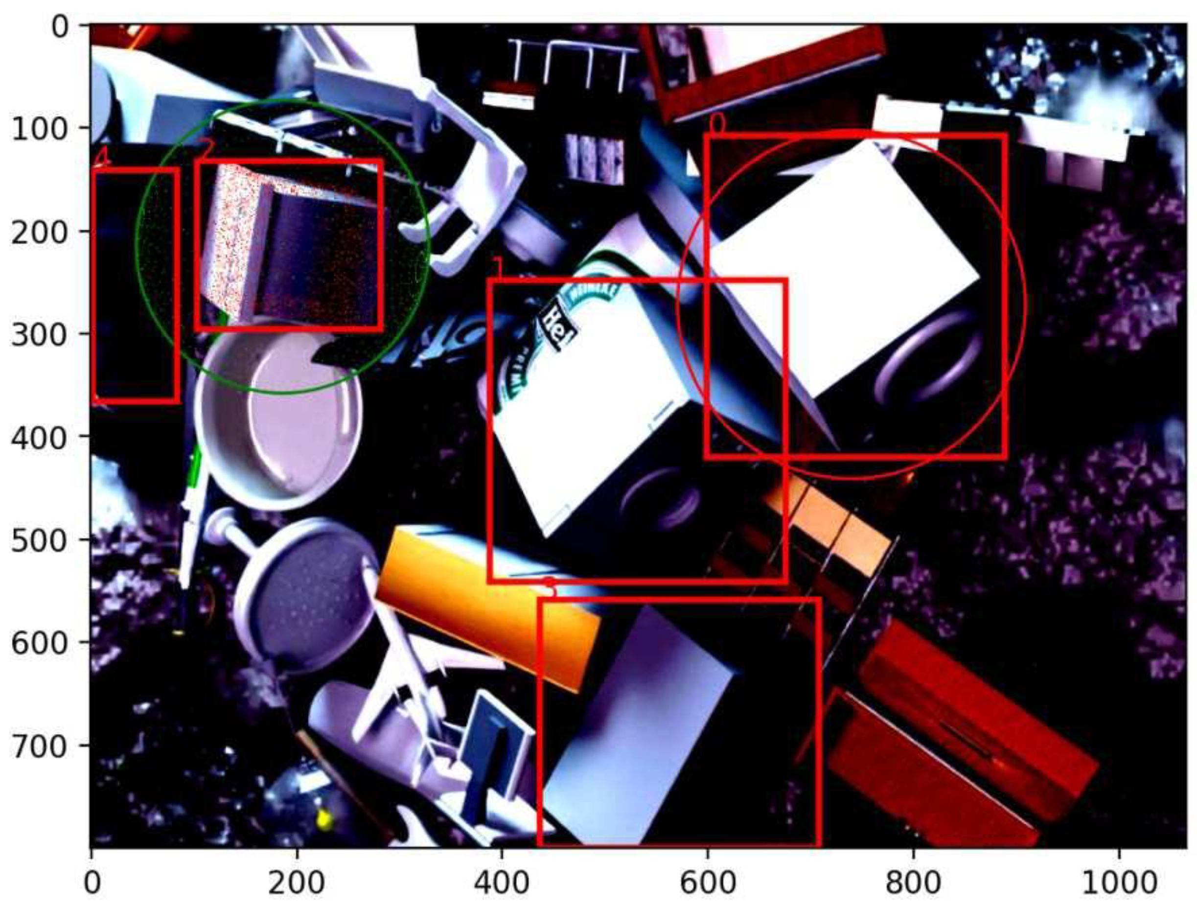
Figure 12.
The top section illustrates the network estimated position rotation compared to the actual object rotation. The bottom section shows the predicted bounding boxes, with bounding box 0 highlighted. Its corresponding circle (red for the estimate, green for the ground truth) and rotation are visible in the top section.
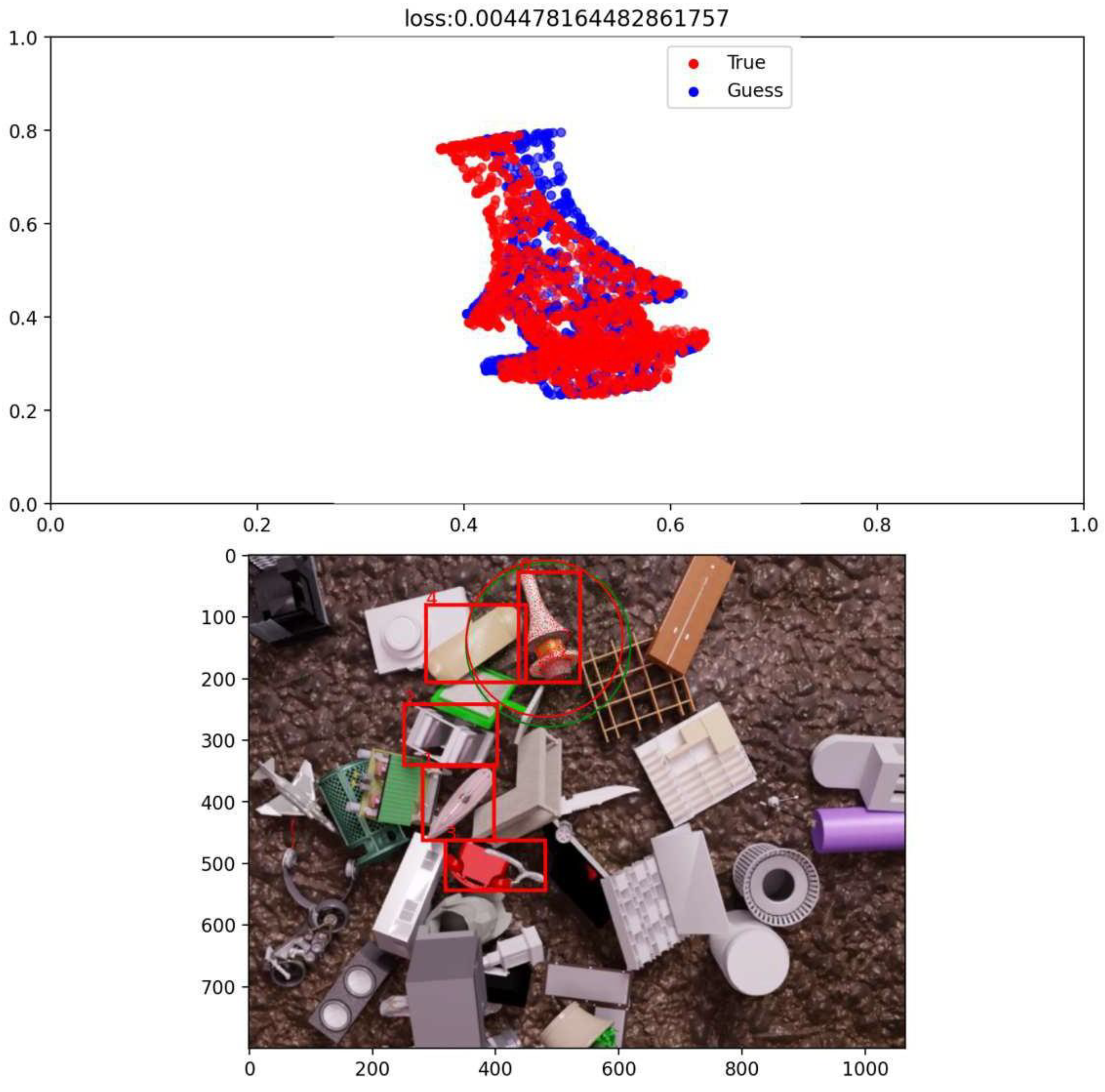
Figure 13.
Visualization of Pose Estimation in a Real Image.
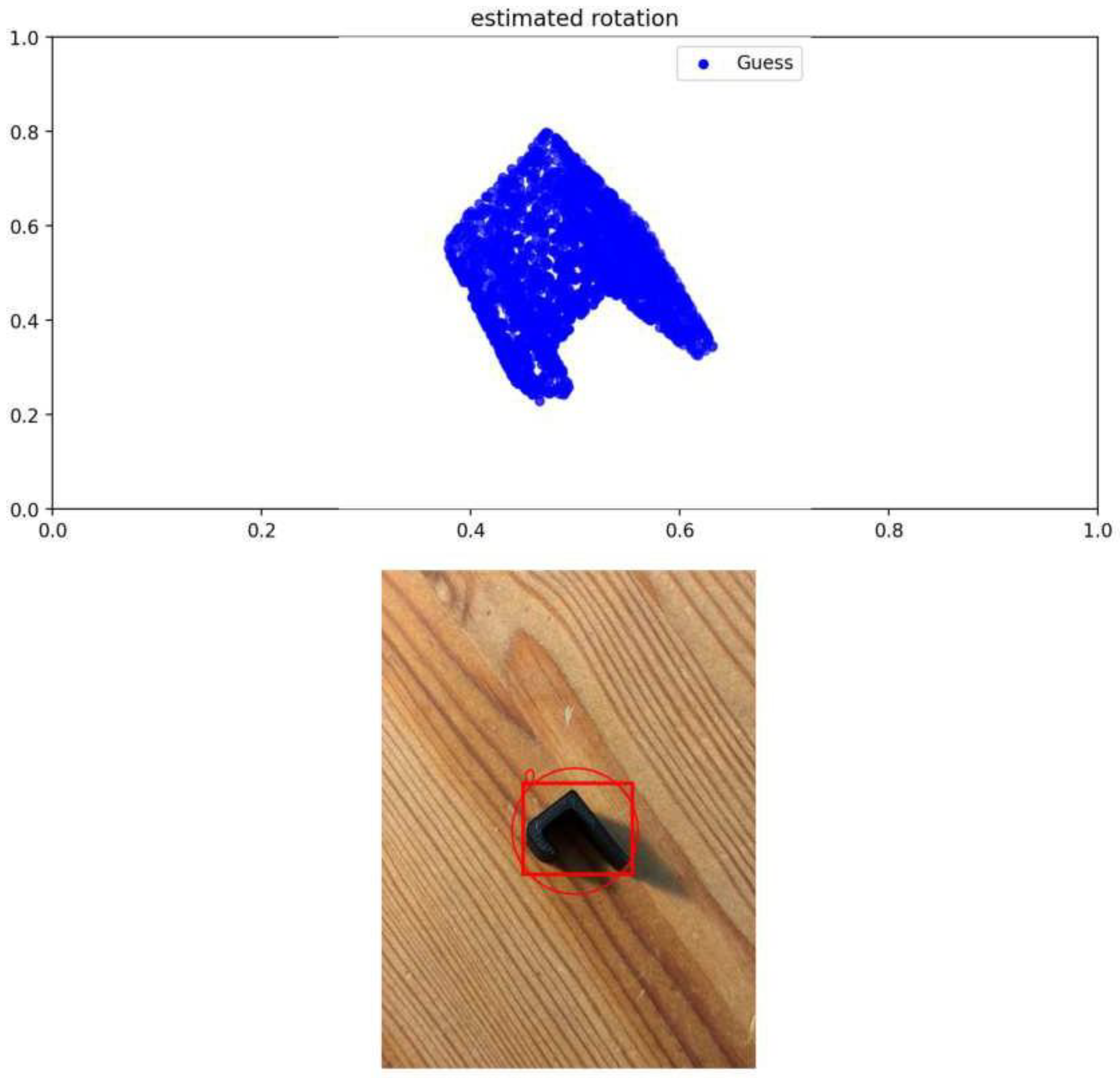

Table 1.
The L1 losses for the different approaches.
| PointNet Autoencoder | Point Embedding | ||
| Training | 0.19 | 0.205 | 0.175 |
| Validation | 0.2 | 0.22 | 0.182 |
Disclaimer/Publisher’s Note: The statements, opinions and data contained in all publications are solely those of the individual author(s) and contributor(s) and not of MDPI and/or the editor(s). MDPI and/or the editor(s) disclaim responsibility for any injury to people or property resulting from any ideas, methods, instructions or products referred to in the content. |
© 2025 by the authors. Licensee MDPI, Basel, Switzerland. This article is an open access article distributed under the terms and conditions of the Creative Commons Attribution (CC BY) license (http://creativecommons.org/licenses/by/4.0/).
Copyright: This open access article is published under a Creative Commons CC BY 4.0 license, which permit the free download, distribution, and reuse, provided that the author and preprint are cited in any reuse.


