
Submitted:
18 February 2025
Posted:
19 February 2025
You are already at the latest version
Abstract
In this study, a new compact "hot box" prototype (experimental cell) with a volume of 0.602 m³ has been designed, instrumented, and implemented to experimentally characterize the thermal conductivity of specimens measuring 25 cm x 25 cm, with the thickness of the specimen varying up to a maximum of 10 cm. The prototype features a novel design aimed at enhancing flexibility and speed in changing specimens, thereby reducing downtime when testing different materials. It requires minimal space and incurs low development and maintenance costs. To validate the prototype's functionality for measuring thermal conductivity, an oak wood specimen with a thickness of 3.81 cm was experimentally tested. The results indicate that the control system maintains key parameters under steady-state conditions for a significant duration. The thermal conductivity obtained for the oak wood specimen is 0.1695 W/m-1·K-1, with an expanded uncertainty of 0.0183 W/m-1·K-1 for a 95% confidence interval.
Keywords:
hot box method
; thermal conductivity
; heat flux
; surface temperature
; steady state
; oak specimen
1. Introduction
In the energy transition, buildings are considered a low-carbon emission energy system. In the current context, residential and commercial buildings are responsible for consuming one-third of the electricity produced globally and generating 17% of emissions [1]. Based on these characteristics, buildings represent a key target for improving energy efficiency, environmental sustainability, and financial viability. Therefore, buildings are undergoing an adaptation process to address the urgent need for efficient and sustainable construction systems, both environmentally and financially. This necessity has driven the construction industry, research institutes, and universities to explore alternatives for optimizing the energy performance of buildings in an environmentally friendly and efficient manner.
The materials used in the building envelope and interior are directly correlated with energy efficiency, indoor thermal comfort, lifecycle performance, and financial balance. Thus, the mechanical, thermal, and acoustic properties of materials play a key role in developing construction solutions. In this regard, measuring these parameters ensures a better understanding of how materials influence the energy efficiency of construction systems. In the current scenario, the integration of new materials derived from agricultural [2,3,4]and industrial [5] waste for manufacturing insulating panels used in building envelopes and interiors is becoming increasingly popular. These new insulating panels are highly diverse, as they originate from local production byproducts. Consequently, there is an urgent need to design alternative methods for measuring thermal conductivity in a more flexible, accessible, and cost-effective manner than currently available methods [6].
Thermal conductivity is a fundamental parameter for calculating the thermal transmittance of construction materials, thus providing a benchmark that helps classify the insulation level of a material. Currently, different instrumental methods exist for measuring thermal conductivity, which can be classified into two main categories: steady-state and transient measurement techniques [7]. In general, commercial equipment used to measure thermal conductivity has prohibitive costs, limiting or preventing its availability in developing countries.
In the case of the hot box method, ISO 8990:1994 [8] and ASTM-C518 [9] standards focus on characterizing thermal transmittance using the hot box methodology, which is classified into two types based on experimental techniques: guarded and calibrated hot boxes. In both cases, the specimen acts as a separator between a hot and a cold chamber, with a minimum dimension of 1m × 1m. As a result, significant laboratory space, high maintenance costs, structural complexity of the hot chamber, long testing durations, and high energy consumption are required [10]. In literature, extensive efforts are being made to develop alternative methodologies for determining thermal conductivity, as evidenced by the following studies [11,12,13,14,15].
In this study, we propose a novel experimental cell prototype for characterizing thermal conductivity based on the hot box methodology. First, the experimental cell prototype was designed. Then, a control system was developed to regulate the thermal load, generating a temperature gradient between the chambers. Finally, the prototype was instrumented with the necessary sensors to compute the thermal conductivity of any specimen. The new experimental cell was built with dimensions of 81 cm (height) × 61 cm (width) × 122 cm (length), resulting in a physical volume of 0.602 m³. It allows testing specimens with a fixed area of 25 cm × 25 cm, with a variable thickness of up to 10 cm. To validate the experimental cell, a specimen made of oak wood—whose thermal conductivity has been widely tested and confirmed by various laboratories—was used.
This article is structured as follows: the first section corresponds to the introduction; the second section presents the materials and methods used, including the box architecture, instrumentation, and control system design. Section three focuses on analyzing the obtained results
2. Materials and Methods
The experimental cell was developed in the Sustainable Construction Solutions Laboratory with the primary purpose of characterizing the thermal conductivity of insulating panels made from both traditional materials and new materials derived from agricultural or industrial waste. Figure 1 presents a schematic of the experimental cell, which was designed considering several recommendations from the ISO-8990:1994 standards. It is important to note that the constructed prototype falls outside the full scope of the standard, which specifies a minimum specimen size of 1 m × 1 m. The proposed flexible design helps address laboratory space constraints, maintenance and operational costs, and improves the speed of test preparation.
2.1. Experimental Cell Architecture
The experimental cell was constructed using a layered format:
- The outer layer consists of plywood with a thickness of 1.5 cm, forming the external enclosure.
- The intermediate layer is made of expanded polystyrene with a thickness of 20 cm, a density of 20 kg/m³, and a thermal conductivity of 0.0358 W/m·K.
- The inner layer consists of hardboard sheets with a thickness of 1 cm.
The external enclosure is fully sealed with lateral and top covers that fit together using embedded slots. The geometric dimensions of the cell prototype are listed in Table 1.
The prototype consists of two chambers, identified as the hot chamber and the cold chamber, whose dimensions are provided in Table 1. Both chambers are separated by a specimen holder, which is built with an outer layer of 1.5 cm plywood and an interior filled with expanded polystyrene to enhance insulation (Figure 1). The specimen holder serves two functions:
- Separating the airflow between the hot and cold chambers, ensuring both physical and thermal division.
- To hold the specimen, ensuring direct contact between the circulating air in both chambers and the specimen surfaces (Figure 1).
The specimen holder consists of two separate symmetrical pieces: one acting as the base and the other as the closure. The test specimen is placed in the center of the holder using machine slots in both the base and closure pieces. The holder was designed to accommodate panel specimens with dimensions of 25 cm × 25 cm × Z cm, where Z can vary up to a maximum thickness of 10 cm.
As shown in Figure 1, the specimen holder is integrated into the experimental cell enclosure through lateral sliding slots. This embedded coupling ensures a tighter seal and minimizes heat losses between the chambers, in accordance with the construction recommendations of the standard [8]. To install a specimen in the holder, the base piece is first assembled within the enclosure. Then, the specimen is placed on the slot of the base piece. To compensate for possible sealing irregularities between the holder and the specimen, the lateral edges are covered with a thin elastomeric foam layer (3–5 mm thick), preventing potential air leaks between chambers and thermal bridging. Finally, the closure piece is inserted into the enclosure to fully separate the chambers.
During the commissioning process, various insulation thicknesses for the intermediate layer were tested. The optimal thickness was determined using thermographic techniques, identifying thermal bridges and temperature distribution through infrared imaging, as shown in Figure 2. Additionally, the experimental cell was equipped with four wheels to allow easy mobility.
2.2. Instrumentation and Control
Thermal conductivity is determined from experimental measurements obtained under conditions close to steady-state operation. This approach ensures a uniform temperature distribution on the specimen surfaces over a period. The temperature gradient and uniformity of temperature distribution are achieved by creating artificial atmospheres within the hot and cold chambers.
In the hot chamber, the internal atmosphere is established by supplying a thermal load using an electric resistance array to heat the air. To ensure homogeneous airflow, an axial fan is positioned near the thermal resistance to force air circulation by convection (Table 3). The heating elements are helical resistances, each with a resistance of approximately 96 Ω and a power rating of 100–125 W. The electrical power supply and fan speed are controlled by adjusting the supply voltage using a dimmer (Table 2).
Inside the hot chamber, at 32cm from the specimen and 22 cm from the fan, a 0.5 cm plywood vertical shield is installed to protect the specimen from internal radiation effects generated by the resistance and direct airflow. Additionally, the entire inner perimeter of the hot chamber is lined with a hardboard, a low-emissivity material, which helps mitigate radiation effects and prevents the expanded polystyrene layer from coming into direct contact with the thermal resistance.
To maintain steady-state operating conditions, the hot chamber requires a control system that adjusts the thermal load based on internal air temperature. Since the prototype’s hot chamber exhibits high thermal inertia, a control strategy was needed to optimize response time for each test. For this reason, a lead compensator with integral action was implemented to reduce steady-state error without significantly affecting settling time. A PWM-based thermal regulation system, using an array of electric resistances, was employed to control heat flux within the hot chamber, maintaining near-steady-state conditions.
In the cold chamber, the internal atmosphere is directly influenced by laboratory conditions, as it is open to the surrounding environment. Consequently, the air temperature is affected by the ambient conditions. To enhance control over the laboratory atmosphere, a dedicated space of 215 cm (width) × 300 cm (length) × 275 cm (height) was allocated, equipped with an air conditioning system dedicated exclusively to the laboratory.
2.3. Measurement and Data Acquisition
Process monitoring is performed using surface temperature sensors and heat flux thermopile sensors, which are fixed to the specimen surfaces. The sensors are connected to a LabJack T7-Pro data acquisition system, whose specifications are detailed in Table 3.
To measure surface temperature on the specimen in the hot chamber, five Type T surface thermocouples were used, distributed as follows:
- One thermocouple at the center of the specimen.
- Four thermocouples 15 cm from the center, positioned at the north, south, east, and west coordinates (Figure 3).
This arrangement allows temperature distribution uniformity to be analyzed. The heat flux density is measured using two PHFS-01e thermopile-type heat flux sensors, mounted on the specimen surface. Figure 3 illustrates the sensor distribution:
- One heat flux sensor is placed at the center of the specimen.
- Another is located 15 cm south of the center.
- The specifications of these sensors are summarized in Table 2.
- On the cold chamber side, two Type T surface thermocouples are fixed on the specimen: one at the center and another 15 cm north of the center.
To manage thermal load control, monitor, and store measured variables, a custom interface was developed using Python. Data acquisition was performed at a sampling rate of one (1) second, and each test generated a data file containing all measured variables. Data processing and analysis were conducted using MATLAB 2022b.
3. Thermal Conductivity
Thermal conductivity is determined by using Fourier’s principle for heat transfer through a material, assuming a unidirectional heat transmission, steady-state operation, and that the specimen’s properties remain unchanged along the direction of heat flow.
The thermal conductivity model (λ) relates the heat flux density (), the specimen thickness dx, the average temperature of the specimen’s hot surface ( ), and the average temperature of the specimen’s cold surface ( ).
To assess the reliability of the experiment, an uncertainty analysis was performed following the recommendations established in the Guide to the Expression of Uncertainty in Measurement (GUM) [16]. The propagation of uncertainty through the variables associated with thermal conductivity is estimated using the Taylor series expansion:
The combined uncertainty (ux) is calculated by integrating Type A and Type B uncertainties for each variable that contributes to λ.
Type A uncertainty is estimated based on the repeatability of measurements using . Type B uncertainty is associated with the manufacturing specifications of the measuring instruments. The expanded uncertainty inherent to the thermal conductivity for a 95% confidence level is then calculated accordingly.
4. Results and Discussion
In this study, a new experimental cell prototype with a physical volume of 0.602 m³ was designed to measure the thermal conductivity of a specimen with a thickness of less than 10 cm and a fixed area of 25 cm × 25 cm using the hot-box technique. The prototype was equipped with a thermal regulator to adjust the internal atmosphere of the hot chamber, generating a temperature difference across the specimen with the cold chamber. The atmosphere inside the cold chamber depends on the environmental conditions of the laboratory, which are controlled using a dedicated air conditioning system.
To validate the prototype’s operation, an experimental test was conducted with an Oak-based specimen with an area of 25 cm × 25 cm and a thickness of 3.81 cm. The Oak sample was selected because it corresponds to a well-known construction material with widely studied thermal properties. This selection facilitates the comparison of the experimental thermal conductivity value obtained with the new prototype against reference values from laboratories and studies reported in the literature.
The experimental process carried out with the prototype is illustrated in Figure 4. The total experiment duration was 1.5 hours, corresponding to 5,400 readings. It is important to note that experimental measurements were recorded only after the hot chamber reached the target setpoint temperature of 70 °C established for this study. Figure 5a shows the temperature behavior captured by the sensors positioned at the center, south, west, north, and east of the Oak specimen throughout the entire test (1.5 h). It can be observed that the temperatures exhibit minimal fluctuations and remain close to the setpoint value (70 °C). The ambient laboratory temperature and the temperatures measured on the cold surface of the specimen are shown in Figure 5b. The laboratory temperature remains approximately constant at 21 °C, while the temperatures on the cold surface of the specimen display smooth lines without disturbances, with a central value close to 38 °C.
The measurements obtained from the heat flux sensors positioned at the center and south coordinate of the Oak specimen during the experiment exhibit rapid short-spectrum oscillations (Figure 5c). This behavior has been reported in other studies [10,17], suggesting that it could be associated with transient phenomena caused by rapid fluctuations in the temperature differential due to small changes in the internal atmosphere of the hot chamber.
The thermal conductivity (Equation (1)) obtained from the average values of the main parameters recorded in each reading is shown in Figure 5d. Initially, the trend of the curve continuously decreases until it converges to an approximately constant value (Figure 5d). This behavior is expected according to the ISO-9869-1:2014 standard [18] and has been observed in theoretical studies by other authors [10,13].
The total thermal conductivity was evaluated using the experimental measurements recorded under steady-state conditions during the test, totaling 2,700 readings over 45 minutes. The average values for each reading of the main parameters associated with thermal conductivity are presented in Figure 6a. All average values of the hot and cold surface temperatures of the specimen remain close to constant conditions. The heat flux shows short oscillations with a central value of 130 W・m⁻². The temperature difference between the hot and cold surfaces of the Oak specimen remains approximately 30 °C. The test characteristics are detailed in Table 4. In Figure 6b, it can be observed that the thermal conductivity calculated using the average values of the specimen under steady-state conditions remains within a narrow control range, with a difference between the minimum and maximum value of 0.0580 W・m⁻¹・K⁻¹.
The total thermal conductivity value obtained corresponds to 0.1695 W・m⁻¹・K⁻¹, with an associated uncertainty in the range of ±0.0183 W・m⁻¹・K⁻¹ for a 95% confidence interval. This thermal conductivity value is consistent with values reported by other laboratories and commercial equipment for an Oak specimen [19,20,21]. The average values of the main parameters for the specimen under steady-state conditions and the total thermal conductivity are summarized in Table 4.
5. Conclusions
In this study, a new experimental cell prototype with a volume of 0.602 m³ was developed to characterize the thermal conductivity of specimens with a fixed area of 25 cm × 25 cm and the possibility of varying the thickness up to 10 cm. To validate the prototype’s operability, a 3.81 cm-thick oak wood specimen was tested.
The main findings are summarized as follows:
- The PWM-based thermal regulator, designed to adjust the internal atmosphere of the hot chamber by supplying a heat flux, performed well, maintaining an air temperature close to steady-state conditions.
- The temperature difference between the hot and cold surfaces of the specimen remained close to 30°C in the transient regime identified during the experimental test.
- A thermal conductivity of 0.1695 W·m⁻¹·K⁻¹ was obtained, with an expanded uncertainty of ±0.0183 W·m⁻¹·K⁻¹ at a 95% confidence interval. Therefore, the relative uncertainty of the experiment corresponds to 10.78% of the thermal conductivity. This thermal conductivity value falls within the reference range reported by other laboratories and commercial equipment for an oak wood specimen.
The developed prototype could contribute to obtaining preliminary thermal conductivity values, enhancing the flexibility and speed of tests with different specimens, while occupying less laboratory space and maintaining a non-prohibitive cost. Future studies aim to test various specimens made from agricultural waste materials.
Author Contributions
Conceptualization, investigation and methodology, F.R., N.G. and Y.G.; software, validation, formal analysis, F.R. and N.G.; resources, D.V. and M.M..; data curation, D.V. and M.M.; writing—original draft preparation, D.V. and M.M.; writing—review and editing, F.R. and N.G.; visualization, D.V. and M.M.; supervision and project administration, Y.G.; funding acquisition, F.R. and Y.G.
Funding
This research was funded by National Fund for Innovation and Scientific and Technological Development (FONDOCyT), a program of the Ministry of Higher Education, Science, and Technology (MESCYT), Project codes: AgroAislantes 2020-2021-3B1-085, WasteBlocks 2022-3A11-153 and Evaluation of the energy performance of a low-power cooling production system using organic refrigerants assisted by photovoltaic solar energy 2023-1-3C2-0697.
Conflicts of Interest
The authors declare no conflicts of interest.
References
- “World Energy Outlook 2023 – Analysis - IEA.” Accessed: Feb. 05, 2025. [Online]. Available: https://www.iea.org/reports/world-energy-outlook-2023.
- Z. Balador, M. Gjerde, N. Isaacs, and M. Imani, “Thermal and Acoustic Building Insulations from Agricultural Wastes,” Handbook of Ecomaterials, pp. 1–20, 2018. [CrossRef]
- K. Selvaranjan et al., “Thermal and environmental impact analysis of rice husk ash-based mortar as insulating wall plaster,” Constr Build Mater, vol. 283, p. 122744, May 2021. [CrossRef]
- S. Mehrzad, E. Taban, P. Soltani, S. E. Samaei, and A. Khavanin, “Sugarcane bagasse waste fibers as novel thermal insulation and sound-absorbing materials for application in sustainable buildings,” Build Environ, vol. 211, p. 108753, Mar. 2022. [CrossRef]
- P. Ricciardi, E. Belloni, F. Merli, and C. Buratti, “Sustainable Panels Made with Industrial and Agricultural Waste: Thermal and Environmental Critical Analysis of the Experimental Results,” Applied Sciences 2021, Vol. 11, Page 494, vol. 11, no. 2, p. 494, Jan. 2021. [CrossRef]
- M. Ghobadi and S. M. E. Sepasgozar, “Circular economy strategies in modern timber construction as a potential response to climate change,” Journal of Building Engineering, vol. 77, p. 107229, Oct. 2023. [CrossRef]
- Palacios, L. Cong, M. E. Navarro, Y. Ding, and C. Barreneche, “Thermal conductivity measurement techniques for characterizing thermal energy storage materials – A review,” Renewable and Sustainable Energy Reviews, vol. 108, pp. 32–52, Jul. 2019. [CrossRef]
- “ISO 8990:1994 - Thermal insulation — Determination of steady-state thermal transmission properties — Calibrated and guarded hot box.” Accessed: Feb. 05, 2025. [Online]. Available: https://www.iso.org/standard/16519.html.
- “Standard Test Method for Steady-State Thermal Transmission Properties by Means of the Heat Flow Meter Apparatus, ASTM C518-21 | Building America Solution Center.” Accessed: Feb. 05, 2025. [Online]. Available: https://basc.pnnl.gov/library/standard-test-method-steady-state-thermal-transmission-properties-means-heat-flow-meter.
- Barbaresi, M. Bovo, E. Santolini, L. Barbaresi, D. Torreggiani, and P. Tassinari, “Development of a low-cost movable hot box for a preliminary definition of the thermal conductance of building envelopes,” Build Environ, vol. 180, p. 107034, Aug. 2020. [CrossRef]
- Y. G. Frómeta, F. R. Rivera, V. G. Holguín, and J. Cuadrado, “Experimental Investigation of Thermal Conductivity from Insulation Based on Rice Hulks: Guarded and Calibrated Hot Box Method,” Materials Science Forum, vol. 1046, pp. 71–76, 2021. [CrossRef]
- E. Roque, R. Vicente, R. M. S. F. Almeida, J. Mendes da Silva, and A. Vaz Ferreira, “Thermal characterisation of traditional wall solution of built heritage using the simple hot box-heat flow meter method: In situ measurements and numerical simulation,” Appl Therm Eng, vol. 169, p. 114935, Mar. 2020. [CrossRef]
- R. Ricciu, A. Galatioto, L. A. Besalduch, G. Desogus, and L. Di Pilla, “Building Wall Heat Capacity Measurement Through Flux Sensors,” [Journal of Sustainable Development of Energy, Water and Environment Systems], vol. [7], no. [1], p. [44]-[56], Mar. 2019. [CrossRef]
- Gounni et al., “Thermal and economic evaluation of new insulation materials for building envelope based on textile waste,” Appl Therm Eng, vol. 149, pp. 475–483, Feb. 2019. [CrossRef]
- Alhawari, A. Alhawari, and P. Mukhopadhyaya, “Construction and Calibration of a Unique Hot Box Apparatus,” Energies 2022, Vol. 15, Page 4677, vol. 15, no. 13, p. 4677, Jun. 2022. [CrossRef]
- JCGM, “Evaluation of measurement data-Guide to the expression of uncertainty in measurement Évaluation des données de mesure-Guide pour l’expression de l’incertitude de mesure,” 2008, Accessed: Feb. 05, 2025. [Online]. Available: www.bipm.org.
- Buratti, E. Belloni, L. Lunghi, A. Borri, G. Castori, and M. Corradi, “Mechanical characterization and thermal conductivity measurements using of a new ‘small hot-box’ apparatus: innovative insulating reinforced coatings analysis,” Journal of Building Engineering, vol. 7, pp. 63–70, Sep. 2016. [CrossRef]
- “ISO 9869-1:2014 - Thermal insulation — Building elements — In-situ measurement of thermal resistance and thermal transmittance — Part 1: Heat flow meter method.” Accessed: Feb. 05, 2025. [Online]. Available: https://www.iso.org/standard/59697.html.
- J. Martínez et al., “Caracterización Térmica y Mecánica de la Madera de Roble,” Revista Técnica “energía,” vol. 16, no. 1, pp. 88–96, Jul. 2019. [CrossRef]
- H. Ş. Kol, “The Transverse Thermal Conductivity Coefficients of Some Hardwood Species Grown in Turkey,” For Prod J, vol. 59, no. 10, pp. 58–63, Oct. 2009. [CrossRef]
- F. Peron, P. Bison, M. De Bei, and P. Romagnoni, “Thermal properties of wood: measurements by transient plane source method in dry and wet conditions,” J Phys Conf Ser, vol. 1599, no. 1, p. 012050, Aug. 2020. [CrossRef]
Figure 1.
Illustrative diagram of the experimental cell.
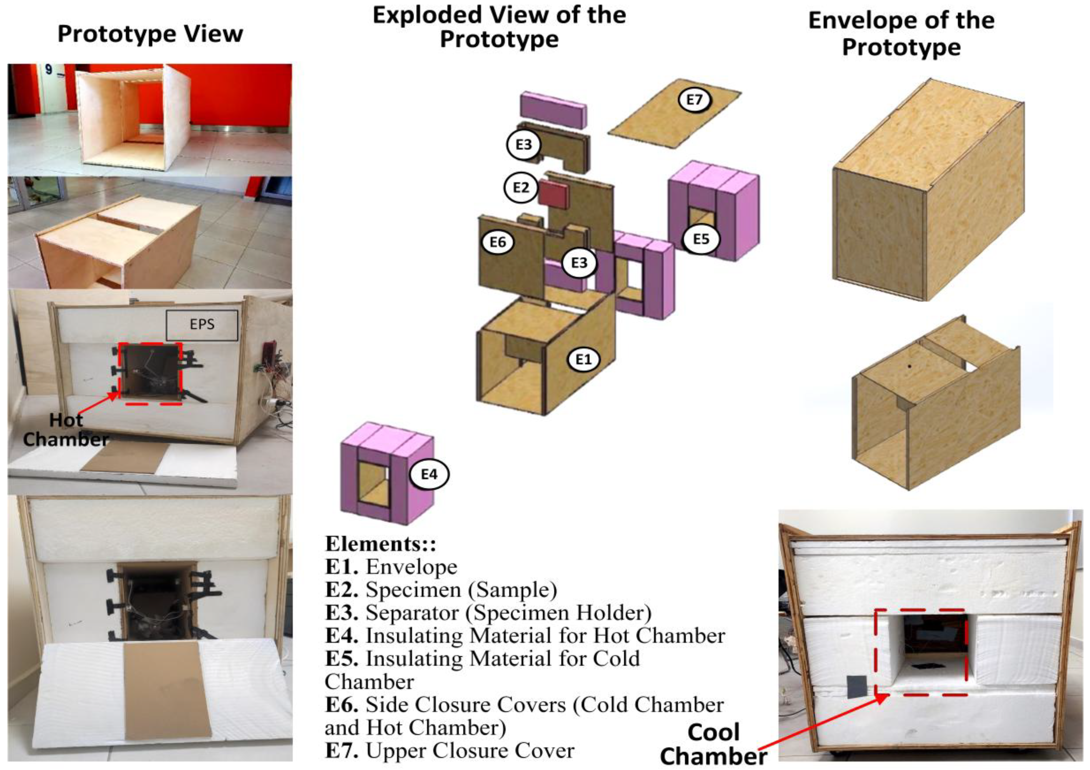
Figure 2.
Thermographic images of the outer contour of the experimental cell during a test. (a) Front, (b) Side, (c) Top.
Figure 2.
Thermographic images of the outer contour of the experimental cell during a test. (a) Front, (b) Side, (c) Top.
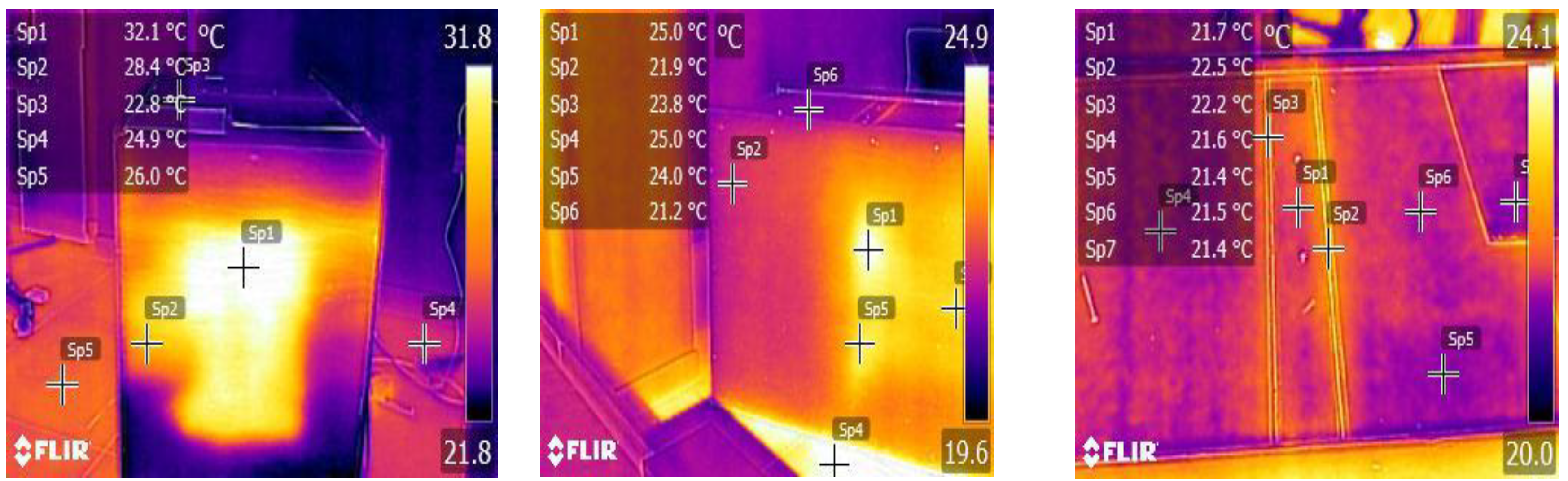
Figure 3.
Distribution of sensors on the surface of the specimen.
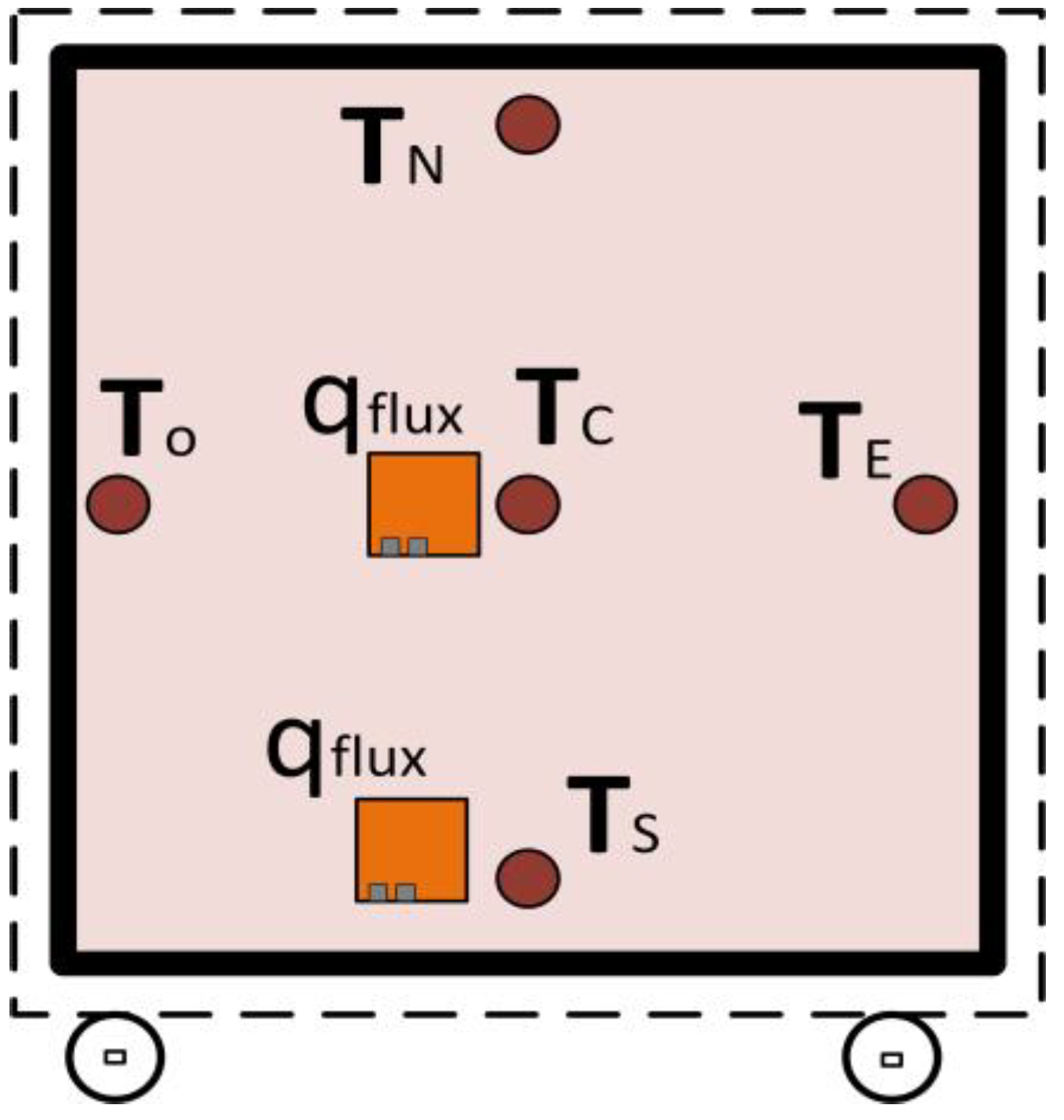
Figure 4.
Process flow for performing specimen testing.
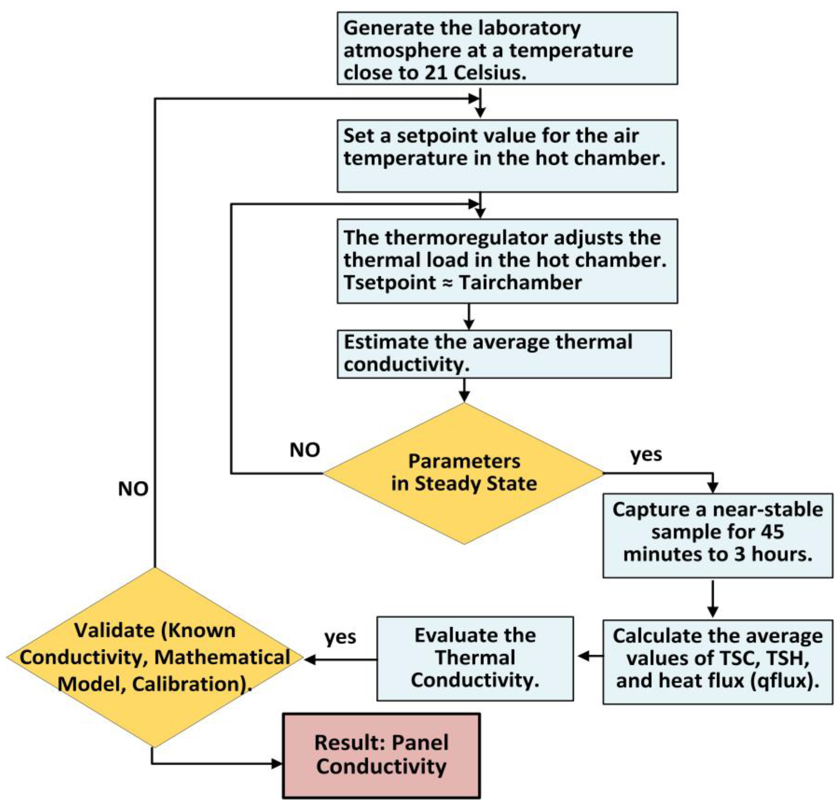
Figure 5.
Trend of the main parameters during the test to estimate the thermal conductivity of the Oak specimen. (a) Temperature profile on the Oak specimen in the hot chamber, (where THCenter THsouth, THWest, THNorth, THEast, represent the sensor measurement at the center, south, west, north, east of the Oak specimen) (b) Temperature behavior on the surface of the Oak specimen in the cold chamber (TCoolCenter, TCoolCenter) and the ambient temperature (TAmb) in the laboratory during the test, (c) Evolution of the heat flow obtained with the sensors fixed at the center and south coordinate of the surface of the Oak specimen, (d) Thermal conductivity of the Oak specimen for each measurement captured in the test.
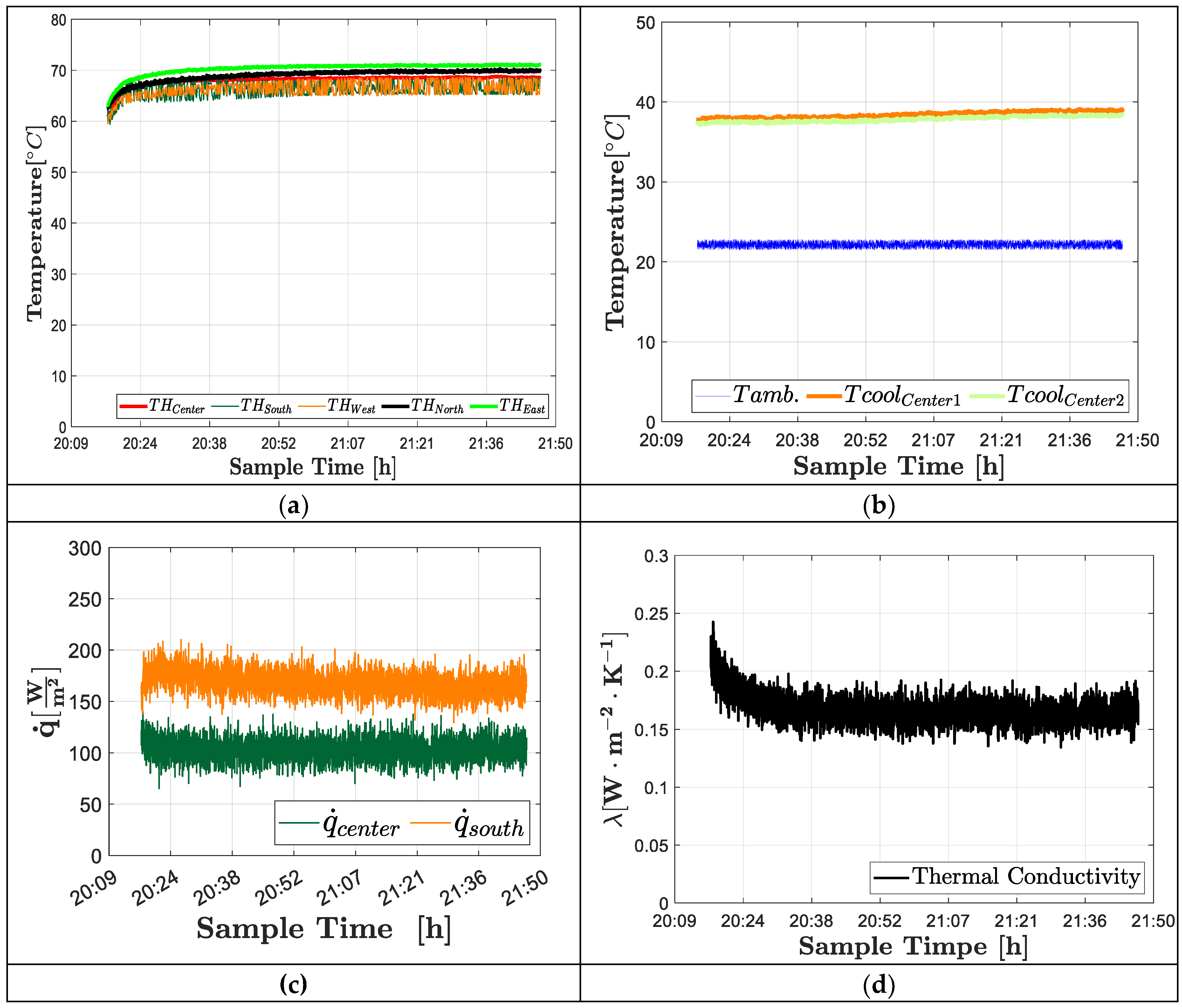
Figure 6.
Steady-state sample for a period of 45 minutes. (a) Average value of the parameters that define the thermal conductivity, where ¯ TSHot and TSCool correspond to the average temperature of the hot and cold surfaces of the Oak specimen, heat flux density on the hot surface of the specimen, (b) Average thermal conductivity.
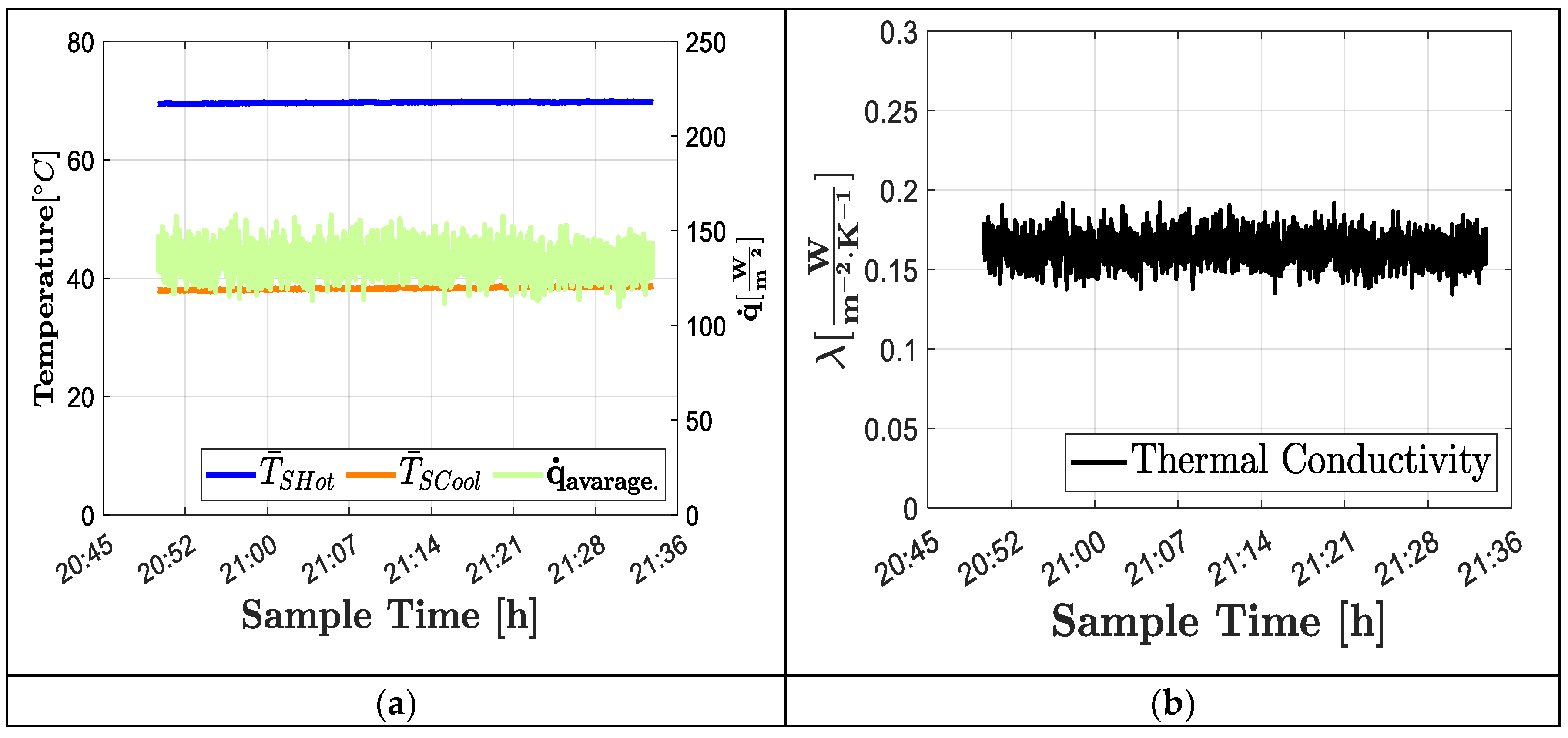

Table 1.
Geometry of the experimental cell.
| Parameters | Dimensions (H x W x L) |
|---|---|
| Experimental cell | 81cm x 61cm x 122cm |
| Hot chamber | 33cm x 20cm x 61cm |
| Cold chamber | 26cm x 20cm x 44cm |
| Specimen carrier | 75cm x 60cm x 10cm |
Table 2.
Characteristics of measuring instruments.
| Variables | Sensor | Range | Precision |
|---|---|---|---|
| Surface temperature | Type T | [-30 250] °C | ±0.5 C |
| Heat flow | Thermopile | [-150 150] kW/m^2 | 7.7 mV/(W/cm^2) |
Table 3.
Equipment used in the experimental cell.
| Equipment | Model | Characteristics |
|---|---|---|
| Datalogger | LabJack T7-Pro | 14 analog inputs, Communication: USB, Ethernet802.11b/g WiFi speed:16 bits |
| Axial fan | PWM, 12 Vcc,0.26 A | |
| Voltage regulator | kira dimmer AC | Input: 0-120 Vac |
| Thermal resistance | helical wire | 110-125 W AC |
| Energy meter | DROK 200123 | 22kW, 9999kWh |
Table 4.
Main parameters of the test to evaluate thermal conductivity.
| Parameters | Values |
|---|---|
| Thickness of specimen [cm] | 3.81 |
| Steady-state sample [minutes] | 45 |
| Set point for hot chamber temperature [°C] | 70 |
| Temperature difference between the hot and cold surfaces of the specimen [°C] | 30.181 |
| Average temperature of the hot surface of the specimen [°C] | 68.470 |
| Heat flux q˙[ W/m2 ] | 134.03 |
| Average thermal conductivity [ W/mK ] | 0.1695± 0.0183 |
Disclaimer/Publisher’s Note: The statements, opinions and data contained in all publications are solely those of the individual author(s) and contributor(s) and not of MDPI and/or the editor(s). MDPI and/or the editor(s) disclaim responsibility for any injury to people or property resulting from any ideas, methods, instructions or products referred to in the content. |
© 2025 by the authors. Licensee MDPI, Basel, Switzerland. This article is an open access article distributed under the terms and conditions of the Creative Commons Attribution (CC BY) license (http://creativecommons.org/licenses/by/4.0/).
Copyright: This open access article is published under a Creative Commons CC BY 4.0 license, which permit the free download, distribution, and reuse, provided that the author and preprint are cited in any reuse.


