
Submitted:
18 February 2025
Posted:
19 February 2025
You are already at the latest version
Abstract
To assess the validity of Globorotalia (Turborotalia) oceanica Cushman and Bermudez, 1949 in the Holocene four samples from the tropical Atlantic Ocean and Caribbean Sea, currently referred to Truncorotalia crassaformis, are analysed with procrustes transformed data for their integrity as representatives of local populations. While axial shape is weakly globose, it is highly variable and is related terminal growth of specimens and the depth at which samples were taken. The outline profile of late-formed chambers commonly forms a smooth curve, but mal-formed terminal chambers are often compressed at the periphery. There is only incipient formation of a keel at the periphery. The shape of the holotype falls centrally in the joint scatter of the four samples. The relation of these Holocene samples to Truncorotalia crassaformis is evaluated from a comparison of Holocene tropical Atlantic samples with one from the warm subtropical Southwest Pacific. The conical axial profile of the latter specimens, usually with a keel at the compressed periphery, resembles the neotype of Truncorotalia crassaformis. They are strongly discriminated from the Holocene tropical Atlantic samples of Truncorotalia oceanica which is judged to be a valid morphospecies in the modern tropical Atlantic Ocean and Caribbean Sea. The close similarity of the axial profile of late-formed chambers of early Pliocene specimens with modern counterparts is demonstrated.
Keywords:
Holocene
; planktonic foraminifera
; taxonomy
; Truncorotalia
; Atlantic Ocean
Introduction
When emphasizing the value of planktonic foraminifera for studies in (paleo)oceanography, Brummer and Kučera (2022) remarked on the need for robust operational taxonomies and the value of benchmarking morphological species concepts. ‘Operational taxonomy’ was a primary concept at the inception of the numerical approach to taxonomy (e.g., Sokal and Sneath 1963; Sokal and Camin 1965). Those authors viewed operational taxonomy as one providing contestable statements about species and higher-level groups. How this translates in practice rests with a taxonomist’s view of species. Their taxonomy (e.g., Sneath and Sokal 1963) operated on relationships of discrete characters of individuals subjectively selected. It is advocated here that the primary step in an operational taxonomy for a morphospecies is to investigate whether a given named sample of a taxon represents a single population (Scott 2024) based on its important traits. This interpretation is applied to Globorotalia (Turborotalia) oceanica Cushman and Bermudez 1949 which was proposed for specimens found in a seafloor sample off Cuba. Currently, this taxonomic species is rejected by Brummer and Kučera (2022) as a member of the modern planktonic fauna on the ground that it is a synonym of Truncorotalia crassaformis. That assessment is reviewed from an analysis of the axial shape of living and Holocene specimens from the tropical Atlantic Ocean and Caribbean Sea previously identified as Truncorotalia crassaformis. Also noted is the axial shape of early Pliocene specimens. Holocene tropical Atlantic samples are compared with one from the Holocene southwest Pacific taken to represent Truncorotalia crassaformis in the sense of Scott (2023).
Material & Methods
Gulf of Mexico sediment trap (GOM): This trap (Figure 1) is a time series (2008–2012) of foraminiferal and particulate flux at 700 m on the northern Gulf of Mexico continental shelf (27.5° N; 90.3° W). Dr. Caitlin Reynolds supplied 38 specimens (212 μm–425 μm fraction) from the GMT21 sediment trap (Richey et al. 2014). Specimens were collected between 21–27 April, 2008.
Cariaco Basin sediment trap (CAR): Dr. Robert Thunell supplied 29 specimens of Truncorotalia crassaformis collected in a sediment trap at 150 m in Cariaco Basin (Figure 1) in January 2007. Tedesco and Thunell (2003) give details of its location, sampling procedures, and species fluxes. This anoxic basin is on the continental shelf, separated from the Caribbean by a sill at about 150 m.
DSDP Site 366A 1-1W-3-5 cm. (SLR): This site (05 40.7° N; 19 51° W; 2853 mbsf, Figure 1) is on the Sierra Leone Rise in the eastern tropical Atlantic and lies under the Equatorial Counter Current. It is near Core 234 examined by Lidz (1972). From the model of Lazarus et. al. (1995), the age of the sampled horizons is <3 kyr. Thirty-five specimens of Truncorotalia crassaformis s.l. from the >149 μm fraction were randomly sampled.
ODP Site 925B (CER) is on the Ceara Rise in the western equatorial Atlantic Ocean (04 12.12.2° N; 43 29.3° W; 3053 mbsf, Figure 1). A random sample of 29 specimens was taken by the author from the >149 µm fraction of core 1H-1A-3–5. From the model of Chaisson and Pearson (1997, Table 1) the age of the sampled horizons is c. 2 kyr.
DSDP Site 593A (CHP) is on the Southwest Pacific Challenger Plateau (40 30.47° S; 167 40.47° E; 1079 mbsf, Figure 1) west of New Zealand. A random sample of 40 specimens was taken by the author from the >149 µm fraction of core 12-1-80. From integrated biostratigraphic and magnetostratigraphic data Cooke (2002) dated this horizon at 4.73 Ma.
DSDP Site 588 (LHR) is on the Southwest Pacific Lord Howe Rise (26°06.7'S; 161°13.6'E), 1533 mbsf, Figure 1) east of Queensland, Australia. A sample of 26 specimens was taken by the author from the >149 µm fraction of core 588-1-1-7-9. From the model of Barton and Bloemendal (1986) the age of the sampled horizon is <5 kyr.
Methods
Truncorotalia crassaformis s.l. builds a trochoidal shell by incremental addition of ~15 chambers that expand isometrically and are arranged in a low spiral of about 3 whorls. A view of the outline in the plane of the coiling axis (Figure 1F–H) is highly informative as it encapsulates much of the ontogeny, including rate of whorl translation (height of early whorls), gross radial/axial dimensions and the axial extension of late-formed chambers (conical form). The significance of this trait is shown by its iterative evolution over the past 65 Myr (Cifelli 1969).
Specimen outlines were manually captured (tpsdig2, http://life.bio.sunysb.edu/morph/softhttp://life.bio.sunysb.edu/morph/soft-dataacq.htmldataacq.html) from SEM images as 180 equally-spaced coordinates; use of binarizing algorithms is often more convenient. Raw data were processed using generalized procrustes analysis (GPA, R package shapes https://CRAN.R-project.org/package=shapes) which aligns specimens on their centroids, removes size and positional differences, and enables visualization of most of the high-dimensional shape data when projected onto several principal component (PC) axes (Webster and Sheets 2010).
As the primary focus of the investigation is the integrity of samples drawn from single populations, two-dimensional density maps (Weglarczyk 2018; function kde2d in R package MASS, https://CRAN.R-project.org/package=MASS) show the distribution of specimens in the PC1:2 shape space. The function fits a bivariate normal probability model to each individual and their distribution in the sample is contoured.
Results
The density (=heat) maps for outline data (Figure 2, Figure 3, Figure 4 and Figure 5 ) provide graphical evidence based on frequency data (as in a histogram) of the structure of each collection, considered as a sample from a bivariate normal shape population. The analysis is sensitive to gross dimensions, axially and radially, and to changes in curvature around the periphery. Tests for conformity with a normal model (https://CRAN.R-project.org/package=MVN) show that PC1 and PC2 distributions are univariate normal (p>0.05) for all samples, but only GOM and CER are bivariate normal at that level. Although CAR has several distant outliers, its shape most closely resembles that of a bivariate normal population. The dead specimen samples (CER, SLR) are characterized by multiple, weakly defined, lower probability peaks. Placement of specimens within each shape model are discussed in the captions for Figure 2, Figure 3, Figure 4 and Figure 5. The pooled samples are analysed in Figure 6.
Discussion
The axial shape of trochoidal planktonic foraminiferal shells is a highly informative trait for representing their morphology. It encapsulates the entire growth history of individuals, whereas the spiral view provides only a cross-section of the shell at the termination of growth. Although its value was recognized by Cifelli (1969), who documented the iterative evolution of axial shape over the past 65 Myr, its functional role is still poorly understood. Caromel et al. (2014) related shell shape to position in the water column but it might also be a trophic strategy that aids positioning of rhizopodial nets for capture of sinking particles (Slomka et al. 2020). A focus on the normal model is justified because conformity suggests that axial shape is under selection for an optimal form. Nevertheless, specimens flagged by the normal model as unlikely to belong to the statistical shape population might be accepted as part of the taxonomic concept.
Much of the axial shape of specimens refers to growth of the 4 chambers forming the outer whorl of the shell and particularly the last (fth) chamber relative to its predecessors in the outer whorl (f-1:3th), A simple ad hoc terminology applicable to the specimen orientation of this study is used (Figure 1). In all CAR specimens the umbilical face of the fth chamber extends beyond the f-1th: this is designated as representing normal (~isometric) growth. Zero growth refers to specimens in which axial extension of the fth chamber is approximately that of the f-1th. This occurs commonly in GOM, CER and SLR but not in CAR, Negative growth refers to specimens in which axial extension of the fth chamber is clearly smaller than that of the f-1th chamber: often the profile of the fth chamber is distorted and the junction of its umbilical and spiral faces may be angular. This state includes kummerforms of Berger (1969). This condition is also restricted to the deep water GOM, CER and SLR samples.
How these states are interpreted is equivocal. Zero growth suggests that the individual is at, or near, its inflection point in chamber growth (Hohenegger 2018). Positive growth in individuals with c. 3 whorls might identify adults but whether they are at the inflection point, or pre- or post- reproductive is undetermined. A negative condition indicates growth following the inflection point: it might identify post-reproductive growth (Morad et al. 2019) but generally it is related to a decline in metabolic rate (Hohenegger 2018) which might arise from adverse changes in the environment, e.g., oxygen, food, temperature. Perhaps the GOM data are the most informative: at 700 m most specimens show zero or negative growth; those that retain positive growth are rare; many are partially encrusted. From this level up to the chlorophyll maximum may be optimal for this species.
Systematics
Family GLOBOROTALIIDAE Cushman, 1927
Genus Truncorotalia Cushman & Bermúdez, 1949
Type species: Rotalina truncatulinoides d’Orbigny, 1839
Globorotalia (Turborotalia) oceanica Cushman and Bermudez, 1949
Pl. 8, Figs. 13-15
Truncorotalia crassaformis Blow, 1969, pl. 37, fig. 3.
Truncorotalia crassaformis Blow, 1969, pl. 37, fig. 6.
Truncorotalia crassaformis Postuma, 1971, p. 319.
Globorotalia crassaformis Rogl and Bolli, 1973, pl. 7, fig. 7.
Globorotalia crassaformis Be, 1977, pl. 31, fig. 30b.
Globorotalia oceanica Saito, Thompson & Breger, 1981, pl. 44, fig. 1b.
Globorotalia (Truncorotalia) crassaformis Kennett and Srinivasan, 1982, pl. 34, fig. 7.
Globorotalia crassaformis Arnold, 1983, fig. 1 (top).
Globorotalia crassaformis Scott et al., 1990, fig. 62.
Globorotalia crassaformis Bylinskaya, 2005, fig. 5, 5.
Truncorotalia oceanica Boudagher-Fardel, 2012, fig. 6.13.
Globorotalia crassaformis Schiebel & Hemleben, 2017, pl. 2.2.
Truncorotalia crassaformis Bicknell et al., 2018 fig. 1B.
Truncorotalia crassaformis Scott, 2019, fig. 2–5.
Remarks
“Test of medium size for the genus, dorsal side nearly flat, ventral side strongly convex but with an open umbilicus, periphery bluntly angled around the earlier chambers, later becoming rounded; chambers 4 in the last-formed whorl, very little increasing in size but rapidly in thickness as added; sutures slightly depressed, tangential and slightly curved on the dorsal side, incised and radial on the ventral side; wall thin, very finely perforate, smooth except slightly granular over the earliest chambers on the dorsal side and with thick spinose projections on the three earlier chambers surrounding the umbilicus; aperture a low, elongate opening under the ventral edge of the last-formed chamber, extending nearly from the umbilicus to the periphery and overhung by a very narrow, thin lip.” (Cushman and Bermudez 1949, p. 43).
The description closely matches features of the named specimens and many from the GOM, CER and SLR populations in which late-stage growth is near zero: their ‘very little increasing in size’ which contributes to globose axial shape. Importantly for discrimination, the ‘rounded’ profile of the fth chamber is noted. Not covered are the minority of negative growth individuals, e.g., Figure 1B, Fig. Scatter #14, #23, #34, found in samples from deep water sediments. Conversely, the description does not encapsulate specimens like those in CAR, which feature a large fth chamber which extends prominently beyond the umbilicus. Expectedly, their optical observations of wall topography miss features described by Scott et al. (2015) from SEM images.
From their description and from observations on CAR, GOM, CER and SLR, significant features for specimen identification (axial orientation) are globose shape, minor axial extension of late-formed chambers, rounded chamber profile of the fth chamber, except in malformed individuals, and absence of a keel as a distinct ridge in the chamber profile.
Early Populations
As interpreted in the synonymy, populations similar to those in the modern tropical Atlantic and Caribbean have existed since basal Pliocene. A uniting trait is the axial profile of late-formed chambers, described as “rounded” by Cushman and Bermudez (1949). Although the modelled mean axial shell shapes (A)) have altered over its history, reflecting changes in coiling geometry, the axial profile of the fth chamber has remained remarkably constant. Visually, specimens in Figure 7A (~ 4.75 Myr) are closely similar to those in the modern populations GOM, CER and SLR. Scott et al. 2015, Figure 2) analyzed curvature of the fth chamber in GOM, CAR and SLR Although homology is not rejected, homeostasis in the shape of late-formed chambers, leading to globose shell profiles, was maintained for c. 5 Myr. It is suggested that Truncorotalia oceanica is the stem species of the Truncorotalia clade from which Truncorotalia tosaensis and Truncorotalia truncatulinoides form the principal branch. Evidence supporting multiple branching from the stem species near the Miocene–Pliocene boundary (e.g,, Aze et al. 2011, Figure 5) is not apparent in samples studied by Bicknell et al. (2018) or in adjacent horizons sampled by the author.
Diagnosis
Critical to the recognition of Truncorotalia oceanica as a taxonomic species is its discrimination from Truncorotalia crassaformis, described by Galloway and Wissler (1927. p. 41) as: “Test rotaliform, dorsal side flat, ventral side convexly rounded, umbilicate, periphery rounded, lobated; chambers, few (usually about four) in the last formed coil, inflated, rapidly increasing in size; sutures distinct, curved, deep, not limbate; very finely perforate; aperture an elongate opening extending from the umbilicus, where it is widest, almost to the peripheral margin and sometimes provided with a narrow lip”.
The use of the type locality of Truncorotalia crassaformis as a standard of comparison is compromised by its allochthonous assemblage (Scott et al., (2015). Here, a Holocene sample from DSDP Site 588 in the warm subtropical Southwest Pacific, which has specimens closely resembling the neotype, is taken to exemplify the species. A discriminant function analysis (Figure 8) demonstrates the marked contrast in axial shape between Holocene Atlantic and Pacific specimens. The latter are conelike, due to strongly positive growth axially, with a wider angle of coiling; the spiral and umbilical faces meet at an angular junction where a keel forms a topographic ridge.
Conclusion
The morphospecies Truncorotalia oceanica is widely distributed in the Holocene tropical Atlantic Ocean and Caribbean Sea; it has been misidentified as Truncorotalia crassaformis. Although local population integrity is demonstrated, variation in axial shape is complex and is related to growth of the last-formed chamber, and to the depth at which samples are sourced.
The rounded axial profile of late-formed chambers, a feature of early Pliocene populations of Truncorotalia oceanica, is maintained in Holocene – modern tropical Atlantic and Caribbean modern populations, These include a wider range of terminal growth strategies which are reflected in architectures and include specimens with angular malformed terminal chambers, particularly in bathyal populations. Truncorotalia oceanica is promoted as the stem species of the Truncorotalia truncatulinoides clade on the basis of its Pliocene–Holocene record of relatively stable morphology.
Truncorotalia crassaformis is distinguished primarily by its cone-like axial shape and the common presence of a keel at the junction of spiral and umbilical walls of chambers in the outer whorl. Its presence in the Southwest Pacific Holocene suggests that there is much to learn about the biogeography of both species both within (depthwise) and between water masses.
Although data presented here extend the validation of a taxonomic species beyond the basic level of benchmarking, molecular and further morphometric studies have much to contribute to the taxonomic interpretation of Truncorotalia oceanica and Truncorotalia crassaformis in the Holocene: they are closely related morphospecies.
Acknowledgments
I thank Caitlin Reynolds, Julie Ritchie, and the late Robert Thunell for specimens.
Conflicts of Interest
The author declares no conflict of interest.
References
- Arnold, A. J. 1983, Phyletic evolution in the Globorotalia crassaformis (Galloway and Wissler) lineage: a preliminary report: Paleobiology, v. 9, p. 390–397.
- Aze, T., T. G. Ezard, A. Purvis, H. K. Coxall, D. R. M. Stewart, B. S. Wade, and P. N. Pearson. 2011, A phylogeny of Cenozoic macroperforate planktonic foraminifera from fossil data: Biological Reviews v. 86, p. 900–927.
- Barton, C. B., and J. Bloemendal. 1986, Paleomagnetism of sediments during Leg 90, Southwest Pacific: in Kennett, J. P., von der Borsch, C. C., et al. (eds.), Initial reports of the Deep Sea Drilling Project: U.S. Government Printing Office, Washington, D.C. v. 90, p. 1273–1316.
- Bé, A. W. H. 1977, An ecological, zoogeographic and taxonomic review of Recent planktonic Foraminifera: in Ramsay, A. T. S. (ed.), Oceanic Micropalaeontology: Academic Press, London, vol. 1, p. 1–100.
- Berger, W. H. 1969, Kummerform foraminifera as clues to oceanic environments: American Association of Petroleum Geologists, v. 53, p. 706.
- Bicknell, R. D. C., K. C. Collins, M. P. Crundwell, M. Hannah, and J. S. Crampton. 2018, Evolutionary transition in the late Neogene planktonic foraminiferal genus Truncorotalia: iScience, v. 8, p. 295–303.
- Blow, W. H., 1969, Late middle Eocene to Recent planktonic foraminiferal biostratigraphy: in Brönnimann, P., and Renz, H. H. (eds.), Proceedings of the First International Conference on Planktonic Microfossils: Brill, Leiden, v. 1, p. 199–422.
- Brummer, G. A., and M. Kučera. 2022, Taxonomic review of living planktonic foraminifera: Journal of Micropalaeontology, v. 41, p. 29–74.
- BouDagher-Fadel, M. 2012, Biostratigraphic and geological significance of planktonic foraminifera: Developments in Palaeontology and Stratigraphy, v. 22: Elsevier, New York, 312 p.
- Bylinskaya, M. E. 2005, Range and stratigraphic significance of the Globorotalia crassaformis plexus: Journal of Iberian Geology, v. 31, p. 51–63.
- Caromel, A. G. M., D. N. Schmidt, J. C. Phillips, and E. J. Rayfield. 2014, Hydrodynamic constraints on the evolution and ecology of planktic foraminifera: Marine Micropaleontology, v. 106, p. 69–78.
- Chaisson, W. P., and P. N. Pearson. 1997, Planktonic foraminifera biostratigraphy at Site 925: middle Miocene-Pleistocene: in Shackleton, N. J., Curry, W. B., Richter, C., and Bralower, T. J., (eds.) Proceedings of the Ocean Drilling Project, Scientific Results, U.S. Government Printing Office, Washington, D.C, v. 154, p. 3–32.
- Cifelli, R. 1969, Radiation of Cenozoic planktonic foraminifera: Systematic Zoology, v.18, p.154–168.
- Ph.D. dissertation, lodged in the Library, University of Waikato, Hamilton, New Zealand.
- Cushman, J. A., and P. J. Bermudez. 1949, Some Cuban species of Globorotalia: Contributions from the Cushman Laboratory for Foraminiferal Research, v. 25, p. 26–45.
- Galloway, J. J., and S. W. Wissler. 1927, Pleistocene foraminifera from the Lomita Quarry, Palos Verde Hills, California: Journal of. Paleontology, v. 1, p. 35–87.
- Hohenegger, J. 2018, Foraminiferal growth and test development: Earth-Science Reviews, v. 185, p. 140–162.
- Kennett, J. P., and M. S. Srinivasan. 1983, Neogene Planktonic Foraminifera: Hutchinson Ross, Stroudsburg, 265 p.
- Lazarus, D., H. Hilbrecht, C. Spencer-Cervato, and H. Thierstein. 1995, Sympatric speciation and phyletic change in Globorotalia truncatulinoides: Paleobiology, v. 21, p. 28–51.
- Lidz, B. 1972, Globorotalia crassaformis morphotype variations in Atlantic and Caribbean deep-sea cores: Micropaleontology, v. 18, p. 194–211.
- Morad, R., N. M. Vollmar, M. Greco, and M. Kucera. 2019. Unassigned diversity of planktonic foraminifera from environmental sequencing revealed as known but neglected species: Plos One, v. 14, e0213936.
- Postuma, J. A. 1971, Manual of Planktonic Foraminifera: Elsevier, Amsterdam, 420 p.
- Richey, J. N., C. E. Reynolds, E. Tappa, and R. Thunell. 2014, Weekly resolution particulate flux from a sediment trap in the northern Gulf of Mexico, 2008–2012: United States Geological Survey Open-File Report 2014-1035, 9 p.
- Rogl, F., and H. M. Bolli. 1973, Holocene to Pleistocene planktonic foraminifera of Leg 15, Site 147 (Cariaco Basin (Trench), Caribbean Sea) and their climatic interpretation: in Edgar, N. T., Kaneps, A. G., and Herring, J. R. (eds), Initial Reports of the Deep Sea Drilling Project v. 15, Washington, U.S. Government Printing Office, p. 533–573.
- Saito, T., P. R. Thompson, and D. Breger. 1981, Systematic Index of Recent and Pleistocene Planktonic Foraminifera: University of Tokyo Press, Tokyo, 190 p.
- Schiebel, R., and C. Hemleben. 2017, Planktic Foraminifers in the Modern Ocean: Springer, Berlin, 358 p.
- Scott, G. H., J. C. Ingle, B. McCane, C. L. Powell, and R. C. Thunell. 2015, Truncorotalia crassaformis from its type locality: Comparison with Caribbean plankton and Pliocene relatives: Marine Micropaleontology, v. 117, p. 1–12.
- Scott, G. H. 2019, Recognition of Truncorotalia crassaformis as a modern planktonic foraminiferal morphospecies in the Caribbean and equatorial Atlantic Ocean and proposal of a neotype: Journal of Foraminiferal Research, v. 49, p. 94–102.
- Scott, G. H. 2023, A replacement neotype for Globigerina crassaformis Galloway and Wissler, 1927: Journal of Foraminiferal Research, v. 53, p. 397–402.
- Scott, G. H. 2024, Voucher specimens in taxonomy and Simpsons’s hypodigm: Diversity, v. 16, 666.
- Scott, G. H., S. Bishop, and B. J. Burt. 1990, Guide to some Neogene Globorotalids (Foraminiferida) from New Zealand: Lower Hutt, New Zealand Geological Survey Paleontological Bulletin 61. 135 p. (2013 Digital Edition ISBN 978-1-972192-18-4.
- Słomka, J., U. Alcolombri, E. Secchi, R. Stocker, and V.I. Fernandez. 2020, Encounter rates between bacteria and small sinking particles: New Journal of Physics, v. 22, 043016.
- Sokal, R. R., and J. H. Camin. 1965, The two taxonomies: areas of agreement and conflict: Systematic Zoology, v. 14, p. 176–192.
- Sokal, R. R., and P. H. A. Sneath. 1963, Principles of numerical taxonomy: W. H. Freeman, San Francisco, 359 p.
- Tedesco, K. A., and R. C. Thunell. 2003, Seasonal and interannual variations in planktonic foraminiferal flux and assemblage composition in the Cariaco Basin, Venezuela: Journal of Foraminiferal Research, v. 33, p. 192–210.
- Webster, M., and H. D. Sheets. 2010, A practical introduction to landmark-based geometric morphometrics: Paleontological. Society Papers, v.16, p. 163–188.
- Weglarczyk, S. 2018, Kernel density estimation and its application: ITM Web of Conferences, 2018, v. 23, 00037.
Figure 1.
A) Localities sampled in this study plotted on the world map of Bauer (2023). GOM: Gulf Mexico sediment trap. CAR: Cariaco Basin sediment trap. CER: Ceara Rise Holocene sample. SLR: Sierra Leone Rise Holocene sample. LHR: Lord Howe Rise Holocene sample. CHP: Challenger Plateau Pliocene sample. B–D) Summary of terminology.
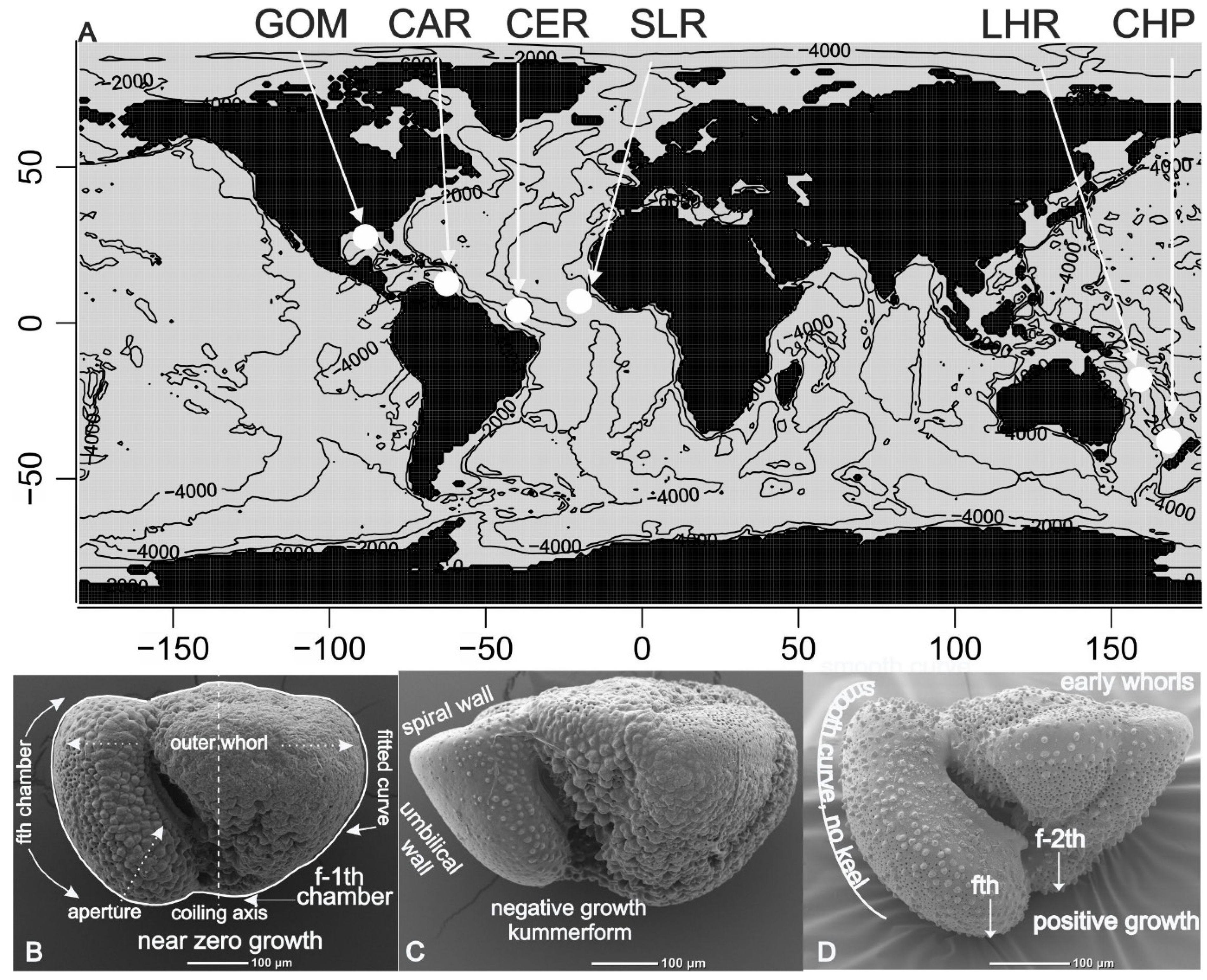
Figure 2.
The map displays the probabilities that specimens in the GOM sample, projected onto PC1:2 axes, belong to a normal (gaussian) shape population. Placed near the mode are specimens 1, 14, 20, 21 whose terminal growth ranges from weakly negative to positive (see Discussion).Their glohose form is close to the name bearers and they might be selected as representative specimens. Terminal growth in specimen 30 is strongly positive and is comparable to many in Figure 3. Like those, but rare in the GOM sample, it is crust-free.
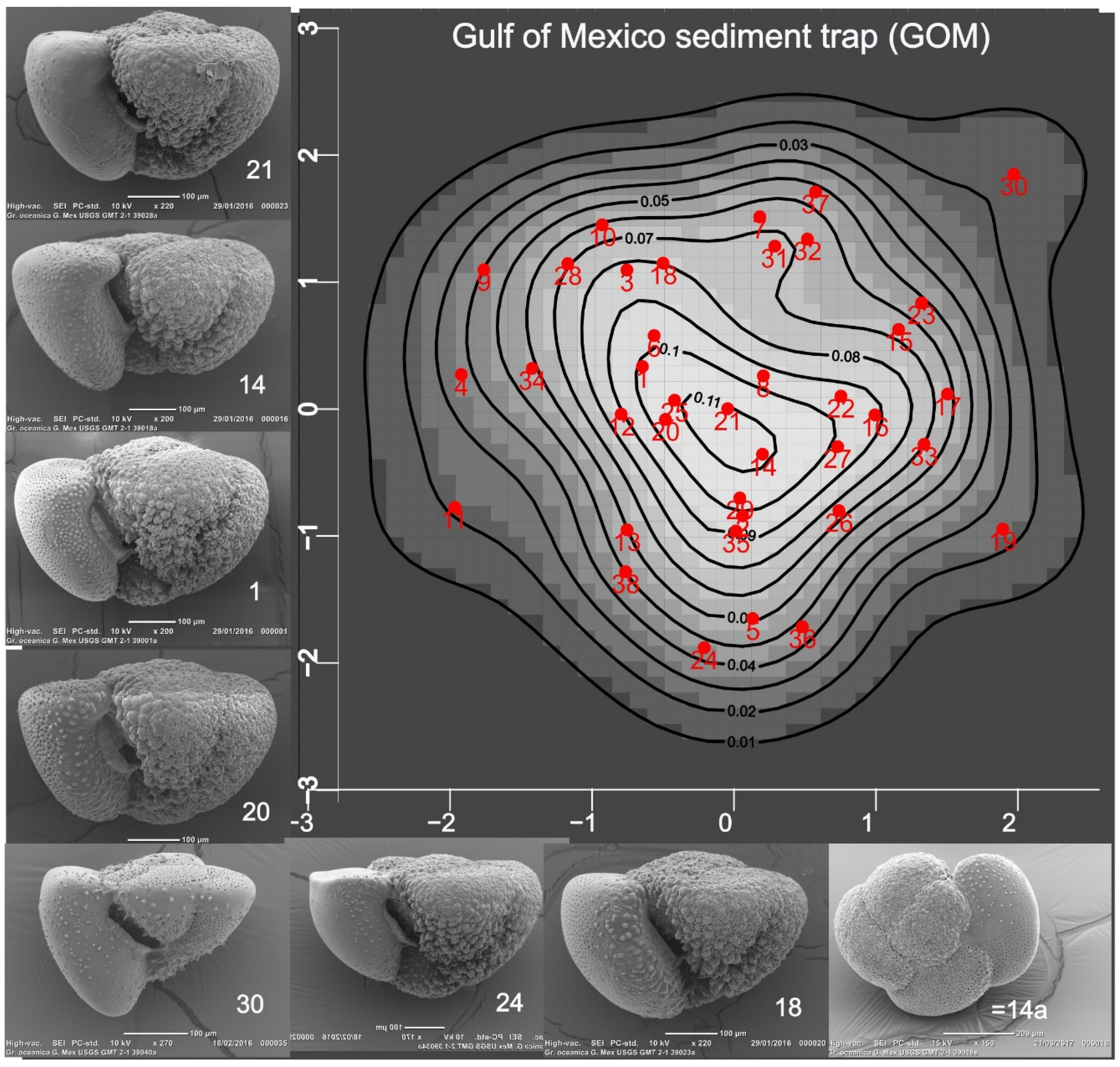
Figure 3.
The map displays the probabilities that specimens in the CAR sample, projected onto PC1:2 axes, belong to a normal (gaussian) shape population. All specimens show positive terminal stage growth (see Discussion). Specimens 4, 6, 7, and 22, placed near the well-defined mode, may be considered to be representative or voucher specimens for this population. The prominent cone formed by early whorls contributes to the displacement of specimen 19. Also distinguished is specimen 11 due to its greater width relative to axial height. Notably, only at the peripheral margin of early chambers of the outer whorl of specimens are pores covered by a calcitic veneer (Scott et al. 2015).
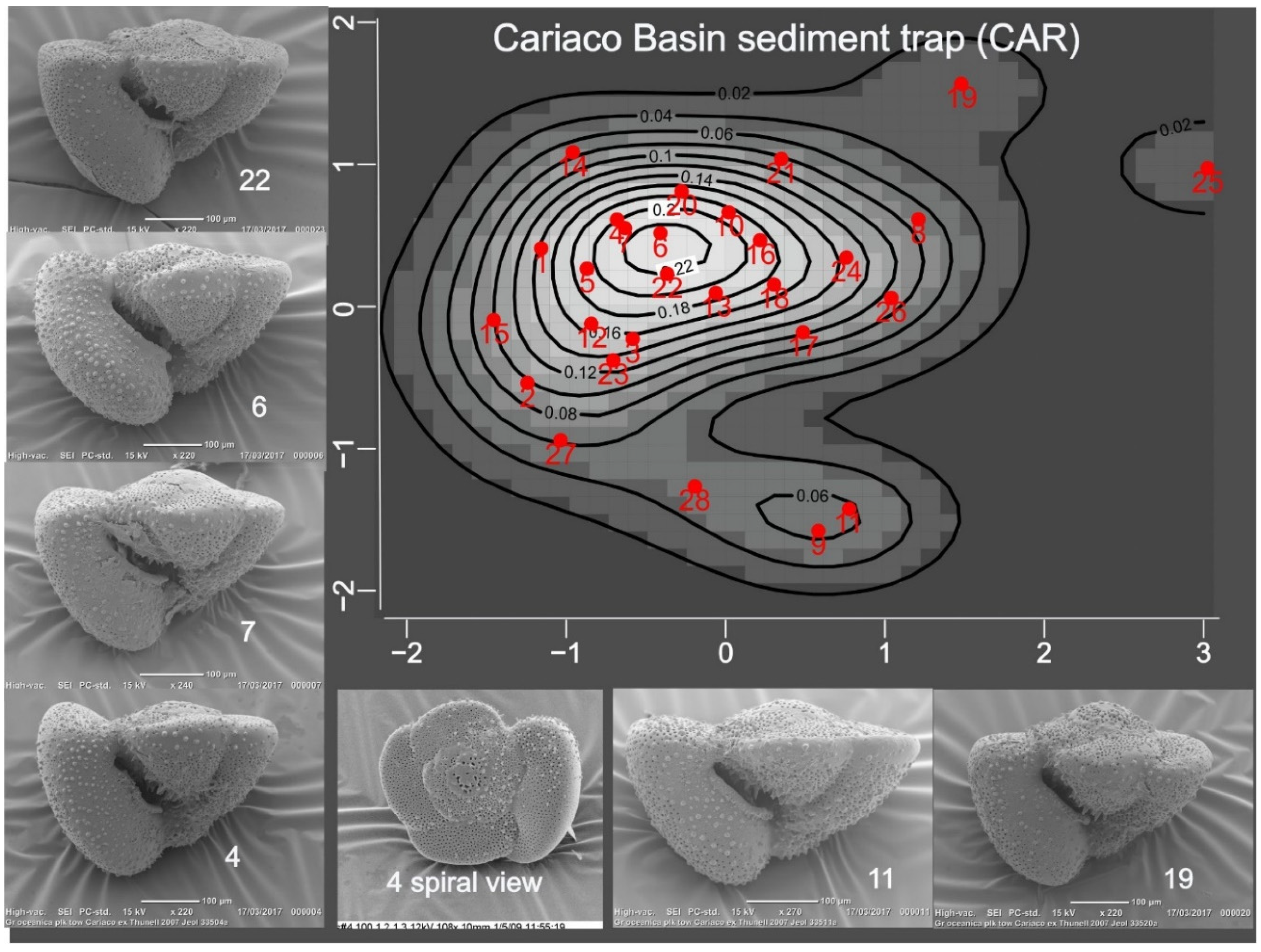
Figure 4.
The map displays the probabilities that specimens in the SLR sample, projected onto PC1:2 axes, belong to a normal (gaussian) shape population. Growth terminology is explained in Discussion. Specimens showing normal growth (1, 2, 11, 25) are near one weakly defined mode; their gently curved fth chamber profiles and absence of crust compare with specimens in CAR (Fig.3). Specimens 6, 19, 30 lie near another weakly defined mode: all display negative growth and are encrusted. While these data suggest that the shape population is possibly bimodal, the negative growth specimens are considered to form part of one taxonomic population.
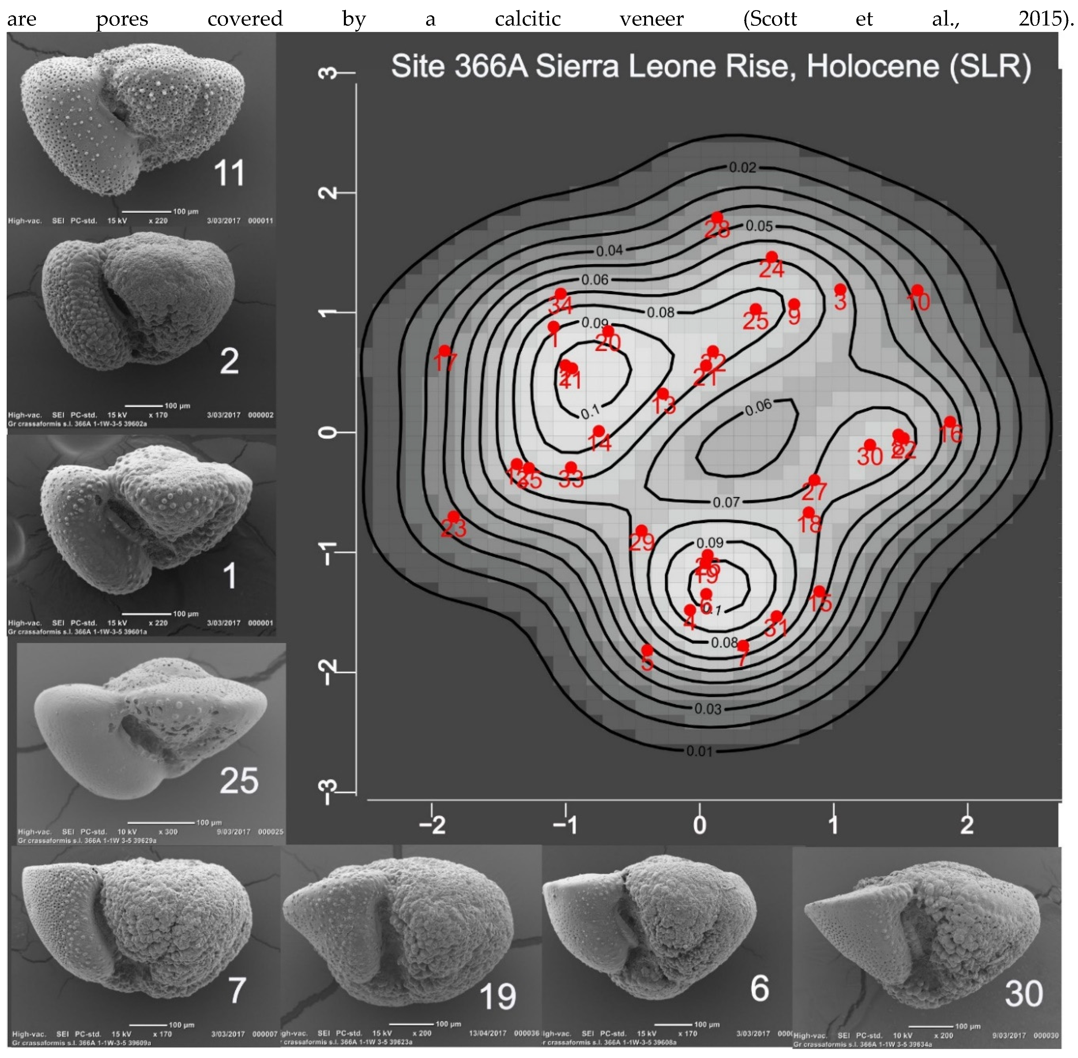
Figure 5.
The map displays the probabilities that specimens in the SLR sample, projected onto PC1:2 axes, belong to a normal (gaussian) shape population. Growth terminology is explained in Discussion. Specimens 10, 11, 14, and 21 have high probabilities and might be considered as representative or voucher specimens. All except #14 show negative growth of the terminal chamber. Specimen 23 is an example in which the periphery of the fth chamber is compressed; because such specimens are recognized as growth variants, they are accepted as part of the taxonomic concept. Specimen 8 is similarly interpreted; note its resemblance to some CAR specimens (Figure 3) . Whether specimen 19, an outlier in shape space, is within the taxonomic concept is uncertain.
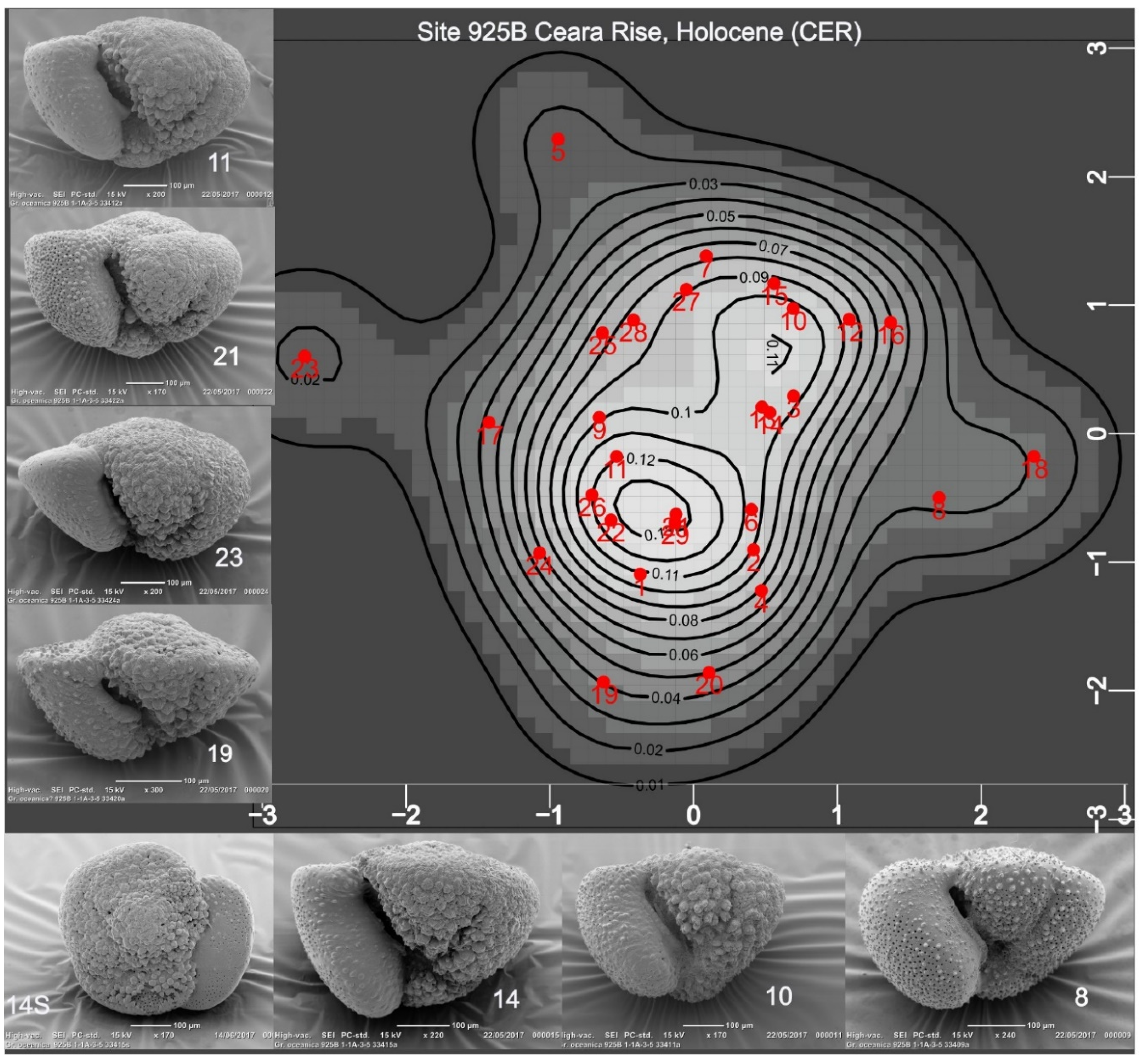
Figure 6.
A) Data ellipses for a procrustes analysis of pooled Gulf of Mexico (GOM), Cariaco Basin (CAR), Ceara Rise (CER). Sierra Leone Rise (SLR) samples, with the addition of the three named specimens of Truncorotalia oceanica. Most specimens are within the 95% data ellipse of their respective sample. Principal features are the partial intersections of GOM, CER and SLR ellipses and the offset of the CAR ellipse. B–D) named specimens of Globorotalia oceanica Cushman and Bermúdez 1949, which was described from bottom sediments off the north coast of Cuba.
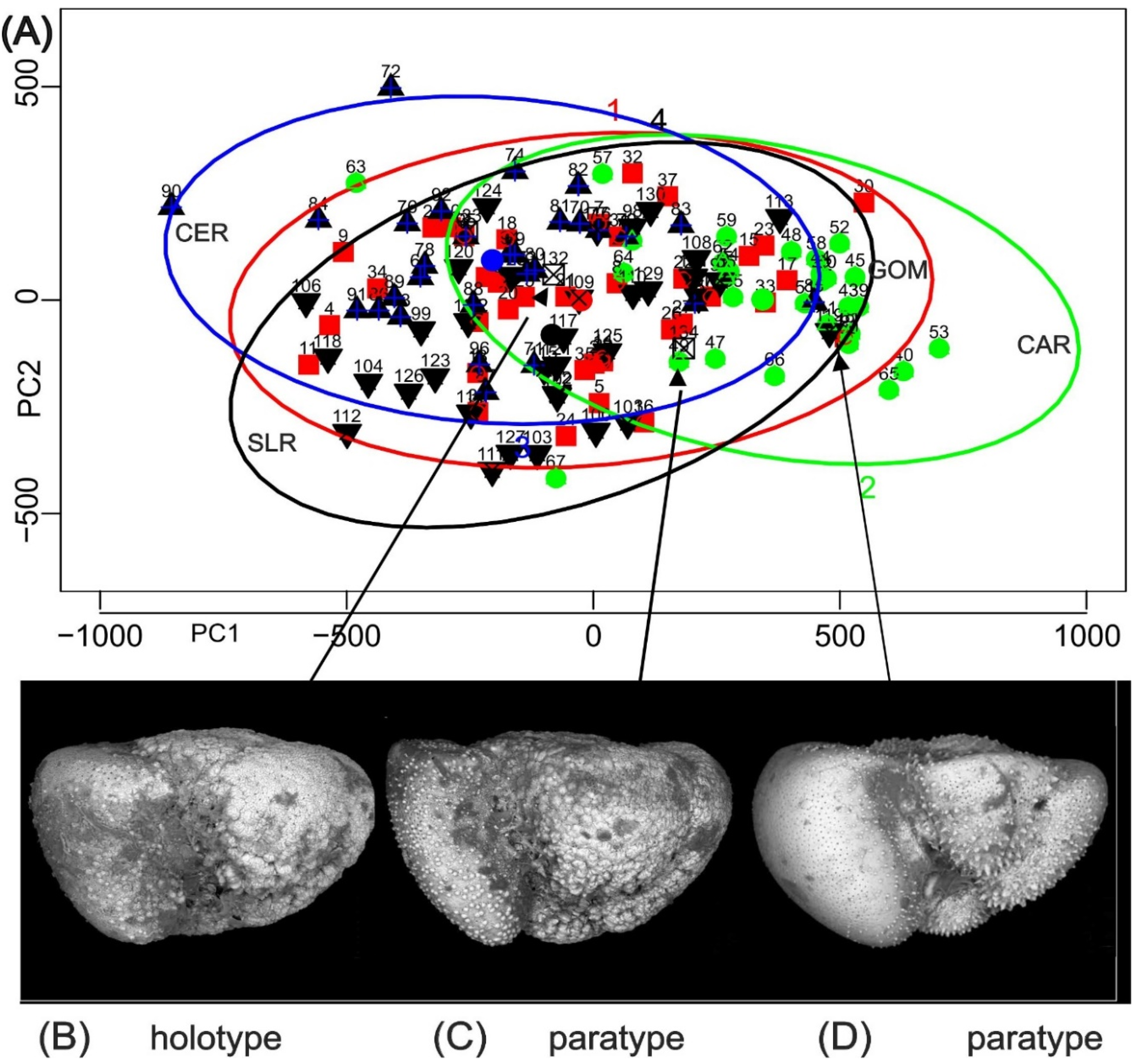
Figure 7.
A) Specimens near the center of B. B) The map displays the probabilities that specimens in the CHA sample, projected onto PC1:2 axes, belong to a normal (gaussian) shape population. C) Overlays of mean shapes computed with function testmeanshapes in R package shapes (available from https://CRAN.R-project.org/package=shapes) for CAR, GOM and CHA. D) Canonical scores computed for 12 harmonic amplitudes fitted to the data of Bicknell et al., (2018). Shown are scores for the basal Pliocene samples (Bicknell et al. 2018, Figure 2) that they identified as Truncorotalia crassaformis. The kernel density map B) samples a horizon in the near vicinity of their 4.82 Ma sample.
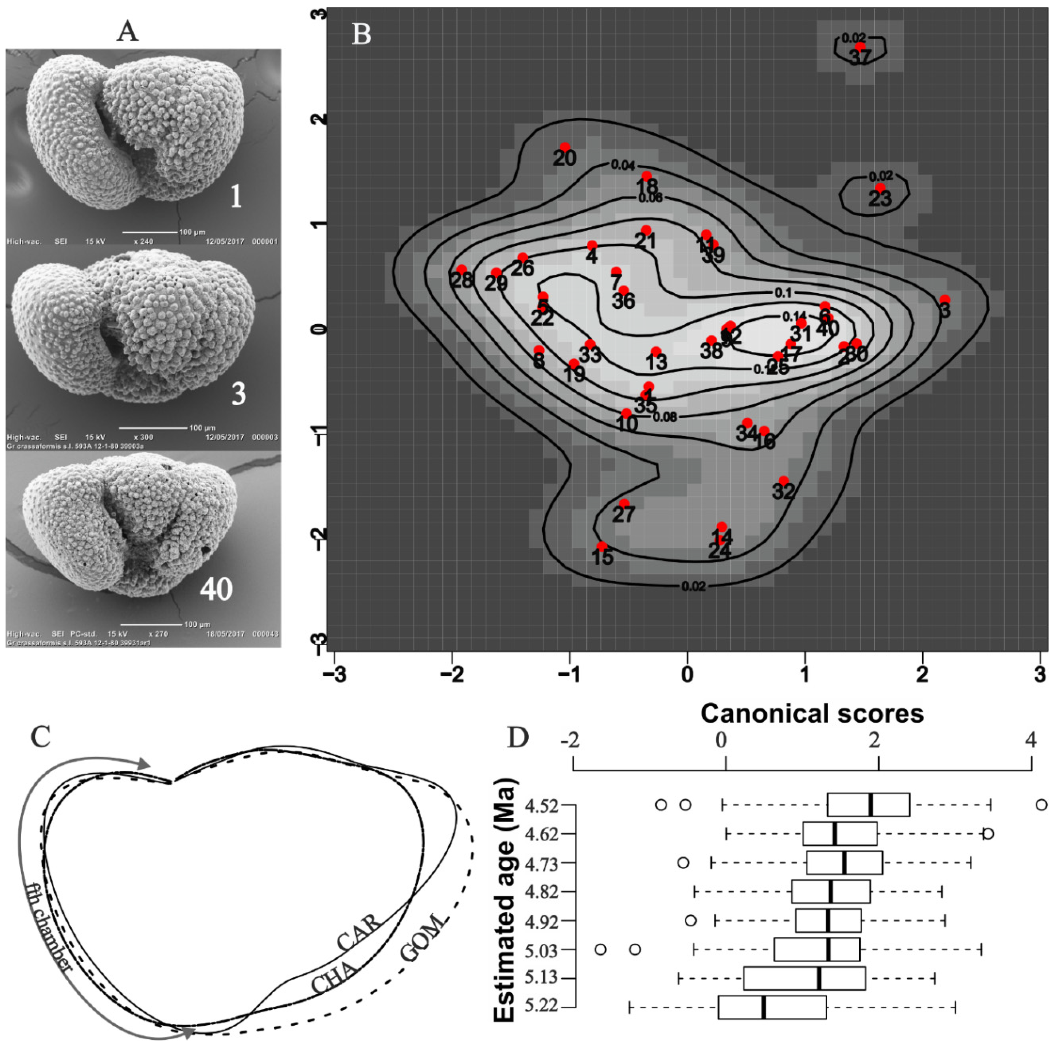
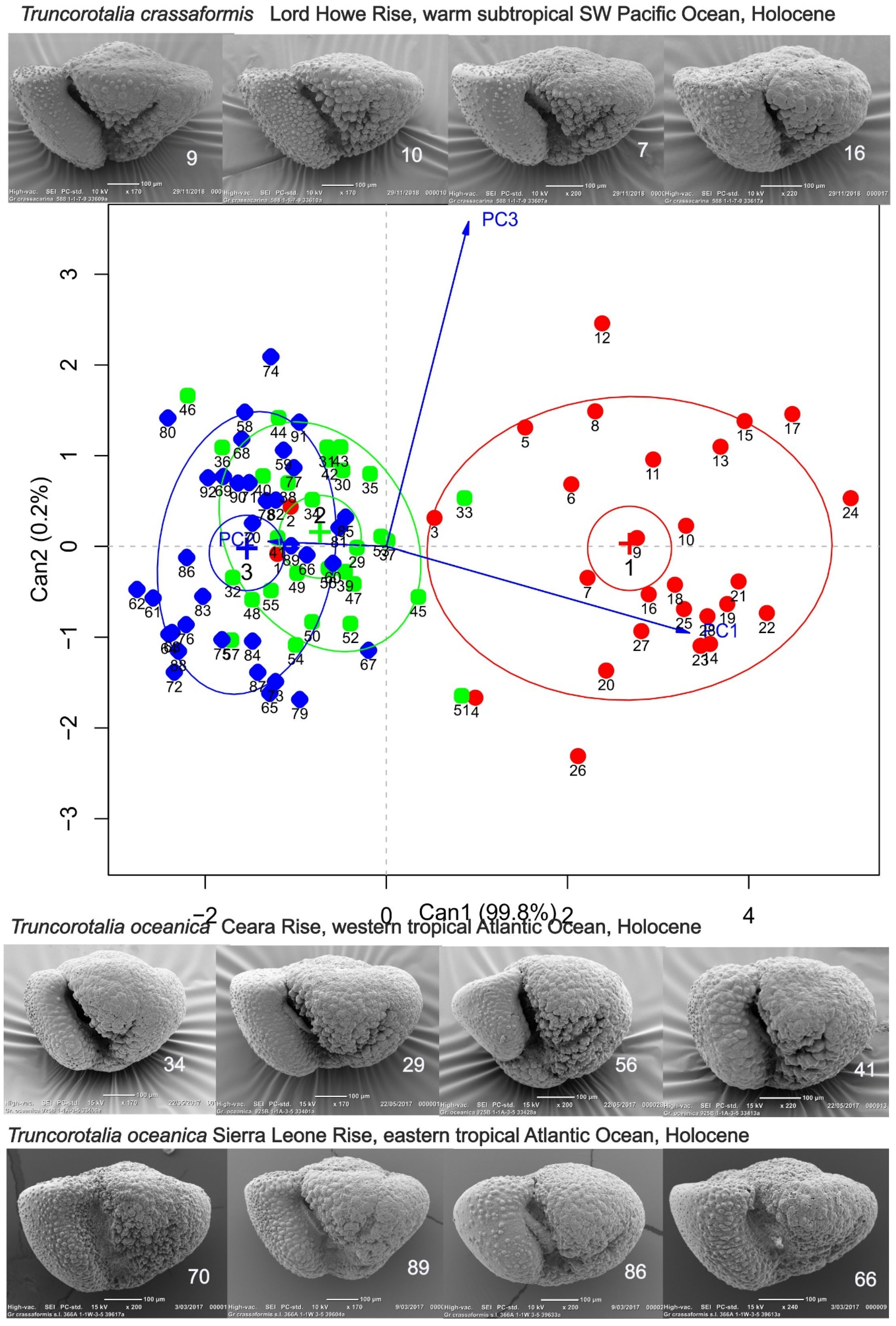
Figure 8.
Discrimination of Truncorotalia crassaformis from Truncorotalia oceanica using axial shape data for SLR and CER (tropical Atlantic Ocean) and LHR warm subtropical Southwest Pacific Ocean. A generalized canonical discriminant analysis (function candisc in R package candisc (available from https://CRAN.R-project.org/package=candisc) of data from a multivariate linear model uses PC1:3 projection data from the procrustes-processed samples. In this analysis almost all of the between-sample variation is accomodated on one axis which strongly discriminates LHR shells from those of CER and SLR.
Disclaimer/Publisher’s Note: The statements, opinions and data contained in all publications are solely those of the individual author(s) and contributor(s) and not of MDPI and/or the editor(s). MDPI and/or the editor(s) disclaim responsibility for any injury to people or property resulting from any ideas, methods, instructions or products referred to in the content. |
© 2025 by the authors. Licensee MDPI, Basel, Switzerland. This article is an open access article distributed under the terms and conditions of the Creative Commons Attribution (CC BY) license (http://creativecommons.org/licenses/by/4.0/).
Copyright: This open access article is published under a Creative Commons CC BY 4.0 license, which permit the free download, distribution, and reuse, provided that the author and preprint are cited in any reuse.


