Submitted:
17 February 2025
Posted:
18 February 2025
Read the latest preprint version here
Abstract
Accurate greenhouse gas (GHG) concentration forecasting is pivotal for evaluating climate policies, yet existing models face challenges in capturing multi-scale temporal patterns. To address this limitation, we propose MGGTSP-CAT, a novel multi-encoder framework that integrates daily and monthly data through an Input Attention encoder and an Autoformer encoder, enhanced by a Temporal Attention mechanism. Evaluated on NOAA datasets spanning five decades from Mauna Loa, Barrow, American Samoa, and Antarctica, MGGTSP-CAT outperforms 14 baseline models, achieving a Test_R² of 0.9627 and Test_MAPE of 1.47%. Crucially, the model demonstrates robustness in multi-step forecasting, with Test_R² declining by only 3.3% over ten steps—significantly lower than Transformer-based counterparts. These results underscore the framework’s capability to decouple short-term fluctuations from long-term trends, offering a reliable tool for cross-scale climate predictions and policy design.
Keywords:
Greenhouse Gas Forecasting
; Time Series Prediction
; Multi-scale Modeling
; Cross-Attention Mechanism
1. Introduction
Climate change is a global challenge impacting all of humanity, and greenhouse gas emissions data plays a crucial role in assessing the effectiveness of environmental policies and understanding the dynamic changes in the global climate system [1,2,3]. As a key parameter for quantifying climate system states, greenhouse gas concentration reflects the imbalance in the Earth's carbon cycle, far surpassing the significance of regional or national emissions data. By integrating diverse data sources, including atmospheric monitoring, satellite remote sensing, and ground observations, greenhouse gas concentrations provide accurate insights into human activity, ecosystem carbon sink capacity, and the effectiveness of climate policies. This information serves as a foundation for predicting global climate trends, supporting international climate negotiations, and aiding governments in optimizing emission reduction strategies and identifying critical points in the carbon peak process, ultimately enhancing climate governance [4].
Accurately capturing the balance between carbon sources and sinks is essential for reliable greenhouse gas concentration predictions. To improve prediction accuracy, multi-dimensional modeling approaches are employed to assess natural systems, human activities, policy interventions, and technological innovations. Policy analysis plays a vital role in evaluating international agreements like the Paris Agreement, carbon pricing reforms, and clean energy promotion, all of which shape emission intensity and carbon removal efficiency [5,6]. Historical data analysis, including trend decomposition and anomaly detection, unveils the interaction mechanisms between human activities and natural systems, especially near carbon cycle critical thresholds [7,8].
However, policy analysis and scenario simulations are often fraught with uncertainty due to their dependence on political will, economic transitions, and unpredictable factors like technology diffusion. Data analysis, in contrast, relies more heavily on observational data and scientific principles, offering a more stable and repeatable basis for prediction [9]. Despite the strong track record of traditional climate models, such as Global Circulation Models (GCMs) and Regional Climate Models (RCMs), these models struggle with accurately simulating short-term concentration fluctuations and fine-scale predictions. Smith et al. constructed a global climate model and made predictions for the next decade, significantly improving prediction accuracy [10]. However, these models still exhibit significant uncertainty, especially in characterizing short-term fluctuations and ecosystem feedback mechanisms, such as methane release due to permafrost thawing, which complicates their application in greenhouse gas forecasting.
With the growing demand for more precise climate predictions, data-driven approaches are becoming increasingly important. Machine learning models, such as Random Forests [11] and Gradient Boosting Decision Trees [12], have demonstrated their ability to handle complex, high-dimensional data, uncovering nonlinear relationships and identifying regional emission hotspots. For example, Zhang Jianxun et al. used the XGBoost algorithm to predict carbon emissions in urban expansion, highlighting the model's strength in predicting emissions for rapidly expanding megacities [13]. However, these models lack physical interpretability and are highly dependent on data quality, which can lead to biases in regions with sparse observation networks.
Recent breakthroughs in deep learning, particularly with architectures like Long Short-Term Memory (LSTM) [14] and Spatio-Temporal Graph Convolution Networks (STGCNs), have enhanced the prediction of greenhouse gas concentrations by capturing spatio-temporal correlations in atmospheric transport. Zhang Lei et al. demonstrated the use of CNN-LSTM for predicting soil organic carbon content, proving its effectiveness in regional carbon content forecasting [15]. Panja et al. developed the E-STGCN model for air quality forecasting in Delhi, India, achieving consistent performance across all seasons [16]. These models show promise but still face challenges, particularly in regions with limited data coverage and physical inconsistencies in extrapolated predictions. The Transformer architecture [17], with its self-attention mechanism, offers a new avenue for modeling global atmospheric transport, improving prediction accuracy for carbon emissions. Wu Xingping et al. implemented a temporal graph transformer-based attentional neural network to predict carbon emissions, achieving an 89.5% accuracy rate [18]. Despite its potential, the application of Transformers in climate prediction still requires further development, especially for extreme weather conditions.
Emerging deep learning models like Temporal Convolutional Networks (TCN) [19] , DA-RNN[20], Autoformer [21] have shown promise in modeling greenhouse gas concentrations by capturing seasonal periodicity and inter-annual variations in the carbon cycle. These architectures have yet to achieve breakthroughs in accuracy for emissions forecasting with a single time resolution.
To address the limitations of current models, this study introduces a multi-encoder fusion cross-scale forecasting framework, MGGTSP-CAT. By constructing a multi-time-resolution dataset, we integrate optimized Input-Attention and Autoformer Encoders, alongside LSTM, to extract features from both daily (short-term) and monthly (long-term) data. The multi-step forecasting is achieved through Temporal Attention, providing robust prediction accuracy and stability across different datasets. The proposed framework overcomes existing model limitations and sets a new standard for greenhouse gas concentration forecasting.
2. Materials and Methods
2.1. Data Curation
The dataset consists of daily carbon dioxide mole fraction data from continuous atmospheric measurements at stations in Mauna Loa (Hawaii), Barrow (Alaska), American Samoa, and Antarctica, collected by the National Oceanic and Atmospheric Administration (NOAA) [22]. The time span of the dataset is from July 24, 1973, to April 30, 2024, comprising 16,597 daily data points.
This dataset provides a benchmark platform for multi-scale prediction models, offering both high time resolution (daily) and long-term coverage (over half a century). The spatial distribution characteristics of different stations allow for effective validation of the model's ability to simultaneously model regional specificity (e.g., the Arctic amplification effect) and global consistency (e.g., long-term trends). In particular, the multi-modal features contained in the daily data, such as short-term fluctuations (influenced by weather systems) and long-term trends (driven by human emissions), offer an ideal experimental scenario for testing the performance of the multi-time-resolution hybrid architecture in decoupling temporal scales.
2.2. Methods
Overall, our model is divided into several parts: First, daily data is processed into monthly data for subsequent use (Input Phase). The encoding phase follows, where two different encoders are applied for different time resolution data: the Input-Attention Mechanism Encoder is used for daily data, and the Autoformer Encoder is used for monthly data. After all encoding is completed, the encoded daily and monthly data matrices are concatenated and fed into the decoder for decoding. The decoding phase utilizes a Temporal-Attention-based decoder to generate the output results (Output). The network diagram is shown in Figure 1.
2.2.1. Encoder
We first describe how to compute weekly and monthly data from daily data. For the daily input sequence ,monthly data is computed by averaging every 30 data points:
For daily data, we use an encoder based on Input Attention. The daily input sequence is processed through the Input Attention Mechanism, which includes the Input Attention Unit and LSTM units. The encoder uses this input attention mechanism to select and weight the input sequence, and uses LSTM units to generate hidden state sequences.
Specifically, for each time step , we first compute the basic hidden state through the LSTM unit:
Next, we calculate the attention weights , via the input attention mechanism and extract the new relevant driving sequence:
Using the new driving sequence, we update the hidden state:
where is the LSTM unit, and its internal computation is as follows:
where represents the activation function, and represents element-wise multiplication., are weight matrices, and are bias vectors.
Thus, we obtain the hidden state sequence for daily data:
For monthly data, we use the Autoformer Encoder. The monthly input sequence is processed Autoformer Encoder , which mainly consists of the series decomposition block (Series Decomp), auto-correlation mechanism (Auto-Correlation), and feed-forward neural network (Feed Forward). The encoder uses these components to process the input sequence, extract long-term trend information, and model seasonal patterns, thus generating the hidden state sequence for monthly data.
Specifically, for each time step , we first process the input sequence through the series decomposition block. Since directly decomposing future sequences is not realistic, Autoformer proposes the series decomposition block as an internal operation to progressively extract the long-term stable trend from the predicted intermediate hidden variables. The process smoothes periodic fluctuations through moving averages (using AvgPool and Padding operations) to highlight long-term trends. For an input sequence of length , the calculation is as follows:
where represent the seasonal part and the extracted trend-periodic part. We summarize this process in the internal block .
Next, the output of the auto-correlation mechanism is calculated. The auto-correlation mechanism identifies cycle-based dependencies and aggregates similar sub-series through time-delay aggregation. First, we introduce two basic mechanisms: cycle-based dependencies and time-delay aggregation, then extend them to single-head and multi-head auto-correlation mechanism outputs.
Cycle-based Dependencies: For a real discrete-time process , the auto-correlation is computed as follows:
(In practical computations, we select the most likely periodicities , where , with being a hyperparameter)This autocorrelation reflects the temporal similarity between and its -lagged series , thus capturing the periodic dependencies.
Time-delay Aggregation: Based on the selected time delays , the series is rolled using a operation to align similar subsequences that share the same phase of the estimated period. These subsequences are then aggregated using a -normalized confidence score.
Thus, for the single-head case and a time series of length , after projecting the sequence to obtain the query , key and value matrices, the auto-correlation mechanism is computed as follows:
For multi-head mechanisms with hidden variable channels , and number of heads , the calculation process is:
Thus, the calculation of the auto-correlation mechanism output is completed.
The output of the auto-correlation mechanism is further transformed through a feed-forward neural network. The computation of the feed-forward network is similar to the Transformer Encoder (including fully connected layers with an activation function, such as ReLU)
Let the output of the auto-correlation mechanism or be , then:
Finally, the output hidden state is obtained through residual connections and layer normalization:
Thus, we obtain the hidden state sequence for monthly data
2.2.2. Decoder
After encoding, the hidden state sequences from the two encoders are concatenated to form the final hidden sequence :
This concatenated sequence is then passed into the Temporal Mechanism to decode the final prediction sequence. The Temporal Mechanism includes the Temporal Attention Unit and LSTM unit, where the Temporal Attention Unit is used to select the hidden states of the encoders, and the LSTM unit updates the decoder's hidden state and outputs the final prediction .
Specifically, for each time step , we first compute the time attention scores:
Then, we calculate the attention weights:
Next, we compute the context vector:
The decoder input is combined with the context vector to generate the new input:
The decoder's hidden state is updated:
Finally, we output the prediction:
where is the LSTM unit, and its internal computation is:
where represents the activation function, denotes element-wise multiplication, and are the weight matrices and weight vectors, while and are the bias vectors.
2.2.3. Metric
The following are the formulas for calculating the goodness-of-fit of the model:
, Coefficient of Determinatio:
where represents the true value, represents the predicted value, represents the mean of the true values, represents the sample size.
, Mean Squared Error:
where represents the true value, represents the predicted value, represents the sample size.
, Mean Absolute Error:
where represents the true value, represents the predicted value, represents the sample size.
, Mean Absolute Percentage Error:
where represents the true value, represents the predicted value, represents the sample size.
3. Results
3.1. Overall Performances
The proposed MGGTSP-CAT framework demonstrates superior predictive capabilities across all evaluation metrics compared to 14 baseline models. As summarized in Table 1, MGGTSP-CAT achieves the highest Test_R² of 0.9627, significantly outperforming DARNN (0.9519) and Autoformer (0.9480). This improvement is attributed to the model’s ability to effectively integrate multi-scale temporal patterns, capturing both short-term fluctuations (e.g., daily weather variations) and long-term trends (e.g., seasonal and policy-driven changes). The model also exhibits the lowest error metrics, with Test_MSE = 0.000288 (22.7% reduction vs. DARNN) and Test_MAE = 0.0116 (11.3% improvement vs. Autoformer). Notably, the Test_MAPE of 1.47% confirms the model’s robustness in minimizing percentage-based deviations, which is critical for practical applications where relative error margins are more meaningful than absolute values. Figure 2 visually illustrates the alignment between predicted and true values over ten forecasting steps.
3.2. Single Step
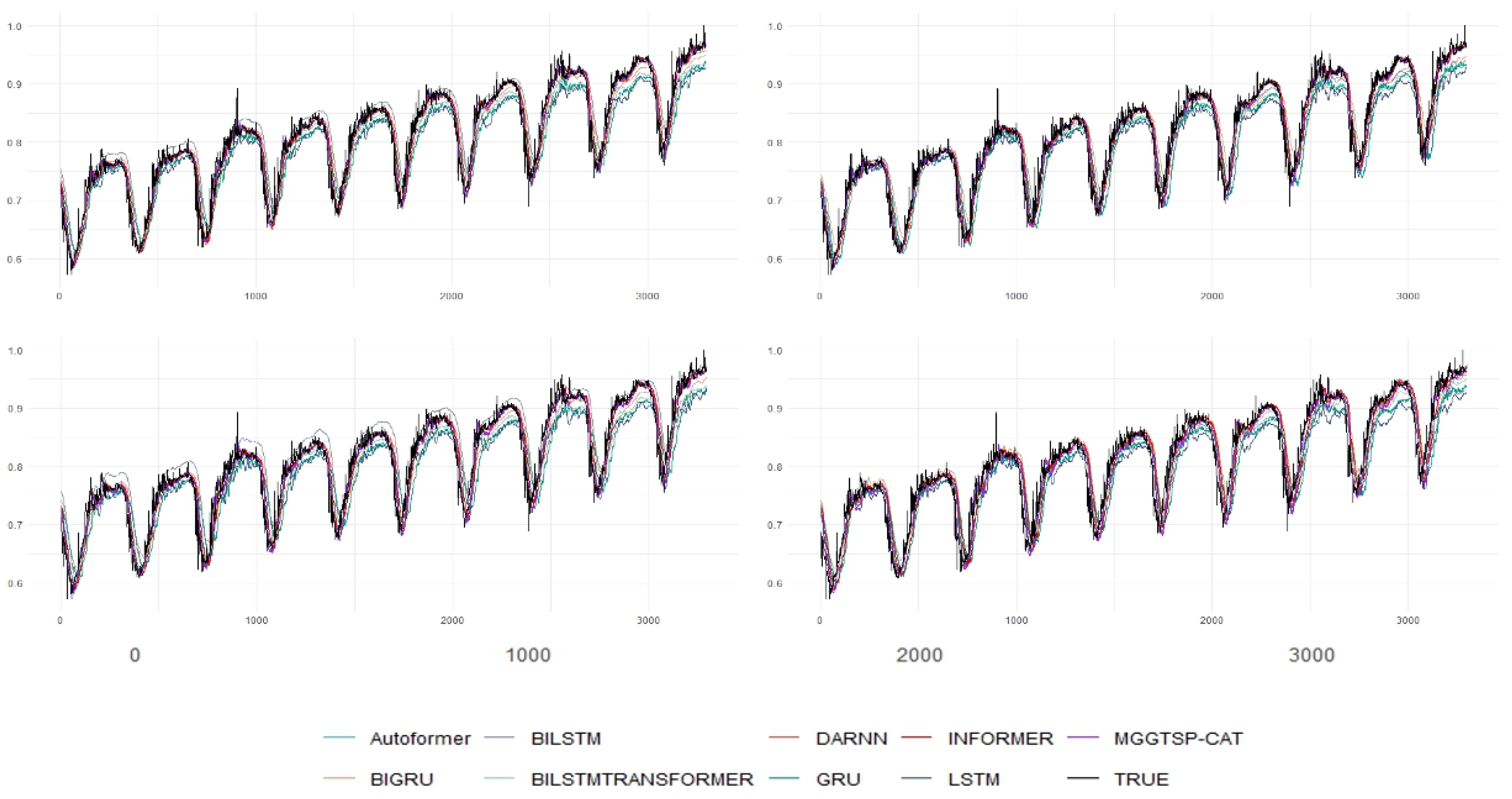
The model’s stability under extended forecasting horizons is rigorously validated through multi-step experiments (Table 2, Table 3, Table 4 and Table 5). From Step 1 to Step 10, MGGTSP-CAT maintains a gradual decline in Test_R² (0.9788 → 0.9470, Δ = 3.3%), outperforming DARNN (Δ = 3.9%) and Autoformer (Δ = 4.2%). This gradual decline indicates that the model’s Temporal Attention mechanism effectively mitigates error accumulation, a common challenge in long-term forecasting. Critically, the rate of error accumulation remains constrained: Test_MSE increases from 0.000163 (Step 1) to 0.000410 (Step 10), representing a 2.5× rise, compared to Autoformer’s 2.3× increase (0.000236 → 0.000554). This advantage is particularly evident in Steps 5–10, where traditional LSTM/GRU models exhibit significant performance degradation due to their inability to model long-term dependencies effectively. Figure 3 further demonstrates the model’s ability to preserve prediction accuracy across diverse baseline comparisons, particularly in Steps 5–10, where traditional LSTM/GRU models exhibit significant performance degradation. The model’s ability to maintain high accuracy over extended forecasting horizons is a significant improvement over existing methods, which often struggle with error propagation in multi-step predictions.
3.3. Robustness Against Baseline Models
MGGTSP-CAT consistently outperforms both classical and state-of-the-art architectures. For instance, the Test_R² gap between MGGTSP-CAT and the second-best model (DARNN) widens from 0.7% at Step 1 to 1.4% at Step 10 (Table 2). Similarly, error metrics such as Test_MAE (0.01446 at Step 10) remain 8.5% lower than DARNN (0.01581), underscoring the efficacy of the multi-scale fusion mechanism in mitigating error propagation. The model’s advantage is particularly pronounced in high-variability scenarios, as evidenced by its stable MAPE trajectory (1.07% → 1.42% over ten steps), contrasting sharply with the erratic performance of Transformer-based models like BiTransformer_LSTM. This robustness is critical for real-world applications, where models must perform reliably under diverse and often unpredictable conditions. Additionally, MGGTSP-CAT’s computational efficiency is a notable advantage, as it achieves these results with lower computational overhead compared to Transformer-based models, making it more feasible for deployment in resource-constrained environments.The predicted values and true values of the nine best models participating in the experiment for Step 1, Step 2, Step 5, and Step 10 are shown in Figure 3.
Figure 3.
The predicted values and true values of the nine best models.
4. Discussions
The MGGTSP-CAT framework introduces a structured approach to multi-scale greenhouse gas (GHG) concentration forecasting by integrating daily and monthly temporal patterns through a dual-encoder architecture. This design addresses a critical challenge in existing models, which often struggle to reconcile short-term variability with long-term trends. By employing an Input Attention encoder for high-frequency daily data and an Autoformer encoder for low-frequency monthly data, the model effectively captures both transient weather-driven fluctuations (e.g., synoptic-scale atmospheric changes) and persistent seasonal or policy-driven trends (e.g., annual emission cycles). The experimental results validate this approach, with MGGTSP-CAT achieving a Test_R² of 0.9627, outperforming baseline models such as DARNN (Test_R² = 0.9519) and Autoformer (Test_R² = 0.9480).
A notable strength of the model lies in its stability during multi-step forecasting. Over a ten-step horizon, the Test_R² declines by only 3.3% (from 0.9788 to 0.9470), compared to sharper deteriorations in Transformer-based models like BiTransformer_LSTM (Δ = 5.7%) and traditional sequential architectures like LSTM (Δ = 12.7%). This robustness is attributed to the Temporal Attention mechanism, which dynamically weights historical states to minimize error propagation—a common issue in long-term prediction tasks. For instance, the Test_MSE increases by a factor of 2.5 from Step 1 to Step 10 (0.000163 → 0.000410), a slower escalation than Autoformer’s 2.3-fold rise (0.000236 → 0.000554), despite the latter’s reliance on self-attention for global dependencies.
The framework’s computational efficiency further enhances its practicality. By decoupling daily and monthly processing, MGGTSP-CAT reduces computational overhead compared to monolithic Transformer architectures, which require quadratic memory for self-attention over long sequences. This efficiency is critical for real-world deployment, particularly in regions with limited computational resources. Additionally, the model’s ability to handle multi-modal temporal features—such as isolating short-term noise from long-term signals—proves advantageous in complex scenarios like Arctic monitoring, where rapid temperature shifts and multi-decadal warming trends coexist.
While the current evaluation focuses on CO₂ data from well-instrumented stations , the model’s architecture is extensible to other GHGs (e.g., CH₄, N₂O) and heterogeneous data sources, such as satellite observations or urban sensor networks. Future work could explore integrating exogenous variables (e.g., economic activity indices, land-use changes) to enhance scenario-based forecasting for policymakers. Nevertheless, the framework’s reliance on continuous high-resolution input data highlights the importance of maintaining robust observational infrastructure, particularly in underrepresented regions.
5. Conclusions
This study presents an innovative multi-attention encoder model based on cross-time resolution, which combines daily and monthly data at different time scales and processes them through specific encoder architectures. Specifically, the model employs the Input Attention Mechanism to process daily data and the Autoformer Encoder to handle monthly data. Subsequently, the features extracted from these different time resolutions are concatenated and decoded through the Temporal Mechanism to generate the final prediction results. This approach provides a more accurate and robust solution for cross-scale forecasting of greenhouse gas concentrations and offers significant support for more complex climate models.
The contributions of this study are as follows:
- 1)
- A greenhouse gas dataset covering multiple global major climate monitoring stations was created. The data is sourced from long-term monitoring stations in Mauna Loa (Hawaii), Barrow (Alaska), American Samoa, and Antarctica, spanning over half a century [22]. This dataset not only offers high temporal resolution (daily data) but also effectively reflects global climate change trends, providing a solid experimental foundation for cross-scale climate forecasting.
- 2)
- An innovative fusion of the model's time resolution with the characteristics of greenhouse gas data. This study designs a multi-encoder fusion architecture that integrates the characteristics of different time resolution data. The Input Attention Mechanism and Autoformer Encoder are used to extract features from daily and monthly data, respectively, while the Temporal Attention Mechanism further enhances the model’s ability to integrate information across different time scales. This method effectively captures the multi-scale features of greenhouse gas concentration changes, improving the model’s adaptability and accuracy in both short-term and long-term climate predictions.
- 3)
- Exceptional accuracy and stability of the model. The experimental results show that the proposed model exhibits outstanding performance in prediction tasks across multiple climate monitoring stations, especially in high-variability daily data. The model can accurately capture key change patterns and provide stable and reliable predictions. For both short-term and long-term predictions at different time scales, the model performs excellently, showing less fluctuation in prediction results and significantly improving stability compared to other existing methods.
- 4)
- Future research could further extend the application of the model by considering more types of greenhouse gas monitoring data and a wider range of geographical areas. The effectiveness and generalization ability of the model under different climate conditions could be explored. Additionally, the model could be applied to the prediction of various climate events, further enhancing its predictive accuracy and practical application value.
Author Contributions
H.W. contributed to conceptualization, data curation, software, methodology, visualization, writing—original draft preparation, Y.M. contributed to conceptualization, resources, writing—review and editing; J.R. contributed to conceptualization, data curation and software, All authors have read and agreed to the published version of the manuscript.
Funding
This research received no external funding
Institutional Review Board Statement
Not applicable
Informed Consent Statement
Not applicable
Data Availability Statement
The data presented in this study are available on request from the first author.
Conflicts of Interest
The authors declare no conflicts of interest.
References
- Barnett, J. Security and Climate Change. Global Environmental Change 2003, 13, 7–17. [Google Scholar] [CrossRef]
- Adedeji, O.; Reuben, O.; Olatoye, O. Global Climate Change. Journal of Geoscience and Environment Protection 2014, 2, 114–122. [Google Scholar] [CrossRef]
- Jeffry, L.; Ong, M.Y.; Nomanbhay, S.; Mofijur, M.; Mubashir, M.; Show, P.L. Greenhouse Gases Utilization: A Review. Fuel 2021, 301, 121017. [Google Scholar] [CrossRef]
- Ledley, T.S.; Sundquist, E.T.; Schwartz, S.E.; Hall, D.K.; Fellows, J.D.; Killeen, T.L. Climate Change and Greenhouse Gases. Eos, Transactions American Geophysical Union 1999, 80, 453–458. [Google Scholar] [CrossRef]
- Selin, H.; VanDeveer, S.D. Political Science and Prediction: What’s Next for U.S. Climate Change Policy? Review of Policy Research 2007, 24, 1–27. [Google Scholar] [CrossRef]
- Patnaik, S. A Cross-Country Study of Collective Political Strategy: Greenhouse Gas Regulations in the European Union. J Int Bus Stud 2019, 50, 1130–1155. [Google Scholar] [CrossRef]
- Narang, R.; Khan, A.M.; Goyal, R.; Gangopadhyay, S. Harnessing Data Analytics and Machine Learning to Forecast Greenhouse Gas Emissions. European Association of Geoscientists & Engineers, 14 November 2023; 2023, pp. 1–5. [Google Scholar]
- Kasatkin, A.J.; Krinitskiy, M.A. Machine Learning Techniques for Anomaly Detection in High-Frequency Time Series of Wind Speed and Greenhouse Gas Concentration Measurements. Moscow Univ. Phys. 2023, 78, S138–S148. [Google Scholar] [CrossRef]
- Emami Javanmard, M.; Ghaderi, S.F. A Hybrid Model with Applying Machine Learning Algorithms and Optimization Model to Forecast Greenhouse Gas Emissions with Energy Market Data. Sustainable Cities and Society 2022, 82, 103886. [Google Scholar] [CrossRef]
- Smith, D.M.; Cusack, S.; Colman, A.W.; Folland, C.K.; Harris, G.R.; Murphy, J.M. Improved Surface Temperature Prediction for the Coming Decade from a Global Climate Model. Science 2007. [CrossRef] [PubMed]
- Sun, H.; Liang, L.; Wang, C.; Wu, Y.; Yang, F.; Rong, M. Prediction of the Electrical Strength and Boiling Temperature of the Substitutes for Greenhouse Gas SF₆ Using Neural Network and Random Forest. IEEE Access 2020, 8, 124204–124216. [Google Scholar] [CrossRef]
- Cai, W.; Wei, R.; Xu, L.; Ding, X. A Method for Modelling Greenhouse Temperature Using Gradient Boost Decision Tree. Information Processing in Agriculture 2022, 9, 343–354. [Google Scholar] [CrossRef]
- Zhang, J.; Zhang, H.; Wang, R.; Zhang, M.; Huang, Y.; Hu, J.; Peng, J. Measuring the Critical Influence Factors for Predicting Carbon Dioxide Emissions of Expanding Megacities by XGBoost. Atmosphere 2022, 13, 599. [Google Scholar] [CrossRef]
- Sak, H.; Senior, A.; Beaufays, F. Long Short-Term Memory Recurrent Neural Network Architectures for Large Scale Acoustic Modeling. In Proceedings of the Interspeech 2014; ISCA, 14 September 2014; pp. 338–342. [Google Scholar]
- Zhang, L.; Cai, Y.; Huang, H.; Li, A.; Yang, L.; Zhou, C. A CNN-LSTM Model for Soil Organic Carbon Content Prediction with Long Time Series of MODIS-Based Phenological Variables. Remote Sensing 2022, 14, 4441. [Google Scholar] [CrossRef]
- Panja, M.; Chakraborty, T.; Biswas, A.; Deb, S. E-STGCN: Extreme Spatiotemporal Graph Convolutional Networks for Air Quality Forecasting; 2024. [Google Scholar]
- Vaswani, A.; Shazeer, N.; Parmar, N.; Uszkoreit, J.; Jones, L.; Gomez, A.N.; Kaiser, L.; Polosukhin, I. Attention Is All You Need; 2023. [Google Scholar]
- Wu, X.; Yuan, Q.; Zhou, C.; Chen, X.; Xuan, D.; Song, J. Carbon Emissions Forecasting Based on Temporal Graph Transformer-Based Attentional Neural Network. Journal of Computational Methods in Sciences and Engineering 2024, 24, 1405–1421. [Google Scholar] [CrossRef]
- Hewage, P.; Behera, A.; Trovati, M.; Pereira, E.; Ghahremani, M.; Palmieri, F.; Liu, Y. Temporal Convolutional Neural (TCN) Network for an Effective Weather Forecasting Using Time-Series Data from the Local Weather Station. Soft Comput 2020, 24, 16453–16482. [Google Scholar] [CrossRef]
- Qin, Y.; Song, D.; Chen, H.; Cheng, W.; Jiang, G.; Cottrell, G. A Dual-Stage Attention-Based Recurrent Neural Network for Time Series Prediction; 2017. [Google Scholar]
- Wu, H.; Xu, J.; Wang, J.; Long, M. Autoformer: Decomposition Transformers with Auto-Correlation for Long-Term Series Forecasting. In Proceedings of the Advances in Neural Information Processing Systems; Curran Associates, Inc., 2021; Vol. 34; pp. 22419–22430. [Google Scholar]
- Thoning, K.W.; Crotwell, A.M.; Mund, J.W. Atmospheric Carbon Dioxide Dry Air Mole Fractions from continuous measurements at Mauna Loa, Hawaii, Barrow, Alaska, American Samoa and South Pole, 1973-present. Version 2024-08-15; National Oceanic and Atmospheric Administration (NOAA), Global Monitoring Laboratory (GML): Boulder, Colorado, USA, 2024; Volume -15. [Google Scholar] [CrossRef]
Figure 1.
MGGTSP-CAT Encoding and Decoding Mechanism.
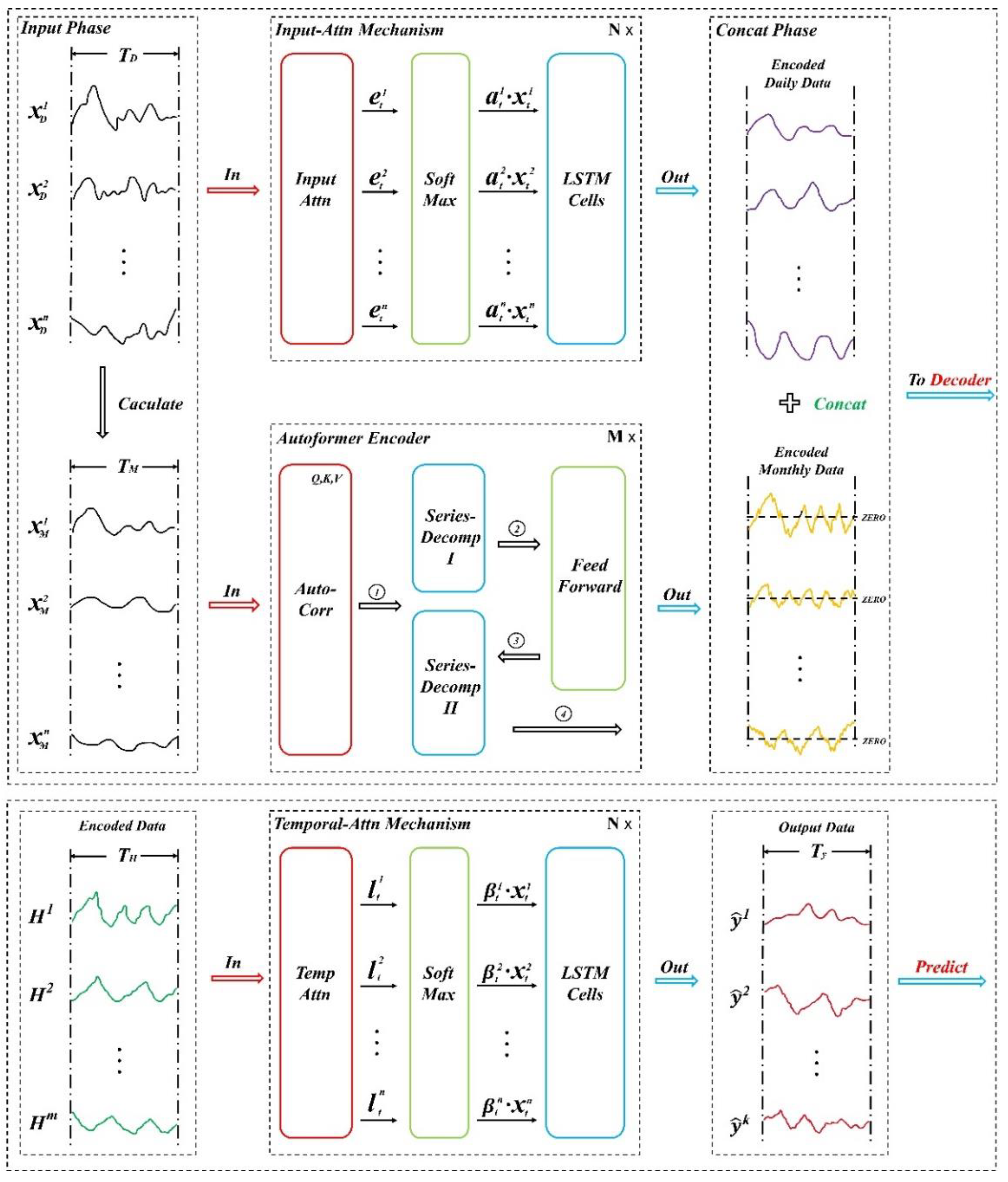
Figure 2.
Ten Steps MGGTSP-CAT Predicted Values and True Values on dataset.
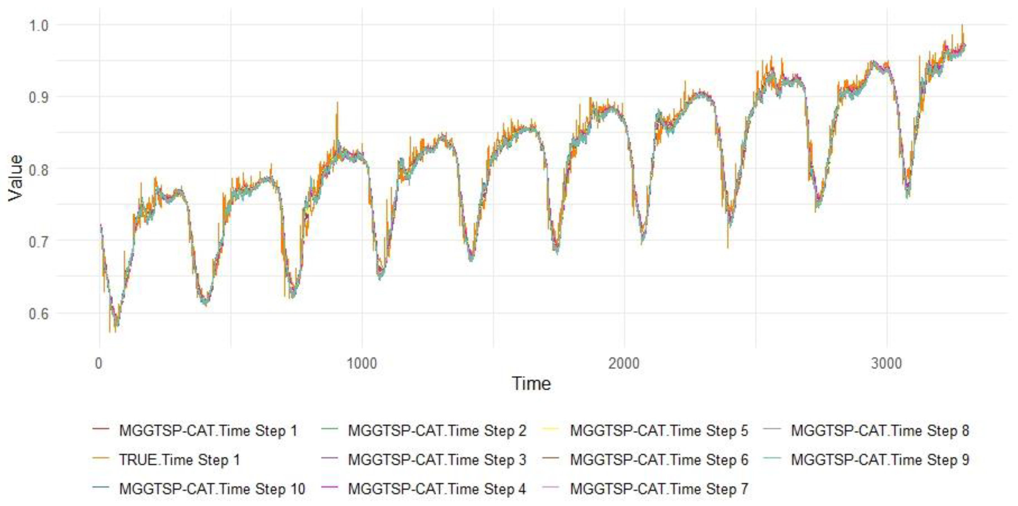

Table 1.
All test set data of 15 models.
| Model | Test_MSE | Test_MAE | Test_R² | Test_MAPE |
|---|---|---|---|---|
| MGGTSP | 0.0002878 | 0.0116377 | 0.9627339 | 0.0147310 |
| DARNN | 0.0003716 | 0.0131211 | 0.9518857 | 0.0167605 |
| Autoformer | 0.0004013 | 0.0136400 | 0.9480379 | 0.0174719 |
| TCN | 0.0004571 | 0.0146228 | 0.9408147 | 0.0187982 |
| BiTransfomer_LSTM | 0.0005962 | 0.0184426 | 0.9227868 | 0.0231243 |
| Informer | 0.0006874 | 0.0182407 | 0.9109833 | 0.0236269 |
| LSTM | 0.0008636 | 0.0243913 | 0.8881612 | 0.0295327 |
| Bi_GRU | 0.0012059 | 0.0257306 | 0.8438375 | 0.0333236 |
| Bi_LSTM | 0.0012679 | 0.0260454 | 0.8358032 | 0.0338971 |
| GRU | 0.0012723 | 0.0292467 | 0.8352157 | 0.0367302 |
| RNN | 0.0013303 | 0.0306885 | 0.8276975 | 0.0373433 |
| CNN1D | 0.0018290 | 0.0351233 | 0.7631485 | 0.0422021 |
| Bi_RNN | 0.0025301 | 0.0413129 | 0.6723005 | 0.0485256 |
| CNN1D_LSTM | 0.0028931 | 0.0447957 | 0.6253179 | 0.0527006 |
| ANN | 0.0043728 | 0.0612601 | 0.4336226 | 0.0744804 |
Table 2.
10 step Test_R² data of 15 models participating in the experiment.
| Model | STEP1 | STEP2 | STEP3 | STEP4 | STEP5 | STEP6 | STEP7 | STEP8 | STEP9 | STEP10 |
|---|---|---|---|---|---|---|---|---|---|---|
| MGGTSP | 0.97878 | 0.97443 | 0.97074 | 0.96684 | 0.96564 | 0.96125 | 0.95805 | 0.95458 | 0.95005 | 0.94698 |
| DARNN | 0.97102 | 0.96757 | 0.96023 | 0.95383 | 0.95822 | 0.94851 | 0.94829 | 0.94355 | 0.93422 | 0.93341 |
| Autoformer | 0.96930 | 0.96559 | 0.95608 | 0.94813 | 0.95578 | 0.94324 | 0.94548 | 0.93990 | 0.92843 | 0.92844 |
| TCN | 0.96514 | 0.96146 | 0.94898 | 0.93800 | 0.95049 | 0.93385 | 0.93957 | 0.93361 | 0.91780 | 0.91926 |
| BiTransfomer _LSTM |
0.94296 | 0.92876 | 0.93205 | 0.92333 | 0.91395 | 0.94672 | 0.90693 | 0.91436 | 0.91156 | 0.90723 |
| Informer | 0.94596 | 0.94410 | 0.92072 | 0.89425 | 0.92664 | 0.89500 | 0.91480 | 0.90963 | 0.87846 | 0.88027 |
| LSTM | 0.91190 | 0.90502 | 0.90029 | 0.88391 | 0.89488 | 0.90956 | 0.88113 | 0.85724 | 0.86588 | 0.87179 |
| Bi_GRU | 0.88297 | 0.83717 | 0.90740 | 0.88788 | 0.84569 | 0.76714 | 0.91339 | 0.78506 | 0.74577 | 0.86590 |
| Bi_LSTM | 0.85418 | 0.92533 | 0.88067 | 0.78546 | 0.82317 | 0.80695 | 0.76901 | 0.85771 | 0.80601 | 0.84954 |
| GRU | 0.85939 | 0.84737 | 0.86361 | 0.88095 | 0.79092 | 0.82703 | 0.83580 | 0.79108 | 0.85289 | 0.80312 |
| RNN | 0.85730 | 0.84250 | 0.84315 | 0.82455 | 0.82357 | 0.82105 | 0.80826 | 0.81793 | 0.82042 | 0.81823 |
| CNN1D | 0.79477 | 0.79974 | 0.86495 | 0.76666 | 0.71630 | 0.78686 | 0.73372 | 0.79676 | 0.71642 | 0.65530 |
| Bi_RNN | 0.72101 | 0.70851 | 0.72330 | 0.66788 | 0.61899 | 0.65601 | 0.62097 | 0.69373 | 0.66151 | 0.65108 |
| CNN1D_LSTM | 0.70959 | 0.63854 | 0.65612 | 0.62404 | 0.70758 | 0.59694 | 0.67335 | 0.53487 | 0.60110 | 0.51105 |
| ANN | 0.51734 | 0.44780 | 0.37191 | 0.43568 | 0.46613 | 0.43010 | 0.44904 | 0.45915 | 0.47785 | 0.28123 |
Table 3.
10 step Test_MSE data of 15 models participating in the experiment.
| Model | STEP1 | STEP2 | STEP3 | STEP4 | STEP5 | STEP6 | STEP7 | STEP8 | STEP9 | STEP10 |
|---|---|---|---|---|---|---|---|---|---|---|
| MGGTSP | 0.000163 | 0.000197 | 0.000226 | 0.000256 | 0.000265 | 0.000299 | 0.000324 | 0.000351 | 0.000386 | 0.000410 |
| DARNN | 0.000223 | 0.000250 | 0.000307 | 0.000356 | 0.000322 | 0.000398 | 0.000400 | 0.000436 | 0.000509 | 0.000515 |
| Autoformer | 0.000236 | 0.000265 | 0.000339 | 0.000400 | 0.000341 | 0.000438 | 0.000421 | 0.000465 | 0.000553 | 0.000554 |
| TCN | 0.000268 | 0.000297 | 0.000393 | 0.000478 | 0.000382 | 0.000511 | 0.000467 | 0.000513 | 0.000636 | 0.000625 |
| BiTransfomer_LSTM | 0.000439 | 0.000549 | 0.000524 | 0.000591 | 0.000664 | 0.000411 | 0.000719 | 0.000662 | 0.000684 | 0.000718 |
| Informer | 0.000416 | 0.000431 | 0.000611 | 0.000816 | 0.000566 | 0.000811 | 0.000658 | 0.000699 | 0.000940 | 0.000926 |
| LSTM | 0.000678 | 0.000732 | 0.000769 | 0.000896 | 0.000811 | 0.000698 | 0.000919 | 0.001104 | 0.001037 | 0.000992 |
| Bi_GRU | 0.000901 | 0.001255 | 0.000714 | 0.000865 | 0.001191 | 0.001798 | 0.000669 | 0.001662 | 0.001966 | 0.001037 |
| Bi_LSTM | 0.001123 | 0.000575 | 0.000920 | 0.001655 | 0.001365 | 0.001491 | 0.001785 | 0.001100 | 0.001500 | 0.001164 |
| GRU | 0.001083 | 0.001176 | 0.001052 | 0.000918 | 0.001614 | 0.001336 | 0.001269 | 0.001615 | 0.001138 | 0.001523 |
| RNN | 0.001099 | 0.001214 | 0.001209 | 0.001354 | 0.001362 | 0.001382 | 0.001482 | 0.001407 | 0.001389 | 0.001406 |
| CNN1D | 0.001581 | 0.001543 | 0.001041 | 0.001800 | 0.002190 | 0.001646 | 0.002058 | 0.001571 | 0.002193 | 0.002667 |
| Bi_RNN | 0.002149 | 0.002246 | 0.002133 | 0.002562 | 0.002941 | 0.002657 | 0.002929 | 0.002368 | 0.002618 | 0.002699 |
| CNN1D_LSTM | 0.002237 | 0.002785 | 0.002651 | 0.002900 | 0.002257 | 0.003113 | 0.002524 | 0.003596 | 0.003085 | 0.003783 |
| ANN | 0.003717 | 0.004255 | 0.004843 | 0.004354 | 0.004121 | 0.004401 | 0.004257 | 0.004181 | 0.004038 | 0.005561 |
Table 4.
10 step Test_MAE data of 15 models participating in the experiment.
| Model | STEP1 | STEP2 | STEP3 | STEP4 | STEP5 | STEP6 | STEP7 | STEP8 | STEP9 | STEP10 |
|---|---|---|---|---|---|---|---|---|---|---|
| MGGTSP | 0.008435 | 0.009374 | 0.010210 | 0.010994 | 0.011186 | 0.012021 | 0.012577 | 0.013206 | 0.013918 | 0.014457 |
| DARNN | 0.010061 | 0.010630 | 0.011907 | 0.012869 | 0.012302 | 0.013680 | 0.013829 | 0.014469 | 0.015657 | 0.015807 |
| Autoformer | 0.010274 | 0.010891 | 0.012558 | 0.013691 | 0.012639 | 0.014409 | 0.014199 | 0.014928 | 0.016397 | 0.016415 |
| TCN | 0.010958 | 0.011553 | 0.013643 | 0.015087 | 0.013372 | 0.015661 | 0.014940 | 0.015786 | 0.017707 | 0.017521 |
| Informer | 0.013944 | 0.014224 | 0.017385 | 0.020133 | 0.016555 | 0.020105 | 0.018042 | 0.018612 | 0.021806 | 0.021601 |
| BiTransfomer _LSTM |
0.016098 | 0.018339 | 0.017876 | 0.018638 | 0.020110 | 0.013880 | 0.020849 | 0.019472 | 0.019489 | 0.019675 |
| LSTM | 0.021328 | 0.022347 | 0.022861 | 0.024917 | 0.023618 | 0.021431 | 0.025366 | 0.028250 | 0.027284 | 0.026510 |
| Bi_GRU | 0.022423 | 0.026983 | 0.021235 | 0.022717 | 0.026333 | 0.032263 | 0.019261 | 0.030710 | 0.032259 | 0.023122 |
| Bi_LSTM | 0.024449 | 0.017924 | 0.022438 | 0.029404 | 0.027164 | 0.028833 | 0.031595 | 0.024125 | 0.027837 | 0.026685 |
| GRU | 0.027698 | 0.027475 | 0.026573 | 0.025132 | 0.033664 | 0.030206 | 0.029865 | 0.032262 | 0.028023 | 0.031569 |
| RNN | 0.027605 | 0.029178 | 0.029061 | 0.030809 | 0.031127 | 0.031362 | 0.032624 | 0.031747 | 0.031580 | 0.031791 |
| CNN1D | 0.032972 | 0.032569 | 0.026367 | 0.035236 | 0.038554 | 0.033392 | 0.037443 | 0.033172 | 0.038725 | 0.042803 |
| Bi_RNN | 0.037570 | 0.038244 | 0.037586 | 0.041467 | 0.044881 | 0.042510 | 0.044928 | 0.040119 | 0.042524 | 0.043299 |
| CNN1D_LSTM | 0.038234 | 0.043631 | 0.042643 | 0.044788 | 0.038907 | 0.046889 | 0.041832 | 0.051089 | 0.047142 | 0.052802 |
| ANN | 0.057103 | 0.060965 | 0.065537 | 0.061544 | 0.059535 | 0.061573 | 0.060271 | 0.059627 | 0.057873 | 0.068573 |
Table 5.
10 step Test_MAPE data of 15 models participating in the experiment.
| Model | STEP1 | STEP2 | STEP3 | STEP4 | STEP5 | STEP6 | STEP7 | STEP8 | STEP9 | STEP10 |
|---|---|---|---|---|---|---|---|---|---|---|
| MGGTSP | 0.010664 | 0.011856 | 0.012908 | 0.013898 | 0.014153 | 0.015210 | 0.015928 | 0.016728 | 0.017639 | 0.018326 |
| DARNN | 0.012742 | 0.013492 | 0.015195 | 0.016444 | 0.015651 | 0.017497 | 0.017647 | 0.018523 | 0.020128 | 0.020286 |
| Autoformer | 0.013061 | 0.013875 | 0.016077 | 0.017557 | 0.016118 | 0.018489 | 0.018148 | 0.019151 | 0.021127 | 0.021117 |
| TCN | 0.013990 | 0.014770 | 0.017531 | 0.019441 | 0.017128 | 0.020177 | 0.019164 | 0.020293 | 0.022875 | 0.022614 |
| BiTransfomer _LSTM |
0.019778 | 0.022580 | 0.022051 | 0.023331 | 0.025092 | 0.017770 | 0.026130 | 0.024649 | 0.024767 | 0.025097 |
| Informer | 0.017983 | 0.018345 | 0.022511 | 0.026143 | 0.021399 | 0.026094 | 0.023321 | 0.024085 | 0.028329 | 0.028060 |
| LSTM | 0.025587 | 0.026832 | 0.027559 | 0.030017 | 0.028598 | 0.026056 | 0.030931 | 0.034351 | 0.033116 | 0.032278 |
| Bi_GRU | 0.028922 | 0.034812 | 0.027270 | 0.028817 | 0.033980 | 0.042075 | 0.024814 | 0.040054 | 0.042387 | 0.030106 |
| Bi_LSTM | 0.032075 | 0.022765 | 0.029086 | 0.038758 | 0.035504 | 0.037625 | 0.041396 | 0.031411 | 0.036513 | 0.033838 |
| GRU | 0.034505 | 0.034609 | 0.033364 | 0.031164 | 0.042297 | 0.037924 | 0.037472 | 0.041016 | 0.035105 | 0.039846 |
| RNN | 0.033020 | 0.035437 | 0.035304 | 0.037536 | 0.037904 | 0.038326 | 0.039871 | 0.038640 | 0.038453 | 0.038941 |
| CNN1D | 0.039474 | 0.038810 | 0.032060 | 0.042228 | 0.046183 | 0.040666 | 0.045155 | 0.039777 | 0.046488 | 0.051180 |
| Bi_RNN | 0.043991 | 0.044804 | 0.044306 | 0.048538 | 0.052553 | 0.049851 | 0.052712 | 0.047334 | 0.050156 | 0.051010 |
| CNN1D_LSTM | 0.044628 | 0.051063 | 0.050001 | 0.052544 | 0.045748 | 0.055173 | 0.049362 | 0.060271 | 0.055763 | 0.062453 |
| ANN | 0.069636 | 0.074062 | 0.079720 | 0.074864 | 0.072489 | 0.074870 | 0.073280 | 0.072609 | 0.070289 | 0.082984 |
Disclaimer/Publisher’s Note: The statements, opinions and data contained in all publications are solely those of the individual author(s) and contributor(s) and not of MDPI and/or the editor(s). MDPI and/or the editor(s) disclaim responsibility for any injury to people or property resulting from any ideas, methods, instructions or products referred to in the content. |
© 2025 by the authors. Licensee MDPI, Basel, Switzerland. This article is an open access article distributed under the terms and conditions of the Creative Commons Attribution (CC BY) license (http://creativecommons.org/licenses/by/4.0/).
Copyright: This open access article is published under a Creative Commons CC BY 4.0 license, which permit the free download, distribution, and reuse, provided that the author and preprint are cited in any reuse.


