Methodology for Selecting Near-Surface CH₄, CO, and CO₂ Observations Reflecting Atmospheric Background Conditions at the WMO/GAW Station in Lamezia Terme, Italy

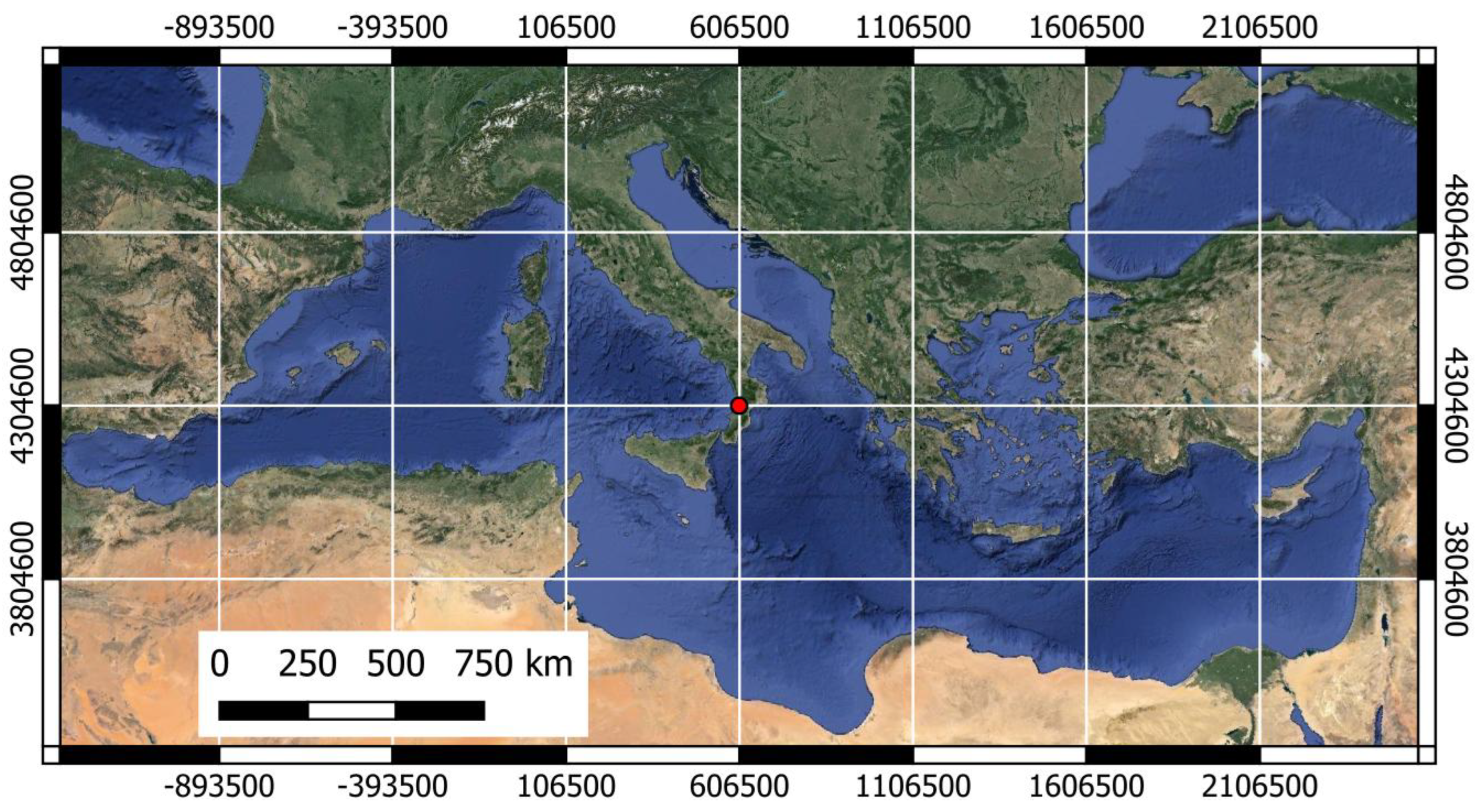
2.1. Site Description

The station of Lamezia Terme (LMT) is operated by the National Research Council of Italy – Institute of Atmospheric Sciences and Climate (CNR-ISAC). The station is a World Meteorological Organization/Regional Global Atmospheric Watch (WMO/GAW) site (38.8763 °N 16.2322 °E, 6 meters above sea level). LMT is a coastal site located 600 m inland from the Tyrrhenian coastline of Calabria (West side, Figure 1). The area is characterized by anthropogenic pollution emissions related to domestic uses, agriculture, transportation, and highway vehicular traffic. Among the key hotspots in the area, Lamezia Terme International Airport (IATA: SUF; ICAO: LICA) (North direction) and the town of Lamezia Terme (North-East direction). The A2 highway runs around the observatory clockwise from North to South and is located 7 km northward to 3.5 km southward from the experimental site. As depicted in Figure 1, the station is close to the Tyrrhenian coast of Calabria, with the island of Sardinia being located 600 kilometers in the W-NW direction. The dominant air masses of synoptic circulation overlap with local breezes, maintaining a strong westerly direction. Looking at the West and South West sectors, there are usually two different occurrences, i.e., one is related to the establishment of breeze regime with winds <5 m/s, characterized by the transport of marine air masses; the other is related to synoptic conditions with winds of more than 9 m/s, occasionally characterized by the transport of ash from the nearby volcanoes Etna, located in mainland Sicily, as well as Vulcano and Stromboli in the Aeolian Islands, or by Saharan-type aerosols (Calidonna et al., 2020; Malacaria et al., 2024). The experimental site is characterized by moderate wind breezes converging on the isthmus of Catanzaro, where the Marcellinara orographic gap links the Tyrrhenian and Ionian seas on a NW-SW sector (see Figure 1), which mainly develop during daytime, while northeastern gentle wind breezes from land mainly affect the night-time period (Federico et al., 2010). Previous research reported the effects of local wind regimes on the daily-to-seasonal variability of methane (D’Amico et al., 2024 https://doi.org/10.3390/atmos15080946) and surface ozone (D’Amico et al., under review; D’Amico et al., 2024 https://doi.org/10.3390/su16188229).

2.2. Experimental

An automatic weather station (Vaisala WXT520, Finland) was used to monitor the following meteorological parameters at 10 m a.g.l.: temperature, relative humidity, wind speed and direction, barometric pressure and rain amount. Instrumental details of the meteorological parameters are given in Table 1.

Since 2015, a Picarro G2401 (California, USA) Cavity Ring Down Spectroscopy (CRDS) analyzer was used to measure CH₄, CO and CO₂ data from ambient air as well as from calibration tanks. The cycling between ambient air and calibration tanks is performed by a 10-way rotative valve (Vici-VALCO model EMTCSD10MWE). The valve sequencer software controls the timing of sample introduction. From the sampling point at a height of approximately 4 m above the ground, ambient air is collected at a rate of 0.260 L min^-1. Starting since February 2022, the air stream is passed through a Nafion dryer (PERMA PURE 1001 model MD-070-72S-4 050420-08) to dry the ambient air. This reduces the residual effect of water vapor on the measurement. The dried air sample is then measured by the CRDS G2401. Prior to this date, we relied on the standard manufacturer's built-in correction functions as reported by Rella et al., (2013) and defined by Chen et al., (2010). According to Rella, (2010), by using these functions, the effects of water vapor on measurements can be corrected with residuals below the WMO targets for water vapor concentrations up to at least 1% and perhaps up to 2%. The application of specific instrument corrections may further allow the WMO targets to be met for an extended range of water vapor values (Zellweger et al., 2016). Unfortunately, no successful attempts were made to determine the instrument-specific water vapor correction factors at LMT. In particular, several attempts were made to perform the test based on the "droplet method" test described in Rella et al., (2013), as well as other in-house developed tests using a Nafion tube to humidify the dry air from a tank (compressed ambient air). Although unfortunate, this is not entirely uncommon: as discussed by Yver-Kwok et al., (2021), it is difficult to perform a good droplet test even when following the standardized ICOS protocols. For these reasons, and to provide an indication of the possible additional uncertainty that may arise due to the lack of implementation of a specific water vapor correction function, we collected the water vapor correction factors available in the literature (Rella et al., 2013; Zellweger et al., 2016; Gomez-Pelaez et al., 2019; Reum et al., 2019), as well as for a G2401 instrument (s/n: CFKADS2269) operated by ISAC and characterized by the ICOS Atmospheric Thematic Center (Yver-Kwok et al., 2021). For a test period (2017-2019), we applied seven different correction factors to the 1-minute wet Picarro G2401 measurements taken at the LMT. We found that, as a function of the different sets of correction factors applied, the mean averaged values of the deviations for CO₂ (CH₄) ranged from less than 0.01 ppm (-0.1 ppb) to 2.5 ppm (9.3 ppb) with respect to the dry mole fractions provided by the instrument, i.e., well above the WMO compatibility goals. Chen et al., (2013) also demonstrated the possibility of obtaining accurate measurements of CO in humid air by using the CRDS technique. Zellweger et al., (2019) argued that due to the relatively large uncertainties of individual experiments and possible changes in the instrument response to water vapor (see also Yver-Kwok et al., 2021), it is not ever feasible to determine a reliable instrument-specific correction function for the CO measurements by near-infrared CRDS instruments like the Picarro G2401. For their specific case, Zellweger et al., (2019) showed that not drying the air sample and using the factory implemented water vapor correction can result in a CO bias of 4.20 ppb with respect to dry measurements. Based on these evidences, it is likely that LMT data for the period prior to February 2022, did not met the WMO compatibility goal for CO.

CH₄, CO and CO₂ data are calibrated against the WMO calibration scales (i.e., CH₄: WMO X2004; CO: WMO X2014 and CO₂: WMO X2019 (Hall et al., 2021)) using a set of three calibration cylinders which are measured (injection time: 30 minutes) during three cycles every 14 days. The calibration cylinders are provided by ESRL's National Oceanic and Atmospheric Administration (NOAA) Global Monitoring Laboratory (GML). These WMO reference gases cover the CO mole fraction from 40 to 500 nmol mol^-1, the CO₂ mole fraction from 250 to 520 µmol mol^-1 and the CH₄ mole fraction from 300 to 2600 nmol mol^-1. In addition to three target cylinders, each with a known concentration of a single gas, are sequentially measured every 19 hours.

CH₄, CO and CO₂ data affected by documented technical problems or equipment maintenance/setup are flagged by LMT operators. The final fully controlled hourly averaged data for the mole fractions of CH₄, CO and CO₂ are obtained by averaging the 1-minute averaged data which, on turn, are obtained from the raw data (5-second time resolution). The hourly, daily and monthly averages of CH₄, CO and CO₂ mole fractions at the Lamezia Terme station reported to national and international databases such as the World Data Centre for Greenhouse Gases (WDCGG) are also based on 1 minute averaged data where local pollution events have been flagged in addition to outliers. Only instrumental and technical problems, but not local pollution events are excluded from the gas datasets. Over the period 2015-2023, the 91.5% of the 1-hour mean values are available for CH₄, CO and CO₂.

2.3. Description of the Models for Background Definition

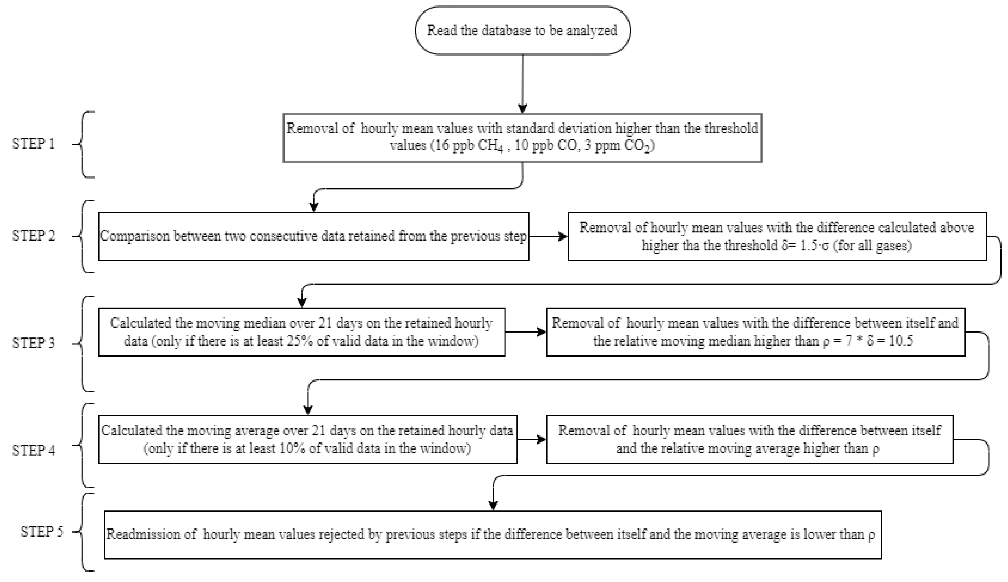
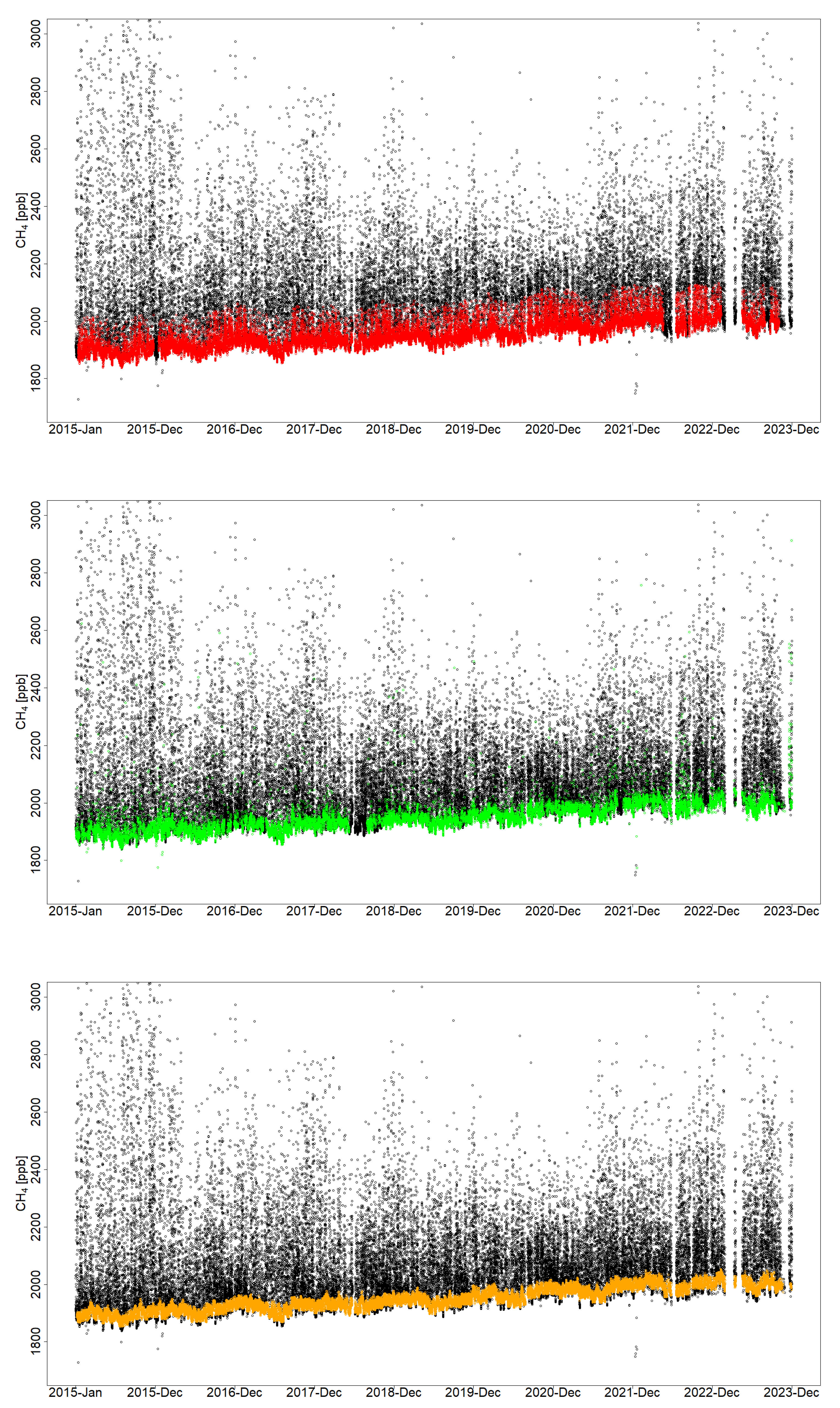
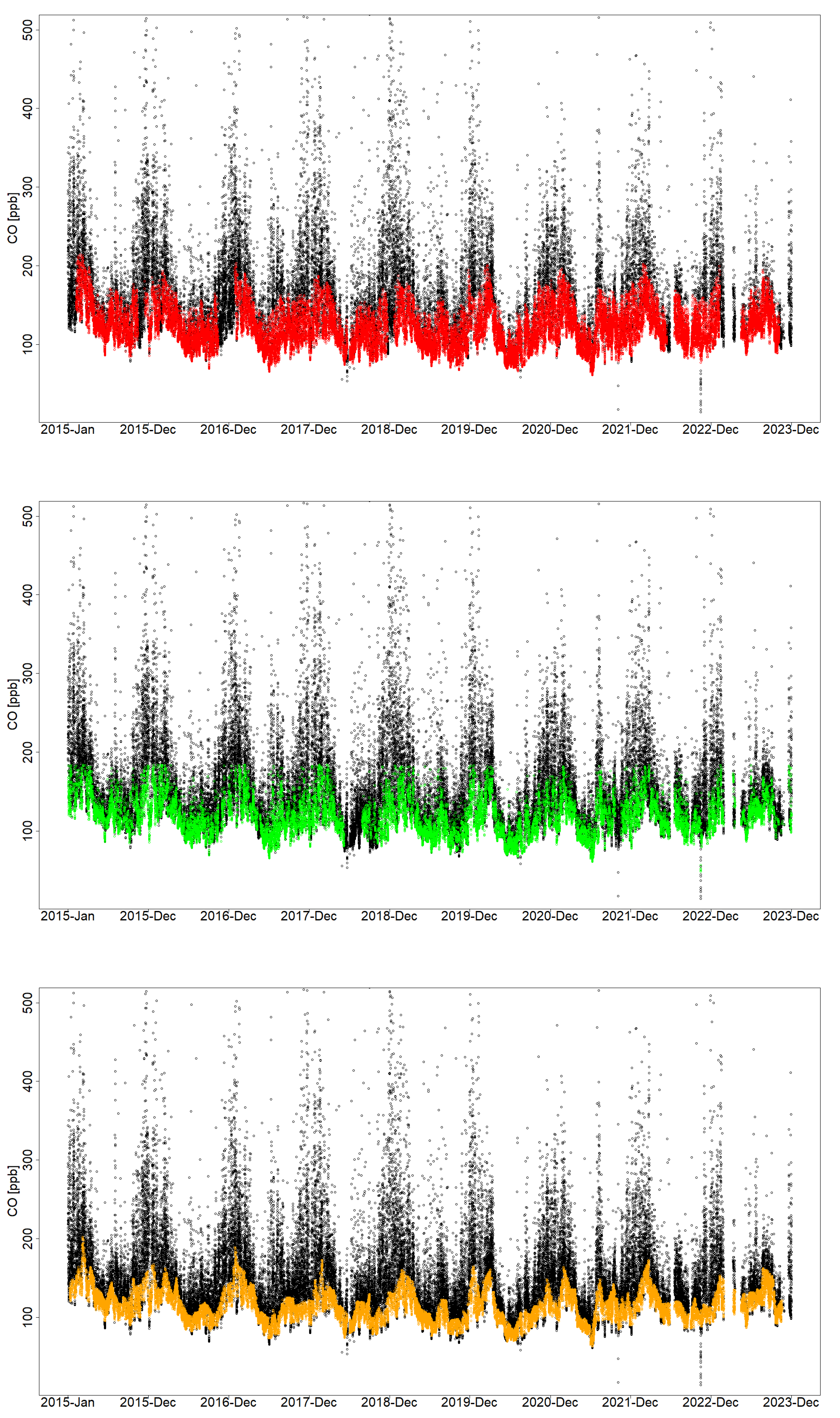
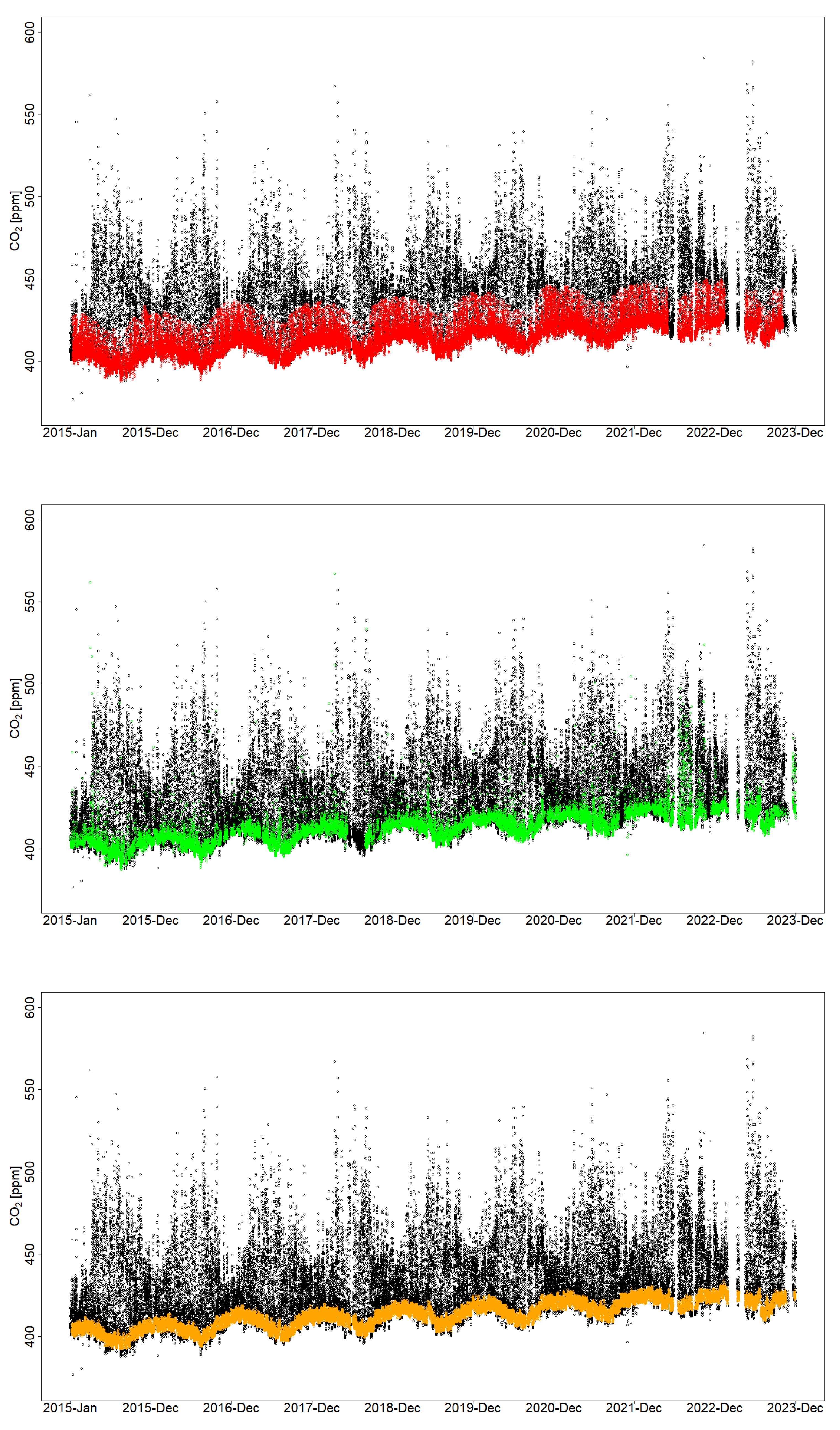
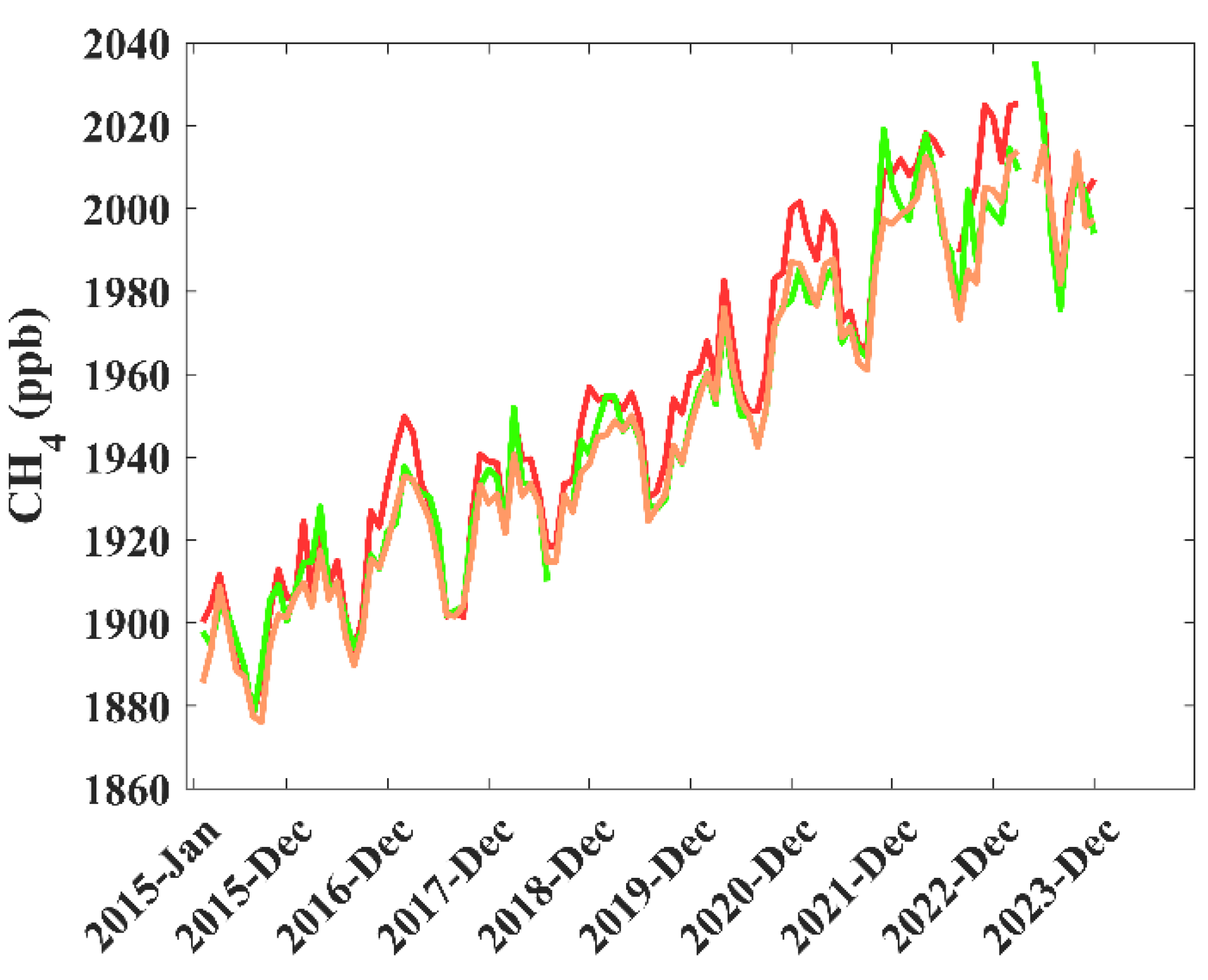
Three different methods were used to select measurement periods representative of the background values for CH₄, CO and CO₂: a statistical method (BaDS-Background Data Selection method), a meteorological method (defined as “Wind”) based on the analysis of wind speed and direction and the smoothed minima (SM) method. The first method (BaDS) is well known and widely used for gas time series, in particular for CO₂ (Trisolino et al., 2021; Apadula et al., 2019); the second method was implemented based on the specific characteristics of the experimental site location and taking into account the meteorological variables, namely wind speed and direction recorded at the LMT station. The third was also used in the literature (Aksoy et al., 2009; Gaoa et al., 2018), but in this work it is implemented with the addition of new steps. We have taken particular care to apply an empirically unbiased identification of the thresholds adopted to identify concentration values of CH₄, CO and CO₂ that well describe the atmospheric background during the study period. A sensitivity study was realized to find the optimal parameters for tuning all the background methods used. This approach allows testing the feasibility of a reasonable view of the background variability of CH₄, CO and CO₂.

2.3.1. BaDS

The BaDS methodology is a statistical method based on the assumption that the GHGs values observed under background conditions are characterized by very little and very slow-paced changes. GHGs sampling resolution time is fixed at 5 seconds, each hour is therefore described by a maximum of 720 values for each gas. Consequently, each hour can be defined as a background if the sub-hourly data characterizing it are similar, i.e., if the derived hourly standard deviation is small. In the same way, if there is little difference between the values for two consecutive hours, we can assume that we are still in background conditions. So the whole method is based on the consideration that a representative background condition is necessarily characterized by a very little variability within the hourly averages and between the couples of two consecutive mean values. Similarly than Trisolino et al., (2020), the threshold values (σ, ρ and δ) were defined after a sensitivity test ran over the complete datasets (72152 hourly data for each of the three gases) so that only plausible background measurements were retained and, at the same time, only a small number of hourly values were removed (37.7% for CH₄, 37.2% for CO and 30.7% for CO₂). Initially, BaDS examined the standard deviation (σ) associated with each hourly mean value: the data point was flagged when σ, calculated from the 1-minute mean values, exceeded a specific given threshold value (16 ppb for CH₄, 10 ppb for CO and 3 ppm for CO₂). Secondly, each data point was compared with the previous one along the time series: it was flagged if the difference exceeded a given threshold δ = 1.5·σ for all gases. Thirdly, a moving median was calculated (time window of 504 hours, i.e., 21 days) over the retained hourly data. The moving median is computed only if there is at least 25% of valid data in the list of the 504 theoretically available hourly data. If the difference between the hourly mean value and the computed median exceeded the threshold ρ = 7·δ = 10.5, the record is flagged as “not-background”. Fourthly, a 504-hours moving average was further applied to the data that passed the previous step (only if there is at least 10% of valid data in the window). If the difference between the hourly mean values and the computed moving average exceeded the threshold value ρ the data point was flagged as “not-background”. Finally, a readmitting procedure was introduced by comparing all the hourly mean values that did not pass the previous steps. If the difference respect to the moving average was lower than ρ, the data point was reintegrated and considered part of the “background” selection.

The flow chart of the described BaDS method is shown in the Figure 2 below.

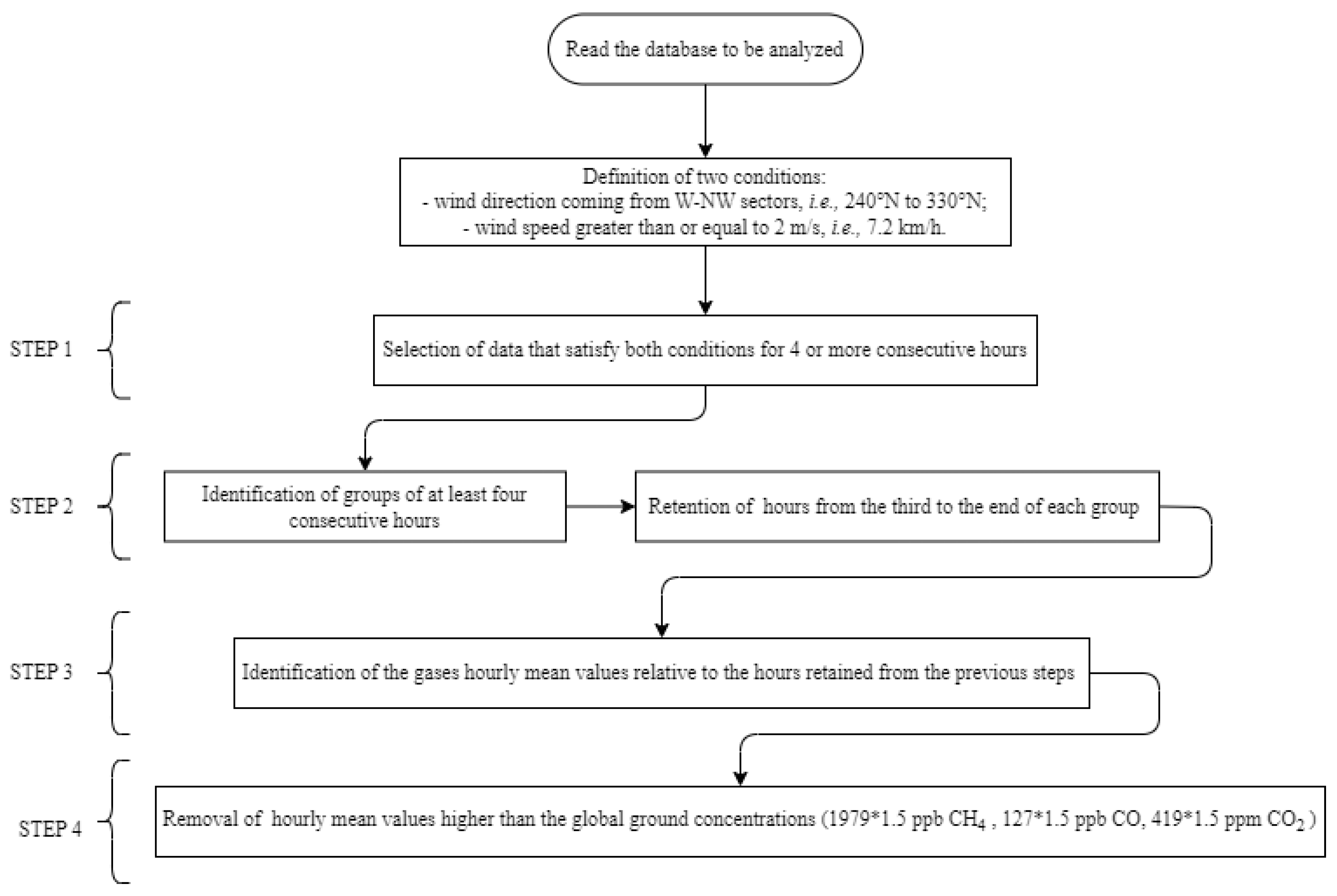
2.3.2. Meteorology-Based Selection

In the second case, a selection method based on the analysis of wind speed and direction observed at LMT was implemented. By this criterion, the local geographical configuration and the positioning of the sampling site with respect to the coastline were both exploited. The experimental site is located approximately 600 m from the Tyrrhenian coastline, with a gas sampling point at 4 meters above the ground. From the observation point, winds have no orographic obstacles up to the southern coast of Sardinia, 600 km in the W-NW sectors (Figure 1). Considering this last one information, it can be plausible to assert that the air masses coming from W-NW sectors are less affected by regional anthropogenic emissions compared to those coming from other directions. Consequently, the method relied on the following criteria to filter data:

- wind direction coming from W-NW sectors, i.e., 240°N to 330°N;

- wind speed greater than or equal to 2 m/s, i.e., 7.2 km/h.

The 2 m/s threshold is defined by considering that the sea breeze regime starts at this wind speed, so in this condition the air masses are coming from the offshore (Malacaria et al., 2024). The selection process retained data that met these requirements for four or more consecutive hours. This condition made it possible to identify groups of at least four hours in which the average wind directions and speeds were persistently attributable to an offshore corridor and presumably less affected by anthropogenic pollution. Therefore, the effects of local recirculation can be expected to be limited under the combination of these conditions. For these selections, only the hourly mean values from the third hour onwards were selected, leaving out the first two hours of each group, as the first part of the selection could be affected by local pollution. In the third step, the hours identified by the previous filter were used to identify the corresponding hourly mean concentrations of CH₄, CO and CO₂. Finally, another filter was applied to remove data exceeding by 1.5 the mean concentration values of 1979 ppb for CH₄, 127 ppb for CO and 419 ppm for CO₂, calculated by averaging the full dataset for each gas. This step is applied because influences of emissions related to marine shipping transportation cannot be completely excluded, which could potentially affect the observed GHGs values. Taking all the selection steps into account, the final data set retained the following percentages of data per species: 35.7% CH₄, 34.7% CO and 35.4% CO₂. A flow chart of the method described above is shown in the following Figure 3.

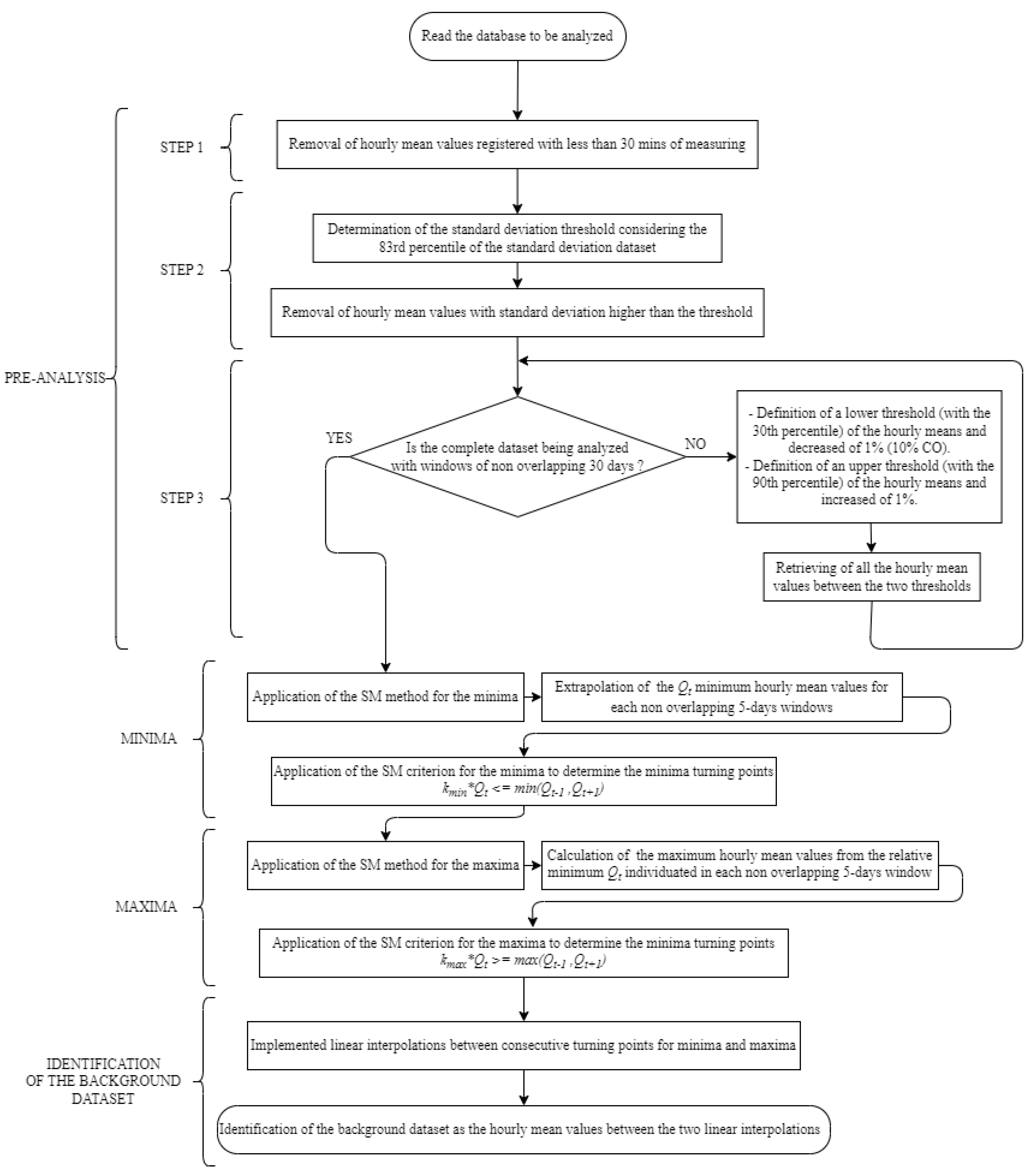
2.3.3. Smoothed Minima (SM)

This method, originally developed for hydrological applications by the United Kingdom Institute of Hydrology (UKIH), was also used to determine the background signal for atmospheric particulate datasets, as reported in the literature (Aksoy et al., 2009; Gaoa et al., 2018). This method removes the sharp peaks and valleys produced by linear interpolation and produces a smoothed signal representing the baseflow generating mechanisms. Therefore, this method has been developed to separate baseflow from total flow by the application of a simple smoothing rule. In this procedure, the time series of hourly mean values were partitioned into equal units of non-overlapping 5-days as proposed in the method presented by Hafzullah Aksoy et al., (2009). For each unit, the minimum value has been determined, obtaining a time series composed of the lowest hourly mean values; mark the minima of each of these units and let them be called Q₁, Q₂, ... Q_t. Consider in turn (Q₁, Q₂, Q₃), (Q₂, Q₃, Q₄), ... , (Q_t-1, Q_t, Q_t+1). In each case if is satisfied, then the central value $Q_t$is a turning point. Continue to identify turning points until the entire time series has been analyzed. In addition, before applying the SM method, an initial analysis was performed to remove all data with excessive negative and positive peaks compared to the typical and known variability of each gas. The analysis includes three consecutive steps: first, all hourly mean values resulting from less than 30 minutes of data were rejected. In a second step, for each gas, the hourly standard deviation values (calculated from the 1-minute average values) were compared with the standard deviation threshold calculated by using the 83^rd percentile of the standard deviation values; the hourly mean values with a standard deviation higher than the standard deviation threshold were also excluded. Regarding the standard deviation threshold, we tested several values and, after analyzing the results, the 83^rd percentile was chosen for each gas, as this allows the selection of a reasonable initial percentage of data to be filtered by the application of the SM method. The thresholds calculated with values lower than the 83^rd percentile may exclude useful data, so the choice of this value is a good compromise. Over a final step, we calculated the 30^th and 90^th percentiles of the hourly mean values over 30-day non-overlapping time windows, obtaining two threshold values. These latter threshold values were both decreased and increased by 1% for CH₄ and CO₂, and decreased and increased by 10% and 1% for CO. We have chosen a 30-day time window to calculate these percentiles (30^th and 90^th) in order to include in the analyzing windows a better distribution of the gases behaviors; the use of smaller windows could produce values that are not well representative of the original datasets, indeed. All hourly mean values between these two thresholds were considered as possible background data and passed to the SM method. We implemented this method by also identifying, for each window (non-overlapping 5-days), a maximum value starting from the respective minimum point, Q_t, increased by the standard deviation threshold calculated as explained above, and subsequently multiplied by a factor p = 1.02 for CH₄, p = 1.15 for CO and p = 1.01 for CO₂. The maximum points were flagged as turning points with a similar criterion shown for the minima:

$$k_{min}*Q_t\le \min \left(Q_{t-1},Q_{t+1}\right)$$

(1)

where:

• $Q_t$ is the central minimum point of the sliding interval;
• $Q_{t-1}$ is the previous minimum point of the same window;
• $Q_{t+1}$ is the next minimum point of the same window;
• $k_{min}$ is a constant value of 0.995, experimentally perfected on the basis of the value reported by Hafzullah Aksoy et al. (2009).

$$k_{max}*Q_t\ge \mathrm{m}\mathrm{a}\mathrm{x}(Q_{t-1},Q_{t+1})$$

(2)

$k_{max}$ is a constant value of 1.01, experimentally selected.

Linear interpolation was implemented between consecutive turning points for minima and maxima. Thus, a baseline for the minima was obtained by connecting all the turning points and by considering the values determined from the linear interpolation, while the upper limit was obtained considering the linear interpolation of the maximum turning points.

All the hourly mean values between the upper and down limit lines are considered as background data. The application of the SM extended method led to a final dataset including, compared to the initial datum, 51.0% of CH₄, 43.1 % of CO and 49.3% of CO₂ measurements. A flow chart of the SM method described can be seen in the Figure 4 below.

The methods described in this section of the paper have been applied to the entire time series available at LMT.

2.4. Adopted Metrics for Calculating Temporal Tendencies

With the purpose of investigating and quantify the 9-year tendencies that characterize LMT time series, we used distributed, Mann-Kendall (Gilbert, 1987; Helsel and Hirsch, 1993; Mann, 1945; Kendall, 1975) and Sen's slope estimator (Şen, 2012). We adopted these descriptors to detect the presence of tendency and quantify and slopes because the hourly mean data of CH₄, CO and CO₂ at LMT were not normally distributed. Therefore, the presence of a monotonic increasing or decreasing tendency was examined using the non-parametric Mann-Kendall test and the slope of a linear tendency was estimated using the non-parametric Sen’s method. Even if the tendencies are in the same direction, applying the Mann-Kendall test to each month can still reveal temporal processes that would not otherwise be detectable using – for example – the seasonal Mann-Kendall test. In this study, the Mann-Kendall test was applied separately for each season on a per-year basis. Selected datasets were therefore reduced, which may affect whether or not a statistically significant tendency can be noticed, but if the results are indeed significant, it may help understand what is driving these changes.

The Mann-Kendall test is deemed suitable in circumstances where the observed tendency can be assumed to be monotonic, with no evidence of a cyclic pattern such as a seasonal change over the course of a year. Obviously, this is not the case for the atmospheric tracers considered in this work. Thus, it should be clearly stated that the application of a linear tendency descriptor not strictly imply the assumption of a linear tendency in the analyzed time series (Crimmins, 2020). Sen's method used a linear model to estimate the slope of the tendency and the variance of the residuals, the last one should be constant over time. Overall, both methods have clear advantages such as the handling of missing data, the need for few assumptions and independence of the data distribution (Öztopal and Sen, 2017; Wu and Qian, 2017; Kisi, 2015) that made them suitable for atmospheric data analysis. Missing values were allowed, and the data did not have to follow any particular distribution. In addition, Sen's method was not significantly affected by single data errors or outliers. The number of years in the data series examined for each gas was denoted by n. Missing values were allowed and n can therefore be less than the number of years in the series under consideration.

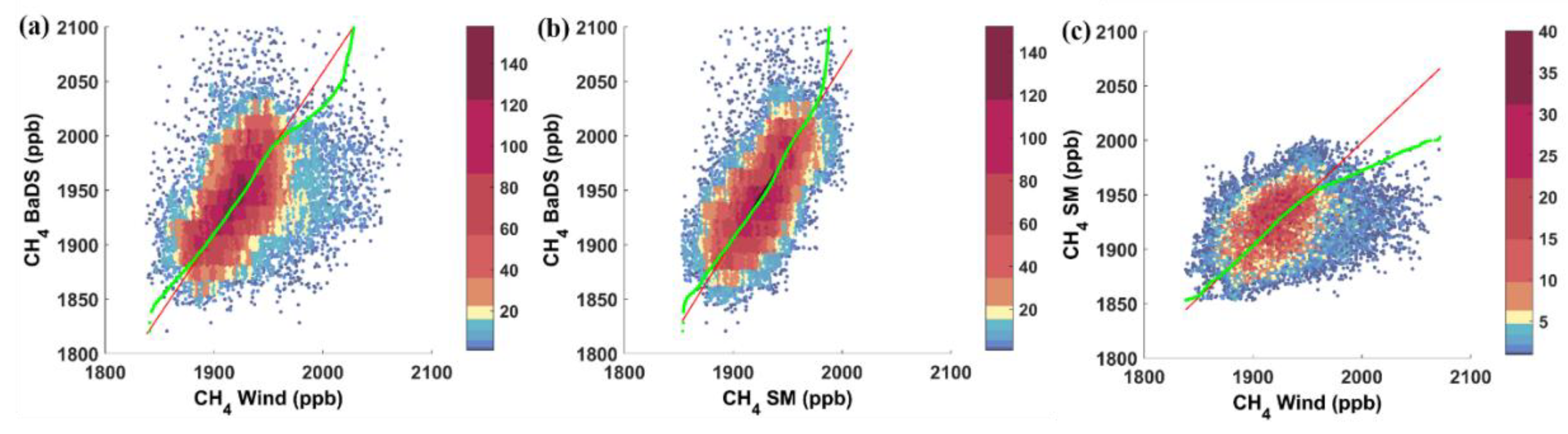
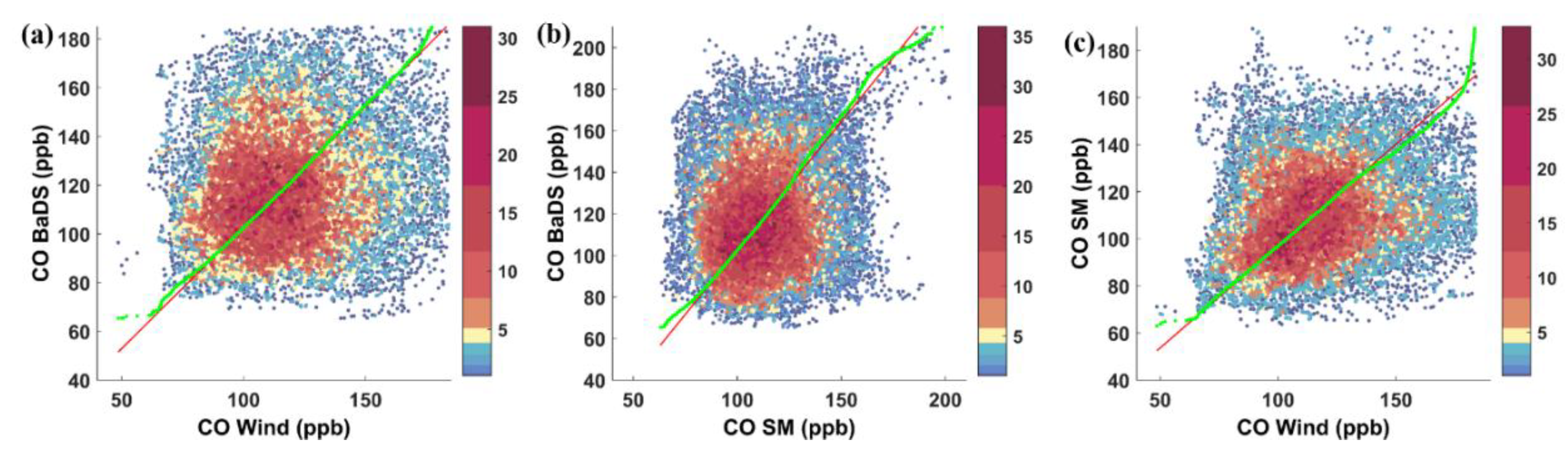
2.4.1. Adopted Metrics to Compare Background Selection Methods

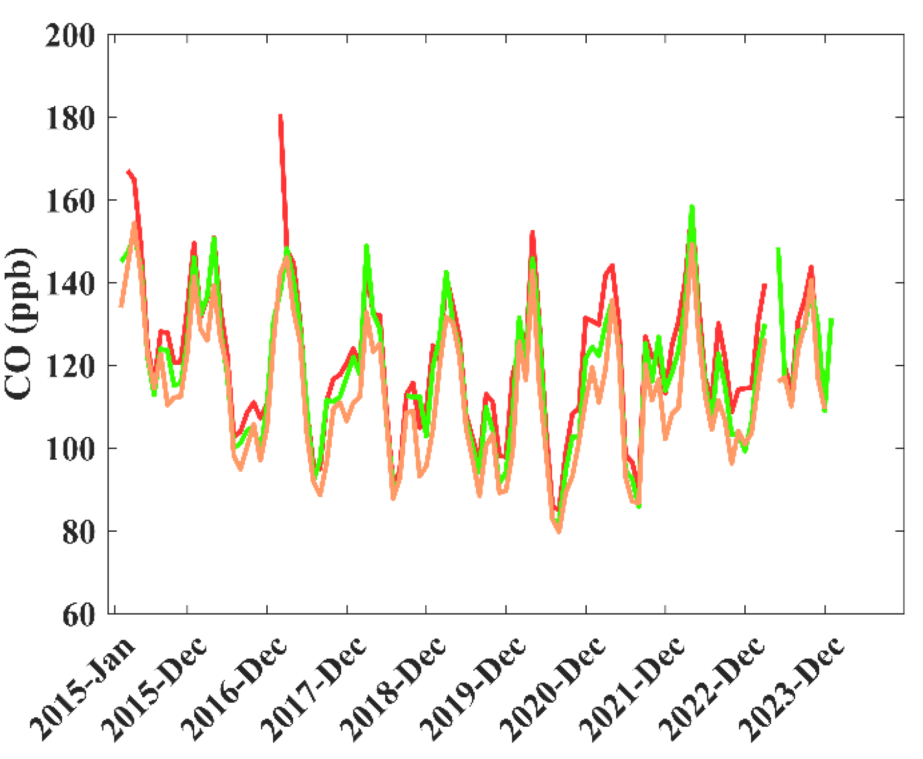
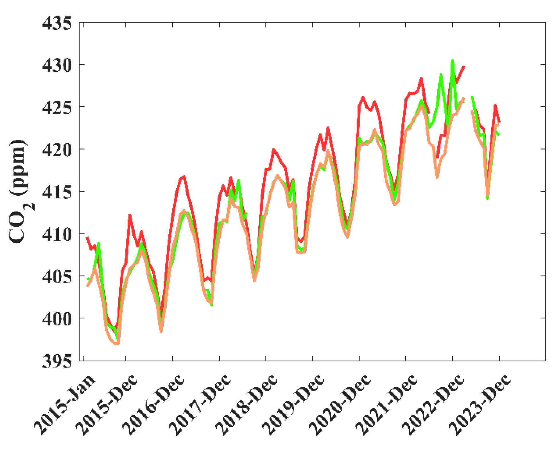
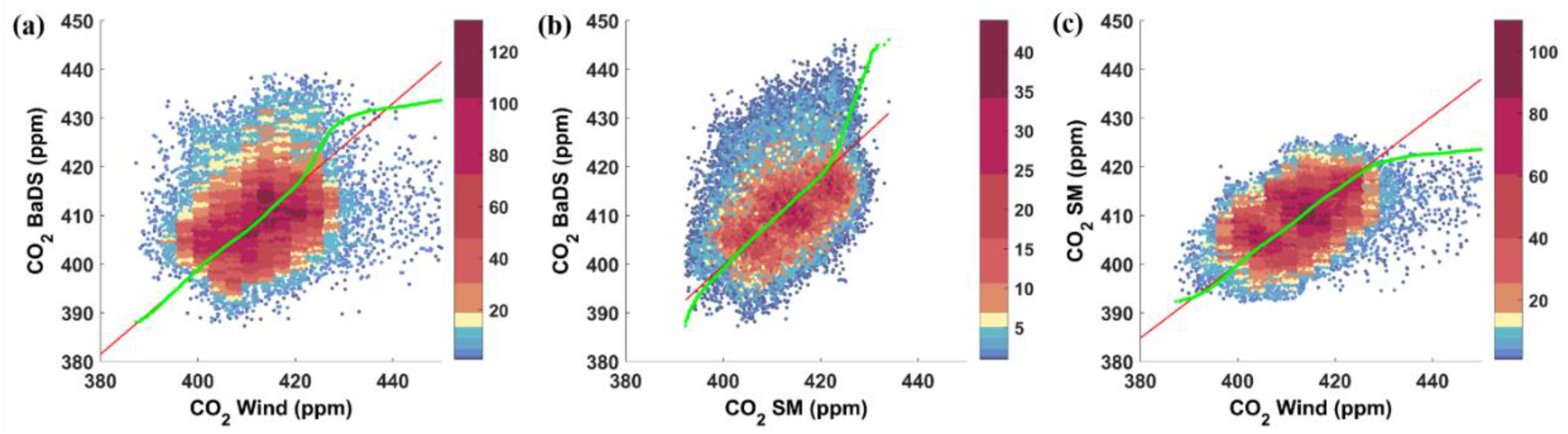
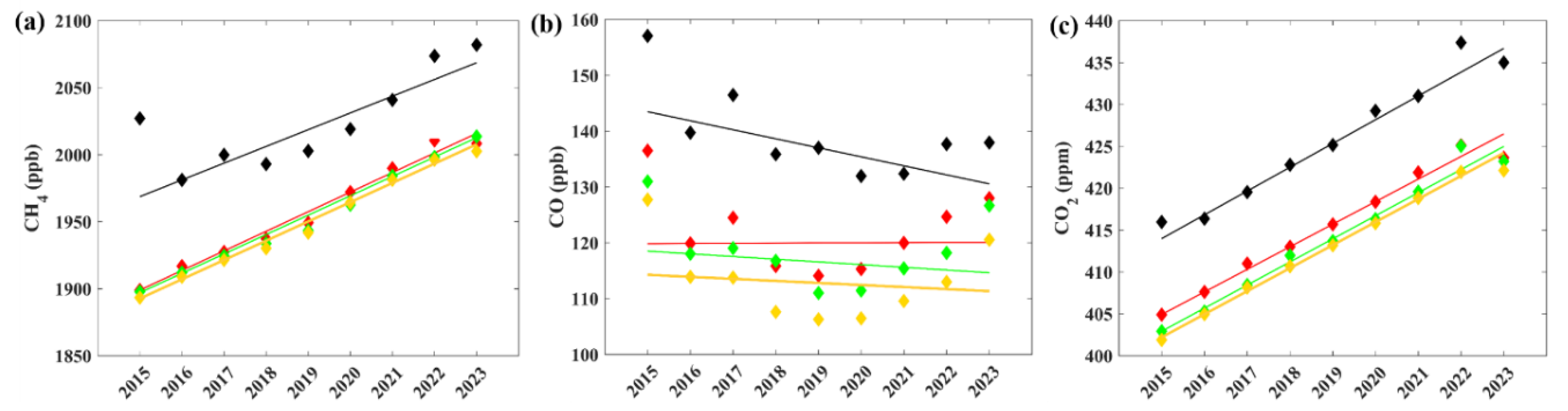
In this work we used the error metrics defined as the Root Mean Square Error, RMSE (Equation 3), the arithmetic mean value of the errors, Bias (Equation 4), the Scatter Index, SI (Equation 5) that is a normalized measure of error reported as a percentage, and the correlation coefficient, R² (Equation 6). Lower values of the SI are an indication of better model performance. A negative BIAS represents an underestimation of the x-axis dataset relative to the y-axis dataset.

$$\mathrm{RMSE}=\sqrt{{\displaystyle \frac{{\sum }_{\mathrm{i}}({\mathrm{e}}_{\mathrm{i}}-{\mathrm{o}}_{\mathrm{i}}{)}^2}{\mathrm{n}}}}$$

(3)

$$\mathrm{BIAS}={\displaystyle \frac{{\sum }_{\mathrm{i}}\left({\mathrm{e}}_{\mathrm{i}}-{\mathrm{o}}_{\mathrm{i}}\right)}{\mathrm{n}}}$$

(4)

$$\mathrm{SI}={\displaystyle \frac{ \mathrm{RMSE}}{\stackrel{\mathrm{-}}{\mathrm{o}}}}$$

(5)

$${\mathrm{R}}^2=({\displaystyle \frac{cov\left(o_i ,e_i \right)}{\mathrm{stdv}{o}_i*\mathrm{stdv}{e}_i}}$$

(6)

In all formulations, e_i is the estimation of a certain variable, o_i represents the other sample of dataset, n is the amount of data, stdv is the standard deviation, and cov is the covariance.

3. Results

The LMT coastal station has allowed continuous monitoring of CH₄, CO and CO₂ mole fractions in a region characterized by Mediterranean climate. Three methodologies described in section 2.3 have been applied to extract background data from the time series of atmospheric gases in order to identify measurements deemed well representative of atmospheric background levels. In Figs. 5, 6, and 7 we report the selection of the background data obtained from the application of the BaDS, Wind and SM methods to the complete datasets (black dots) for each gas. The BaDS method selected the following percentages as background data: 62.3% for CH₄; 62.7% for CO; 69.3% for CO₂. Data percentages 35.7% and 51.0% for CH₄, 34.7% and 43.1% for CO, 35.4% and 49.3% for CO₂ were filtered even further via cut-off parameters of Wind and SM methods for each gas (Figure 5, Figure 6 and Figure 7).

Figure 8, Figure 9 and Figure 10 show the CH₄, CO and CO₂ time series respectively, reporting monthly mean values over the 2015-2023 period using the three background methodologies described before. The variability of the monthly mean values is more regular for CH₄ and CO₂ (Figs. 8 and 10) than for CO (Figure 9), with a marked seasonality and a constant increase over the years. In general, BaDS (SM) recorded the highest (lowest) values for all the gases considered, with values differing up to tenths of ppb for CH₄ and CO and a few ppm for CO₂ for specific months depending on the method considered.

A comparison between the three background methods was performed using the error metrics described in section 2.4.1 and visualizing both the scatter and q-q plots (quantiles of sample data x-axis versus quantiles of sample data y-axis) based to the hourly mean values of CH₄, CO and CO₂ background datasets (Figure 11, Figure 12 and Figure 13, respectively). For each of these last figures mentioned, q-q plots report these comparisons as follows: BaDS (y-axis) and Wind (x-axis) (a); BaDS and SM (b); SM and Wind (c). Green lines represent quantile–quantile plots and red lines mark least-square best fits. If the compared methods select the same data, the green lines of the q-q plot would be linear, which would coincide with the least squares best fit shown by a red line.

The error metrics used for BaDS, Wind and SM background datasets of CH₄, CO and CO₂ in the entire 2015-2023 period are shown in Table 2. In detail, the statistical parameters are the Root Mean Square Error (RMSE) (Equation 3), the arithmetic mean value of the errors (BIAS) (Equation 4), the Scatter Index (SI) (Equation 5), and the correlation coefficient (R²) (Equation 6).

For the observed gases, the highest RMSE values are shown in the BaDS-Wind comparison. For CH₄ and CO, the comparison between the BaDS-SM and BaDS-Wind datasets highlights positive BIAS values, indicating an overestimation of BaDS values relative to the SM and Wind datasets. By the other hand, the comparison between the SM and Wind datasets results in a negative BIAS value, indicating an underestimation of background values defined by Wind relative to SM. For CO₂, BIAS values are negative for all three comparisons of the background method datasets. Therefore, the Wind method results into underestimations compared to the BaDS and SM datasets, while the comparison between the BaDS and SM datasets results in underestimated values compared to the BaDS dataset. Regarding the R² values obtained following the comparisons between the three background datasets, no high correlations are found as the values are below 0.4. For CH₄ and CO₂ the best performances with 2-3% SI values have been obtained, that considering all analyzed comparisons.

The adoption of the different background selection methods to the identification and quantification of gases tendencies in the 9-years at LMT were investigated by computing non-parametric Mann-Kendall test (Gilbert, 1987; Helsel and Hirsch, 1993; Mann, 1945; Kendall, 1975) and Sen’s slope estimator (Şen, 2012) on a monthly basis (Table 3, Table 4, Table 5 and Table 6, and Figure 14). Please note that the application of monotonic or linear tendency descriptor (like Mann-Kendall test and Sen’s slope) does not imply the assumption of the existence of linear or monotonic tendency (in the case of CO) in the analyzed data.

Particularly, Table 3, Table 4, Table 5 and Table 6 show the number of years in the data series examined for each gas n, the Mann-Kendall test statistic S (test S, Equation S1) that has been used to identify possible monotonic increasing or decreasing tendencies, the levels of significance, and the A (slope) and B (intercept) coefficients as defined in Equation S5. Tables show seasonal and annual mean values calculated starting from hourly mean values. Seasons are divided as follows: winter (December, January, February – DJF), spring (March, April, May – MAM), summer (June, July, August – JJA) and fall (September, October, November – SON). Monthly mean values over the 2015-2023 period, calculated starting from hourly mean values, of gases are shown in the Supplementary Material; in particular, in Table S1 the complete hourly mean datasets of CH₄, CO and CO₂ are reported.

Tables S2, S3 and S4 show the monthly mean background values of CH₄, CO and CO₂ respectively.

In Table 3, both the non-parametric Mann-Kendall test and Sen’s method were applied to the complete hourly mean datasets of CH₄, CO and CO₂. In Table 4, Table 5 and Table 6 tendency methodologies were applied to hourly mean value datasets of CH₄, CO and CO₂, respectively, selected by BaDS, Smoothed minima, SM and Wind background methods, over the entire 2015-2023 period.

As described in section “methods” in the Supplementary Material, we have calculated four different levels of significance α. When analyzing the complete dataset for CO₂, we observe the maximum level of significance for the majority of months (Tab. S1), seasons and annual values (Tab. 3), except for the months of April, August and November, which show lower levels of significance. For CH₄ as a whole, the dominant level of significance is α = 0.05 for all months (Tab. S1), seasons and years (Tab. 3). The application of Mann-Kendall’s test to the three background datasets for CH₄ (Tab. 4 and Tab. S2) and CO₂ (Tab. 6 and Tab. S4) show the maximum levels of significance (*** α = 0.001) for all periods considered in the tables. For CO, no statistically significant tendencies were observed neither for the original dataset (Tab. 3 and Tab. S1), not for the three background datasets (Tab. 5 and Tab. S3).

For each gas analyzed over the observation period, Figure 14 reports in detail CH₄ (a), CO (b) and CO₂ (c) results related to the application of non-parametric Sen's method to annual mean values for complete datasets (black linear tendency), BaDS (red linear tendency), Wind (green linear tendency) and SM (orange linear tendency) background datasets. Despite our findings show a considerable annual variability of CH₄, CO and CO₂, the results allowed to infer a strong positive tendency for CH₄ (a) and CO₂ (c), while CO (b) shows a slightly negative tendency possibly mimicking the decrease of CO anthropogenic emissions in Europe (Fortems-Cheiney et al., 2024). The application of the three selection methods had a clear impact on the quantification of multi-annual tendencies compared to the original dataset. For example, looking at the annual growth rates (as derived from the Sen's slope reported in Tables 3 - 6), higher (lower) values were obtained for CH₄ (CO₂) and the statistical significance of the detected tendencies increased for CH₄. However, not negligible differences between the different methods can be observed: for the different seasonal aggregations, deviations up to 1.5 ppb/yr, 1.2 ppb/yr and 0.4 ppm/yr characterize the three background datasets for CH₄, CO and CO₂, respectively.

4. Discussion

In order to identify measurements deemed well representative of the atmospheric background, we report in Figure 5, Figure 6 and Figure 7 the selection of background data obtained by applying the BaDS, Wind and SM methods to the complete datasets (black dots) for CH₄, CO and CO₂, respectively.

For each gas the Wind method has a higher percentage of rejected data than the other two methods, specifically 64.3% for CH₄, 65.3% for CO and 64.6% for CO₂ (Figure 5, Figure 6 and Figure 7), indicating that this method provided the strictest data selection for background conditions (35.7% for CH₄, 34.7% for CO and 35.4% for CO₂). The CH₄, CO and CO₂ time series of the datasets selected using the three background methods are shown in Figure 8, Figure 9 and Figure 10, respectively; monthly mean values within the 2015-2023 period are hereby reported.

The seasonal variations of CH₄, CO and CO₂ through the years are prominent, with maxima in the first months of each year and minima during summer seasons, in general agreement with observations across ICOS (Integrated Carbon Observation System) stations in Europe (https://www.icos-cp.eu/observations/station-network, accessed on June 2024). It is worth noting that while multi-year tendencies of well-mixed GHGs CH₄ (Figure 8) and CO₂ (Figure 10) are upward, CO (Figure 9) reported a decreasing tendency. The reduction in CO levels is consistent with the effects of national and international regulations focused primarily on climate change mitigation across Europe, the USA, and China in the past two decades (Gialesakis et al., 2023; Zheng et al., 2018). The annual growth rate in CH₄ at LMT is generally in line with global measurements by NOAA (Hall et al., 2021), (https://gml.noaa.gov/ccgg/trends_ch4/, accessed on June 2024). A previous study performed at LMT reported an average 135.9-139.9 ppb difference between LMT and NOAA annual means with respect to the 2016-2022 period, and an observed peak of 150.1 ppb in 2017 (D’Amico et al., 2024 https://doi.org/10.3390/atmos15080946). The same study reported a surge of CH₄ levels in 2020 and 2021, years well known to be deeply affected by the Covid-19 outbreak. This is in accordance with an increase of CH₄ concentrations observed on a global scale (Lan et al., 2024; Laughner et al., 2021; McNorton et al., 2022; Peng et al., 2022). For CO₂, there is a well-defined multi-year increasing tendency, in accordance with literature (Trisolino et al., 2021) and, https://gml.noaa.gov/ccgg/trends/, accessed on June 2024. The seasonal CO₂ cycle was a combination of different contributions such as atmospheric transport, removal processes, biosphere emissions, as well as fires from agricultural residues (Malacaria et al., 2024) and anthropogenic emissions on different temporal and spatial scales.

The application of the three selection methods affected in a not completely negligible way the mean monthly values of the considered trace gases as well as the calculation of the multi-annual tendencies.

To compare the three background methods applied to the original datasets of gases, in Figure 11, Figure 12 and Figure 13 we report the error metrics described in Section 2.4.1 to visualize the dispersion of q-q plots referred to hourly mean values of CH₄, CO and CO₂ background datasets, respectively.

For CH₄, the quantile-quantile regression among the three different background selection methods showed a linear relationship (Figure 11) coincide with the least-square best fits in the 1850-1950 ppb range, where the highest number of measured data are located (red in bar colors). For CH₄ values higher than 1950 ppb, a drift is observed in all the three comparisons: this was attributed to the low density of available data. Furthermore, the quantile-quantile regression for CO and CO₂ reported a linear behavior (Figure 12 and 13, respectively): only for CO (CO₂) values higher than 190 ppb (420 ppm) a drift is observed with respect to the least-square best fits.

Quantile-quantile plots provide a useful way to study the distribution analysis of gases background datasets. By comparing the integrals of two probability density functions in a single plot, q-q plotting methods were able to capture the location, scale, and skew of a dataset. These comparisons between background datasets of CH₄, CO and CO₂ suggest that the three methods allow to obtain comparable results. Depending on the inherent characteristics of each background selection method, the Wind method is a more stringent method for identifying background data because it is based on two necessary and sufficient conditions that are met simultaneously. For the BaDS and SM methods, the percentages of background datasets for each gas are similar. Among the advantages of applying the three background identification methods to the experimental gas datasets at LMT, we emphasize that the selection results by the three methods are independent of the length of the dataset, which may also consist of only one year of hourly mean data.

5. Conclusions

Our work documents the identification of background data using well-known statistical methods from literature and the potential impacts of adopting these different background selection methods to the identification and quantification of multi-annual tendency in atmospheric GHGs mole fraction at the Lamezia Terme WMO/GAW station (Southern Italy). The key findings in this research will be useful to increase existing information regarding the analysis of CH₄, CO, and CO₂ variability in the Mediterranean basin.

Here we present the complete datasets of CH₄, CO and CO₂ as detected at the LMT WMO/GAW station observed over nine years (2015-2023). In order to discriminate CH₄, CO and CO₂ observations as representative and non-representative of atmospheric background conditions at LMT, we implemented the methodology presented in Apadula et al., 2019 (BaDS), a criterion based on meteorological analysis obtained by evaluating the atmospheric mechanisms and air masses transport processes to the experimental site (Wind) and finally, the smoothed minima methodology (SM) (Aksoy et al., 2009; Gaoa et al., 2018).

The tested algorithms are efficient in the identification of the background data, as suggested by the decrease in absolute values and temporal variability of the considered trace gases after their application. The advantages of the methods are mainly in their versatility and ease of reproducibility. The “Wind” selection method appeared to be the most restrictive criterion, selecting about half of the data selected by the BaDS method. The nonparametric Mann-Kendall test and Sen’s slop estimator were used to investigate the tendencies in CH₄, CO and CO₂ between 2015 and 2023 for the original dataset and for the different subsets resulting from the application of the three background selection methods. For the original dataset, the results show seasonal and annual increasing tendencies for CH₄ and CO₂ with a significance levels of α = 0.05 and α = 0.001, respectively. Regarding CO, a decreasing tendency was only observed for the winter season (α = 0.05). The application of the three selection methods led to a different quantification of the multiannual tendencies and their robustness, as deduced from the analysis of the associated statistical significances. Non-negligible deviations were also found for the average annual growth rates calculated for the three background datasets: for CO₂, for example, the seasonal growth rates changed by more than 0.3 ppm/yr as a function of the different background selections. This suggests that the choice of background selection method may partially influence the quantification of annual growth rates. It is recommended that more than one background selection method is used to quantify the potential uncertainty associated with the method application. Further efforts will be pursued to assess the application of the discussed methods to observations carried out at measurement sites with different environmental conditions.

References

1. Aksoy, H. , Kurt, I., Eris, E. Filtered smoothed minima baseflow separation method. Journal of Hydrology 2009, 372, 94–101. [Google Scholar] [CrossRef]
2. Alexe, M. , Bergamaschi, P., Segers, A., Detmers, R., Butz, A., Hasekamp, O., Guerlet, S., Parker, R., Boesch, H., Frankenberg, C., et al. Inverse modelling of CH4 emissions for 2010–2011 using different satellite retrieval products from GOSAT and SCIAMACHY. Atmos. Chem. Phys 2015, 15, 113–133. [Google Scholar] [CrossRef]
3. Andrews, A.E. , Kofler, J.D., Trudeau, M.E., Williams, J.C., Neff, D.H., Masarie, K.A., Chao, D.Y., Kitzis, D.R., Novelli, P.C., Zhao, C.L., Dlugokencky, E.J., Lang, P.M., Crotwell, M.J., Fischer, M.L., Parker, M.J., Lee, J.T., Baumann, D.D., Desai, A.R., Stanier, C.O., De Wekker, S.F.J., Wolfe, D.E., Munger, J.W., Tans, P.P. CO2, CO, and CH4 measurements from tall towers in the NOAA Earth System Research Laboratory’s Global Greenhouse Gas Reference Network: instrumentation, uncertainty analysis, and recommendations for future high-accuracy greenhouse gas monitoring efforts. Atmos. Meas. Tech 2014, 7, 647–687. [Google Scholar] [CrossRef]
4. Apadula, F. , Cassardo, C., Ferrarese, S., Heltai, D., Lanza, A. Thirty Years of Atmospheric CO2 Observations at the Plateau Rosa Station, Italy. Atmosphere 2019, 10, 418. [Google Scholar] [CrossRef]
5. Artuso, F. , Chamard, P., Piacentino, S., Sferlazzo, D.M., De Silvestri, L., Di Sarra, A., Meloni, D., Monteleone, F. Influence of transport and trends in atmospheric CO2 at Lampedusa. Atmos. Environ 2009, 43, 3044–3051. [Google Scholar] [CrossRef]
6. Balzani Lo¨o¨v, J.M. , Henne, S., Legreid, G., Staehelin, J., Reimann, S., Pre´voˆt, A.S.H., Steinbacher, M., Vollmer, M.K. Estimation of background concentrations of trace gases at the Swiss Alpine site Jungfraujoch (3580 m asl). Journal of Geophysical Research 2008, 113, D22305. [Google Scholar] [CrossRef]
7. Bergamaschi, P. , Houweling, S., Segers, A., Krol, M., Frankenberg, C., Scheepmaker, R.A., Dlugokencky, E., Wofsy, S.C., Kort, E.A., Sweeney, C., et al. Atmospheric CH4 in the first decade of the 21st century: Inverse modeling analysis using SCIAMACHY satellite retrievals and NOAA surface measurements. J. Geophys. Res. Atmos 2013, 118, 7350–7369. [Google Scholar] [CrossRef]
8. Calidonna, C.R. , et al. Five years of dust episodes at the Southern Italy GAW Regional Coastal Mediterranean Observatory: Multisensors and modeling analysis. Atmosphere 2020, 11, 456. [Google Scholar] [CrossRef]
9. Carpenter, L. , Green, T., Mills, G., Bauguitte, S., Penkett, S., Zanis, P., Schuepbach, E., Schmidbauer, N., Monks, P., Zellweger, C. Oxidized nitrogen and ozone production efficiencies in the springtime free troposphere over the Alps. J. Geophys. Res 2000, 105, 14547–14559. [Google Scholar] [CrossRef]
10. Chen, H. , Winderlich, J., Gerbig, C., Hoefer, A., Rella, C. W., Crosson, E. R., Van Pelt, A. D., Steinbach, J., Kolle, O., Beck, V., Daube, B.C., Gottlieb, E. W., Chow, V. Y., Santoni, G. W., and Wofsy, S. C. High-accuracy continuous airborne measurements of greenhouse gases (CO2 and CH4) using the cavity ringdown spectroscopy (CRDS) technique. Atmos. Meas. Tech 2010, 3, 375–386. [Google Scholar] [CrossRef]
11. Chen, H. , Karion, A., Rella, C. W., Winderlich, J., Gerbig, C., Filges, A. Accurate measurements of carbon monoxide in humid air using the cavity ring-down spectroscopy (crds) technique. Atmospheric Measurement Techniques 2013, 6, 1031–1040. [Google Scholar] [CrossRef]
12. Crimmins, A. Improving the use of calibrated language in US climate assessments. Earth’s Future 2020, 8, e2020EF001817. [Google Scholar] [CrossRef]
13. Cristofanelli, P. , Busetto, M., Calzolari, F., Ammoscato, I., Gullì, D., Dinoi, A., Calidonna, C.R., Contini, D., Sferlazzo, D., Di Iorio, T., Piacentino, S., Marinoni, A., Maione, M., Bonasoni, P. Investigation of reactive gases and methane variability in the coastal boundary layer of the central Mediterranean basin. Elem. Sci. Anth 2017, 5, 1–21. [Google Scholar] [CrossRef]
14. Cundari, V. , Colombo, T., Ciattaglia, L. Thirteen years of atmospheric carbon dioxide measurements at Mt. Cimone station, Italy. Il Nuovo Cim. C 1995, 18, 33–47. [Google Scholar] [CrossRef]
15. Curcoll, R. , Camarero, L., Bacardit, M., Agueda, A., Grossi, C., Gacia, E., Font, A., Morguí, J.-A. Atmospheric carbon dioxide variability at Aigüestortes, central Pyrenees, Spain. Reg. Environ. Change 2019, 19, 313–324. [Google Scholar] [CrossRef]
16. D’Amico, F. , Ammoscato, I., Gullì, D., Avolio, E., Lo Feudo, T., De Pino, M., Cristofanelli, P., Malacaria, L., Parise, D., Sinopoli, S., De Benedetto, G., Calidonna, C.R. Integrated Analysis of Methane Cycles and Trends at the WMO/GAW Station of Lamezia Terme (Calabria, Southern Italy). Atmosphere 2024, 2024071587. [Google Scholar] [CrossRef]
17. D’Amico, F. , Gullì, D., Lo Feudo, T., Ammoscato, I., Avolio, E., De Pino, M., Cristofanelli, P., Busetto, M., Malacaria, L., Parise, D., Sinopoli, S., De Benedetto, G., Calidonna, C.R. Cyclic and multi-year characterization of surface ozone at the WMO/GAW coastal station of Lamezia Terme (Calabria, Southern Italy): implications for the local environment, cultural heritage, and human health. Environments 2024, 11, 227. [Google Scholar] [CrossRef]
18. D’Amico, F. , Ammoscato, I., Gullì, D., Avolio, E., Lo Feudo, T., De Pino, M., Cristofanelli, P., Malacaria, L., Parise, D., Sinopoli, S., De Benedetto, G., Calidonna, C.R. Trends in CO, CO2, CH4, BC, and NOx during the First 2020 COVID-19 Lockdown: Source Insights from the WMO/GAW Station of Lamezia Terme (Calabria, Southern Italy). Atmosphere 2024, 2024071587. [Google Scholar] [CrossRef]
19. Derwent, R. , Simmonds, P., O’Doherty, S., Ciais, P., Ryall, D. European source strengths and northern hemisphere baseline concentrations of radiatively active trace gases at Mace Head, Ireland. Atmos. Environ 1998, 32, 3703–3715. [Google Scholar] [CrossRef]
20. Edwards, D.P. , et al. Observations of carbon monoxide and aerosols from the Terra satellite: Northern Hemisphere variability. Journal of geophysical research 2004, 109, D24202. [Google Scholar] [CrossRef]
21. Federico, S. , Pasqualoni, L., Sempreviva, A.M., De Leo, L., Avolio, E., Calidonna, C.R., Bellecci, C. The seasonal characteristics of the breeze circulation at a coastal Mediterranean site in South Italy. Adv. Sci. Res 2010, 4, 47–56. [Google Scholar] [CrossRef]
22. Forrer, J. , Rüttimann, R., Schneiter, D., Fischer, A., Buchmann, B., Hofer, P. Variability of trace gases at the high-Alpine site Jungfraujoch caused by meteorological transport processes. J. Geophys. Res 2000, 105, 12241–12251. [Google Scholar] [CrossRef]
23. Fortems-Cheiney, A. , Broquet, G., Potier, E., Plauchu, R., Berchet, A., Pison, I., Denier van der Gon, H., Dellaert, S. CO anthropogenic emissions in Europe from 2011 to 2021: insights from Measurement of Pollution in the Troposphere (MOPITT) satellite data. Atmos. Chem. Phys 2024, 24, 4635–4649. [Google Scholar] [CrossRef]
24. Frey, M. , Sha, M.K., Hase, F., Kiel, M., Blumenstock, T., Harig, R., Surawicz, G., Deutscher, N.M., Shiomi, K., Franklin, J.E., et al. Building the Collaborative Carbon Column Observing Network (COCCON): Long-term stability and ensemble performance of the EM27/SUN Fourier transform spectrometer. Atmos. Meas. Tech 2019, 12, 1513–1530. [Google Scholar] [CrossRef]
25. Friedlingstein, P. , O'sullivan, M., Jones, M.W., Andrew, R.M., Bakker, D.C., Hauck, J.,... & Zheng, B. Global carbon budget 2023. Earth System Science Data 2023, 15, 5301–5369. [Google Scholar] [CrossRef]
26. Gaoa, S. , Yangb, W., Zhanga, H., Suna, Y., Maoa, J., Maa, Z., Congc, Z., Zhanga, X., Tiana, S., Azzid, M., Chena, L., Bai, Z. Estimating representative background PM2.5 concentration in heavily polluted areas using baseline separation technique and chemical mass balance model. Atmospheric Environment 2018, 174, 180–187. [Google Scholar] [CrossRef]
27. Gialesakis, N. , Kalivitis, N., Kouvarakis, G., Ramonet, M., Lopez, M., Yver Kwok, C., Narbaud, C., Daskalakis, N., Mihalopoulos, N., Kanakidou, M. A twenty years record of greenhouse gases in the East Mediterranean atmosphere. Science of The Total Environment 2023, 864, 161003. [Google Scholar] [CrossRef]
28. Gilbert, R.O. , 1987. Statistical methods for environmental pollution monitoring. John Wiley & Sons.
29. Gomez-Pelaez, A. J. , Ramos, R., Cuevas, E., Gomez-Trueba, V., and Reyes, E. Atmospheric CO2, CH4, and CO with the CRDS technique at the Izaña Global GAW station: instrumental tests, developments, and first measurement results. Atmos. Meas. Tech 2019, 12, 2043–2066. [Google Scholar] [CrossRef]
30. Hall, B.D. , Crotwell, A.M., Kitzis, D.R., Mefford, T., Miller, B.R., Schibig, M.F., Tans, P.P. Revision of the World Meteorological Organization Global Atmosphere Watch (WMO/GAW) CO2 calibration scale. Atmos. Meas. Tech 2021, 14, 3015–3032. [Google Scholar] [CrossRef]
31. Hazan, L. , Tarniewicz, J., Ramonet, M., Laurent, O., Abbaris, A. Automatic processing of atmospheric CO2 and CH4 mole fractions at the ICOS Atmosphere Thematic Centre. Atmos. Meas. Tech 2016, 9, 4719–4736. [Google Scholar] [CrossRef]
32. Helsel, D.R. , Hirsch, R.M., 1993. Statistical methods in water resources. Elsevier.
33. Henne, S. , Furger, M., Prevot, A. Climatology of mountain venting-induced elevated moisture layers in the lee of the Alps. J. Appl. Meteorol 2005, 44, 620–633. [Google Scholar] [CrossRef]
34. Hirdman, D. , Sodemann, H., Eckhardt, S., Burkhart, J.F., Jefferson, A., Mefford, T., Quinn, P.K., Sharma, S., Ström, J., Stohl, A. Source identification of short-lived air pollutants in the Arctic using statistical analysis of measurement data and particle dispersion model output. Atmos. Chem. Phys 2010, 10, 669–693. [Google Scholar] [CrossRef]
35. IPCC. Climate Change 2014: Synthesis Report. Contribution of Working Groups I, II and III to the Fifth Assessment Report of the Intergovernmental Panel on Climate Change; Core Writing Team, Pachauri, R.K., Meyer, L.A., Eds.; IPCC: Geneva, Switzerland, 2014; 151p. [Google Scholar]
36. NOAA Technical memorandum; The statistical treatment of CO2 data records, (NOAA, 1989) Available online: https://www.arl.noaa.gov/documents/reports/arl-173.pdf.
37. Irannezhad, M. , Marttila, H., Chen, D., Kløve, B. Century-long variability and trends in daily precipitation characteristics at three Finnish stations. Adv. Clim. Chang. Res 2016, 7, 54–69. [Google Scholar] [CrossRef]
38. Keeling, C.D. The concentration and isotopic abundances of carbon dioxide in the atmosphere. Tellus 1960, 12, 200–203. [Google Scholar] [CrossRef]
39. Kendall, M.G. Rank Correlation Methods; Oxford University Press: New York, NY, USA.
40. Kisi, O. , 2015. An innovative method for trend analysis of monthly pan evaporations. J. Hydrol 1975, 527, 1123–1129. [Google Scholar] [CrossRef]
41. Lan, X. , Thoning, K.W., Dlugokencky, E.J., Trends in globally-averaged CH4, N2O, and SF6 determined from NOAA Global Monitoring Laboratory measurements. Version 2024-06. [CrossRef]
42. Laughner, J.L. , Neu, J.L., Schimel, D., Wennberg, P.O., Barsanti, K., Bowman, K.W., Chatterjee, A., Croes, B.E., Fitzmaurice, H.L., Henze, D.K., Kim, J., Kort, E.A., Liu, Z., Miyazaki, K., Turner, A.J., Anenberg, S., Avise, J., Cao, H., Crisp, D., de Gouw, J., Eldering, A., Fyfe, J.C., Goldberg, D.L., Gurney, K. R., Hasheminassab, S., Hopkins, F., Ivey, C.E., Jones, D.B.A., Liu, J., Lovenduski, N.S., Martin, R.V., McKinley, G.A., Ott, L., Poulter, B., Ru, M., Sander, S.P., Swart, N., Yung, Y.L., Zeng, Z.-C. Societal shifts due to COVID-19 reveal large-scale complexities and feedbacks between atmospheric chemistry and climate change. Proc. Natl. Acad. Sci 2021, 118, e2109481118. [Google Scholar] [CrossRef]
43. Malacaria, L. , Parise, D., Lo Feudo, T., Avolio, E., Ammoscato, I., Gullì, D., Sinopoli, S., Cristofanelli, P., De Pino, M., D’Amico, F., Calidonna, C.R. Multiparameter Detection of Summer Open Fire Emissions: The Case Study of GAW Regional Observatory of Lamezia Terme (Southern Italy). Fire 2024, 7, 198. [Google Scholar] [CrossRef]
44. Mann, H.B. Nonparametric tests against trend. Econometrica 1945, 13, 245–259. [Google Scholar] [CrossRef]
45. McNorton, J. , Bousserez, N., Agustí-Panareda, A., Balsamo, G., Cantarello, L., Engelen, R., Huijnen, V., Inness, A., Kipling, Z., Parrington, M., Ribas, R. Quantification of methane emissions from hotspots and during COVID-19 using a global atmospheric inversion. Atmos. Chem. Phys 2022, 22, 5961–5981. [Google Scholar] [CrossRef]
46. Nashwan, M.S. , Shahid, S. Spatial distribution of unidirectional trends in climate and weather extremes in Nile river basin. Theor. Appl. Climatol 2019, 137, 1181–1199. [Google Scholar] [CrossRef]
47. NOAA Technical memorandum; The statistical treatment of CO2 data records, (NOAA, 1989) Available online: https://www.arl.noaa.gov/documents/reports/arl-173.pdf.
48. Olivier, J.G.J. , Van Aardenne, J. A., Dentener, F.J., Pagliari, V., Ganzeveld, L.N., Peters, J.A.H.W. Recent trends in global greenhouse gas emissions: regional trends 1970–2000 and spatial distributionof key sources in 2000. Environmental Sciences 2005, 2, 81–99. [Google Scholar] [CrossRef]
49. Öztopal, A. , Sen, Z. Innovative Trend Methodology Applications to Precipitation Records in Turkey. Water Resour. Manag 2017, 31, 727–737. [Google Scholar] [CrossRef]
50. Peng, S. , Lin, X., Thompson, R.L., Xi, Y., Liu, G., Hauglustaine, D., Lan, X., Poulter, B., Ramonet, M., Saunois, M., Yin, Y., Zhang, Z., Zheng, B., Ciais, P. Wetland emission and atmospheric sink changes explain methane growth in 2020. Nature 2022, 612, 477–482. [Google Scholar] [CrossRef]
51. Prinn, R.G. , Weiss, R.F., Fraser, P.J., Simmonds, P.G., Cunnold, D.M., Alyea, F.N., O’Doherty, S., Salameh, P., Miller, B.R., Huang, J., et al. A history of chemically and radiatively important gases in air deduced from ALE/GAGE/AGAGE. J. Geophys. Res. Atmos 2000, 105, 17751–17792. [Google Scholar] [CrossRef]
52. Rella, C. 2010. Accurate Greenhouse Gas Measurements in Humid Gas Streams Using the Picarro G1301 Carbon Dioxide/Methane/Water Vapor Gas Analyzer. https://www.picarro.com/assets/docs/White_Paper_G1301_Water_Vapor_Correction.pdf.
53. Rella, C. W. , Chen, H., Andrews, A. E., Filges, A., Gerbig, C., Hatakka, J., Karion, A., Miles, N. L., Richardson, S. J., Steinbacher, M., Sweeney, C., Wastine, B., and Zellweger, C. High accuracy measurements of dry mole fractions of carbon dioxide and methane in humid air. Atmos. Meas. Tech 2013, 6, 837–860. [Google Scholar] [CrossRef]
54. Reum, F. , Göckede, M., Lavric, J. V., Kolle, O., Zimov, S., Zimov, N., Pallandt, M., and Heimann, M. Accurate measurements of atmospheric carbon dioxide and methane mole fractions at the Siberian coastal site Ambarchik. Atmos. Meas. Tech 2019, 12, 5717–5740. [Google Scholar] [CrossRef]
55. Ryall, D.B. , Derwent, R., Manning, A., Simmonds, P., O’Doherty, S. Estimating source regions of European emissions of trace gases from observations at Mace Head. Atmos. Environ 2001, 35, 2507–2523. [Google Scholar] [CrossRef]
56. Rotmans, J. , Swart, R.J. The role of the CH4-CO-OH cycle in the greenhouse problem. The Science of the Total Environment 1990, 94, 233–252. [Google Scholar] [CrossRef]
57. Ruckstuhl, A.F. , Henne, S., Reimann, S., Steinbacher, M., Vollmer, M.K., O’Doherty, S., Buchmann, B., Hueglin, C. Robust extraction of baseline signal of atmospheric trace species using local regression. Atmos. Meas. Technol 2012, 5, 2613–2624. [Google Scholar] [CrossRef]
58. Schultz, M.G. , Akimoto, H., Bottenheim, J., Buchmann, B., Galbally, I.E., Gilge, S., Helmig, D., Koide, H., Lewis, A.C., Novelli, P.C., Plass-Dülmer, C., Ryerson, T.B., Steinbacher, M., Steinbrecher, R., Tarasova, O., Tørseth, K., Thouret, V., Zellweger, C. The Global Atmosphere Watch reactive gases measurement network. Elementa: Science of the Anthropocene 2015, 3, 000067. [Google Scholar] [CrossRef]
59. Şen, Z. Innovative Trend Analysis Methodology. J. Hydrol. Eng 2012, 17, 1042–1046. [Google Scholar] [CrossRef]
60. Sun, Y. , Bian, L., Tang, J., Gao, Z., Lu, C., Schnell, R.C. CO2 monitoring and background mole fraction at Zhongshan station, Antarctica. Atmosphere 2014, 5, 686–698. [Google Scholar] [CrossRef]
61. Thoning, K. , Tans, P., Komhyr, W. Atmospheric Carbon Dioxide at Mauna Loa Observatory. 2. Analysis of the NOAA GMCC Data, 1974–1985. J. Geophys. Res 1989, 94, 8549–8565. [Google Scholar] [CrossRef]
62. Trisolino, P. , Di Sarra, A., Sferlazzo, D., Piacentino, S., Monteleone, F., Di Iorio, T., Apadula, F., Heltai, D., Lanza, A., Vocino, A., Caracciolo di Torchiarolo, L., Bonasoni, P., Calzolari, F., Busetto, M., Cristofanelli, P. Application of a Common Methodology to Select in Situ CO2 Observations Representative of the Atmospheric Background to an Italian Collaborative Network. Atmosphere 2021, 12, 246. [Google Scholar] [CrossRef]
63. Tsutsumi, Y. , Mori, K., Ikegami, M., Tashiro, T., Tsuboi, K. Long-term trends of greenhouse gases in regional and background events observed during 1998–2004 at Yonagunijima located to the east of the Asian continent. Atmospheric Environment 2006, 40, 5868–5879. [Google Scholar] [CrossRef]
64. Turner, A.J. , Fung, I., Naik, V., Horowitz, L.W., Cohen, R.C. Modulation of hydroxyl variability by ENSO in the absence of external forcing. Proceedings of the National Academy of Sciences 2018, 115, 8931–8936. [Google Scholar] [CrossRef]
65. Uglietti, C. , Leuenberger, M., Brunner, D. Large-scale European source and flow patterns retrieved from back-trajectory interpretations of CO&1t; sub&gt; 2 </ sub&gt; at the high alpine research station Jungfraujoch. Atmos. Chem. Phys. Discuss 2011, 11, 813–857. [Google Scholar]
66. . [CrossRef]
67. Uglietti, C. , Leuenberger, M., Brunner, D. European source and sink areas of CO2 retrieved from Lagrangian transport model interpretation of combined O2 and CO2 measurements at the high alpine research station Jungfraujoch. Atmos. Chem. Phys 2011, 11, 8017–8036. [Google Scholar] [CrossRef]
68. Vallero, D.A. Chapter 8-Air pollution biogeochemistry. Air Pollution Calculations 2019, 175–206. [Google Scholar] [CrossRef]
69. Von Schneidemesser, E. , et al. Chemistry and the Linkages between Air Quality and Climate Change. Chemical reviews 2015, 115, 3856–3897. [Google Scholar] [CrossRef]
70. WMO. Greenhouse Gas Bulletin, No. 14|22. November 2018. Available online: https://library.wmo.int/records/item/58673-no-14-22-november-2018 (accessed on 30 December 2020).
71. WMO Global Atmosphere Watch Implementation Plan, 2016–2023 (WMO, 2017). Available online: https://wmo.int/activities/global-atmosphere-watch-programme-gaw (accessed on 30 December 2020).
72. Wu, H. , Qian, H. Innovative trend analysis of annual and seasonal rainfall and extreme values in Shaanxi, China, since the 1950s. Int. J. Climatol 2017, 37, 2582–2592. [Google Scholar] [CrossRef]
73. Yuan, Y. , Ries, L., Petermeier, H., Steinbacher, M., Gómez-Peláez, A.J., Leuenberger, M.C., Schumacher, M., Trickl, T., Couret, C., Meinhardt, F., Menzel, A. Adaptive selection of diurnal minimum variation: A statistical strategy to obtain representative atmospheric CO2 data and its application to European elevated mountain stations. Atmos. Meas. Technol 2018, 11, 1501–1514. [Google Scholar] [CrossRef]
74. Yver-Kwok, C. , Philippon, C., Bergamaschi, P., Biermann, T., Calzolari, F., Chen, H., Conil, S., Cristofanelli, P., Delmotte, M., Hatakka, J., Heliasz, M., Hermansen, O., Komínková, K., Kubistin, D., Kumps, N., Laurent, O., Laurila, T., Lehner, I., Levula, J., Lindauer, M., Lopez, M., Mammarella, I., Manca, G., Marklund, P., Metzger, J.-M., Mölder, M., Platt, S. M., Ramonet, M., Rivier, L., Scheeren, B., Sha, M. K., Smith, P., Steinbacher, M., Vítková, G., and Wyss, S. Evaluation and optimization of ICOS atmosphere station data as part of the labeling process. Atmos. Meas. Tech 2021, 14, 89–116. [Google Scholar] [CrossRef]
75. Zanis, P. , Ganser, A., Zellweger, C., Henne, S., Steinbacher, M., Staehelin, J. Seasonal variability of measured ozone production efficiencies in the lower free troposphere of Central Europe. Atmos. Chem. Phys 2007, 7, 223–236. [Google Scholar] [CrossRef]
76. Zellweger, C. , Forrer, J., Hofer, P., Nyeki, S., Schwarzenbach, B., Weingartner, E., Ammann, M., Baltensperger, U. Partitioning of reactive nitrogen (NOy) and dependence on meteorological conditions in the lower free troposphere. Atmos. Chem. Phys 2003, 3, 779–796. [Google Scholar] [CrossRef]
77. Zellweger, C. , Emmenegger, L., Firdaus, M., Hatakka, J., Heimann, M., Kozlova, E., Spain, T. G., Steinbacher, M., van der Schoot, M. V., and Buchmann, B. Assessment of recent advances in measurement techniques for atmospheric carbon dioxide and methane observations. Atmos. Meas. Tech 2016, 9, 4737–4757. [Google Scholar] [CrossRef]
78. Zellweger, C. , Steinbrecher, R., Laurent, O., Lee, H., Kim, S., Emmenegger, L., Steinbacher, M., and Buchmann, B. Recent advances in measurement techniques for atmospheric carbon monoxide and nitrous oxide observations. Atmos. Meas. Tech 2019, 12, 5863–5878. [Google Scholar] [CrossRef]
79. Zhang, F. , Zhou, L., Conway, T.J., Tans, P.P., Wang, Y. Short-term variations of atmospheric CO2 and dominant causes in summer and winter: Analysis of 14-year continuous observational data at Waliguan, China. Atmos. Environ 2013, 77, 140–148. [Google Scholar] [CrossRef]
80. Zhao, Y. , Saunois, M., Bousquet, P., Lin, X., Berchet, A., Hegglin, M.I., Canadell, J.G., Jackson, R.B., Deushi, M., Jöckel, P., Kinnison, D., Kirner, O., Strode, S., Tilmes, S., Dlugokencky, E.J., Zheng, B. On the role of trend and variability in the hydroxyl radical (OH) in the global methane budget. Atmospheric Chemistry and Physics 2020, 20, 13011–13022. [Google Scholar] [CrossRef]
81. Zheng, B. , et al. Rapid decline in carbon monoxide emissions and export from East Asia between years 2005 and 2016. Environmental Research Letters 2018, 13, 044007. [Google Scholar] [CrossRef]
Figure 1. LMT location, marked by a red dot, in the geographical context of the Mediterranean Sea.
Preprints 149617 g001
Figure 2. Flow chart for the BaDS Method.
Preprints 149617 g002
Figure 3. Flow chart for the Meteorological Method (WIND).
Preprints 149617 g003
Figure 4. Flow chart for the Smoothed Minima, SM, Method.
Preprints 149617 g004
Figure 5. For CH4: selection of background data, hourly mean values, by BaDS at the top (red dots), Wind in the middle (green dots) and Smoothed minima at the bottom (orange dots), between 2015 and 2023.
Preprints 149617 g005
Figure 6. For CO: selection of background data, hourly mean values, by BaDS at the top (red dots), Wind in the middle (green dots) and Smoothed minima at the bottom (orange dots), between 2015 and 2023.
Preprints 149617 g006
Figure 7. For CO2: selection of background data, hourly mean values, by BaDS at the top (red dots), Wind in the middle (green dots) and Smoothed minima at the bottom (orange dots), between 2015 and 2023.
Preprints 149617 g007
Figure 8. CH4 monthly mean values after application of BaDS (red line), Wind (green line), and Smoothed minima (orange line) background methods (2015-2023).
Preprints 149617 g008
Figure 9. CO monthly mean values after application of BaDS (red line), Wind (green line), and Smoothed minima (orange line) background methods (2015-2023).
Preprints 149617 g009
Figure 10. CO2 monthly mean values after application of BaDS (red line), Wind (green line), and Smoothed minima (orange line) background methods (2015-2023).
Preprints 149617 g010
Figure 11. Scatter and quantile–quantile plot of CH4 hourly mean values over the 2015-2023 period, between: (a) BaDS (y-axis) and Wind background datasets (x-axis); (b) BaDS and SM background datasets; (c) SM and Wind background datasets. Colored squares indicate the amount of data in each 0.1×0.1 bin. Green lines represent the quantile–quantile plots, and red lines the least-square best fits.
Preprints 149617 g011
Figure 12. Scatter and quantile–quantile plot of CO hourly mean values over the 2015-2023 period, between: (a) BaDS (y-axis) and Wind background datasets (x-axis); (b) BaDS and SM background datasets; (c) SM and Wind background datasets. Colored squares indicate the amount of data in each 0.1×0.1 bin. Green lines represent the quantile–quantile plots, and red lines the least-square best fits.
Preprints 149617 g012
Figure 13. Scatter and quantile–quantile plot of CO2 hourly mean values over the 2015-2023 period, between: (a) BaDS (y-axis) and Wind background datasets (x-axis); (b) BaDS and SM background datasets; (c) SM and Wind background datasets. Colored squares indicate the amount of data in each 0.1×0.1 bin. Green lines represent the quantile–quantile plots, and red lines the least-square best fits.
Preprints 149617 g013
Figure 14. Application of Sen's non-parametric method to annual mean values (diamonds) for complete datasets (black linear tendency), BaDS (red linear tendency), Wind (green linear tendency) and SM (orange linear tendency) background datasets of (a) CH4, (b) CO and (c) CO2, over the entire 2015-2023 observation period.
Preprints 149617 g014