
Submitted:
15 February 2025
Posted:
17 February 2025
You are already at the latest version
Abstract
The challenge in minimizing energy consumption for building HVAC systems stems from the dynamic and non-stationary nature of building behaviors and the complexity of balancing multiple energy optimization objectives. Traditional physics-based models are cost-ineffective and struggle to adapt to evolving building conditions, while data-driven control methods are limited by sample inefficiency and maintenance demands. This paper proposes a novel systematic relearning framework for HVAC supervisory control to enhance energy optimization adaptability and reduce operational costs. We develop a Reinforcement Learning-based controller with self-monitoring and adaptation capabilities to dynamically respond to changes in building operations and environmental conditions. By adopting a hyperparameter optimization procedure that decomposes the intractable hyperparameter space search, we implement a relearning approach to accommodate non-stationary changes during operation. The proposed framework’s feasibility is demonstrated on a building testbed through comprehensive benchmarking against state-of-the-art building control methods.
Keywords:
energy consumption
; reinforcement learning
; relearning
; nonstationary systems
1. Introduction
Autonomous control of non-stationary cyber-physical systems (CPSs) that combine sensing, computation, and actuation has been an area of active research in recent years [1,2]. For a non-stationary CPS, time-dependent characteristics may drive the system to unexpected states for the same actuation and sensing conditions [3]. Therefore, self-adaptation, i.e., making decisions depending on the context and coping with the inherent uncertainty of the real world becomes a crucial aspect of autonomous control. In this work, we focus on buildings as a case study of autonomous control for non-stationary CPSs.
Optimal control methods for dynamical systems focus on developing policies through minimizing user-defined cost functions that encapsulate specific design objectives [4]. Classical optimal control approaches generally define policies before deployment and necessitate complete knowledge of the system dynamics. Consequently, they cannot handle uncertainties and changes in the system dynamics not considered at the design stage, limiting their applicability for non-stationary CPSs. Adaptive control techniques are required to overcome this limitation.
Modern control techniques, such as model predictive control (MPC), leverage continual system behavior forecasts to allow for real-time decision-making despite uncertainties and non-stationarities [5]. MPC solves an optimization problem over a moving horizon at each actuation time step while adhering to operating constraints, accounting for uncertainties, optimizing over multiple uncertain forecasts, and ensuring robustness in control decisions. In the context of non-stationary CPSs, the main requirement for MPC is the continual adaptation of the predictive model. However, the success of MPC methods depends on the predictive modeling accuracy and the convergence of the optimization approach during deployment. In particular, generating models that are accurate and easy to update is a challenging and time-consuming task for CPSs.
Data-driven control techniques have emerged as powerful tools for adaptive control. Among the machine learning (ML) techniques for data-driven control, model-free reinforcement learning (RL) has shown promise. RL focuses on goal-oriented learning, where an agent or decision-maker learns from experiences to maximize a long-term expected return computed from a user-defined reward function. Evaluative feedback at each step enables RL agents to improve subsequent actions [6]. However, classic RL methods do not guarantee adequate performance for non-stationary CPSs because of the time-varying nature of the system dynamics [3].
In this work, we adopt data-driven models making certain assumptions that apply to MPC and RL methods. Traditionally, non-stationary behaviors have been modeled as a hybrid system with well-defined transitions between the operating modes [7]. However, in real-world systems, where the energy behavior of the building depends on internal operational models and environmental parameters, it is difficult to establish operating modes and transitions between modes in advance. Therefore, we adopt a data-driven modeling approach that continually adjusts to the non-stationary changes in the system for accurate predictions and forward simulation to support controller relearning. However, data-driven model learning may suffer from low performance due to the slow adaptation speed. Many samples are needed to relearn data-driven models, but sufficient data may not be available for timely relearning to support decision-making without significant degradation in performance.
To address the above problems, we develop a relearning framework that extends previous research by adopting a systematic hyperparameter selection approach and analyzing the robustness of the proposed approach over long periods of operation. Like in previous work, we retain the Lipschitz continuity assumption in characterizing the change in system dynamics [8].
Our overall contributions are twofold. First, we develop the design steps for the initial deployment of the proposed relearning framework in supervisory control applications. Specifically, we propose a relearning approach using a three-step process: (1) system performance monitoring; (2) data-driven model relearning; and (3) RL-based policy re-tuning. We propose a conditional adaptation approach that relies on estimating when the performance of the current framework degrades significantly compared to historically acceptable behaviors. If poor performance is detected, the data-driven models of the CPS are relearned using Elastic Weighted Consolidation(EWC)-based regularization to avoid catastrophic forgetting. Finally, the RL-based controller is re-tuned using the updated model to account for recent and expected future behaviors. To reduce variance in expected return estimates, we collect experiences by using the RL agent on parallel copies of the environment, providing diverse and de-correlated data.
Secondly, numerous hyperparameters are associated with the deployment and relearning for such a complex CPS, and tuning them jointly is computationally complex. This is especially true for a large number of hyperparameters associated with the performance monitor, data-driven prediction models and the RL models. To address this, we formulate an approach to simplify the hyperparameter optimization problem using the Markov separation property to address the dependencies between subsystems of the physical system.
The rest of the paper is organized as follows. Section 2 reviews the relevant literature. Section 3 outlines the problem statement and assumptions governing our relearning approach. Section 5 presents a solution to data-driven offline learning and relearning. Section 4 provides the complete framework and a detailed discussion of the individual components. We evaluate the performance of our approach on a standard ASHRAE 5 zone testbed and a real building in Section 6 and Section 7, respectively. Finally, we discuss the conclusions, limitations, and future work in Section 8.
2. Related Work
Researchers have explored traditional control methods, MPC, and deep RL for climate control in buildings. These methods have achieved partial success, but end-to-end data-driven methodologies for non-stationary operating conditions have not been developed.
Traditional control algorithms such as PID (Proportional-Integral-Derivative) controllers are not capable of handling changes in the system dynamics [9]. Researchers have explored advanced control methods such as Model Predictive Control (MPC) with model adaptation to account for dynamic changes in building conditions and optimize the control strategy [10,11]. However, most authors acknowledged that their approaches rely on accurate models of the building’s dynamics, which can be challenging to obtain for non-stationary systems, and especially for online deployment.
RL has been applied to HVAC control in buildings and tested with simulated physics-based models. However, they have had varying degrees of success. For example, [12] employed a Demand Response-aware RL controller during demand response periods, reducing power consumption by on a weekly basis compared to the default controllers. Several works have pointed out that taking actions on every instant may be detrimental and instead suggested event-driven decision-making using RL [13] showing improved performance when considering energy savings and thermal comfort violations compared to earlier works. However, these approaches always seem to be tuned to fine-tuned or adhoc for the particular application. A universal approach that works across different weather conditions, and internal building behavior seems to be missing. This is primarily due to the difficulty in modeling the non-stationary behavior in these systems. Moreover, none of these approaches are end-to-end that can be readily applied to any building HVAC and fail to discuss how to address the sim-to-real gap. Some work in the direction of a generalized end-to-end approach has been recently studied in [14]. However, they focus on the transfer learning aspect of the work without any emphasis on the widespread application under varying building conditions.
Recent work has used data-driven models to train RL agents for HVAC control. Kontes et al.[15] used Gaussian process models to simulate building energy consumption and train a control strategy using Dyna-Q, achieving comparable energy savings to an MPC-based approach. Constanzo et al.[16] applied Q-learning to a data-driven model of a building created using a combination of neural networks and an ensemble of extreme learning machines (ELMs) models, achieving results within of the true optimum. However, like physics-based models, these methods require building-specific data for training and are not end-to-end approaches that can be readily applied to any building HVAC system. Overall, while RL has shown promise for HVAC control in buildings, there is a lack of end-to-end data-driven methodologies that can be easily applied across varying operating conditions of buildings.
Creating end-to-end data-driven relearning approaches for climate control in non-stationary building environments has been challenging for several reasons. First, building HVAC systems are complex and highly nonlinear, and their behavior is influenced by several factors, such as weather conditions, occupancy patterns, and equipment performance. This makes it difficult to develop a unified or cascade of models that capture factors and their interactions in a complete way. Second, building conditions are highly variable and can change rapidly over time; therefore, any model or control strategy must adapt and be responsive to these changes. This requires sufficient real-time data and feedback, which can be challenging to obtain and recondition the model and adapt the control during operations. Third, deploying end-to-end approaches in real systems requires hyperparameter tuning of large models, a topic rarely discussed in current literature. Intuitively, building a cascaded computational architecture for monitoring, modeling, and control makes the hyperparameter optimization problem infeasible.
A principled approach is required to simplify this process. There is little discussion on end-to-end approaches in the literature, which makes it difficult to compare results across different approaches. This hinders the development of generalizable models and control strategies that can be applied to various building types and HVAC systems.
3. Problem Formulation
This section presents a formal problem statement for the end-to-end relearning problem for energy optimization in dynamic environments. The problem is modeled as a Non-stationary Markov Decision Process, encapsulating the complexities of building energy optimization.
Definition 1
(Non-Stationary Markov Decision Process (NS-MDP)). A non-stationary Markov decision process is defined as a 5-tuple: . S represents the set of possible states the environment can reach at decision epoch t. is the action space. is the set of decision epochs with . and represent the transition function and the reward function at decision epoch , respectively.
The time-varying nature of the control problem requires the optimal solution to be a set of policies whose selection depends on the transition function at each decision epoch. Our proposed framework is designed to update the control policy efficiently as the system dynamics change. This involves two steps: (1) detecting the onset of a non-stationary behavior change and (2) updating the policy. The non-stationary behavior is assumed to be driven by changes in the system parameters and/or exogenous variables. Exogenous state variables and rewards may impede the reinforcement learning (RL) controller by introducing unregulated fluctuations into the reward function [17]. The proposed updating framework, defined by transition function changes, is bounded in time, making the adaptation process feasible. This is a natural assumption for most physical systems, as abrupt changes do not occur frequently; therefore, the transitions satisfy the Lipschitz Continuity (LC) condition on the NS-MDP [18]:
Definition 2
(() -LC-NSMDP). An () -LC-NSMDP is a NSMDP whose transition and reward functions are Lipschitz Continuous in time and are constrained by
where , the Wasserstein distance is used to quantify the difference between two distributions. and are the associated Lipschitz bounds on the change in the interval,.
Although the agent does not know the true NSMDP model, it can learn a quasi-optimal policy by interacting with temporal slices of the NSMDP, assuming the LC property. In other words, the agent learns a stationary MDP from the environment data at epoch t, implying the trajectory generated by an LC-NSMDP is assumed to be generated by a sequence of stationary MDPs , each of which can be considered to be an individual learning task[18]. The LC assumption translates to a bounded temporal distance of the transition function and reward, i.e., equations 1 and 2 are bounded between time slices.
4. End-to-End Relearning Framework
Using the LC-NS-MDP problem formulation in the previous section, we develop a detailed description of the proposed relearning framework. (The associated hyperparameter tuning methods will be described in the next section.) The first step of the relearning process is captured at a high level by a two-step process shown in Figure 1. We start with a high-level overview of the two-step process that includes self-monitoring and relearning. Then, we discuss the components of the approach in more detail. Finally, we summarize how these components work in tandem.
The proposed framework, as depicted in Figure 1, consists of two iterative processes: (i) an Outer loop, where a Performance Monitor assesses the reward per interaction during the deployment phase; and (ii) an Inner Loop that is activated when degradation of system performance attributed to non-stationary changes in system performance leads to relearning the dynamic system model for a new system configuration. Upon initiating the inner loop, the Dynamic System Model, which encompasses a suite of data-driven models, is updated with a mix of recent and past data. Subsequently, the Supervisory RL Controller is retrained using the revised models to facilitate adaptation. This cyclical methodology of prediction, model refinement, and controller deployment describes the essence of our framework. Further details on the individual components are delineated in the subsequent sections.
4.1. Outer Loop: Online Operation and Performance Monitoring
The purpose of the outer loop is to generate supervisory control actions given the current system state, self-monitor performance, and detect non-stationary alterations in the system and its environment. This change triggers data-driven relearning of a new system model and a corresponding control policy. The monitoring focuses on the reward signal during the interaction of the Supervisory RL Controller with the actual system, as illustrated in Figure 2. For simplicity, this reward formulation can be identical or an augmented form of the reward function used for the Lipschitz Continuous NS-MDP formulation. We assume that whenever the controller performance deteriorates, it is reflected as an overall negative trend in the reward signal. Since the reward is a simple scalar time-series signal, we estimate the fit of the negative trend using the technique described in [19]. The trend is statistically significant if the coefficient of determination is greater than and the is less than . Although more intricate non-linear trend detection techniques are available and have been applied in recent studies ([20]), the efficacy of this module is contingent upon the window size where used to evaluate the reward. The window size is generally correlated with the temporal dynamics of the non-stationary changes.
4.2. Inner Loop: Update and Relearning
Our solution architecture for the inner loop includes simulating the real system using multiple data-driven models that can predict relevant state variables in the LC-NSMDP. These models are updated when the outer loop triggers the relearning phase. Subsequently, a copy of the deployed RL-based controller is retrained on the system model (composed of the above data-driven models) to adapt to the changes in the behavior.
4.2.1. Modeling of the Dynamic Systems
When applying sophisticated control strategies to real-world systems, a predictive model is essential for testing and optimizing system performance during the design phase. Due to the complexity and associated costs of developing precise physics-based models for large systems ([21]), our approach utilizes a set of data-driven models. These models predict the next state, based on the current state , exogenous variables , and control inputs given by the actions of the RL controller . Figure 3 delineates the framework of our data-driven strategy for constructing a state space model of the dynamic system. To simulate the state variables accurately, our architecture integrates two sequential components: (1) Long Short Term Memory (LSTM) networks to encapsulate temporal dependencies between inputs and outputs, and (2) a Fully-Connected Neural Network (FCNN) to model the non-linear interactions among variables. The precise architecture of each deep learning model is derived through a hyperparameter optimization process, which we discuss in a later section.
Furthermore, given the non-stationary behaviors in the operating regimes of our system, it is necessary to retrain/relearn these models. Retraining with the limited amounts of data available after the non-stationary change may result in overfitting and, therefore, cause catastrophic forgetting. To avoid this, we adopt a regularization process termed Elastic Weight Consolidation (EWC) proposed in [22]. This process effectively retains previously learned behavior from older data while avoiding long learning times.
4.2.2. Exogenous Variable Prediction Models
In addition to the models required to simulate the system transition, we propose to develop a set of data-driven models to simulate the future behavior of exogenous variables. We name these the Exogenous Variable Predictors. These models simulate the system behavior into the future, and they help us address the problem of potentially limited data available after a non-stationary change is detected. The derived models are used to relearn the RL controller to make it optimal for the system’s future behavior.
The schematic of the generic exogenous variable predictor module is shown in Figure 4. We develop Exogenous Variable Predictors to predict the weather, thermal load, and occupancy schedules for our building’s application. Our models use the current sequence of past inputs of length K for the exogenous variables and predict the value of the exogenous variable at the next time instant as . For forecasting over a horizon of length N, we use the output at the instant and append it to the input sequence. Both K and N are hyperparameters that are fine-tuned for the specific application. The LSTM models capture the temporal sequence relations in these variables, and FCNN captures the non-linearity of the processes. The specific network architecture is also obtained through hyperparameter search. Further, depending on the application domain, the training can be continual, as newer batches of data are acquired, or conditional, i.e., when certain system non-stationary behavior is detected.
For data-driven modeling, the training data needs to include input variables to capture accurate modeling of system behavior. This includes variables, such as , and as well as the data to estimate the next state in the Exogenous Variable Prediction module. In our approach, we collect and use real data of system operations based on the actual pre-existing controller-system interactions. This data is collected at a pre-determined rate and stored in an Experience Buffer (Figure 3) modeled as a FIFO queue with queue length . The Experience Buffer helps us retain the latest data from the real system to adapt the models to the latest system behavior. Choosing an optimal value for is an important step in the overall approach.
4.2.3. Deep Reinforcement Learning Controller
We develop a policy gradient-based RL algorithm to design and implement the controller to interact with the real system [23]. The Policy Network, parameterized by the vector , takes as input the current state of the NS-MDP, , which comprises of observations from the system and certain exogenous variables in that support the decision-making process. The network outputs an action in response. In other words, it collects a set of tuples of information (, , , ), which is then used to optimize a loss function . Depending on the algorithm used to update the loss function, the obtained DRL agent might be the result of a classic policy gradient network like REINFORCE, an actor-critic network like A2C, or an advanced actor-critic algorithm like Proximal Policy Optimization (PPO) [24] or Deep Deterministic Policy Gradient(DDPG) [25].
The sensor noise in the measurements from the real environment is captured in the uncertainty parameters (i.e., the variance) of the data-driven Dynamic System Model(s). Overall uncertainties in the model and data can lead to convergence issues during the agent network training process because the gradient estimates are sensitive to noise in the measurements. This particularly affects the backup of returns and is commonly described as the Out of Distribution Error (OOD) [26]. Hence, during model-free training, we run multiple “worker" agents on different initialization or seeds of the data-driven models that compose the Dynamic System Model.
We summarize our relearning in Algorithm 1. Based on the inputs, the conditional online deployment loop with monitoring runs indefinitely. The Offline Relearn Phase is triggered conditionally.
| Algorithm 1: End-to-End Relearning algorithm |
 |
5. Hyperparameter Selection
The end-to-end relearning framework discussed in the previous section has a large number of parameters across multiple systems. The joint optimization of these hyperparameters is computationally intractable. Hence, we develop a set of methods to decompose the hyperparameter space to reduce the complexity of the tuning process.
5.1. HPO: Problem Formulation
Let us assume that an ensemble A of models (not limited to machine learning models) is used to solve a problem associated with a complex system, D. The ensemble has an associated set of hyperparameters . The performance of the ensemble associated with D is defined by multiple metrics, . Our task is to identify the values for the set of hyperparameters, , that allows us to achieve the best performance given the metrics, L. This is mathematically formulated as hyperparameter optimization of the ensemble model A with respect to the metrics in L:
where can be a single scalar evaluated as a weighted sum of the metrics in L or a set of individual equations if the elements in L depend on different subsets of H. If the cardinality of H is large, the joint hyperparameter optimization problem becomes computationally complex and sometimes, intractable. We propose an approach for systematically decomposing the hyperparameter space into independent subsets of hyperparameters to optimize each subset individually.
5.2. Decomposition of Hyperparameter Space
We adopt a Bayes Net approach for characterizing the hyperparameter space as a graph, where the links in a graph capture the directed relations between corresponding hyperparameters and the evaluation metrics they influence. The crux of our approach then uses the concept of d-separation to determine the conditionally independent subsets of hyperparameters to be optimized independently.
Using the knowledge of the ensemble of models and the relations among performance metrics in the application domain, we derive the Bayes Net structure that captures the relations between the model hyperparameters and their corresponding evaluation metrics. Adopting the method discussed in [27], we construct the Bayes Net using a topological order (cause precedes effects) to link all to the corresponding performance variables, , such that the order matches the directed graph structure. This helps to establish the Markov blanket, i.e., , where . Below, we describe the guiding principle to generate this graph structure.
5.2.1. Metric-Based Decomposition
We first simplify the HPO problem by classifying the hyperparameters associated with the metrics of the ensemble models into two primary groups: (1) local and (2) global.
Definition 3
(Local and Global Metrics). For an ensemble of data-driven models A associated with a system D, the evaluation metrics in L may be decomposed into two classes. The metrics whose computation depends on an individual data-driven model are called local metrics, . The metrics affecting multiple models’ computations are called global metrics, .
Next, the set of hyperparameters is divided according to the specific metrics each one influences, as detailed below.
Definition 4
(Decomposition of Hyperparameter space). For an ensemble of data-driven models, A associated with a system, D, the existing hyperparameter set, H can be decomposed into two main subsets and using the causal structure of a derived Bayes net [28]. Hyperparameters linked to at least one global metric, , are termed global and associated with the set, . Hyperparameters that are only linked to the local metrics are termed local and associated with .
5.2.2. Separation of Hyperparameters: Connected Components and D-separation
Given a Bayes Net that captures the relations between hyperparameters and metrics, we apply the concepts of connected components and d-separation [29] to identify the independent hyperparameter groupings. A graph, G, is said to be connected if every vertex of the graph is reachable from every other vertex. We can use a simple Breath-First Search approach to identify the connected components for the directed acyclic graph (DAG) representation of the Bayes Net. Once we identify the connected components, we apply d-separation by making all links undirected and then establish if a set of variables, X, in the graph is independent of a second set of variables, Y, given a third set, Z (conditional independence). There are four primary rules that can be used to test the independence relation.
- Indirect Causal Effect : X can influence evidence Y if Z has not been observed.
- Indirect Evidential Effect : Evidence X can influence Y if Z has not been observed.
- Common Cause : X can influence Y if Z has not been observed.
- Common Effect : X can influence Y only if Z has been observed. Otherwise, they are independent.
In our formulation of the ensemble models, we encounter the following cases based on the above rules.
- The evaluation of local metrics blocks the effect of the local hyperparameters on global metrics (Rule 1). Therefore, any two models affecting the same global metric will not have their hyperparameters related via a common effect (Rule 4).
-
Assume that Z is the set of global hyperparameters, while X and Y represent local hyperparameter sets associated with individual models. If they belong to the same connected component (sub-graph), we will have to jointly optimize the hyperparameters of the individual models, thus increasing the computational complexity of the optimization process.Instead, we can consider a two-level optimization process: First, we chose candidate values for the global hyperparameters in Z. Given the values of the variables in Z, we can independently optimize the hyperparameters connected to components X and Y, thus decomposing the hyperparameter space further by applying Rule 3.
- In many cases, all global hyperparameters are linked to the global metrics, and then they have to be jointly optimized following Rule 4.
Subsequently, during each trial of the hyperparameter optimization process, we consider the following steps:
- Choose candidate values of global hyperparameters
- With the chosen values of , optimize the hyperparameters in associated with each model in the ensemble by using the corresponding model performance as the objective function.
- Evaluate the performance of subsets in on using the set of equations in 3
5.2.3. Bayesian Optimization for Hyperparameter Tuning
We adopt a model-based black box optimization method called Sequential Model-Based Optimization (SMBO) [30]. This method offers several advantages over gradient-based or derivative-free optimization techniques. Unlike gradient-based optimization, SMBO can handle non-convex surfaces, making it preferable when the hyperparameter space includes discrete variables. Unlike other derivative-free methods, SMBO also maintains a history of past evaluations of candidate hyperparameter settings. It uses this information to form and update a prior, thereby selecting hyperparameter values that potentially improve upon the best choices identified thus far.
The optimization process itself then includes three iterative steps that we run until a termination criterion is satisfied: 1) Using the surrogate probability model and the selection function, choose the best-performing hyperparameter; 2) Apply the hyperparameters to the fitness function ; and 3)Update the surrogate model incorporating the new trial results. The termination criterion is based on the improvement of the metric of interest. For example, in Bayesian optimization for the HVAC problem, we look at improving detection time to non-stationarity, total relearning time, model errors, and agent reward. The details of these are provided in Section VI−D. We terminate the optimization when the expected improvement from the best hyperparameter candidate is below a threshold . We applied the Bayes rule on the surrogate probability model and then used the Tree Parzen Estimator (TPE)[30] to obtain a generative model to construct the hyperparameter distribution.
6. Experimental settings
This section describes the settings we adopted for our relearning algorithm and the associated hyperparameter tuning approach we applied to a 5-zone building testbed.
6.1. System Description
The five-zone building testbed shown in Figure 5, developed by a Lawrence Berkeley National Labs team, is a frequently used physics-based dynamic simulation model. For our work, we exported the compiled testbed from Modelica to a Functional Mockup Unit (FMU) and used the PyFMI library to interact with the system model in Python. The FMU comprises an HVAC system, a building envelope model that includes air flow and leakage through open doors, and other building components. For a further detailed description involving the equations for modeling this building testbed, we refer the reader to [31]. Exogenous factors such as weather, occupancy, and human-induced local setpoint changes introduce non-stationary building behavior. Our approach aims to maintain operational efficiency in the face of these changes.
6.2. Reinforcement Learning Definitions
Table 1 outlines the various components of the testbed as a non-stationary MDP. Recommendations from building managers inform the selection of variables and are partially influenced by pertinent studies discussed in the literature review.
As components of the reward function, optimizes energy efficiency, penalizes zone comfort violations, and penalizes frequent changes in the controller actions , as the zone VAV dampers tend to actuate aggressively in response. Here, and represent the upper and lower comfort bounds for the temperature in each zone z at time t. denotes the VAV damper valve percentage in zone z at time t. The transition and reward functions are assumed to be locally Lipschitz continuous due to the large time constants in building thermodynamics.
6.3. Implementation of the Solution
We discuss the different components of our approach specific to our testbed. The Results section provides details regarding the architecture of the individual models, hyperparameter values, performance evaluation procedures, and the corresponding results.
6.3.1. Dynamic System Model
The transition model () predicts values for the following observations () at the next time step: Total Energy Consumption (), the zone temperatures (), and the VAV damper opening percentages (). Accordingly, we create a model for predicting energy consumption, a model for predicting all the zone temperatures, and 5 individual models () that predict the VAV damper opening percentages for the five zones. The ensemble of these models constitutes the Dynamic System Model. The discharge temperature model for predicting is modeled as
We observed that the discharge temperature was always close to the setpoint specified by the Action: . is chosen to be 0.1° F to account for non-deterministic effects.
6.3.2. Experience Buffer
The Buffer’s optimal memory size is determined by hyperparameter optimization.
6.3.3. Supervisory Controller
The DRL-based Supervisory Controller was implemented as a simple Multi-Actor Critic framework [32]. This formulation helped us determine whether our framework provided improvements compared to a standalone state-of-the-art online algorithm like PPO [24]. Given the training resources, we trained in parallel environments to generate diverse samples (similar to [33]), accounting for uncertainties in measurement and resulting model inaccuracies in the Dynamic System Models. We did not specify maximum training steps, as we incrementally trained to detect performance degradation, using callbacks to stop training when the reward no longer improved, assuming convergence was achieved.
6.3.4. Exogenous Variable Predictors
For the testbed, we needed to predict ambient dry bulb temperature (oat) and relative humidity (orh). We used Long Short-Term Memory Neural Network (LSTM) models (adapted from [34]) with fine-tuning to fit our specific location’s data. The Exogenous variable predictor models were learned continuously in a batched online fashion. For zone setpoint schedules and thermal load-based exogenous variables, models used simple rules to look up current schedules or values in the system and set them for the required prediction horizon N.
6.3.5. Performance Monitor Module
For the Performance Monitor, we tracked the presence of a negative trend in the deployment phase using windows and in parallel. This helped us track slow-moving non-stationarities due to weather using , and fast-moving non-stationarities due to zone temperature or load changes using .
6.4. Hyperparameter Selection
The framing of the hyperparameter optimization problem is presented below and the results are discussed in the next section.
6.4.1. Bayes Net
The set of hyperparameters for the ensemble models is broadly summarized in the first column of Table 2. The set of performance metrics included in the Bayes Net are: (1) time to detect non-stationarity after occurrence (), (2) total relearning time (), (3) individual data-driven models errors (), and (4) RL agent reward (). The resulting Bayes Net is depicted in Figure 6. The links, representing the cause-effect relations of the ensemble structure, are derived from the local versus global labeling of the variables.
To identify the set of global and local hyperparameters, we first classified the metrics as global and local. For the ensemble approach and the 5-zone testbed, the time to detect a non-stationary change after occurrence () and total relearning time () were labeled as global metrics, as they were influenced by multiple models and represented overall ensemble performance. The individual data-driven model errors () and RL agent losses () were labeled as local performance metrics. Accordingly, Table 2 lists the metrics affected by the hyperparameters and shows their classification as global and local in the last column.
6.4.2. Separation of Hyperparameters
Given the Bayes Net structure in Figure 6, we identified and to be related via common effect (Rule 4). However, not being connected to other nodes, they were independent of the other variables. The nodes and N were connected via the common effect rule (Rule 4) through the node . Given the two-level hyperparameter optimization, the individual model hyperparameters in the dynamic system, exogenous variable predictors, the agent actor, and critic networks were independent of each other via the common cause (Rule 3). The hyperparameters inside individual models were dependent on each other due to the common effect rule (Rule 4). The nodes and were jointly optimized with the agent hyperparameters because of common cause (rule 4) since they affected . Finally, the individual model hyperparameters did not affect the global metrics due to the blocking effect of the local metrics . Hence, the hyperparameter space could be decomposed as follows: 1) , and 2) (, N, ) where subsets of . Each could be optimized independent of the other. Here comprises all the hyperparameters of individual data-driven models.
6.4.3. Two-Step Hyperparameter Optimization
Given the separation of hyperparameters, we independently optimized the values of using the metric . For the other subset including (, N, ), we performed two-level optimization, where we chose candidate values of (, N) and then optimized the subsets of independently. The independent subsets included hyperparameters of the Exogenous Variable Predictor, Dynamic System Model(s), and RL Agent Policy Network, Value Network, and . We considered four types of building non-stationary changes: 1) Weather based: ambient temperature and ambient relative humidity, 2) Changes in zone set-points 3) Changes in thermal load due to changes in occupancy, and 4) a combination of the first 3 cases. For cases 2 and 3, weather-related non-stationary changes were also present. This two-step optimization approach was performed across all possible non-stationary changes.
6.4.4. Global and Local Hyperparameter Choices
The candidate choices for the global and local hyperparameters are described in Table 3 and Table 4, respectively. These ranges were selected based on existing building energy optimization problems in the literature. While we primarily used discrete choices for the hyperparameter values, separating the hyperparameters helped simplify the search space. For the dynamic system neural network-based models, the exogenous variable predictor models, and the actor-critic networks, we restricted the number of hidden layers to four to avoid computational intractability.
The selection and separation of the hyperparameters emphasize that we do not rely on the physics of the approach but allow the system’s information to dictate the hyperparameter values through tuning.
7. Results and Discussion
We present the results of the hyperparameter tuning followed by the relearning algorithm application on the 5-zone testbed. We discuss the optimized model architectures and the evaluation metrics. The distributed two-step hyperparameter optimization utilized Ray-Tune [35], which was applied across four types of building non-stationarities. Specifically, our hyperparameters are optimized to enhance the online performance of our deep relearning RL algorithm. No additional training is conducted during online operations.
7.1. Tuned Model Architecture and Model Evaluation
In this subsection, we provide the details of the tuned model architectures and the results of evaluating the models on the standard 5-zone testbed.
7.1.1. Dynamic System Model
Our model evaluation used the predicted output from timestep as the input for prediction at time step t over prediction horizon N. We assessed model performance across 100 different hour intervals throughout the year. We calculated the Coefficient of Variation of the Root Mean Square Error (CVRMSE) and evaluated temperature and zone VAV predictors with the Mean Absolute Error (MAE).
7.1.2. Experience Buffer
The following values (in hours) were obtained for the size of the Experience Buffer : (1) Weather: 36; (2) Zone Set Point: 18; (3) Thermal Load: 18; and (4) Combined: 18.
7.1.3. Supervisory Controller
The controller is modeled as an Actor Critic framework [32]. The inputs to the actor-network are the state variables in described in Table 1 and the output is the mean and standard deviation from which an action is sampled. The critic network is a Q-network that takes as input the current state and action . It is then used to estimate the Advantage using Equation 4.
Typically, advantages are normalized for better convergence during agent training. There is less confidence in future estimated returns for parameters like weather with slow non-stationary changes with high uncertainty. Hence, we used low values of for weather. In contrast, the opposite was true for non-stationarities related to zone setpoint and thermal load changes as they tended to sustain values or maintain the same schedule in the future and not change very often.
7.1.4. Exogenous Variable Predictor Models
We developed models for predicting outside air temperature and relative humidity as a sequence prediction problem. Given K past inputs, we predicted future values over a horizon N, adapting the approach of [34] to Nashville’s weather. Lacking future labeled data for sequence-to-sequence prediction, we utilized a for loop during prediction, feeding the previous output (), cell state (), and network state () from the last LSTM into the next time-step predictions (), using recurrent neural network translation techniques [36]. The resulting encoder-decoder network was pre-trained on one year of Nashville data, predicting over a horizon of length, N using past hour inputs at half-hour intervals. The test dataset consisted of 100 samples with -hour horizons at similar intervals. The optimal K and N values for various non-stationarities are listed in Table 5.
The tuning of the output horizon length N is considered a weighted metric that includes model error, relearning time, energy consumption, actuation frequency, and comfort performance. Our approach struck a balance between producing sufficient future samples for expedited reinforcement learning agent training and convergence, and minimizing the impact of modeling errors stemming from uncertainties in future return estimates .
7.1.5. Performance Monitor Module
We tuned the values of the two windows for detecting negative trends over (1) small intervals due to faster relatively non-stationarities; and (2) large intervals for slow-moving non-stationarities. The tuned values for and are shown in Table 6.
7.2. Benchmark Experiments
We assessed the performance of our relearning algorithm by implementing it online in the 5-zone testbed and comparing it against benchmark algorithms using established building literature metrics.
Energy Consumption: A lower energy consumption under similar conditions indicates better energy efficiency.
Average Zone Temperature Deviation: or . Lower deviations from indicated setpoints imply better thermal comfort. Z represents the total number of zones, is the temperature in zone z, is the set-point for zone z, and and are lower and upper comfort bounds. One of the two choices can be selected as a proxy for comfort, depending on whether the bounds are predefined or not for each zone of the building.
Actuation Rate: The actuation rate is given by , where A is the VAV damper opening state (percentage). Lesser actuation on aggregate implies that the controller can enforce smoother control such that the wear on the actuator is less in the long run.
7.3. Results
We conducted experiments to assess the impact of varying weather conditions, zone set-point values, and thermal loads, utilizing three months of data for pre-training to learn building dynamics and derive the initial supervisory controller. Subsequently, we tested our framework for a year with Nashville weather data. Weather-related changes include sudden increases and decreases in the outside air temperature and relative humidity, e.g., sudden short warm spells during spring mostly occurring in February and March 2021 and sudden cold spells in August and October 2021. Zone set-point adjustments altered temperature bounds by to and increased thermal loads mimicked events with high occupancy.
We detected 24 instances of weather changes, 14 set-point modifications, 11 thermal load increases, and 26 combined scenarios. Our framework’s performance was benchmarked against Guideline-36 [37] and compared with PPO [38], DDPG [25], and a data-driven MPC [39] using MPPI with periodic model updates. All algorithms shared the same reward function, state space, and control actions. The DRL approaches ran online. PPO updated policies every 12 hours, DDPG sampled from its Replay Buffer weekly, and MPPI maintained consistent prediction horizons across non-stationarities, with weekly model refreshes as in [33].
To compare our approach’s performance after non-stationary changes occurred, we examined metrics over a week following detection and considered the maximum interval for building response alteration. Figure 7 shows these results as bar plots, demonstrating our method’s superior performance to rule-based control and PPO and DDPG’s online deployment. Our results are also comparable or better than MPPI. Next, we analyze individual metric performance.
Our approach yields significantly better energy savings compared to other methods during non-stationary changes. This is attributed to the accelerated adaptation process. This speed-up is due to multiple actors generating experiences and predictive models facilitating quicker future behavior simulation, that outpaces fully online methods that rely on data from the testbed. This leads to faster convergence, which we discuss later in the context of adaptation time. MPPI also performs well using testbed models for offline planning and online execution. However, as we have discussed earlier, its performance suffers from less reliable state estimates.
Regarding comfort, measured by temperature deviation , our method outperformed others, with PPO and DDPG performing worse than RBC due to their exploratory behavior in non-stationary conditions. PPO’s impact was less severe due to conservative updates. Guideline 36 also underperformed, as its abrupt operational changes increased energy use and compromised temperature control. MPPI’s frequent setpoint adjustments, termed “hunting” behavior, caused discomfort in spite of making optimal choices. Our RL agent in the relearning loop used the models to generate and sample many experiences over a short time period. Sudden changes were penalized by the reward formulation, leading to superior performance compared to Guideline-36, PPO, and DDPG. The relearning agent’s performance was on par with MPPI.
Seasonal reward analysis, shown in Figure 8, revealed optimal spring performance due to stable temperature and humidity conditions, which were close to comfortable values. Autumn and winter faced challenges due to frequent weather shifts, with autumn being particularly problematic in Nashville due to frequent changes in its weather. This required frequent sampling of the real data used as input for the simulation. Figure 9 shows the number of relearning phases in a year, highlighting the true causes of non-stationarity. Weekly activations were reasonable; they ranged from 8 to 16, and were predominantly triggered by user preference changes because weather and occupancy patterns were more predictable. The consistent average number of relearning phases suggests the framework’s limited retention capacity, pointing to future research on hybrid automata to reduce relearning frequency.
8. Conclusions
This study introduced a relearning framework tailored for non-stationary system control, exemplified by a building energy optimization case. The framework enables end-to-end data-driven control suitable for practical applications. We also established a systematic hyperparameter optimization strategy that efficiently manages complex hyperparameter spaces to avoid computational burdens. We demonstrated the relearning framework’s performance on a five-zone building testbed and benchmarked it against Guideline-36, PPO, DDPG, and MPPI algorithms under similar operating conditions. Our relearning algorithm is stable across seasons and consistent in its relearning triggers, which underscore its robustness. Future efforts will aim to enhance model retention post-convergence to reduce relearning frequency.
Abbreviations
The following abbreviations are used in this manuscript:
| HVAC | Heating, Ventilation, and Air Conditioning |
| CPS | Cyber Physical Systems |
| MPC | Model Predictive Control |
| ML | Machine Learning |
| RL | Reinforcement Learning |
| EWC | Elastic Weighted Consolidation |
| ASHRAE | American Society of Heating, Refrigerating and Air-Conditioning Engineers |
| MDP | Markov Decision Process |
| LC-NSMDP | Lipschitz Continuous Non Stationary Markov Decision Process |
| LSTM | Long Short Term Memory |
| FCNN | Fully-Connected Neural Network |
| FIFO | First In First Out Queue |
| OOD | Out of Distribution Error |
| HPO | Hyperparameter Optimization |
| DAG | Directed Acyclic Graph |
| SMBO | Sequential Model Based Optimization |
| FMU | Functional Mockup Unit |
| VAV | Variable Air Volume Unit |
| MPPI | Model Predictive Path Integral Control |
| PPO | Proximal Policy Optimization |
| DDPG | Deep Deterministic Policy Gradient |
References
- Cassandras, C. Song, H., Rawat, D.B., Jeschke, S., Brecher, C., Eds.; Chapter 3 - Online Control and Optimization for Cyber-Physical Systems. In Cyber-Physical Systems; Intelligent Data-Centric Systems, Academic Press: Boston, 2017; pp. 31–54. [Google Scholar]
- Al-Ali, R.; Bulej, L.; Kofroň, J.; Bureš, T. A guide to design uncertainty-aware self-adaptive components in Cyber–Physical Systems. Future Generation Computer Systems 2022, 128, 466–489. [Google Scholar] [CrossRef]
- Padakandla, S.; J., P.K.; Bhatnagar, S. Reinforcement learning algorithm for non-stationary environments. Applied Intelligence 2020, 50, 3590–3606. [CrossRef]
- Lewis, F.L.; Vrabie, D.L.; Syrmos, V.L. , Optimal Control; John Wiley & Sons, Ltd, 2012.
- Borrelli, F.; Bemporad, A.; Morari, M. Predictive Control for Linear and Hybrid Systems; Cambridge University Press, 2017. [CrossRef]
- Sutton, R.S.; Barto, A.G. Reinforcement learning: An introduction; MIT press, 2018.
- Branicky, M.S. Introduction to hybrid systems. In Handbook of networked and embedded control systems; Springer, 2005; pp. 91–116.
- Naug, A.; Quinones-Grueiro, M.; Biswas, G. Deep reinforcement learning control for non-stationary building energy management. Energy and Buildings 2022, 277, 112584. [Google Scholar] [CrossRef]
- Lee, Y.M.; Horesh, R.; others. Optimal HVAC Control as Demand Response with On-site Energy Storage and Generation System. Energy Procedia 2015, 78, 2106–2111. [Google Scholar] [CrossRef]
- D’Ettorre, F.; Conti, P.; others. Model predictive control of a hybrid heat pump system and impact of the prediction horizon on cost-saving potential and optimal storage capacity. Appl. Therm. Eng. 2019, 148, 524–535. [Google Scholar] [CrossRef]
- Luzi, M.; Vaccarini, M.; others. A tuning methodology of Model Predictive Control design for energy efficient building thermal control. Journal of Building Engineering 2019, 21, 28–36. [Google Scholar] [CrossRef]
- Azuatalam, D.; Lee, W.L.; de Nijs, F.; Liebman, A. Reinforcement learning for whole-building HVAC control and demand response. Energy and AI 2020, 2, 100020. [Google Scholar] [CrossRef]
- Fu, Q.; Li, Z.; Ding, Z.; Chen, J.; Luo, J.; Wang, Y.; Lu, Y. ED-DQN: An event-driven deep reinforcement learning control method for multi-zone residential buildings. Build. Environ. 2023, 242, 110546. [Google Scholar] [CrossRef]
- Fang, X.; Gong, G.; Li, G.; Chun, L.; Peng, P.; Li, W.; Shi, X. Cross temporal-spatial transferability investigation of deep reinforcement learning control strategy in the building HVAC system level. Energy 2023, 263, 125679. [Google Scholar] [CrossRef]
- Kontes, G.D.; Giannakis, G.I.; Sánchez, V.; Agustin-Camacho, D.; Romero-Amorrortu, A.; Panagiotidou, N.; Rovas, D.V.; Steiger, S.; Mutschler, C.; Gruen, G.; others. Simulation-based evaluation and optimization of control strategies in buildings. Energies 2018, 11, 3376. [Google Scholar] [CrossRef]
- Costanzo, G.T.; Iacovella, S.; others. Experimental analysis of data-driven control for a building heating system. Sustainable Energy Grids Networks 2016, 6, 81–90. [Google Scholar] [CrossRef]
- Trimponias, G.; Dietterich, T.G. 2023; arXiv:cs.LG/2303.12957].
- Lecarpentier, E.; Rachelson, E. Non-Stationary Markov Decision Processes a Worst-Case Approach using Model-Based Reinforcement Learning. Advances in Neural Information Processing Systems, 2019, pp. 7214–7223.
- Bryhn, A.C.; Dimberg, P.H. An operational definition of a statistically meaningful trend. PLoS One 2011, 6, e19241. [Google Scholar] [CrossRef] [PubMed]
- Deng, X.; Zhang, Y.; Qi, H. Towards optimal HVAC control in non-stationary building environments combining active change detection and deep reinforcement learning. Building and Environment 2022, 108680. [Google Scholar] [CrossRef]
- Stripping off the implementation complexity of physics-based model predictive control for buildings via deep learning, 2019. [Online; accessed 22. Sep. 2021].
- Kirkpatrick, J.; Pascanu, R.; others. Overcoming catastrophic forgetting in neural networks. Proc. Natl. Acad. Sci. U.S.A. 2017, 114, 3521–3526. [Google Scholar] [CrossRef] [PubMed]
- Sutton, R.S.; McAllester, D.A.; Singh, S.P.; Mansour, Y. Policy gradient methods for reinforcement learning with function approximation. Advances in neural information processing systems, 2000, pp. 1057–1063.
- Schulman, J.; Wolski, F. ; others. Proximal Policy Optimization Algorithms. arXiv, 1707. [Google Scholar]
- Lillicrap, T.P.; Hunt, J.J.; Pritzel, A.; Heess, N.; Erez, T.; Tassa, Y.; Silver, D.; Wierstra, D. Continuous control with deep reinforcement learning. 4th International Conference on Learning Representations, ICLR 2016 - Conference Track Proceedings. International Conference on Learning Representations, ICLR, 2016, [1509.02971].
- Seita, D. Data-Driven Deep Reinforcement Learning, 2021. [Online; accessed 29. May 2021].
- Russell, S.; Norvig, P. Artificial intelligence: a modern approach, 4th ed. Artificial intelligence: a modern approach, 2021.
- Bowers, R.I.; Salmon, C. Causal Reasoning. In Encyclopedia of Evolutionary Psychological Science; Springer: Cham, Switzerland, 2017; pp. 1–17. [Google Scholar] [CrossRef]
- Geiger, D.; Verma, T.; Pearl, J. d-separation: From theorems to algorithms. In Machine Intelligence and Pattern Recognition; Elsevier, 1990; Vol. 10, pp. 139–148.
- Bergstra, J.; Bardenet, R.; Bengio, Y.; Kégl, B. Algorithms for hyperparameter optimization. Advances in neural information processing systems 2011, 24. [Google Scholar]
- Buildings.Examples.VAVReheat, 2021. [Online; accessed 15. Jul. 2021].
- Zaytar, A.; Amrani, C.E. Sequence to Sequence Weather Forecasting with Long Short-Term Memory Recurrent Neural Networks. undefined 2016. [Google Scholar]
- Ding, X.; Du, W.; Cerpa, A.E. MB2C: Model-Based Deep Reinforcement Learning for Multi-zone Building Control. In BuildSys ’20: Proceedings of the 7th ACM International Conference on Systems for Energy-Efficient Buildings, Cities, and Transportation; Association for Computing Machinery: New York, NY, USA, 2020; pp. 50–59. [Google Scholar] [CrossRef]
- Karevan, Z.; Suykens, J.A.K. Transductive LSTM for time-series prediction: An application to weather forecasting. Neural Networks 2020, 125, 1–9. [Google Scholar] [CrossRef] [PubMed]
- Liaw, R.; Liang, E.; Nishihara, R.; Moritz, P.; Gonzalez, J.E.; Stoica, I. Tune: A Research Platform for Distributed Model Selection and Training. arXiv preprint arXiv:1807.05118, arXiv:1807.05118 2018.
- A ten-minute introduction to sequence-to-sequence learning in Keras, 2020. [Online; accessed 27. Feb. 2022].
- Guideline 36: Best in Class HVAC Control Sequences, 2021. [Online; accessed 21. May 2021].
- Schulman, J.; Wolski, F.; Dhariwal, P.; Radford, A.; Klimov, O. Proximal policy optimization algorithms. arXiv preprint arXiv:1707.06347, arXiv:1707.06347 2017.
- Nagabandi, A.; Finn, C.; Levine, S. Deep Online Learning via Meta-Learning: Continual Adaptation for Model-Based RL, 2018. arXiv:cs.LG/1812.07671].
Figure 1.
Overview of the solution using an inner and outer loop schema
Figure 2.
Performance Monitor Module
Figure 3.
Dynamic System Models
Figure 4.
Exogenous Variable Prediction Module
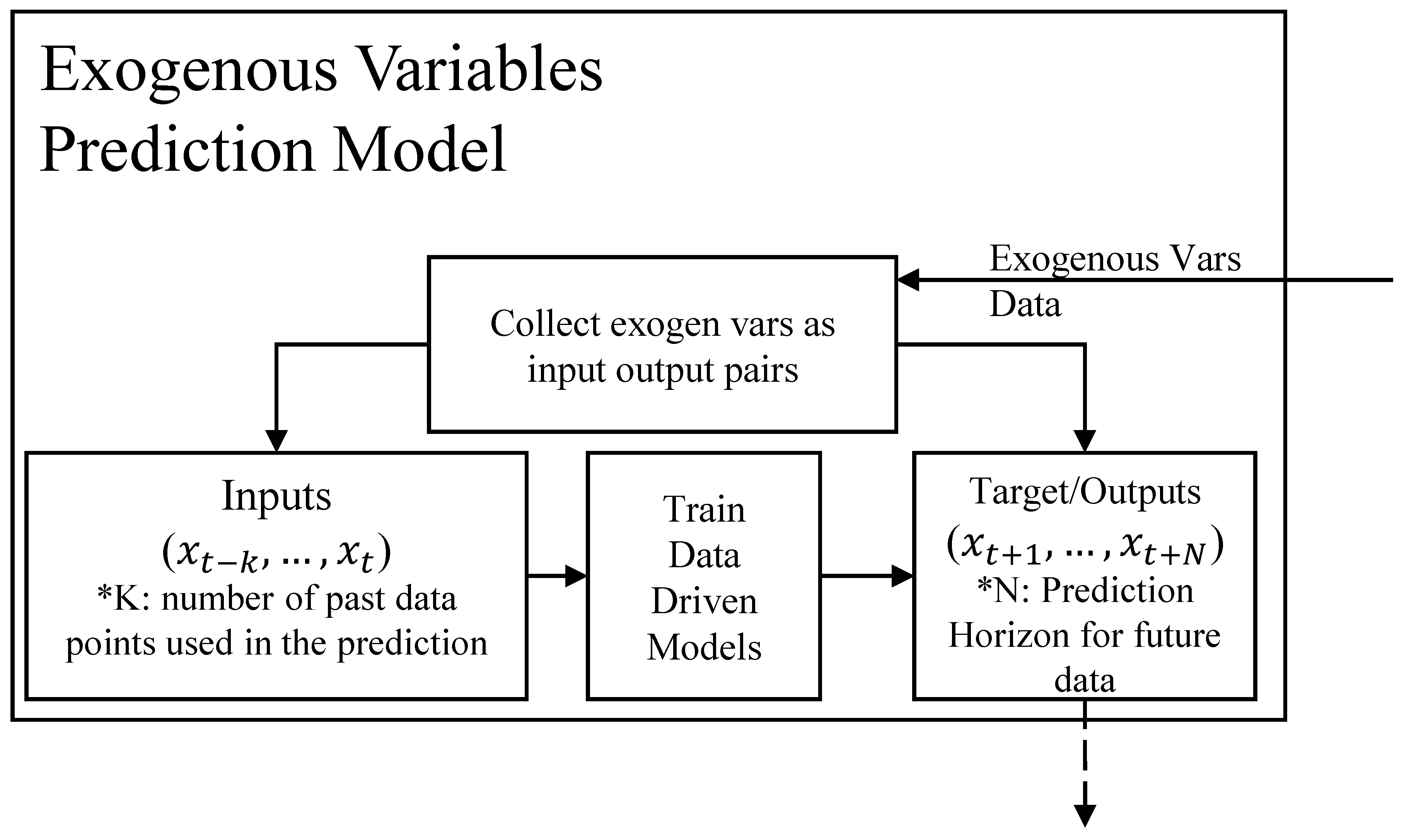
Figure 5.
Schematic of the Five Zone Testbed. Source: [31]
Figure 5.
Schematic of the Five Zone Testbed. Source: [31]
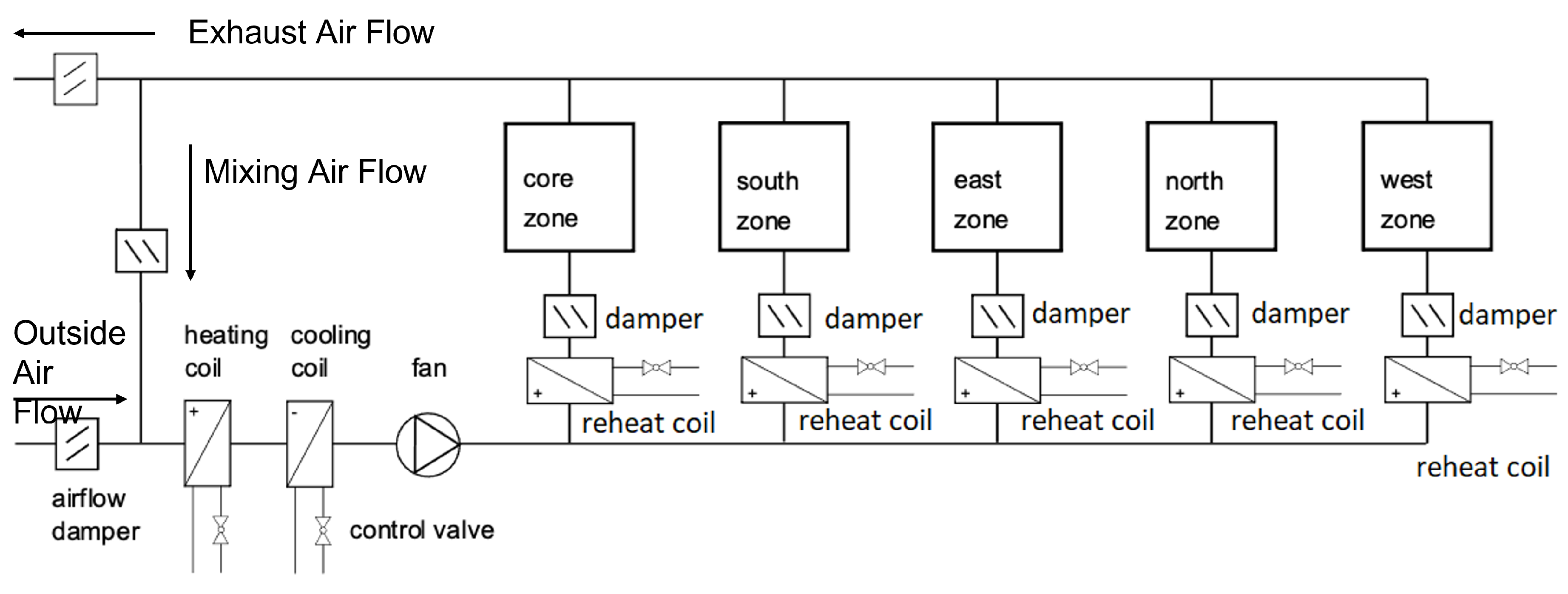
Figure 6.
Bayes Net for the Relearning Approach applied to the 5 Zone Testbed
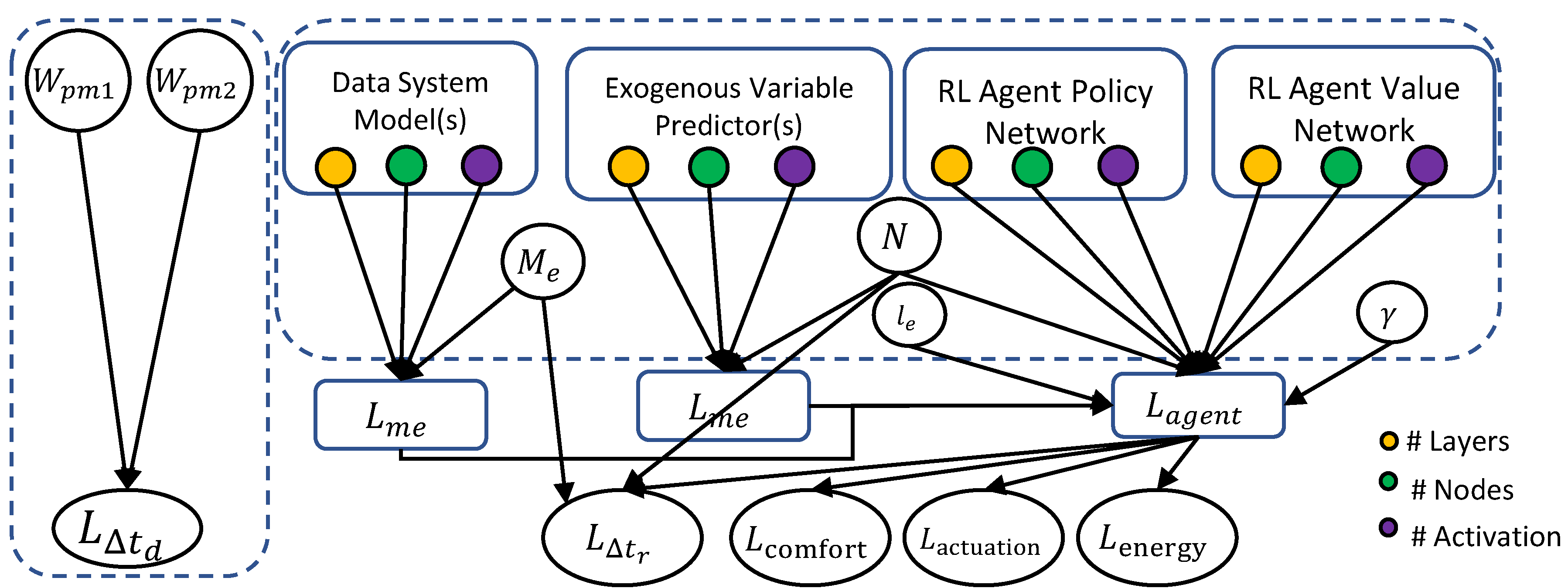
Figure 7.
Performance of Rule-Based, PPO, DDPG, MPPI, and Relearning Approach deployed on the testbed and simulated for a period of 1 year. Benchmarking is done across all types of non-stationarity changes. Metrics are recorded for a week after detection of non-stationarity using the Performance Monitor Module. Energy performance is aggregated for a week. Temperature deviation and Actuation rates are aggregated on a per-hour basis.
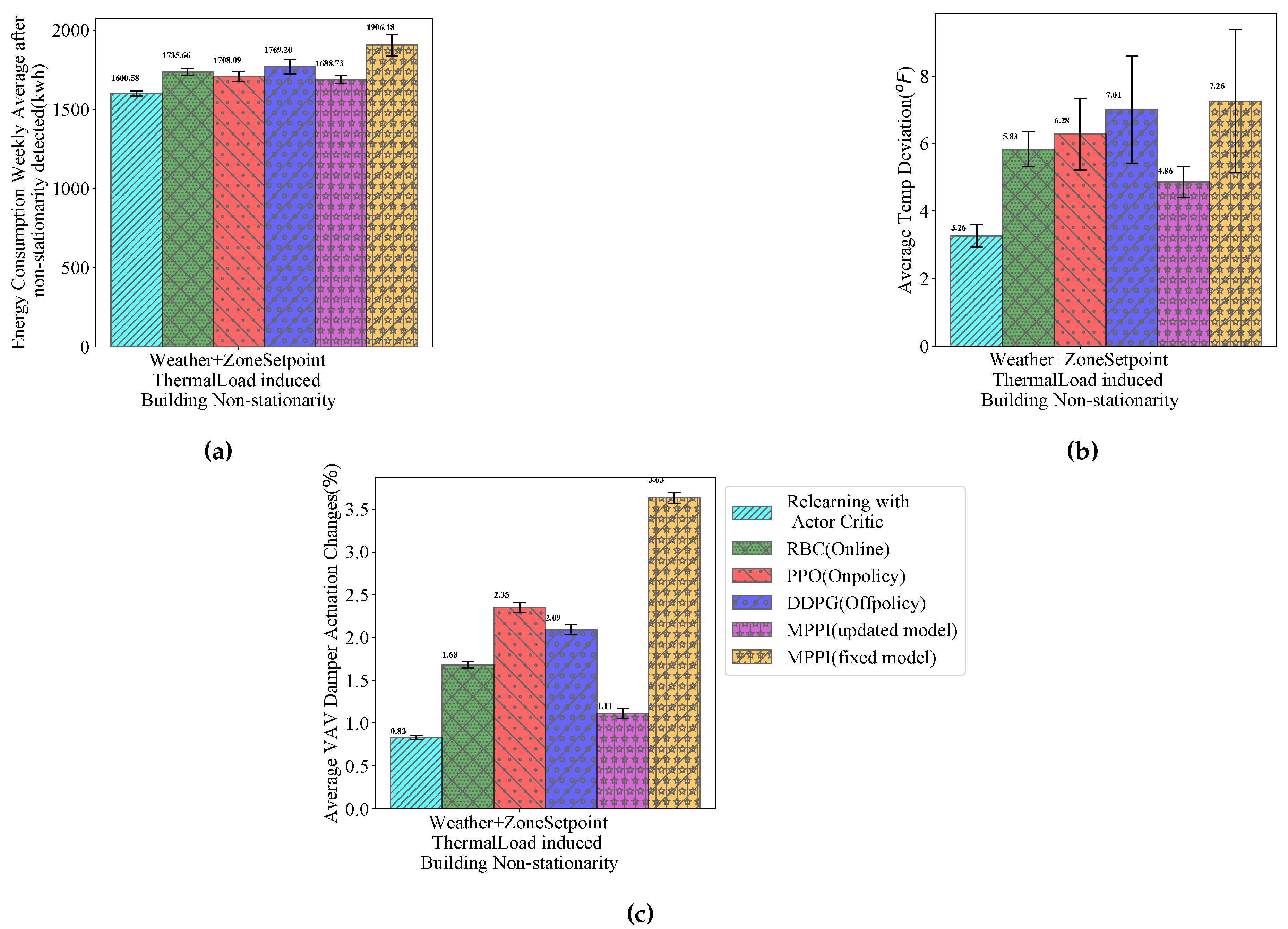
Figure 8.
Total reward obtained for our approach depending on the week and season of the year.
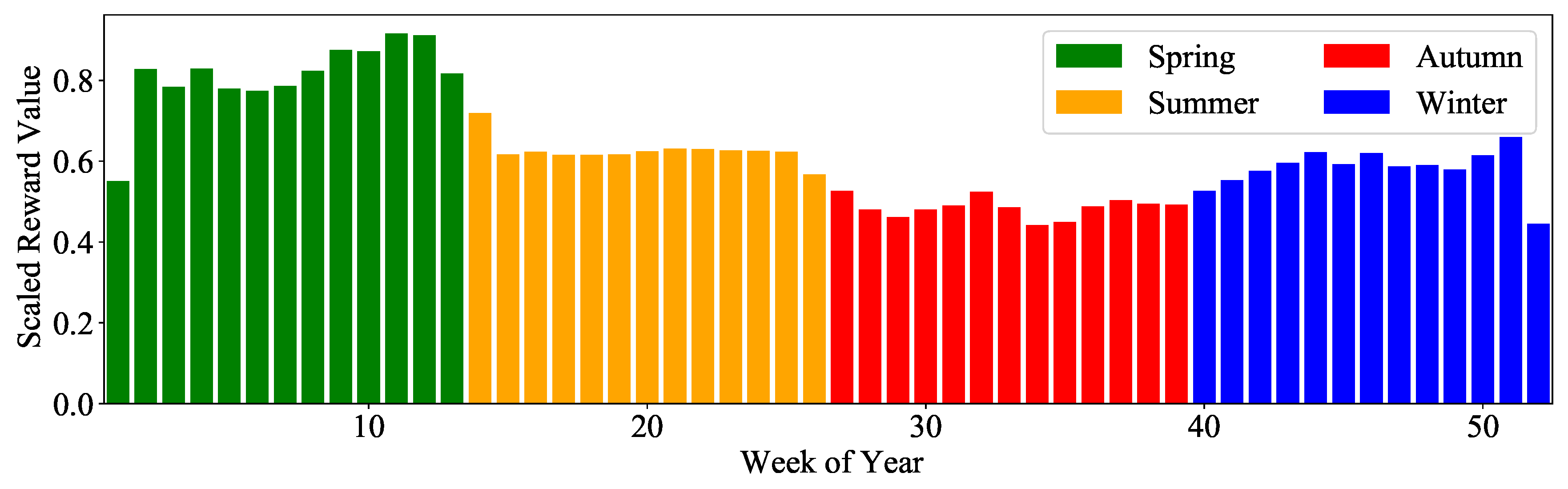
Figure 9.
Total number of relearning phases triggered for our approach depending on the week of the year.
Figure 9.
Total number of relearning phases triggered for our approach depending on the week of the year.
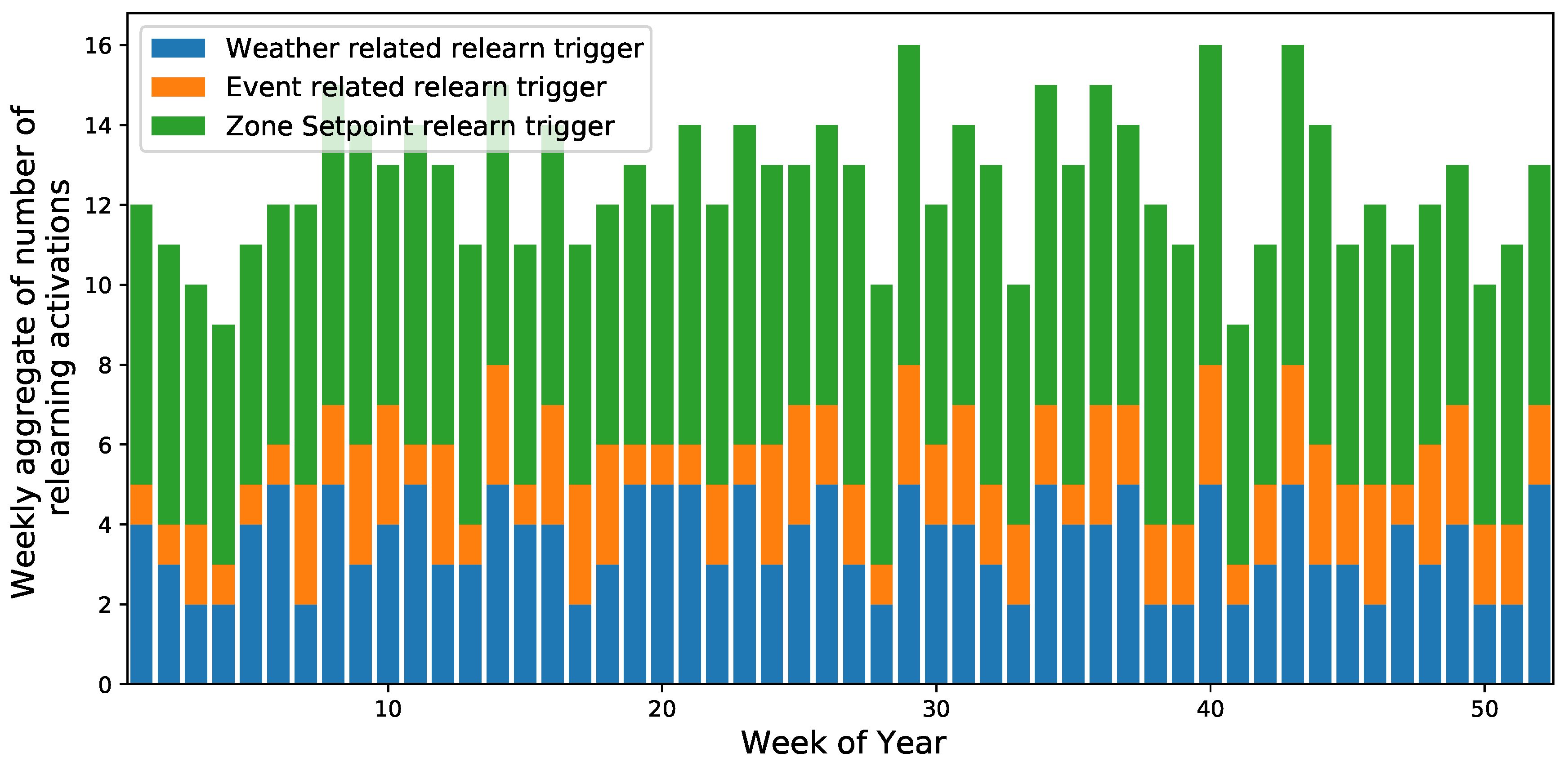

Table 1.
Description of the testbed Dynamic System Model as a non-stationary MDP
| Component | Variables |
|---|---|
| State | 1.Outside Air Temperature(oat) |
| 2.Outside Air Relative Humidity(orh) | |
| 3.Five Zone Temperatures() | |
| 4.Total Energy Consumption() | |
| 5. AHU Discharge Air Temperature () | |
| Action: | AHU Discharge Temperature Set- |
| point () | |
| Reward | where |
| Non-stationary Transition | 1. Total Energy Consumption Model() |
| Model() | 2. Zone Temperature Model() |
| 3. VAV Damper Percentage Model() |
Table 2.
Hyperparameters of the ensemble-CPS pair, the metrics they affect and the classification of the hyperparameters as global or local
Table 2.
Hyperparameters of the ensemble-CPS pair, the metrics they affect and the classification of the hyperparameters as global or local
| Hyperparameter(s) | Metric Affected | Global/Local |
|---|---|---|
| Performance Monitor Module Window sizes: , |
Global | |
| Memory Buffer Size: |
, |
Global |
| Forecast Horizon Length: N |
, . |
Global |
| Exogenous Variable Predictor: Nodes, Layers, Activations |
Local | |
| Dynamic System Model(s): Nodes, Layers, Activations |
Local | |
| RL Agent Policy Network: Nodes, Layers, Activations |
Local | |
| RL Agent Value Network: Nodes, Layers, Activations |
Local | |
| Discount Factor: | Local | |
| Episode Length: | Local |
Table 3.
Ranges of the global hyperparameters
| Hyperparameter | Search Space (Range) |
|---|---|
|
(Performance Monitor Module) |
|
|
(Performance Monitor Module) |
|
| (Experience Buffer) | |
|
N(Exogenous Variable Predictor and Dynamic System Model) |
Table 4.
Ranges of the local hyperparameters
| Hyperparameter | Search Space (Range) |
|---|---|
| Dynamic System Model Weights (, , ) |
|
| Dynamic System Model Activation (, , ) |
|
| Exogenous Variable Model Weights |
|
| Exogenous Variable Model Activation |
|
| Actor() Critic () Network weights |
|
| Actor() Critic () Network Activation |
|
| days |
Table 5.
Tuned values of the input sequence length K and the prediction horizon N under different conditions of non-stationarity.
Table 5.
Tuned values of the input sequence length K and the prediction horizon N under different conditions of non-stationarity.
| Non-stationarity | Weather | Zone Set Point |
Thermal Load |
Combined | ||||
|---|---|---|---|---|---|---|---|---|
| Hyperpara- meter |
K | N | K | N | K | N | K | N |
| Value (hrs) | 18 | 72 | 6 | 72 | 6 | 72 | 12 | 48 |
Table 6.
Tuned values and .
| Non-stationarity | Weather | Zone Setpoint |
||
|---|---|---|---|---|
| Hyperparameter | ||||
| Value (hr) | 6 | 2 | 3 | 2 |
| Non-stationarity | Thermal Load | Combined | ||
| Hyperparameter | ||||
| Value (hr) | 3 | 2 | 6 | 3 |
Disclaimer/Publisher’s Note: The statements, opinions and data contained in all publications are solely those of the individual author(s) and contributor(s) and not of MDPI and/or the editor(s). MDPI and/or the editor(s) disclaim responsibility for any injury to people or property resulting from any ideas, methods, instructions or products referred to in the content. |
© 2025 by the authors. Licensee MDPI, Basel, Switzerland. This article is an open access article distributed under the terms and conditions of the Creative Commons Attribution (CC BY) license (http://creativecommons.org/licenses/by/4.0/).
Copyright: This open access article is published under a Creative Commons CC BY 4.0 license, which permit the free download, distribution, and reuse, provided that the author and preprint are cited in any reuse.


