Submitted:
14 February 2025
Posted:
17 February 2025
You are already at the latest version
Abstract
The rapid development of drone technology has resulted in its ever-expanding applications in the military, commercial, and civilian domains. Nevertheless, the concomitant safety and privacy issues have become increasingly conspicuous, giving rise to an urgent demand for effective monitoring and management of drone activities. Consequently, anti-drone detection and recognition technology has gradually emerged as a research focus. Deep learning provides innovative solutions for drone detection by virtue of its advantages in complex data feature extraction and intelligent signal analysis. In this paper, a UAV audio signal detection method based on GRU neural network and attention mechanism is proposed to solve the limitations of traditional convolutional neural network (CNN) in dealing with background noise and interference signals. In this study, one-dimensional waveform data is converted into a two-dimensional feature space through spectrogram feature extraction of audio signals, so as to capture the global temporal characteristics and dynamic features of UAV audio signals. In the model design, a lightweight two-layer GRU neural network is adopted, which combines the update gate and reset gate mechanisms to effectively capture the short-term and long-term dependencies in the audio signal, avoid the gradient vanishing problem, and improve the computational efficiency and generalization capability. In addition, to further enhance the ability of the model to focus on long time series and complex background signals, an attention mechanism is introduced so that the model can dynamically focus on the information of key time steps, thus improving the robustness of complex signal processing. In order to verify the effectiveness of the proposed method, we conducted experiments on publicly available UAV audio datasets, and the results show that the method proposed in this paper exhibits high detection accuracy and robustness in dealing with the task of UAV audio detection in complex environments, which provides reliable technical support for the development of UAV detection technology.
Keywords:
Drone detection
; security
; privacy
; GRU
; attention
1. Introduction
Due to the rapid development of key technologies in the unmanned aerial vehicle (UAV) industry, such as automatic control, communication technology, and intelligent algorithms, the UAV market is rapidly maturing. And its small size, light weight, good concealment, and strong autonomous flight ability [1], is widely used in tracking, aerial photography, agriculture and forestry operations, military operations, traffic monitoring, rescue and disaster relief, emergency communications, positioning services, aerial mapping, security supply [2] and many other fields.
However, with the booming development of the UAV market, the risk of collision between UAV vehicles and other objects is increasing day by day, which brings a series of safety hazards. At the same time, the deployment of drones may violate some national security policies intentionally or unintentionally [3], and some drones have been used for smuggling, flight disruption, espionage, privacy invasion, and attacks on terror, which have created a series of security threats [4,5] .
In recent years, incidents of “illegal flight” of drones interfering with the operation of airports and flights have been common, which has a serious impact on aviation safety and public travel. In addition, attackers may use drones to carry hazardous materials (e.g., bombs) to carry out attacks, criminals use drones to smuggle illegal materials, and even some operators spy on other people’s privacy through high-definition camera drones [6], etc. In addition, in the military field, some drones have been accused of violating the international conventions on human rights, and thus have been called “malicious drones” [7]. The frequent occurrence of UAV black flight problems highlights the urgency and importance of research on detection and identification techniques for illegal UAV flight behavior.
In order to effectively respond to the security challenges brought about by the development of UAVs, the further development of UAV detection and countermeasure technology has become a key direction of current research. Currently, most relevant research focuses on UAV detection methods based on image, RF signal or radar technologies. However, these methods may face limitations such as occlusion and interference in complex environments, while UAV detection based on acoustic signals is gradually becoming an important research area due to its uniqueness and wide applicability. For example, Andrea Bernardini et al. developed a machine learning-based drone warning system, which extracts multiple short-term features of environmental audio data in the time and frequency domains, and uses Support Vector Machine (SVM) to analyze and identify the audio fingerprints of drones, thus realizing the drone detection and warning functions [8]. In addition, S. Al-Emadi et al. proposed a deep learning based drone detection and recognition method using Convolutional Neural Network (CNN), Recurrent Neural Network (RNN) and Convolutional Recurrent Neural Network (CRN). Convolutional Recurrent Neural Network, RNN, and Convolutional Recurrent Neural Network, CRNN) models, which utilize the unique acoustic fingerprints of drones to achieve detection and identification. This study not only verifies the feasibility of deep learning techniques in UAV detection, but also provides an open-source UAV audio dataset [9], which lays the data foundation for subsequent studies.
Based on this open-source UAV audio dataset, this paper further investigates the performance of various deep learning models in the UAV detection task, including Gated Recurrent Unit (GRU), Long Short-Term Memory (LSTM), and Depth- wise Separable Convolutional Neural Network (DSCN). wise Separable Convolutional Neural Network (DS-CNN). In addition, the performance of these models is compared and analyzed with several common deep learning-based UAV detection methods, including Convolutional Neural Network CNN, Recurrent Neural Network RNN, and Convolutional Recurrent Neural Network CRNN. The experimental results show that the GRU-based UAV detection method performs the best in both detection accuracy and model stability, significantly outperforming the other models, providing an efficient and robust solution for the UAV detection task.
The main contributions of this paper are as folllows:
(1) proposing and validating the effectiveness of combining GRU with the attention mechanism in acoustic signal-based anti-drone detection;
(2) further demonstrating the feasibility and superiority of deep learning techniques in the field of drone audio signal detection through comprehensive performance evaluations, including Accuracy, Loss, Precision, Recall and Recall. Accuracy, Loss, Precision, Recall, and F1 score are included to comprehensively analyze the advantages and disadvantages of different models.
The rest of the paper is structured as follows: section 2 discusses the related work of the study, section 3 describes the dataset used for the experiment and the system model used, section 4 analyzes the experimental results in depth, and section 5 concludes the whole study with an outlook.
2. Related Works
During the flight process of UAV, the operation of motor will generate heat; the rapid rotation of UAV rotor will generate noise; UAV communicates with the remote control end through RF signals, and these processes will generate different characteristic information, which can be collected by different sensors, and then realize the detection and identification of UAV. According to the different types of sensors in the UAV detection system, the existing UAV detection and identification technologies can be divided into the following categories: UAV detection and identification based on image processing, UAV detection and identification based on RF signal processing, UAV detection and identification based on radar technology, UAV detection and identification based on infrared features, and UAV detection and identification based on acoustics.
Drones radiate a large amount of heat from internal hardware such as motors and batteries during flight, and thermal imaging cameras can detect this heat to confirm the presence of a drone [10]. Image processing based drone detection schemes use computer vision and deep learning to detect drones, usually using daylight cameras and infrared or thermal imaging to capture drone images or videos of the monitored area, and based on the object’s appearance characteristics [11], i.e., color, shape, contour, etc., or its motion characteristics across consecutive frames, computer vision based target detection techniques are used to where the UAVs are detected and tracked. Literature [12] proposes a deep learning based approach for effective detection and recognition of drones and birds using YOLO V4 for target detection and recognition, which solves the problem of drone detection under background congestion, area concealment conditions, and the challenge of confusion between drones and birds appearing in visible images. Literature [13] presents a detection dataset of 10,000 images and a tracking dataset of 20 videos covering a wide range of scenarios and target types and uses 14 different detection algorithms to train and evaluate the dataset. Literature [14] proposes a YOLOv5 based UAV detection method that utilizes data augmentation and migration learning techniques to improve detection accuracy and speed.
Drones typically use RF signals from 2.4 GHz to 5 GHz to communicate with controllers, Wi-Fi equipped drones use 5.4 GHz RF signals, 5G drones use 3.5 GHz RF signals, and some of the less common frequency bands are in the range of 1.2 GHz and 1.3 GHz [15]. By extracting spectral features and completing the statistical distribution of RF signals as RF characteristics of the UAV [16], RF sensors can be used to listen to the signals transmitted between the UAV and its controller. Literature [17] proposed a UAV detection and classification method based on convolutional neural network (CNN), which focuses on low-cost and highly robust UAV detection and classification under low signal-to-noise ratio conditions, providing a practical solution for UAV safety monitoring. Literature [18] disclosed a UAV RF signal dataset, which is utilized to record the real data of UAV multi-frequency communication for detecting low altitude UAVs.
Radar transmits radio waves and receives reflected waves from objects. The receiver detects the presence, distance and velocity of the object by analyzing the Doppler shift caused by the moving object [19]. Literature [20] proposed a programmable hypersurface-based UAV detection scheme, which realizes Non Line of Sight (N-LOS) detection of UAVs by designing a full resonance structure and mode alignment technique Literature [21] proposed a CNN-based deep learning technique, which combines the spectral image generated by the radar signals as an input with the visually detected image data for feature extraction to solve the detection problem of small Radar Cross Section (RCS) targets such as UAVs and birds.
At night or in other poorly lit environments, visible light-based UAV detection techniques are no longer applicable due to insufficient light. The infrared detection technique is more resistant to interference, better concealment, and more adaptable, and it is cheaper in terms of price and maintenance, which makes it particularly suitable for dynamic UAV detection performed in low altitude areas. Literature [22] improved the network structure of the SSD algorithm for infrared small target detection, proposed the use of deep learning methods to detect infrared UAV targets, and designed an adaptive pipeline filter based on temporal correlation and motion information to correct the recognition results. However, in practical experiments, the limitation of its resolution makes the accuracy of measurement using infrared thermal camera limited. Meanwhile, during the flight of the UAV, if the temperature of its own radiation and the temperature of the surrounding environment are the same, the ambient temperature also has a certain effect on the infrared measurement.
The rotating blades of UAVs generate unique acoustic signals that can be used to detect and identify UAV models . Propeller blades have relatively high amplitude and are commonly used for detection. The process of capturing acoustic signals using a microphone and processing them, which can be matched with the UAV ID in a database, is known as fingerprinting[23] . Literature [24] proposed an effective Independent Component Analysis (ICA) unsupervised machine learning method for detecting various sounds in real scenarios including birds, airplanes, thunderstorms, rain, wind, and drone sounds.After demixing the signals, ICA is used to extract the Mel- scale Frequency Cepstral Coefficients (MFCC), Power Spectral Density (PSD), and Root Mean Square (RMS) of PSD were extracted using ICA, and the features such as Support Vector Machine (SVM) and K-nearest Neighbor (KNN) were used. Nearest Neighbor (KNN) to classify the detected signals and determine whether there is a UAV signal in the detected signals. Literature [25] proposes a UAV acoustic event detection system based on deep learning and microphone arrays, aiming to achieve high-precision detection of UAV acoustic signals by combining beam forming algorithms and neural networks.
In summary, existing UAV detection methods have their own characteristics. Detection techniques based on image, RF, radar, infrared and acoustic signals play an important role in different application scenarios, but they also face problems such as environmental interference, target occlusion, complex backgrounds and harsh climate, which impose different degrees of limitations on detection performance. UAV detection technology based on acoustic signals has gradually become a research hotspot due to its advantages of low cost, high adaptability, and strong anti-interference ability. Acoustic detection does not need to rely on light conditions, performs particularly well in low light and complex weather, and is able to effectively recognize UAVs through the unique acoustic characteristics of rotor blades. However, acoustic detection methods also face the challenges of environmental noise interference and limited detection range, so they need to be combined with deep learning models to mine the key features in the audio signal, so as to improve the detection accuracy and robustness. In this paper, we address this research direction and thoroughly study the performance of various deep learning models in UAV detection tasks, including gated recurrent unit (GRU), long-short-term memory network (LSTM), and deep separable neural network (DS-CNN), and propose a UAV audio signal detection method based on GRU neural network and attention mechanism, aiming to fully exploit the time-series features and the frequency-contrast mechanisms in the audio signal of UAVs. time series features and spectral information in the signals, providing multi-dimensional feature expression capability for UAV detection tasks.
3. Dataset and System Model
An experimental dataset dedicated to UAV audio signal detection is used in this study. A review of the relevant literature reveals that this dataset was proposed by the authors and proved to be suitable for this study. The dataset contains more than 1300 segments of UAV audio data to simulate complex scenarios in real life. To enhance the versatility and adaptability of the dataset, the authors also introduced noise segments from publicly available noise datasets to examine the robustness and detection ability of the model in a noisy environment.
Materials and Methods should be describeAn experimental dataset dedicated to UAV audio signal detection is used in this study. A review of the relevant literature reveals that this dataset was proposed by the authors and proved to be suitable for this study. The dataset contains more than 1300 segments of UAV audio data to simulate complex scenarios in real life. To enhance the versatility and adaptability of the dataset, the authors also introduced noise segments from publicly available noise datasets to examine the robustness and detection ability of the model in a noisy environment.
The dataset covers the audio signals of two different UAV models, namely Bebop and Mambo.The audio recording of each UAV has a duration of 11 minutes and 6 seconds, with a sampling rate of 16 kHz, mono, and a maximum audio bit rate of 64 kbps.All the audio files are stored in the MPEG-4 audio format, which ensures efficient storage and transmission of the data.
In order to meet the requirements of feature learning in deep learning models, the audio files are divided into multiple smaller segments, and the optimal solution is the 1-second segmentation, which is determined through experiments. After this processing, the audio data not only retains the complete timing characteristics, but also facilitates efficient training and learning of the model with limited computational resources.
This study can be roughly divided into three steps: audio feature extraction, feature processing and modeling, and classification prediction. Firstly, spectrogram feature extraction is performed on the audio data in the dataset, which converts the one-dimensional waveform data into a two-dimensional spectrogram feature space; then the extracted spectrogram features are reshaped and global features in the time series are extracted by a two-layer gated recurrent unit (GRU) network, and at the same time, high-dimensional features are combined with the fully-connected layer to perform the dimensionality reduction process, and then regularization is performed by the Dropout layer to reduce the over regularization through Dropout layer to reduce the risk of overfitting. Finally, the Softmax output layer is used to generate the UAV audio detection and classification results to realize the classification prediction of UAV audio. The overall structure flow chart is shown in Figure 1:
Features extracted from audio signals mainly include time domain features and frequency domain features. Time-domain features are the simplest and most direct features extracted from the sampled signal with time as the independent variable. However, generally through the time domain analysis can only get the power change of the acoustic signal, can not judge the frequency components contained in the acoustic signal, so it should be analyzed from the frequency domain features. The time-domain signal of the acoustic signal can be converted to the frequency domain by Fourier transform to obtain the corresponding phase spectrum and amplitude spectrum, from which the amplitude spectrum can be used to analyze the frequency components of the signal and obtain the energy distribution of different frequency components during the time. As a result, the frequency domain features of the sound signal can be extracted. The frequency domain features include Meier frequency cepstrum coefficient features, logarithmic amplitude spectral features, logarithmic Meier filter bank energy features, perceptual linear prediction features, Gammatone frequency cepstrum coefficient features, and power regularization cepstrum coefficient features.
Linear predictive cepstral coefficient (LPCC) and Mel frequency cepstral coefficient (MFCC) as two common sound signal feature extraction techniques.MFCC is a method of speech analysis based on the human hearing mechanism, which analyzes the spectrum of speech by simulating the perceptual characteristics of the human ear to the sound signal. The computational process of MFCC mainly includes the following steps: firstly, the time domain signal is segmented and converted to the frequency domain by Short-Time Fourier Transform (STFT). Subsequently, the frequency components on the Meier frequency scale are extracted by a set of triangular filters using the Meier filter bank. And then the filtered energy is logarithmically taken to enhance the small signal variations. Finally, the logarithmic energy spectrum is converted into cepstrum coefficients using the Discrete Cosine Transform (DCT), which reduces the redundant information and retains the main energy.LPCC is a cepstrum feature extraction method based on linear predictive analysis, which analyzes the spectral structure of audio signals by predicting the relationship between the current signal values and the past signal values. However, LPCC tends to retain some redundant information that is not related to the signal, which leads to the degradation of classification performance, so MFCC is chosen as the main feature extraction method in this study. The acoustic spectrograms of some drones and noises as well as the cepstrum of Mel’s frequency spectrum are shown in Figure 2, respectively:
Assuming that the input UAV audio signal is , the frame length is L , the frame shift is , and the audio signal is subjected to sub-framing to divide the time-domain signal into multiple sub-frames, the signal in the first frame is:
To minimize spectral leakage, the signal is windowed. For each frame of the signal , the window function is applied:
The Hamming window used in this study is:
Project the time domain signal into the time-frequency domain by Short Time Fourier Transform (STFT) to obtain the frequency domain representation of the signal, including the magnitude and phase spectra:
where is the frequency domain representation of the k-th frame signal, w denotes the frequency variable, and denotes the signal after adding a window to the k-th signal., the output of the STFT contains the magnitude and phase spectra.
The magnitude spectrum provides the energy distribution of the signal:
The phase spectrum provides the phase information of the signal:
The Mel filter set is used to simulate the auditory properties of the human ear, emphasizing the sensitive frequency range of the human ear (e.g., 300 4000 Hz) and converting the frequency axis to the Mel Scale. A set of Mel filters is used to filter the amplitude spectrum and extract the energy information on the Mel Frequency Scale, and the relationship between the frequency (Hz) and the Mel Frequency is as follows:
Assuming that the magnitude spectrum passing through the STFT is , the Mel filter bank is weighted and summed by a set of triangular filters as follows:
where denotes the output energy of the m-th Mel filter, M denotes the weight of the m-th Mel filter, and is the number of Mel filters. Each filter’s is triangular in shape and has a peak at the center frequency corresponding to the Meier frequency.
Taking logarithms of the output of each Meier filter enhances the variation of low-energy signals:
where denotes a very small positive number to avoid the logarithm going to infinity.
The Discrete Cosine Transform (DCT) converts the logarithmic energy into cepstrum coefficients and removes the redundant information from the features to obtain the Mel frequency cepstrum coefficients (MFCC):
where denotes the n-th Mel frequency cepstrum coefficient, M denotes the number of Mel filter banks, and N denotes the number of retained Mel frequency cepstrum coefficients.
The original input signal is a two-dimensional signal obtained by STFT, which needs to be feature reshaped to include time dimension as well as frequency dimension information, and the two-dimensional features of the spectrogram are adjusted to the three-dimensional time series data required by the GRU network (the batch size, the time step, and the feature size of each time step), and the spectrogram features are reshaped to fit the input requirements of the GRU network Input Features:
Reshape after reshaping:
In the global feature extraction part, the time series information of audio features is extracted using a two-layer GRU network to capture the long-term dependencies in the audio signal. The first layer GRU retains the features at each time step and extracts the coarse-grained features of the sequence and passes them to the second layer GRU, which does not retain the time step sequence and outputs the final high-level features for higher-level feature extraction. The GRU network contains two gates inside, the update gate as well as the reset gate. The GRU model is shown in Figure 3:
Update Gate determines how much of the current timestep’s state will be updated:
Reset gate controls the effect of the previous hidden state on the current computation:
Candidate hidden state is the candidate value for the current hidden state:
Hidden state represents a weighted update using the update gate directly between the previous hidden state and the new candidate hidden state:
where, denotes the input of the current time step, denotes the hidden state of the current time step, denotes the hidden state of the previous time step, and represent the update gate and reset gate, respectively. W, U, and b represent the input-to-hidden state weight matrix, the hidden state-to-hidden state weight matrix, and the bias, respectively, and denotes the sigmoid activation function, tanh denotes the tanh activation function, and ⊙ denotes the element-by-element multiplication.
For the input hidden state sequence from the GRU, the ATTENTION mechanism first calculates the attention score for each time step, which is used to indicate the degree of contribution of each time step in the input sequence to the output:
where and are the learnable weight matrix and bias.
The attention scores are converted to weight distributions by the softmax activation function:
where denotes the attentional weights of the time step that satisfies , T representing the total time step.
The context vector c is the weighted sum of the input hidden states, which is used to represent the global information attended by the model:
where denotes the attentional weight, and denotes the input hidden state. The context vector is incorporated into the GRU hidden state update formula for further feature extraction and classification of the subsequent network as follows:
Update gate :
Reset gate :
Candidate hidden state :
Final hidden state :
Where, denotes the input of the current time step, denotes the hidden state of the previous time step, denotes the weight matrix from the input to the corresponding gate, denotes the weight matrix from the previous hidden state to the corresponding gate, and denotes the bias term of the corresponding gate. The overall architecture is shown in Figure 4.
The high-dimensional features are downscaled and mapped to the low-dimensional space using a Dense (fully connected) layer with the mathematical expression:
where W denotes the weight matrix, h denotes the hidden state, b denotes the bias, and denotes the activation function used in this study (typically, could represent a function like sigmoid, ReLU, etc.).
The Dropout layer randomly discards some neurons to avoid overfitting the model to the training data:
where p is the retention probability, m is the randomly generated binary matrix used to discard neurons, h is the original features, and is the features after dropout processing.
After GRU and fully connected layer processing of the features, the Softmax layer is used to generate the output probability distribution, indicating the probability that the audio data belongs to each category, and the final classification result is determined according to the maximum value of the output probability:
Where, denotes the output score of the k-th category, K denotes the total number of categories, and denotes the probability that the input belongs to the k-th category.
The accuracy rate is used to indicate the proportion of correctly predicted samples to the total samples by the model:
where, denotes that the true label is positive and the prediction is also positive; denotes that the true label is negative and the prediction error is positive; denotes that the true label is negative and the prediction is negative; denotes that the true label is positive and the prediction error is negative.
The sparse classification cross-entropy loss function is suitable for multi-classification tasks where the labels are integer coded:
where, N denotes the number of samples, denotes the true label of the i-th sample, and denotes the probability of the true category in the i-th sample predicted by the model.
The precision is used to measure how many of the samples that are positive in the model prediction are true positive samples:
Recall is used to measure how many of all true samples are correctly predicted as positive:
The F1-score is a reconciled average of Precision and Recall, which combines measures of model precision and recall:
When precision and recall are close, the F1-score is also higher; if precision or recall is very low, the F1-score is also significantly lower. In summary, our proposed method for UAV audio signal detection based on GRU with attention mechanism, i.e., GRU-ANET can be summarized as Algorithm 1.
| Algorithm 1: GRU-Based Drone Audio Detection Framework |
|
4. Results
To validate the feasibility and effectiveness of our proposed GRU-ANET algorithm, we conducted experiments on publicly available UAV audio datasets. The purpose of the experiments is to evaluate the performance of the proposed method in the UAV detection task and compare it with existing mainstream methods (CNN, DNN, CRNN, DS-CNN, LSTM). The detailed description of the experiments and the analysis of the results are given below.
In order to prevent overfitting, i.e., as the training Epoch increases, the loss of the model continues to decrease on the training set, but on the validation set, the loss may stop improving or even start to rise at a certain point, we introduce the EarlyStopping early-stopping mechanism in our experiments. We introduce the EarlyStopping mechanism in our experiments, which terminates the training when the loss in the validation set stops improving within a certain number of Epochs, thus preventing the model from overfitting the training data and saving the training time effectively. As a result, the number of training Epochs varies from model to model. The accuracy of different models on the training and validation sets and the variation of the loss with the training epoch are shown in Figure 5 and 6, respectively.
From Figure 5, we can see that GRU-ANET, DS-CNN and DNN models perform the best, with a training accuracy close to 99% and a stable training process, while LSTM and CRNN models perform the second best, but also achieve a high training accuracy (about 97%-98%).GRU-ANET and DS-CNN perform the best on the validation set, with a final accuracy of over 98% and a high generalization ability. above 98% with strong generalization ability.
As can be seen from Figure 6, the training loss of all models decreases gradually with the increase of Epoch, especially in the first 3 Epochs, indicating that the models are able to fit the training data quickly.The DS-CNN, GRU-ANet and DNN models have the lowest training loss, which indicates that these models can converge quickly. In the validation loss part, DS-CNN and GRU-ANet models have the lowest and stable validation loss, indicating that they have good generalization ability. Overall, our proposed UAV audio signal detection method based on GRU neural network with attention mechanism performs well.
To further verify the reliability of the experimental results, we introduce three evaluation metrics: Precision, Recall and F1 score, which can more comprehensively evaluate the performance of the model in detecting UAV audio signals. We also drew a comparison graph of the detection effect of different models on UAVs, as shown in Figure 7.
Figure 7 shows the performance of CNN, DNN, DS-CNN, LSTM, CRNN, and GRU models in the UAV audio detection task in terms of Precision, Recall, and F1-score.The GRU model once again performs the best with Precision: 99.89%, Recall: 99.38%, and F1-score: 99.63%, all of which are the highest. The GRU model performs well in UAV audio detection, with the highest recall rate, which can effectively reduce missed detections and has the best overall performance.
In addition, we also draw the Precision-Recall curve (shown in Figure 8) to evaluate the performance of the GRU + Attention mechanism-based method in the task of UAV audio signal detection, and it can be found that the Precision-Recall curve still maintains a higher Precision in a higher Recall range, which indicates that the method can effectively reduce the leakage of audio when detecting UAVs. It can be found that the Precision-Recall curve still maintains a high Precision in a high Recall range, indicating that the method can effectively reduce the leakage detection while maintaining a low false detection rate in detecting UAV audio.
In order to verify the actual role of the attention mechanism in the model, we conducted an ablation experiment at the end of the experiment, trained the models with and without the attention mechanism respectively, and analyzed their performance, and the results are shown in Figure 9. It can be found that the model with the attention mechanism (red solid line) converges faster in the early stage of training, its validation loss is lower in all Epochs compared to the model without the attention mechanism (blue dashed line), and the accuracy of the model with the attention mechanism (red dashed line) is better than that of the model without the attention mechanism (blue solid line) in both the training and validation sets.
Comparing the response time of different models in the task, including the training time and the time required for validation, as shown in Table 1, it can be found that:DS-CNN and our proposed model GRU-ANET achieve higher performance with the lowest training time and the shortest inference time.
In summary, we believe that the GRU-ANet model performs excellently in terms of detection accuracy, robustness and response time, and is ideal for coping with UAV detection tasks. Meanwhile, the detection performance of the model in complex environments is further improved by introducing the attention mechanism.The GRU-ANet model not only achieves high accuracy in both noise detection and audio classification tasks in UAV audio signal detection (99.37% and 95.49% F1 scores, respectively), but also performs stably on the validation set with strong generalization ability. Compared with other mainstream models (e.g., CNN, DNN, LSTM, CRNN, etc.), the GRU-ANet model demonstrates higher detection accuracy and lower false and missed detection rates, which further validates its superiority in the field of UAV detection. In addition, the practical role of the attentional mechanism was further verified by ablation experiments. The results show that the GRU model with the attention mechanism not only converges faster in the training phase compared to the model without the attention mechanism, but also the validation loss and accuracy are both GRU-ANet significantly improved. It shows that the attention mechanism has an important role in the feature extraction part.
5. Conclusion
In this study, a UAV audio signal detection method based on GRU neural network with attention mechanism is proposed, aiming to solve the shortcomings of traditional methods in complex environments. Through systematic experimental validation on publicly available UAV audio datasets, the advantages of the GRU network in temporal feature processing are fully utilized and combined with the attention mechanism to dynamically focus on the key time steps, which significantly enhances the model’s ability to recognize UAV audio signals. Experimental results show that the method in this paper performs well in the detection task on the publicly available UAV audio dataset, and outperforms the traditional method in evaluation metrics such as accuracy, recall, and F1 score. Overall, the UAV audio signal detection method proposed in this paper not only improves the detection accuracy, but also significantly reduces the complexity of the model, which provides a new idea for technological innovation in the field of UAV detection.
In order to further improve the robustness and practicality of the model, future research can combine multimodal signals, such as fusing audio signals with other sensor data, such as visual, radar, or infrared signals, in order to cope with UAV detection tasks in more complex environments. Multimodal signals can provide more multi-dimensional information, enabling the model to effectively respond to different disturbances and environmental changes, thus improving its adaptability and reliability. In addition, future work can further explore the potential of fusing mixed signals with multimodal data, especially in complex environments, and investigate its adaptability enhancement in noisy environments, occlusions, and diverse scenarios.
Author Contributions
Conceptualization: Zhongqiang Luo; Methodology: Lan Xu; Investigation:Xiang Dai; Writing–original draft preparation: Lan Xu; Writing–review and editing: Zhongqiang Luo; Supervision: Zhongqiang Luo; Project administration: Zhongqiang Luo; Funding acquisition: Zhongqiang Luo. All authors have read and agreed to the published version of the manuscript
Funding
This work was supported in part by the National Natural Science Foundation of China under Grant 61801319, in part by the Sichuan Science and Technology Program under Grant 2020JDJQ0061 and 2021YFG0099, in part by the Opening Project of Artificial Intelligence Key Laboratory of Sichuan Province under Grant 2021RZJ01, in part by the Scientific Research and Innovation Team Program of Sichuan University of Science and Engineering under Grant SUSE652A011, in part by the Postgraduate Innovation Fund Project of Sichuan University of Science and Engineering under Grant Y2024299.
Institutional Review Board Statement
Not applicable.
Informed Consent Statement
Not applicable.
Data Availability Statement
The data presented in this study are available from the corresponding author upon request.
Conflicts of Interest
The authors declare no conflict of interest.
References
- Anwar, M.Z.; Kaleem, Z.; Jamalipour, A. Machine learning inspired sound-based amateur drone detection for public safety applications. IEEE Transactions on Vehicular Technology 2019, 68, 2526–2534. [Google Scholar] [CrossRef]
- Kaleem, Z.; Yousaf, M.; Qamar, A.; Ahmad, A.; Duong, T.Q.; Choi, W.; Jamalipour, A. UAV-empowered disaster-resilient edge architecture for delay-sensitive communication. IEEE Network 2019, 33, 124–132. [Google Scholar] [CrossRef]
- Kaleem, Z.; Chang, K. Public safety priority-based user association for load balancing and interference reduction in PS-LTE systems. IEEE access 2016, 4, 9775–9785. [Google Scholar] [CrossRef]
- Harkins, G. Illicit drone flights surge along us-mexico border as smugglers hunt for soft spots. shorturl. at/moqG1, 2020. [Google Scholar]
- Schmidt, M.S.; Shear, M.D. A drone, too small for radar to detect, rattles the white house. The New York Times 2015, 26. [Google Scholar]
- Shi, X.; Yang, C.; Xie, W.; Liang, C.; Shi, Z.; Chen, J. Anti-drone system with multiple surveillance technologies: Architecture, implementation, and challenges. IEEE Communications Magazine 2018, 56, 68–74. [Google Scholar] [CrossRef]
- Yaacoub, J.P.; Noura, H.; Salman, O.; Chehab, A. Security analysis of drones systems: Attacks, limitations, and recommendations. Internet of Things 2020, 11, 100218. [Google Scholar] [CrossRef] [PubMed]
- Bernardini, A.; Mangiatordi, F.; Pallotti, E.; Capodiferro, L. Drone detection by acoustic signature identification. electronic imaging 2017, 29, 60–64. [Google Scholar] [CrossRef]
- Al-Emadi, S.; Al-Ali, A.; Mohammad, A.; Al-Ali, A. Audio based drone detection and identification using deep learning. In Proceedings of the 2019 15th International Wireless Communications &, 2019, Mobile Computing Conference (IWCMC). IEEE; pp. 459–464.
- Guvenc, I.; Koohifar, F.; Singh, S.; Sichitiu, M.L.; Matolak, D. Detection, tracking, and interdiction for amateur drones. IEEE Communications Magazine 2018, 56, 75–81. [Google Scholar] [CrossRef]
- Zhang, Z.; Cao, Y.; Ding, M.; Zhuang, L.; Yao, W. An intruder detection algorithm for vision based sense and avoid system. In Proceedings of the 2016 International Conference on Unmanned Aircraft Systems (ICUAS). IEEE; 2016; pp. 550–556. [Google Scholar]
- Samadzadegan, F.; Dadrass Javan, F.; Ashtari Mahini, F.; Gholamshahi, M. Detection and recognition of drones based on a deep convolutional neural network using visible imagery. Aerospace 2022, 9, 31. [Google Scholar] [CrossRef]
- Bo, C.; Wei, Y.; Wang, X.; Shi, Z.; Xiao, Y. Vision-based anti-UAV detection based on YOLOv7-GS in complex backgrounds. Drones 2024, 8, 331. [Google Scholar] [CrossRef]
- Seidaliyeva, U.; Akhmetov, D.; Ilipbayeva, L.; Matson, E.T. Real-time and accurate drone detection in a video with a static background. Sensors 2020, 20, 3856. [Google Scholar] [CrossRef] [PubMed]
- Nguyen, P.; Ravindranatha, M.; Nguyen, A.; Han, R.; Vu, T. Investigating cost-effective RF-based detection of drones. In Proceedings of the Proceedings of the 2nd workshop on micro aerial vehicle networks, systems, and applications for civilian use, 2016, pp.
- Ryden, H.; Redhwan, S.B.; Lin, X. Rogue drone detection: A machine learning approach. In Proceedings of the 2019 IEEE Wireless Communications and Networking Conference (WCNC). IEEE; 2019; pp. 1–6. [Google Scholar]
- Glüge, S.; Nyfeler, M.; Aghaebrahimian, A.; Ramagnano, N.; Schüpbach, C. Robust Low-Cost Drone Detection and Classification Using Convolutional Neural Networks in Low SNR Environments. IEEE Journal of Radio Frequency Identification 2024. [Google Scholar] [CrossRef]
- Yu, N.; MAO, S.; ZHOU, C.; SUN, G.; SHI, Z.; CHEN, J. DroneRFa: a large-scale dataset of drone radio frequency signals for detecting low-altitude drones. J. Electron. Inf. Technol 2023, 45, 1–10. [Google Scholar]
- Doviak, R.J.; Zrnic, D.S.; Sirmans, D.S. Doppler weather radar. Proceedings of the IEEE 1979, 67, 1522–1553. [Google Scholar] [CrossRef]
- Chu, H.; Zhao, H.; Li, P.; Guo, Y.X. Urban skies safeguarded: innovative drone detection with programmable metasurface periscope. Nature Communications 2024, 15, 10375. [Google Scholar] [CrossRef] [PubMed]
- Abdelsamad, S.E.; Abdelteef, M.A.; Elsheikh, O.Y.; Ali, Y.A.; Elsonni, T.; Abdelhaq, M.; Alsaqour, R.; Saeed, R.A. Vision-Based Support for the Detection and Recognition of Drones with Small Radar Cross Sections. Electronics 2023, 12, 2235. [Google Scholar] [CrossRef]
- Ding, L.; Xu, X.; Cao, Y.; Zhai, G.; Yang, F.; Qian, L. Detection and tracking of infrared small target by jointly using SSD and pipeline filter. Digital signal processing 2021, 110, 102949. [Google Scholar] [CrossRef]
- Schauer, L.; Dorfmeister, F.; Wirth, F. Analyzing passive Wi-Fi fingerprinting for privacy-preserving indoor-positioning. In Proceedings of the 2016 International Conference on Localization and GNSS (ICL-GNSS). Ieee; 2016; pp. 1–6. [Google Scholar]
- Uddin, Z.; Altaf, M.; Bilal, M.; Nkenyereye, L.; Bashir, A.K. Amateur Drones Detection: A machine learning approach utilizing the acoustic signals in the presence of strong interference. Computer Communications 2020, 154, 236–245. [Google Scholar] [CrossRef]
- Sun, Y.; Li, J.; Wang, L.; Xv, J.; Liu, Y. Deep Learning-based drone acoustic event detection system for microphone arrays. Multimedia Tools and Applications 2024, 83, 47865–47887. [Google Scholar] [CrossRef]
Figure 1.
Overall structure flow chart
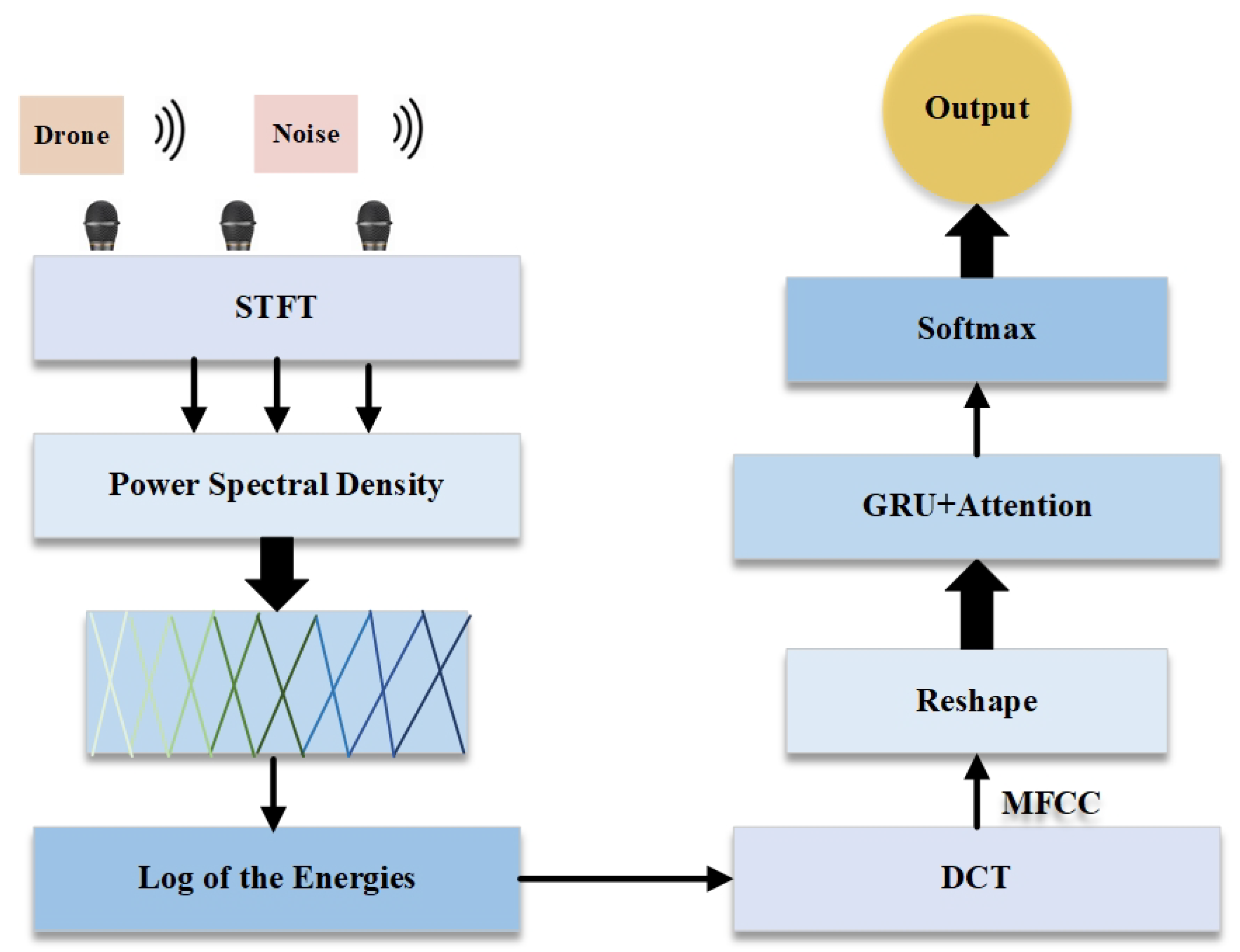
Figure 2.
Acoustic spectrograms of some drones and noises and the cepstrum of the Meier spectrum
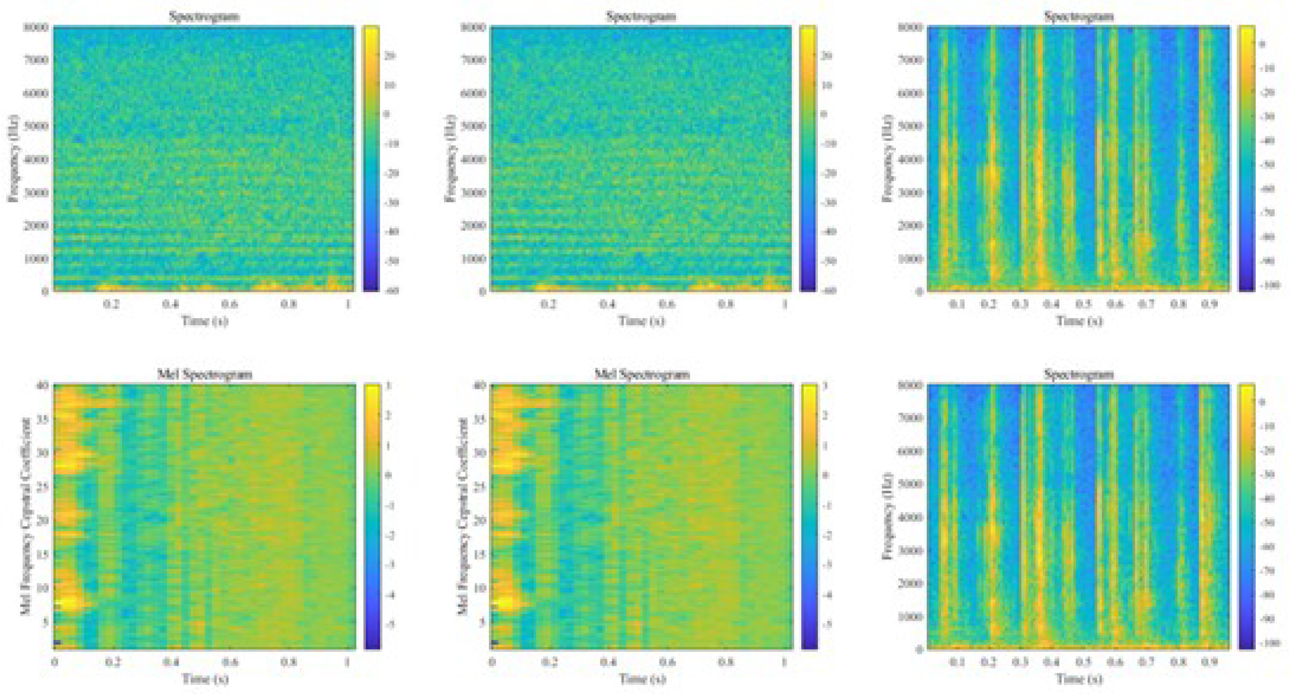
Figure 3.
GRU network architecture
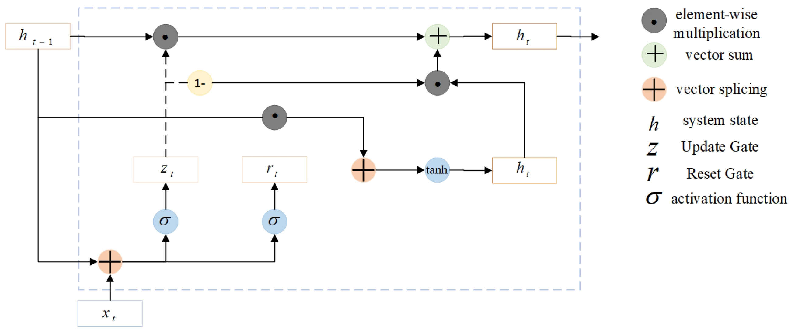
Figure 4.
GRU-ANet architecture diagram
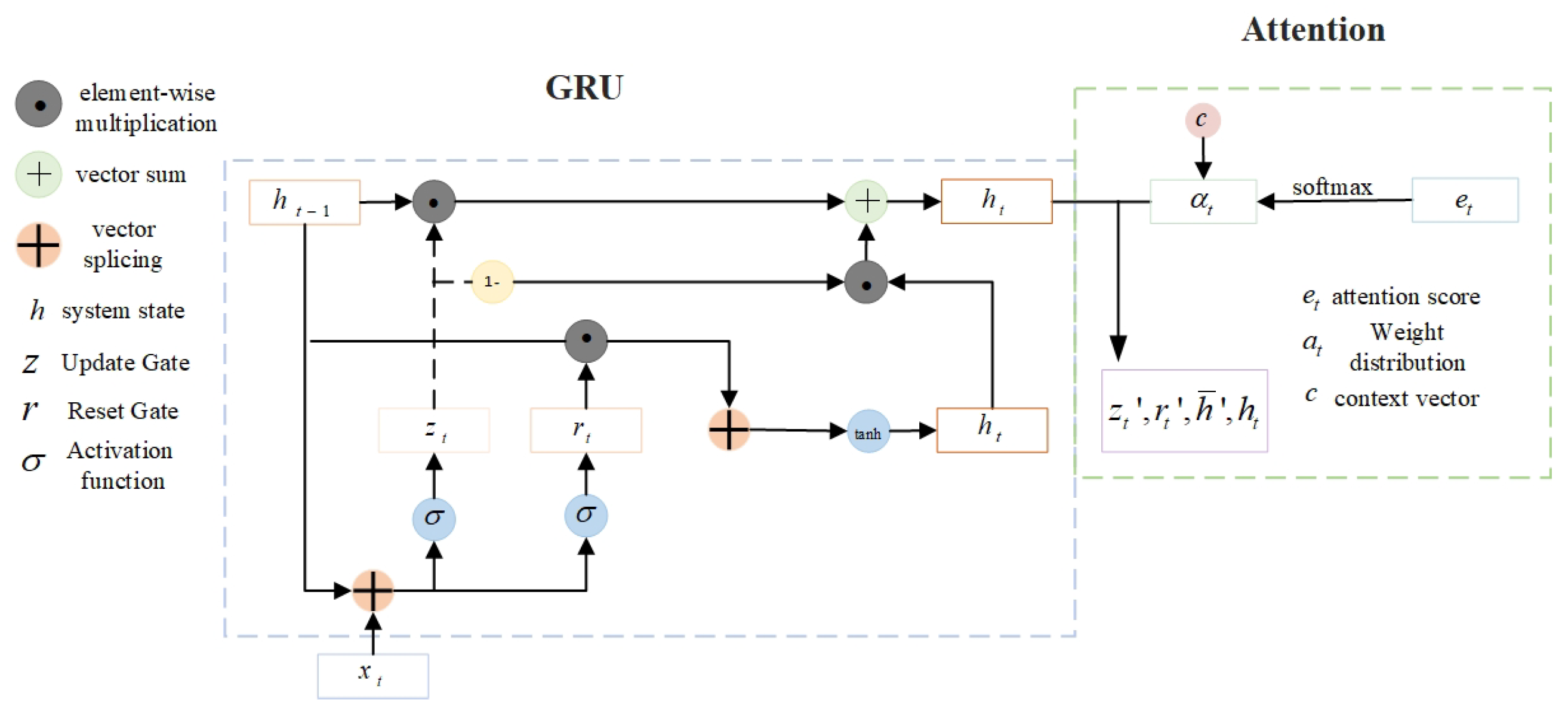
Figure 5.
Comparison of training and validation accuracy.
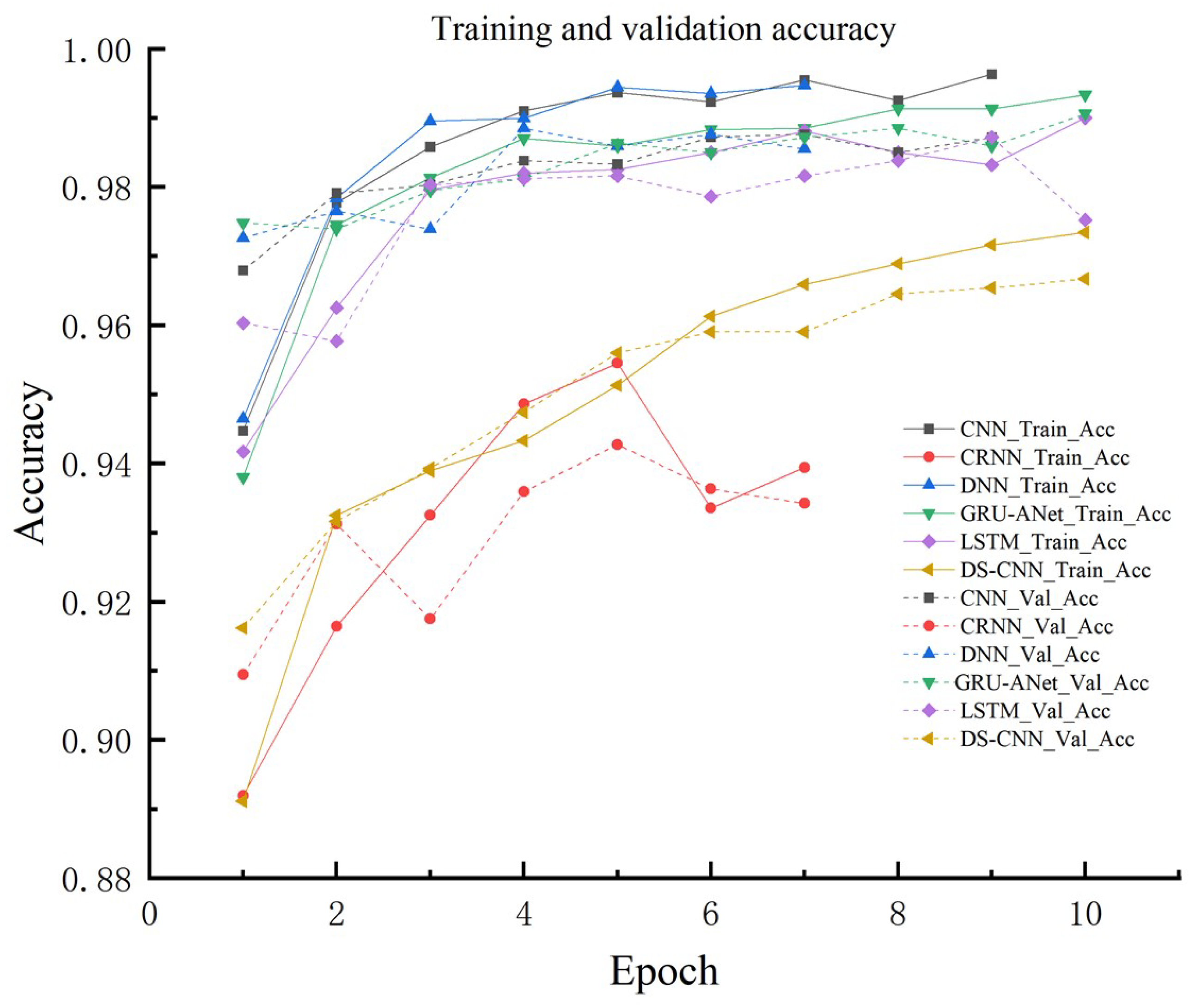
Figure 6.
Comparison of training and validation loss.
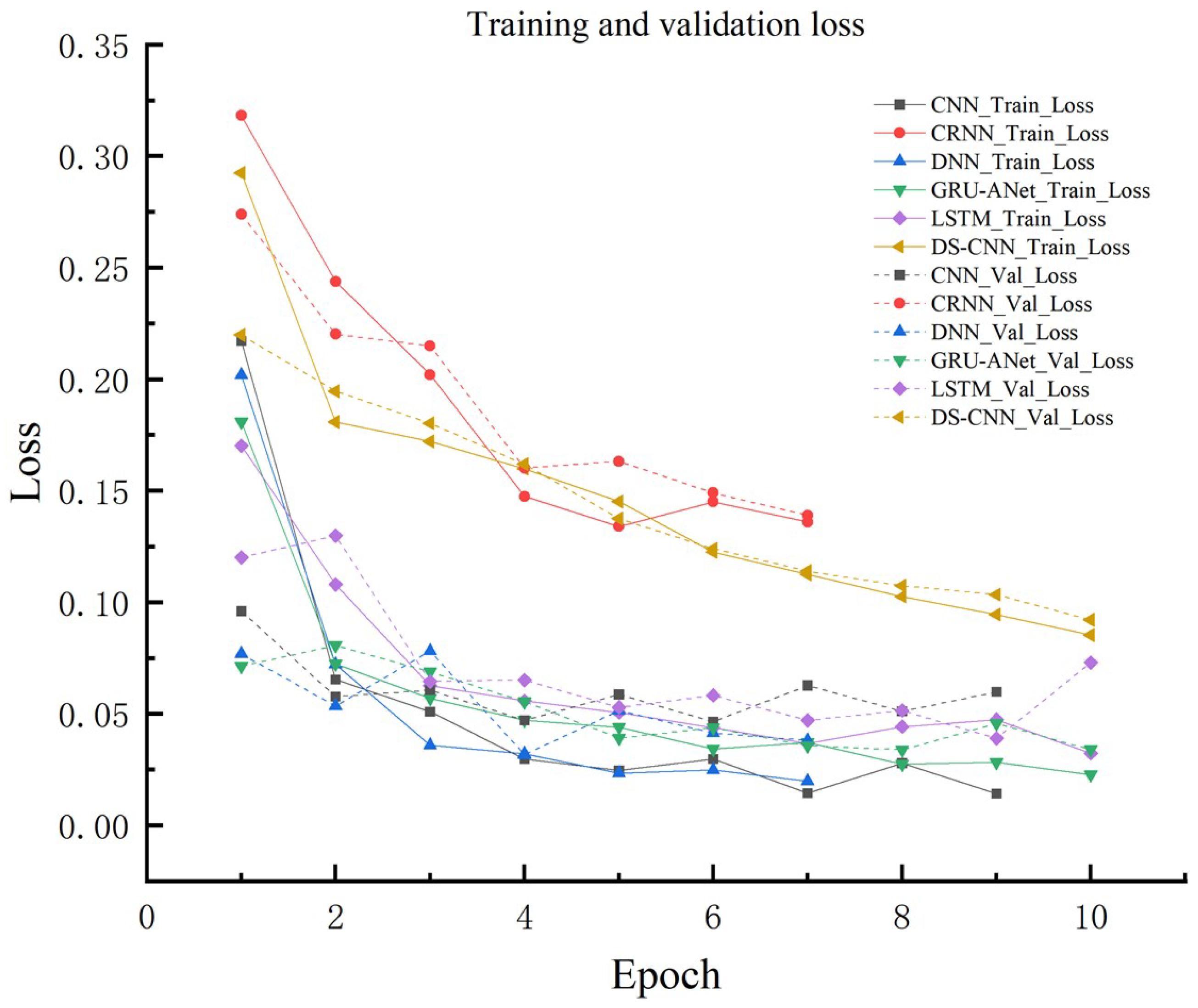
Figure 7.
Detection effect of different models on UAV acoustic signals.
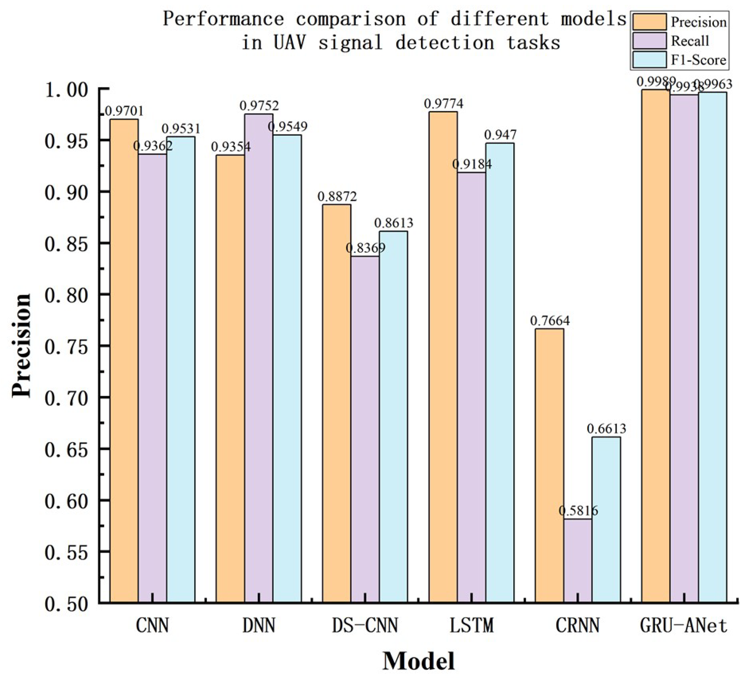
Figure 8.
Precision-recall curves.
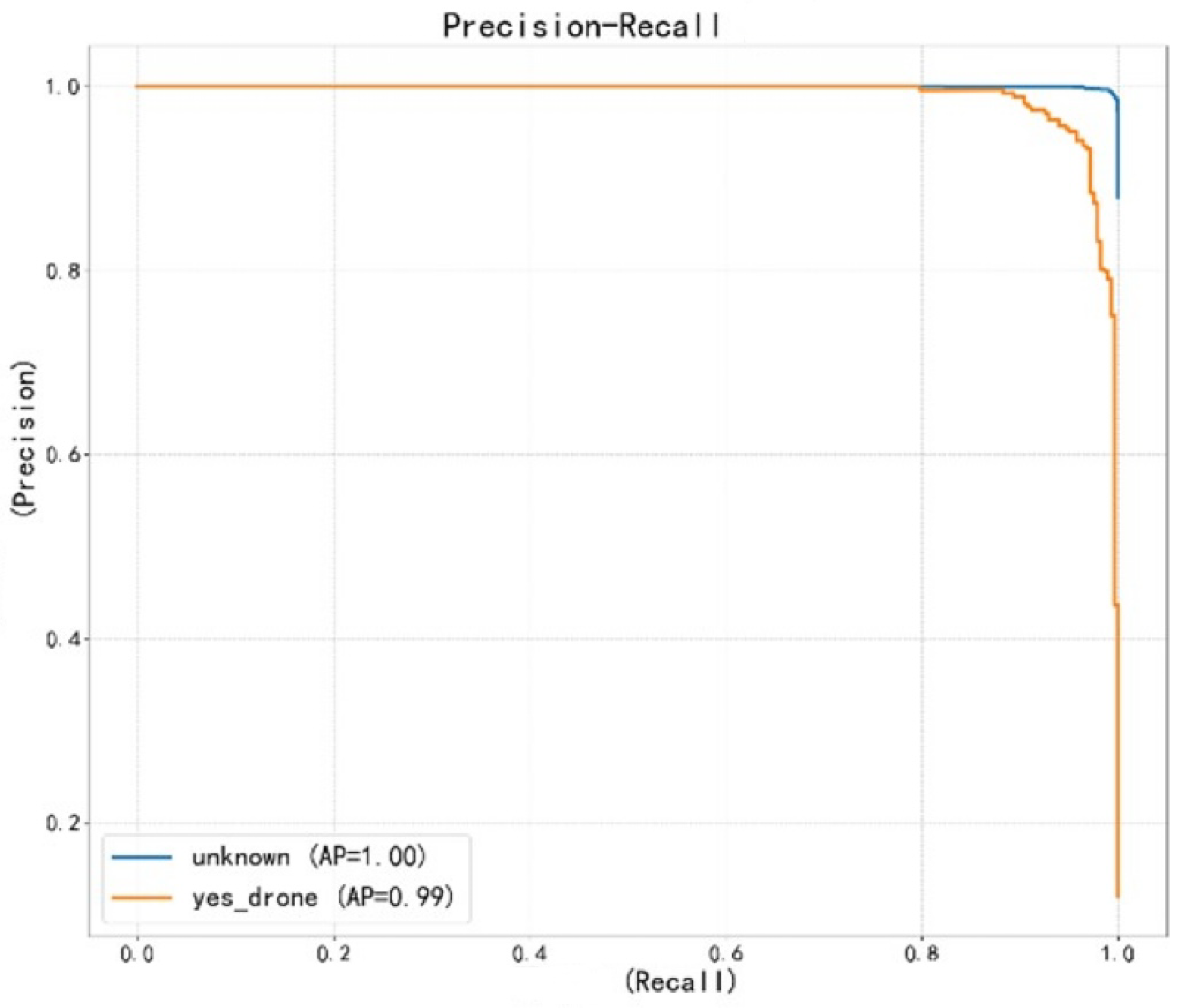
Figure 9.
Comparison of attentional mechanism ablation experiments.
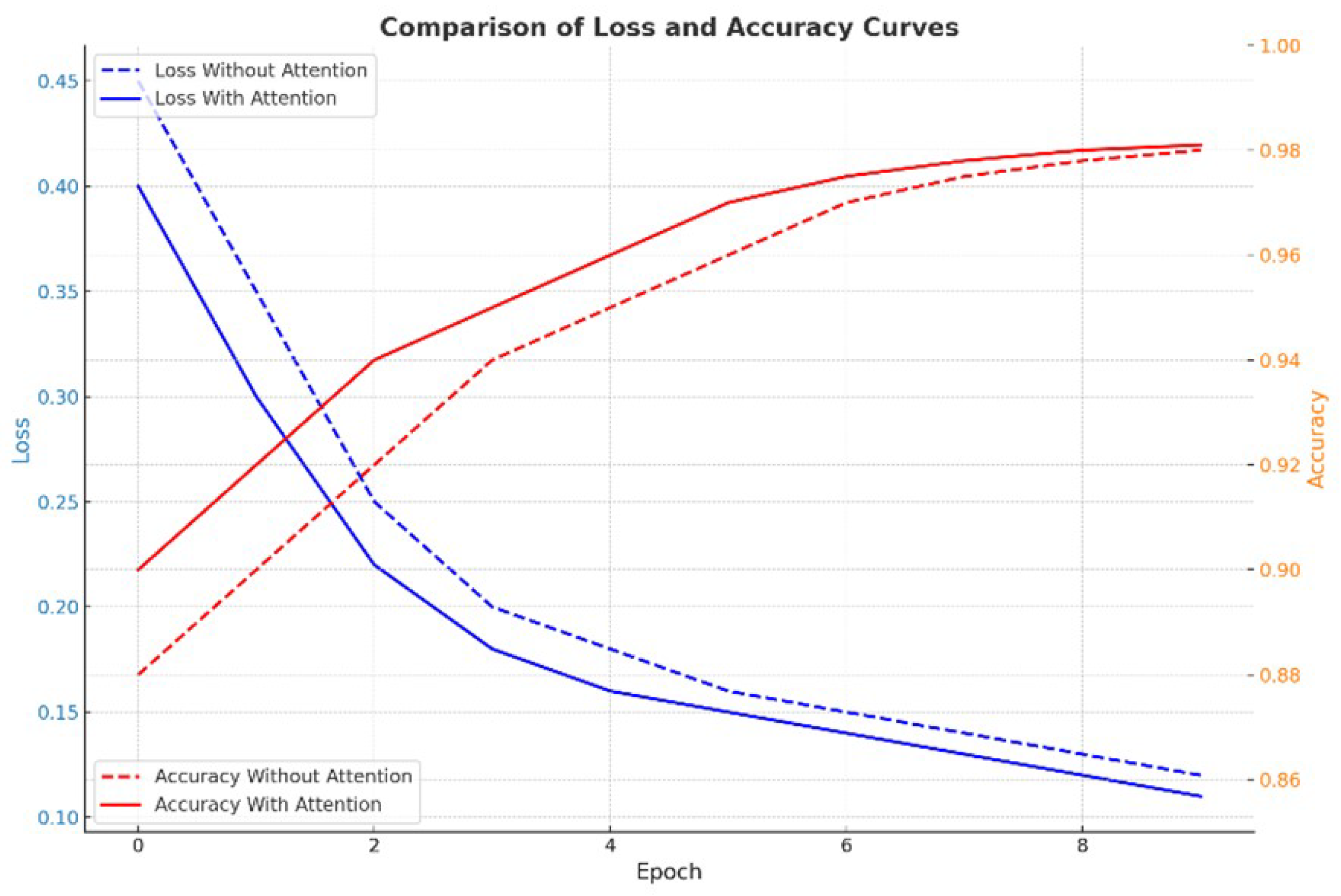

Table 1.
Comparison of reaction times.
| Model | Training time | Validation set processing time |
|---|---|---|
| CNN | 72s (10 epochs, 7.2s/epoch) | 1s |
| CRNN | 98s (7 epochs, 14s/epoch) | 1s |
| DNN | 56s (7 epochs, 8s/epoch | 2s |
| GRU-ANET | 60s (10 epochs, 6s/epoch) | 1s |
| LSTM | 65s (10 epochs, 6.5s/epoch) | 1s |
| DS-CNN | 60s (10 epochs, 6s/epoch) | 1s |
Disclaimer/Publisher’s Note: The statements, opinions and data contained in all publications are solely those of the individual author(s) and contributor(s) and not of MDPI and/or the editor(s). MDPI and/or the editor(s) disclaim responsibility for any injury to people or property resulting from any ideas, methods, instructions or products referred to in the content. |
© 2025 by the authors. Licensee MDPI, Basel, Switzerland. This article is an open access article distributed under the terms and conditions of the Creative Commons Attribution (CC BY) license (http://creativecommons.org/licenses/by/4.0/).
Copyright: This open access article is published under a Creative Commons CC BY 4.0 license, which permit the free download, distribution, and reuse, provided that the author and preprint are cited in any reuse.


