
Submitted:
12 February 2025
Posted:
14 February 2025
You are already at the latest version
Abstract
Ultrasonic TOFD imaging, as an important non-destructive testing method, has a wide range of applications in pipeline girths weld inspection and testing. Due to the limited bandwidth of ultrasonic transducers, near-surface defects in the weld are masked and cannot be recognized, resulting in poor longitudinal resolution. Affected by the inherent diffraction effect of scattered acoustic waves, defects image has noticeable trailing, resulting in poor transverse resolution of TOFD imaging, and making quantitative defect detection difficult. In this paper, based on the assumption of sparseness of ultrasonic defects distribution, by constructing a convolutional model of the ultrasonic TOFD signal, Orthogonal Matching Pursuit (OMP) sparse deconvolution algorithm is utilized to enhance the longitudinal resolution. Based on synthetic aperture acoustic imaging model, in wavenumber domain, back propagation inference is implemented through phase transfer technology to eliminate the influence of diffraction effects and enhance transverse resolution. On this basis, the time domain sparse deconvolution and frequency domain synthetic aperture focusing methods mentioned above are combined to enhance the resolution of ultrasound TOFD imaging. The simulation and experimental results indicate that this technology can outline the trend of defects with fine stripes and reduce the image resolution about 35%.
Keywords:
Ultrasonic imaging
; Time Of Flight Diffraction (TOFD)
; Sparse deconvolution
; Synthetic aperture focusing technique (SAFT)
; Imaging resolution enhancement
1. Introduction
Ultrasonic TOFD imaging, as an important imaging method for the pipeline girth welds nondestructive testing, uses diffraction time difference as the basic parameter for quantitatively detecting internal defects . It complements with the phased array zonal ultrasonic imaging method and can provide more precise defect distribution of girth welds. TOFD has become one of the most important methods for quantitative evaluation of weld quality at present, especially for the quantitative characterization of the size and burial depth of vertical crack defects inside the weld seam, it exhibits obvious technical advantages. However, this imaging method has always been affected by signal oscillations caused by the limited frequency band of the transducer and the inherent diffraction effect of defective echo scattering, resulting in unsatisfactory longitudinal and transverse resolutions, the existence of detection blind area, and insufficient detection accuracy. In addition, the real-time limitations of its time-domain imaging method seriously affect the detection performance and online application ability of this method. For this reason, classic deconvolution techniques such as parameterized inverse filtering [1,2], high-order spectral analysis (cepstral theory) [3], and L2 regularized norm reconstruction [4,5] have been applied, effectively improving the longitudinal resolution of ultrasound TOFD imaging.Nevertheless, there are still technical pain points such as low signal-to-noise ratio and low contrast ratio, and further requirements of resolution enhancement.
For improving lateral resolution, time-domain SAFT technology is mainly used [6,7] , which calculates the wave arrival delay between the transducer and the defect, and reconstructs the defect imaging target data through the delay and sum rule. The calculation process of this method is simple, but it requires point-to-point calculation of the imaging area, with limited accuracy and efficiency. TOFD has become one of the most important methods for quantitative evaluation of weld quality at present, especially for the quantitative characterization of the size and burial depth of vertical crack defects inside the weld seam, it exhibits obvious technical advantages [8,9]. However, this numerical reconstruction method requires repeated iterative computation, which brings heavy computational burden. Recently, frequency-domain SAFT methods, also known as wavenumber-domain SAFT, have been widely studied due to their high-quality imaging result and high computational efficiency. The performance of frequency-domain SAFT have been verified in different modes, such as monostatic ultrasonic imaging [10,11], total focusing method ultrasonic imaging [12,13], compound plane wave ultrasonic imaging [14,15], etc. However, this method is established on the foundation of specific ultrasonic imaging model, which is still not be studied in TOFD ultrasonic imaging.
Based on the above background, it is proposed to conduct research on online high-resolution ultrasound TOFD imaging technology for the pipeline girth welds. The proposed method improves the TOFD image resolution in both longitudinal and transverse directions with an extreme low time costs, providing a potential to realize real-time quantitative TOFD detection. According to the simulation and experimental results, the proposed method can outline the trend of defects with very fine stripes, and the transverse resolution of image is reduced about 35%. Also, the time cost of the proposed method is 0.96 second and much less than the TOFD data acquisition time, showing the potential for real-time inspection.
2. Theoretical Expression of the General Model for Ultrasound TOFD Imaging Detection Signals
Ultrasound TOFD imaging detection mainly includes five processes from emission to reception, which are ultrasonic transducer excitation, incident propagation, defect response, reflection propagation, and ultrasonic transducer reception respectively, as shown in Figure 1. According to the classical linear system theory, the general theoretical expression for the ultrasound TOFD detection signal is obtained as:
Among them, represents the recieved TOFD signal, and represent the exciting response function and recieving response function of the ultrasonic transducers respectively, and represent the time-spatial response functions of the incident propagation path and the received propagation path, represents the spatial distribution function which used to characterize the reflection response of the defect. Where, represents the detection position of the TOFD signals and denote the spatial position of the specific point in ROI. is also the reconstruction goal of high-resolution ultrasound TOFD imaging, and ⨂ represents the convolution operator.
Although all five processes mentioned above are correlated using convolution, their convolution dimension and method are different. and modulate signals in the time domain, and its convolution occurs in the time domain, mainly manifested in its effect on signal bandwidth. However, and are convolutions in the time spatial domain, which mainly represent the diffraction effect of ultrasound waves in physical space. Furthermore, Equation (1) can be separated into two separate parts and express it in the spatial frequency domain as:
As shown in Equation (2), the reflection coefficient function is separated out as an intermediate. The above two equations are the two problems addressed in this paper, where is calculated from the measured data , which mainly eliminates the problem of signal bandwidth degradation caused by the transducer response and improves the longitudinal resolution of TOFD imaging. In contrast, the use of to solve for eliminates diffraction effects and improves the lateral resolution of TOFD imaging. Of course the exact form of the solution will be adapted to the actual situation, but it is fundamentally a temporal and spatial enhancement of the image resolution in terms of the signal bandwidth and diffraction problem.
3. High Longitudinal Resolution Ultrasound TOFD Imaging Based on Sparse Deconvolution
3.1. Sparse Deconvolution Model for Ultrasound TOFD Signals
Due to the limitation of the bandwidth of the transducer, and the transmitted and received ultrasound waves have multiple periodic oscillations,resulting in decrement in the longitudinal (i.e. depth) resolution of TOFD imaging. These periodic oscillations can be modeled as the convolution of transducer’s the emission and reception electronic pulse responses which are irrelevant to physical space, the effect of spatial dimensions can be ignored when eliminating transducer response effectiveness, at this point, and can be treated as and . Here, we use the time-domain one-dimensional discrete convolutional model to represent Equation (2) in time domain:
In the formula, represent the recieved TOFD signal, and represent the overall response of the transducer’s emission and reception of electronic pulses, which can be expressed as . represent the reflection coefficient function of the acoustic reflector, and represent the noise.It should be noted that the above convolution operation constructs the incident reference signal with zero as the center reference point, and intercepts the first M vector dimensions after convolution as the representation of signal .Therefore, the vector dimensions before and after convolution operation are consistent. Equation (4) is a standard linear model of ultrasound imaging. Since only the defects reflect the ultrasound waves in TOFD imaging system, the reflection coefficient function p could be used to describe the defect information. Such a linear model also used for different ultrasound imaging techniques [16,17,18]. The electronic pulse response can be established through the testing frequency response characteristics of various electronic devices, or a set of large plane ultrasonic echo signals can be directly selected for measurement, because the large plane echo signals already approximate the information of ultrasonic signal periodic oscillation.
Obviously, the reflection coefficient function contain all the defect information of the object to be tested, and is not limited by the ultrasonic signal bandwidth with extremely high longitudinal resolution. Therefore, it is necessary to obtain the reflection coefficient function of the object to be tested, and solve it according to Equations (4) with known and . This process is called deconvolution. Due to the presence of noise in actual signals, there is not a strict convolutional relationship between TOFD signal, electronic pulse response, and reflection coefficient function. Directly performing deconvolution can easily lead to ill conditioned solution. To avoid the impact of noise on the solution results, the deconvolution process will be transformed into a linear equation solving approach. To construct the linear equation of Equation (4) , the Fourier transform matrix is introduced to perform the Fourier transform:
In the formula, is defined as the spectrum of electronic pulse response, while the Fourier transform matrix F is defined as:
Then, by diagonalizing the frequency spectrum of electron pulse response, a Toeplitz cyclic matrix can be constructed as:
In the formula, is used to balance the energy changes during discrete Fourier calculations, and † is a conjugate operator. The Toplitz cycle matrix has generalized diagonality, which can be seen as the spatial translation of the electron pulse response in the matrix . Obviously, multiplying vector and matrix yields the same result as performing truncated and equal length sum e convolution [5]. Therefore, the linear equation of Equation (4) is expressed as
In the formula above, is a square matrix . According to the least squares method, the solution in Equation (5) can be expressed as:
where represents the norm.
Theoretically speaking, when the noise level is not high or the condition number of the convolutional matrix is not large, using the least squares method can suppress noise partly and solve out the reflection coefficient function . The low noise level here is mainly manifested as signal-to-noise ratio greater than 0 dB, even higher than 12 dB. The condition number of convolutional matrix can be approximately understood in practical applications as the ultimate expected limit resolution of electronic pulse response. When constructing a convolutional matrix , the size of the translation interval depends on the the ultimate limit resolution. When the translation interval increases and the correlation between row and column vectors goes down to half of its own energy, the condition number satisfies the requirement of stable solvability. However, in practical applications, if the translation interval directly takes the discrete sampling interval, it will cause the correlation between row and column vectors to be much greater than half of its own energy, leading to ill-conditioned in equation solving. Meanwhile, Equation (9) use the norm as the optimization objective, which is similar to a Gaussian distribution, resulting in excessively smooth solution results and limited improvement in longitudinal resolution.
Usually, in the application environment of ultrasonic non-destructive testing, the probability of defects appearing is relatively very low, and their distribution has large sparsity, that is, the proportion of defect areas in the tested object is very small, independent and discrete. Therefore, a prior assumption of sparse distribution can be introduced into the reflection coefficient function of the tested object, which is to add a set of sparse constraints to the above optimization objective function and rewrite it as:
The norm in the above formula refers to the number of non zeros in , and this type of constraint method on the model is called regularization. Common regularization methods include constraints(Tikhonov regularization constraints), and constraints etc. The constraint term added here has a strong sparse constraint effect on , while trying to avoid ill-conditioned solutions caused by discomforting in the equation solving process. On the basis of correctly solving the defect position, it can effectively suppress the smoothing effect brought by the norm in Equation (10), and improve the longitudinal resolution of ultrasound TOFD imaging as much as possible.
3.2. Sparse deconvolution optimization method for ultrasound TOFD signals
Based on the linear equation model of Equation (10), multiple optimization methods can be used to solve it, which include common algorithms such as base pursuit (BP) [10,11,12] and match pursuit (MP) [13,14,15] , but their solution approaches are vastly different. The BP algorithm can be seen as a subtraction operation, which projects the echo signal into a new space through the inverse mapping of the matrix . In this space, the defect energy is concentrated and the amplitude is amplified, while the noise energy is dispersed and the amplitude is reduced. Therefore, during the iterative process of solving, the main energy is retained by gradually eliminating the excess small amplitude components, thus achieving the goal of sparse reconstruction. Due to the need for the Jacobian matrix or Hessian matrix of linear equations in the BP calculation process, the solving process still relies on convex optimization theory, which has certain limitations on the model and is not compatible with norm constrained problems. The MP class methods are mainly based on greedy algorithms [16], similar to incremental operations. After initialization, they are set to zero vectors and continuously add non-zero terms during iteration to approximate the optimization results. Compared to other methods, for ultrasound TOFD detection, solving targets based on norm constraints is more suitable for optimization using MP class algorithms. Thus, the Orthogonal Matching Pursuit (OMP) algorithm [17] will be used to solve Equations (7) . Before introducing OMP, the conventional MP algorithm will be introduced, and its main process is as follows:
STEP 1: establish dictionary codebook , stimulating atomic libraries , residual , sparsity K, iterative counter ;
STEP 2: if
①: calculate degree of relevance:
②: select optimal atoms:
③: update residuals:
④: next: , goto STEP2;
, else goto STEP3;
STEP 3: end the loop and get the result: .
In the initialization process, the dictionary codebook is a sparse spatial mapping matrix. In ultrasonic non-destructive testing, the reflection coefficient function itself has sparsity, at the same time, the matrix has cyclic traversal characteristic. Therefore, the codebook can be directly replaced by convolutional matrices . In correlation calculation, the atom with the highest correlation is calculated by the inner product between the estimated residuals and the codebook. Then, the atom with the highest degree of relevance is selected and entered into the excitation atom library. Meanwhile, the residual value is updated, and this cycle is repeated until the sparsity counter is satisfied.
The dictionary codebook mentioned here is actually a set of basis . If this set of basis is orthogonal, then:
It can be seen that when the codebook is an orthogonal basis, can be directly mapped to . Therefore, it is reasonable to represent the main sparse components by selecting several points with the highest degree of relevance in the vector . Typically, the codebooks are redundant basis, and their redundancy degree depends on the condition number of the convolutional matrix , this leads to non-linear mapping relationship between and . To eliminate the difference between and caused by the correlation between redundant basis, it is necessary to orthogonalize the matching pursuit using OMP (Orthogonal Matching Tracking) method [20].
The orthogonalization of OMP is achieved by eliminating the correlation between vectors within redundant basis, and achieves more accurate matching. The basic process of OMP is similar to MP, with slight differences in correlation calculation [21]. Assuming there are already k atoms, and the normalized basis vectors corresponding to these excited atoms in the codebook are denoted as . In order to eliminate the impact of non orthogonality of each vector in the redundant basis, the new normalized basis vector is modified during the next round of correlation calculation:
where is the normalized vector basis corresponding to the selected atom in the next iteration in the Equation (12). Obviously, Equation (12) can achieve the normalized vector to be continuously reconstructed during the iteration process, forming an effect similar to orthogonal basis to ensure the accuracy of sparse imaging as much as possible.
The entire OMP calculation has a hyperparameter, which is the sparsity K, and the selection of sparsity K needs to be determined based on the actual object of ultrasonic testing. For ultrasound TOFD, each A-scan signal will contain lateral wave and backwall reflection wave, so at least two atoms of need to be represented. In the case of defect presence, there will also be diffraction waves at the defect tips. Due to the independent and discrete sparse distribution of defects, it is considered that there is only one set of defects in single A-scan signal at the same time. Therefore, setting the K value to 3 or 4 is more appropriate. It should be noted that in subsequent experiments, the lateral wave is truncated and omitted after straightening, so its sparsity K is correspondingly decreased by 1.
4. High Transverse Resolution Ultrasound TOFD Imaging Based on Frequency Domain SAFT
The scanning imaging process of ultrasonic TOFD for pipeline girth welds is actually a D-scan which moves along the girth direction. The transducers are symmetrically arranged on both sides of the weld seam, and driven by a mechanical device. In an ideal situation, when the acoustic axis of the transmitting transducer passes through a defect, an extremely strong reflected echo will be generated and captured by the receiving transducer for detecting the target defect.However, in practical applications of TOFD, the directionality of sound waves is not like that of lasers, but rather generates diffraction at the defect tips, forming arc-shaped reflected waves. Therefore, even point defects can be detected by probes at multiple locations, forming a "tail" shaped curved defect image. For continuous long strip cracks, there are obvious trailing arcs at both ends of the crack, which can easily lead to inaccurate judgment of defect size and burial depth.
To solve the problem of reduced transverse resolution mentioned above, it is often necessary to use Synthetic Aperture Focusing (SAFT) [16,22] technology to reconstruct images. However, the D-scan image of TOFD is different from conventional two-dimensional B-scan images, its essence is to project three-dimensional spatial information into two-dimensional images, which will inevitably lead to certain information lossness. The most direct explanation example is that D-scan only collects one A-scan line on each axial section and estimates the defect position based on the time delay of reference echo. However, for the same echo time delay, there are multiple possible defect positions on its axial section, and its specific position information cannot be determined. Usually, the SAFT technique for TOFD imaging approximates the central imaging assumption of defects, assuming that the defects are located at the centerline position of the transducer pair. When the defect is assumed to fall on the centerline of the transducer pair, the emission and reception processes of sound waves naturally satisfy the condition of symmetrical sound path, that is, the emission path and reception path are symmetrical about the centerline.
According to Equation (1), the spatial diffraction propagation process of ultrasound TOFD can also be constructed by a convolutional model, which is usually defined in the analytical model as a finite amplitude Delta signal with amplitude information . As shown in Equation (3), the convolution model can be simplified by multiplying the transmitting frequency-spatial function , the amplitude information and the receiving frequency-spatial fucntion in frequency domain. In order to associate the angular frequency with the propagating direction of the ultrasonic waves, is replaced with the wavenumber . Thus Equation (3) is rewritten as
The imaging reconstruction is the inverse computation process of from . Neglecting the multiple reflections of sound waves in propagating process, the transceiver path is symmetry. Thus, the frequency-spatial functions for transmitting and receiving are equalvalent without differences
Since can be regarded as the 2-D free-space Green’s function , Equation (13) is then obtained as
In TOFD, the transmitting and receiving probes are symmetrically distributed on both sides of the weld. Therefore, the processes of wave incident onto central weld defects, and wave scattering from the defects and received by receiver are also symmetrical. To simplify the calculation of symmetrical bidirectional wave field propagation, the Explosion Reflection Model (ERM) is introduced. Under ERM, we assume that the sound speed of the propagating medium is half of its real value (cerm=c/2), and the propagation process can be equivalently modeled as ultrasonic waves being autonomously emitted from each pixel point, which are then received by the ultrasonic transducer. The phase information of the sound waves is consistent with the self-emission and reception scenario, and the waveform is equivalent along the time axis. In this model, all scatter points are set to emit sound waves at the same time—referred to as the “explosion” moment—and their intensity is directly proportional to the reflection coefficient of each point. The sound fields produced by these points are emitted simultaneously and received together by the ultrasonic transducer. This simplifies the bidirectional wave propagation and only considers the sound field received from the upward returning probe.
According to Weyl’s integral, the Green’s function in the 2-D free space can be expanded and expressed as:
It can be seen that the relationship between and established by Equation (17) has a complex Fourier decomposition relationship, and here we perform an inverse Fourier transform over . Equation (17) can be rewritten as:
For convenience, we assume that when the size of ROI remains unchanged in the depth direction. Similarly, the amplitude information can be replaced by the spectrum through a Fourier transform over x
According to the analysis based on plane wave model, the acoustic phase has a much larger modulation effect on the signal than , and thus can be neglected here. Since the final image can be normalized, the constant coefficient is also discarded. Equation (19) is simplified as
Equation (20) can be replaced with recursive formula
where is the wavenumber along the z-axis. The whole process of wavefield derivation is to calculate and thus estimate the defect signal with the given wavefield . However, unlike the conventional B-scan, the deduced depth information z of D-scan is not directly equal to the defect depth, and because of the lateral distance PCS between the transducer’s scanning plane and the imaging plane, the deduced depth should be corrected as follows:
Its corresponding derivation formula should be written as
The amplitude information is calculated by performing an inverse Fourier transform over . Since the actual signals is band limited, then the final image is obtained by superimosing all the values over the wavenumber as
In summary, the high lateral resolution is obtained with the following calculation steps
The longitudinal resolution optimized data is written as , where is equal to . is calculated with the sparse deconvolution for each position as
The Fourier transform matrix over is defined as
The following recursive wavefield derivation at depth z is to left multiply the dispersion relation matrix
The inverse Fourier transform matrix over is defined similarly as
The superimposition over is to right multiply the constant matrix as
The calculation of the final image at depth z is calculated with the aforementioned matrixed as
where ⊙ is the symbol of Hadamard matrix multiplication. The wavefield calculation for is then performed for each depth.
The entire computational workflow, depicted in Figure 2, primarily consists of three steps: frequency domain spatial mapping, phase migration, and imaging spatial inverse mapping. In the frequency domain spatial mapping step, a two-dimensional Fourier transform is employed to map the received signal into , with a computational complexity of approximately . The phase migration step involves extrapolating the mapped wavefield layer by layer to gather acoustic field information at different depths. The core computational step of this process is accomplished using the Hadamard product, resulting in a complexity of . The overall computation complexity is for the case of N imaging depth layers. The final step, imaging spatial inverse mapping, is conducted through the imaging condition formula, with a complexity of . When combining these three steps, the computation for the entire imaging reconstruction is , which is evidently more efficient than the required by traditional SAFT.
5. Ultrasound TOFD Imaging with Both High Longitudinal and Lateral Resolutions
Since the process of improving the longitudinal and lateral resolutions is holistic, we unify the two procedures as a whole. The acquired raw data is denoted as , where is equal to . First, the optimized data containing all the scanning positions is calculated in order to improve the longitudinal resolution. Second, the lateral resolution is improved with the frequency domain SAFT and then the final image is achieved. The whole process can be written as
where M represents the maximum depth in the final image.
6. Simulation and Experimental Research
In order to verify the effectiveness of the above method, simulation and experimental studies are carried out, and the design drawings and physical photographs of the specimen used are shown in Figure 3. The specimen is a flat plate butt-welded, and the inside of the weld contains five types of defects such as open transverse cracks, unfused bevels, root under-welding, longitudinal cracks and slag entrapment, and the thickness of the plate is 21 mm.
6.1. Simulation
The data generation for the simulation is based on the simulation software CIVA. The transceiver TOFD transducer with a diameter of 6 mm, center frequency of 5 MHz, bandwidth of 70% (-6 dB) is selected, wedge refracting angle is , Probe Center Separation(PCS) is 48.5 mm, scanning interval is 0.5mm, and transmitting transducer and receiving transducer are symmetrically arranged on both sides of the weld. At each scanning position, data is recorded with sampling rate , and as a result, each A-scan line data has a 500 points. The whole scanning step is 80 steps. The collected simulation data is a 80 × 500 matrix, and forms the D-scan TOFD image shown in Figure 4.
Due to the diffraction effect of ultrasound waves, the tips of defects presents arc-shaped artifacts, which can easily cause errors in the judgment of defect size and burial depth. For this reason, the above proposed frequency-domain synthetic aperture and sparse deconvolution methods are fused to realize the acoustic reconstruction of the D-scan TOFD imaging, results shown as Figure 5. The figure shows that the spatial resolution of ultrasonic TOFD imaging has been greatly improved, which lays a good foundation for the quantitative detection of annular weld defects in terms of size and embedment depth, but it should be noted that the weaker transverse crack signals are easily rejected after the above processing.
6.2. Experimental Studies
The specimen used in the experiment is consistent with those used in the simulation, with a V-type groove welded by argon-arc welding and manual electric-arc welding modes, and 5 sets of artificial defects are embedded same as the simulation. TOFD transducers are same to used in the simulation too, PCS is 48.5mm. These two transducers are tightly pressed against the steel specimen through a mechanical spring-compression device, and water is used to couple between the wedge and the steel plate. The scanning is controlled by a robotic arm, with a step accuracy of 0.5mm. The original imaging result of the scanning is shown in Figure 6.
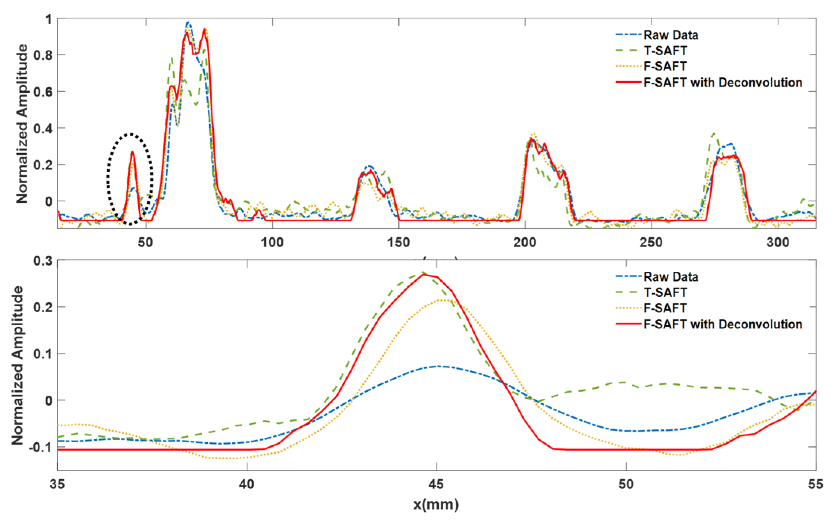
The time-domain and frequency- domain synthetic aperture focusing imaging are shown in Figure 7 and Figure 8 respectively, which shows that in the unwelded portion of the root, the frequency domain imaging method have a higher imaging contrast and can separate the defects from the bottom echo. At the same time, the combination of sparse deconvolution and frequency domain synthesized aperture can further improve the longitudinal resolution, and as shown in Figure 9, except for the transverse defects are difficult to identify, the longitudinal resolution of the other four defects can be greatly improved, so that the depths of defects can be clearly located as show in Figure 10. In Figure 11, the maximum intensity projection of each defects shows the improvements of transverse resolutions. Especially, in the localized zoomed in image, it can be seen that the full width at half maximum (FWHM) of the defects in raw data image, image reconstructed by time-domain SAFT, image reconstructed by frequency-domain SAFT and image processed by prosed method are 7mm, 5mm, 5mm and 4.5mm respectively. The proposed method can reduce transverse resolution about 35% comparing with raw data and better than 28% for traditional method. Moreover, the noise level of image reconstructed by proposed method is nearly decreased to zero. Thanks to the reduction of the computational volume of the frequency domain synthetic aperture technology, for the 300 ×1000-point TOFD signal data, the synthetic aperture reconstruction process takes about 0.1s, even if the frequency domain synthetic aperture and sparse inverse convolution fusion reconstruction takes about 0.96s, the reconstruction time is less than the sweeping data acquisition time, which meets the needs of on-line imaging inspection applications.
7. Conclusions
In this paper, an ultrasonic TOFD imaging enhancement technology for pipeline grith welds is proposed. This enhancement aims to use the reflection coefficients to image the defects. The reflection coefficients could be solved by eliminating the electrical and spatial pulse responses with sparse deconvolution and frequency-domain synthetic aperture focusing, respectively. Benefiting from the Fast-Fourier Transform, the enhancement process in frequency domain extremely reduces the computational time consumptions. The simulations and experiments demonstrated that using reflection coefficient representing the defects in image could significantly improve both the image longitudinal and transverse resolutions, which is advantage to point out the defect positions accurately. As a result, the proposed method could image the defects with high accuracy and efficiency.
This Work is Supported by Science Foundation of Donghai Laboratory (Grant No. DH-2022ZY0011).
References
- Besson, A. G. J. , Roquette, L., Perdios, D., etc. Fast Non-stationary Deconvolution in Ultrasound Imaging. IEEE Transactions on Computational Imaging, 2018, 7, 935–947. [Google Scholar]
- Zhouye Chen, Adrian Basarab, Denis Kouamé.Enhanced ultrasound image reconstruction using a compressive blind deconvolution approach. 2017 IEEE International Conference on Acoustics, Speech and Signal Processing (ICASSP), New Orleans, LA, USA, 05-09 March 2017.
- ABEYRATNE U R, PETROPULU A P, REID J M.. Higher order spectra based deconvolution of ultrasound images. IEEE transactions on Ultrasonics, Ferroelectrics, Frequency Control, 1064.
- CHEN Z, BASARAB A, KOUAMé D. A simulation study on the choice of regularization parameter in L2-norm ultrasound image restoration. In proceedings of the 2015 37th Annual International Conference of the IEEE Engineering in Medicine and Biology Society (EMBC), Milan, Italy, 25-29 August 2015.
- C. Sumi, T. Ou, J. Takishima, S. Shirafuji. Considerations about L2- and L1-norm regularizations for ultrasound reverberation characteristics imaging and vectoral Doppler measurement. 2022 44th Annual International Conference of the IEEE Engineering in Medicine & Biology Society (EMBC), Glasgow, Scotland, United Kingdom, 11-15 July 2022.
- SPIES M, RIEDER H, DILLHöFER A, et al. Synthetic aperture focusing and time-of-flight diffraction ultrasonic imaging—past and present. Journal of Nondestructive Evaluation, 2012; 31, 310–323.
- Chengyang Huang; Francesco Lanza Di Scalea. Application of Sparse Synthetic Aperture Focusing Techniques to Ultrasound Imaging in Solids Using a Transducer Wedge. IEEE Transactions on Ultrasonics, Ferroelectrics, and Frequency Control, 2023; 71, 280–294.
- LIU H, XIA H, ZHUANG M, et al. Reverse time migration of acoustic waves for imaging based defects detection for concrete and CFST structures. Mechanical Systems Signal Processing 2019, 117, 210–220. [Google Scholar] [CrossRef]
- RAO J, SAINI A, YANG J, et al. Ultrasonic imaging of irregularly shaped notches based on elastic reverse time migration. NDT & E International 2019, 107, 102135. [Google Scholar]
- Wolf, M. , Nair, A. S., Hoffrogge, P., etc. Improved failure analysis in scanning acoustic microscopy via advanced signal processing techniques. Microelectronics Reliability, 2022, 138, 114618. [Google Scholar] [CrossRef]
- Yu, B. , Jin, H., Mei, Y., etc. 3-D ultrasonic image reconstruction in frequency domain using a virtual transducer model. Ultrasonics , 2022, 118, 106573. [Google Scholar] [CrossRef] [PubMed]
- Jin, H. , Zheng, Z., Liao, X., etc. Image reconstruction of immersed ultrasonic testing for strongly attenuative materials. Mechanical Systems and Signal Processing, 2022, 168, 108654. [Google Scholar] [CrossRef]
- Jin, H. , Chen, J. An efficient wavenumber algorithm towards real-time ultrasonic full-matrix imaging of multi-layered medium. Mechanical Systems and Signal Processing, 2021, 149, 107149. [Google Scholar] [CrossRef]
- Merabet, L. , Robert, S., Prada, C. 2-D and 3-D reconstruction algorithms in the Fourier domain for plane-wave imaging in nondestructive testing. IEEE Transactions on Ultrasonics, Ferroelectrics, and Frequency Control, 2019; 66, 772–788. [Google Scholar]
- Merabet, L. , Robert, S., Prada, C. The multi-mode plane wave imaging in the Fourier domain: Theory and applications to fast ultrasound imaging of cracks. NDT & E International, 2020, 110, 102171. [Google Scholar]
- Chang, Z. , Xu, X., Wu, S., Wu, E., etc. (2024). Ultrasonic dynamic plane wave imaging for high-speed railway inspection. Mechanical Systems and Signal Processing, 2024, 220, 111672. [Google Scholar] [CrossRef]
- Su, L. , Tan, S., Qi, Y., etc. An improved orthogonal matching pursuit method for denoising high-frequency ultrasonic detection signals of flip chips. Mechanical Systems and Signal Processing, 2023, 188, 110030. [Google Scholar] [CrossRef]
- Gao, Y. , Mu, W., Yuan, F. G., etc. A defect localization method based on self-sensing and orthogonal matching pursuit. Ultrasonics , 2023, 128, 106889. [Google Scholar] [CrossRef] [PubMed]
- Mu, W. , Gao, Y., Liu, G. Ultrasound defect localization in shell structures with Lamb waves using spare sensor array and orthogonal matching pursuit decomposition. Sensors, 2021; 21, 8127. [Google Scholar]
- JIN H, YANG K, WU S, et al. Sparse deconvolution method for ultrasound images based on automatic estimation of reference signals. Ultrasonics, 2016; 67, 1–8.
- Wei Chen, Binghui Peng, Grant Schoenebeck, and Biaoshuai Tao. Adaptive Greedy versus Non-adaptive Greedy for Influence Maximization. Journal of Artificial Intelligence Research, 2022, 74, 303–351. [Google Scholar] [CrossRef]
- L. Peralta, A. L. Peralta, A. Gomez, Y. Luan, B. -H. Kim, etc. Coherent Multi-Transducer Ultrasound Imaging. IEEE Transactions on Ultrasonics, Ferroelectrics, and Frequency Control, 2019; 66, 1316–1330. [Google Scholar]
Figure 1.
The propagation process of ultrasound waves in TOFD imaging.
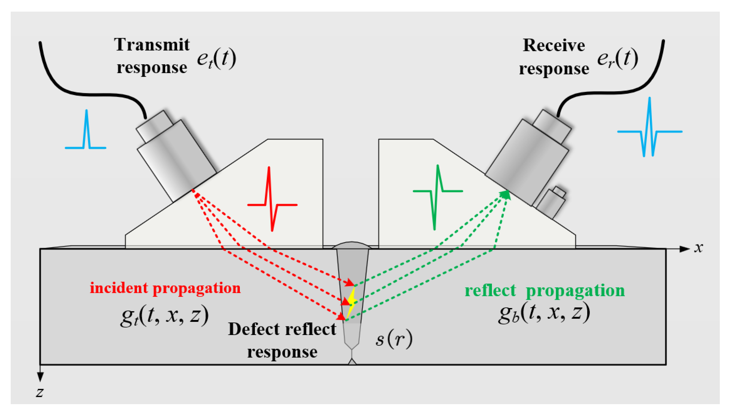
Figure 2.
Frequency-domain SAFT reconstruction process for TOFD-Dscan images and its computational complexity in each step.
Figure 2.
Frequency-domain SAFT reconstruction process for TOFD-Dscan images and its computational complexity in each step.
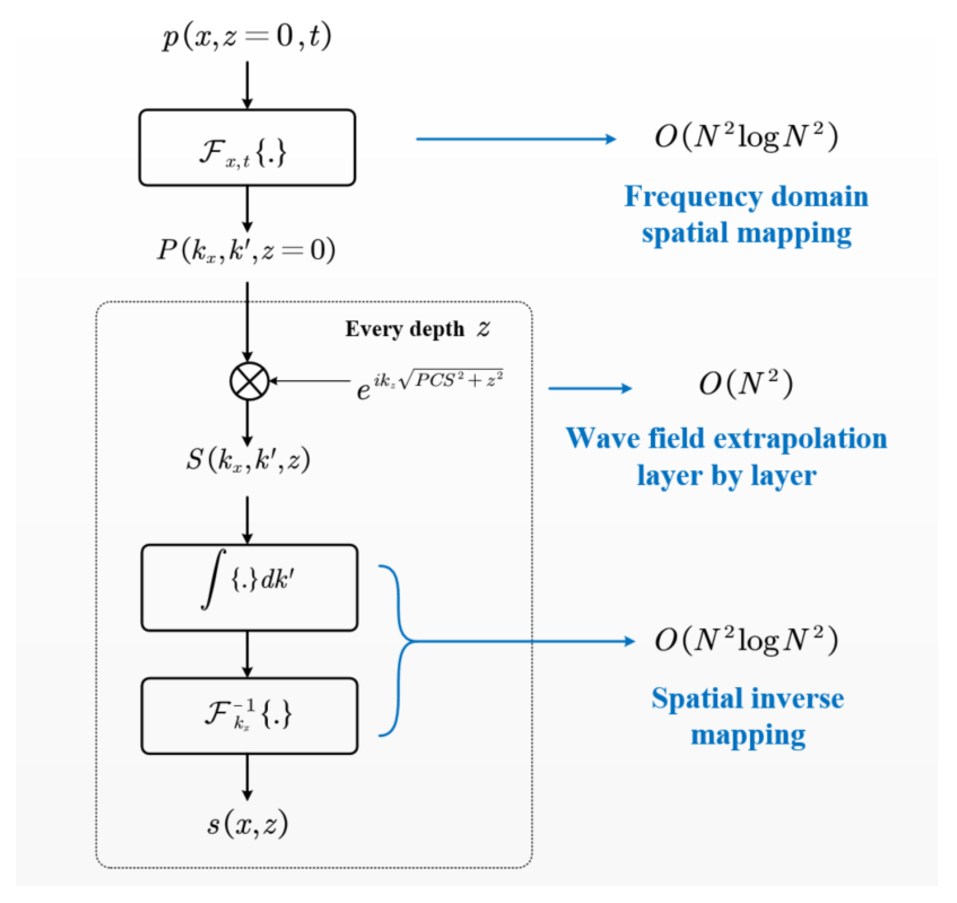
Figure 3.
V-bevel weld specimens with artificial defects.
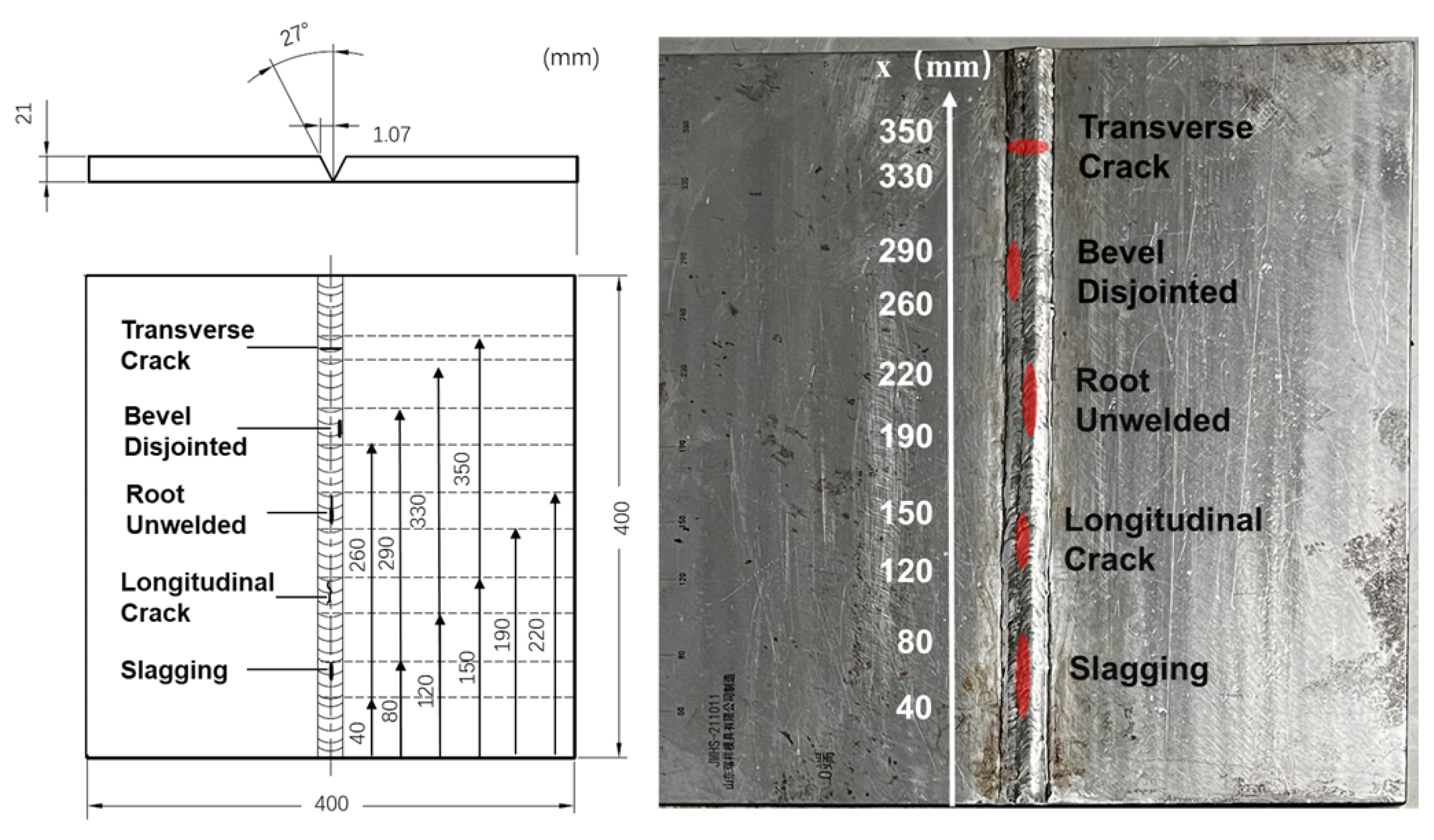
Figure 4.
Simulated images generated from raw data.
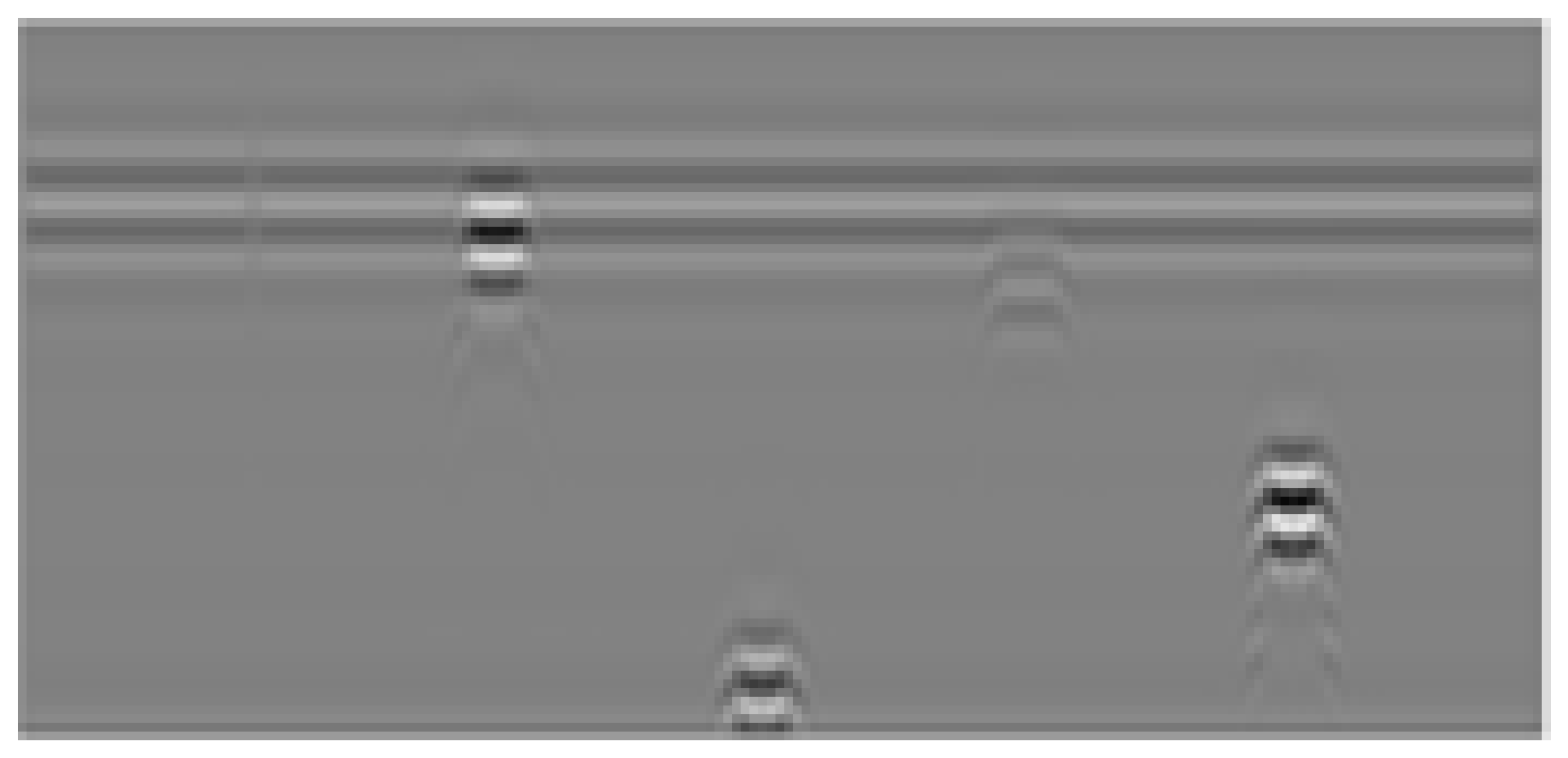
Figure 5.
Reconstruction results of the frequency domain synthetic aperture and inverse convolution fusion method proposed in this paper.
Figure 5.
Reconstruction results of the frequency domain synthetic aperture and inverse convolution fusion method proposed in this paper.
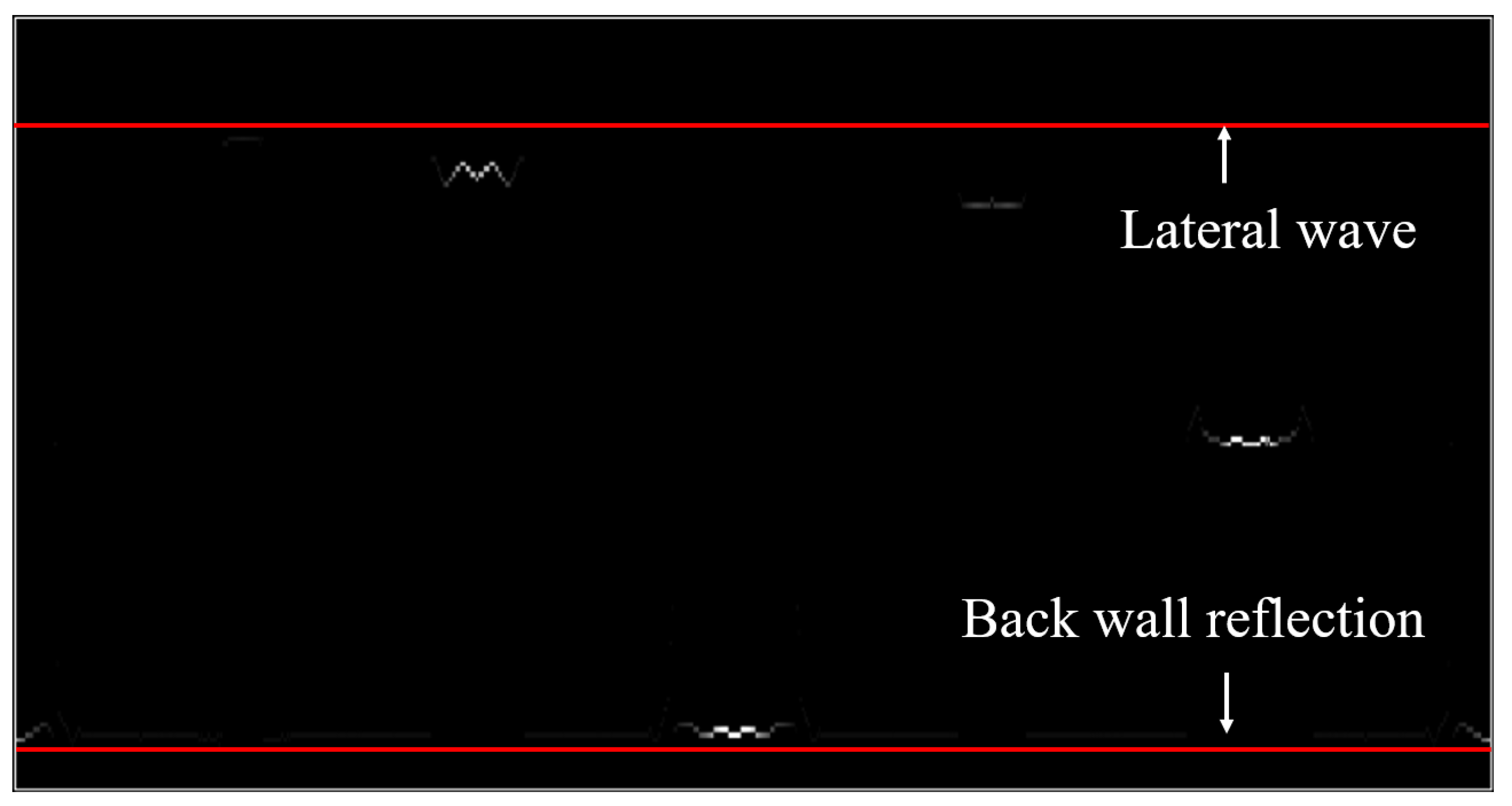
Figure 6.
Raw data imaging results.
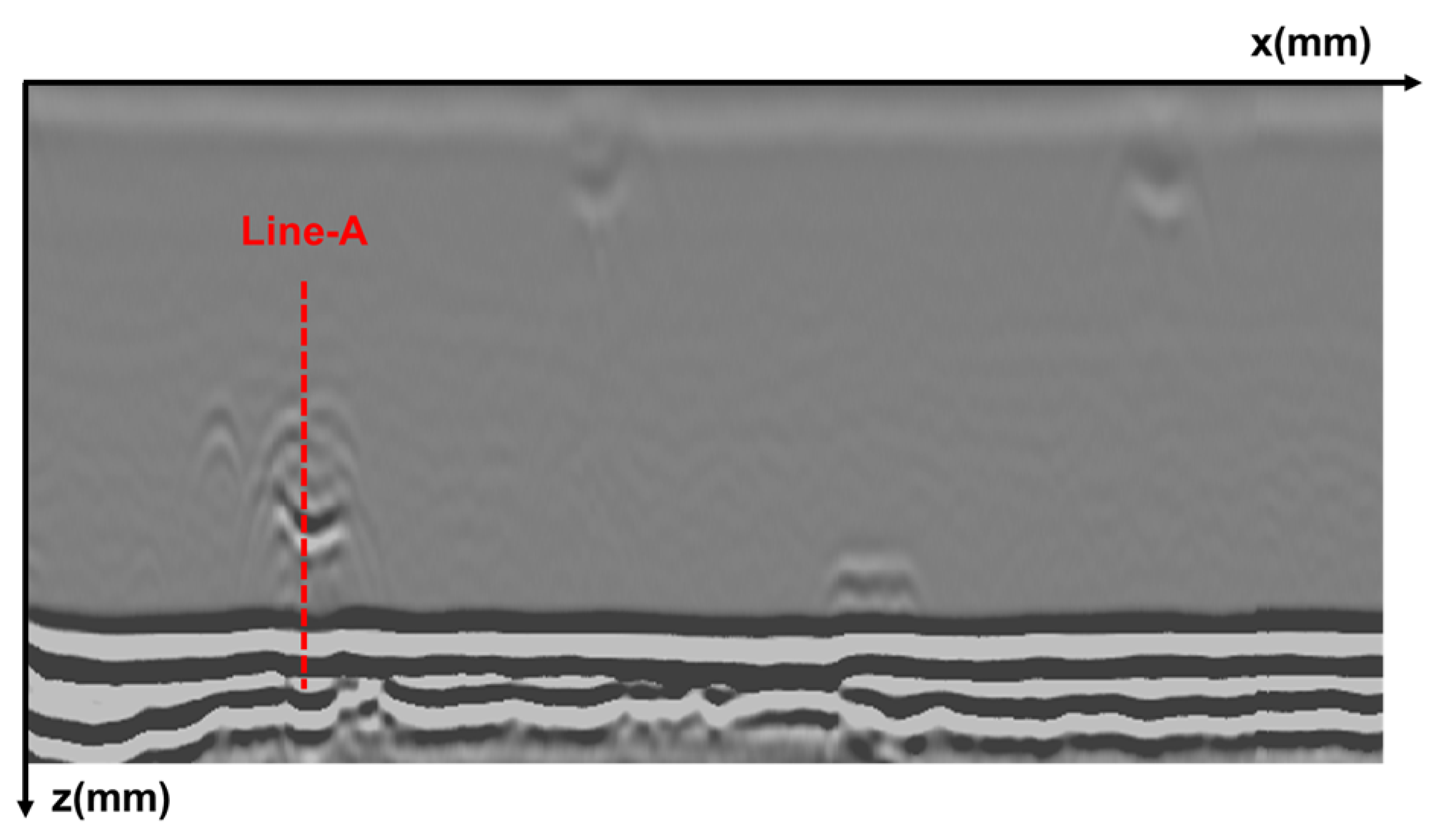
Figure 7.
Reconstruction results of time-domain synthetic aperture.
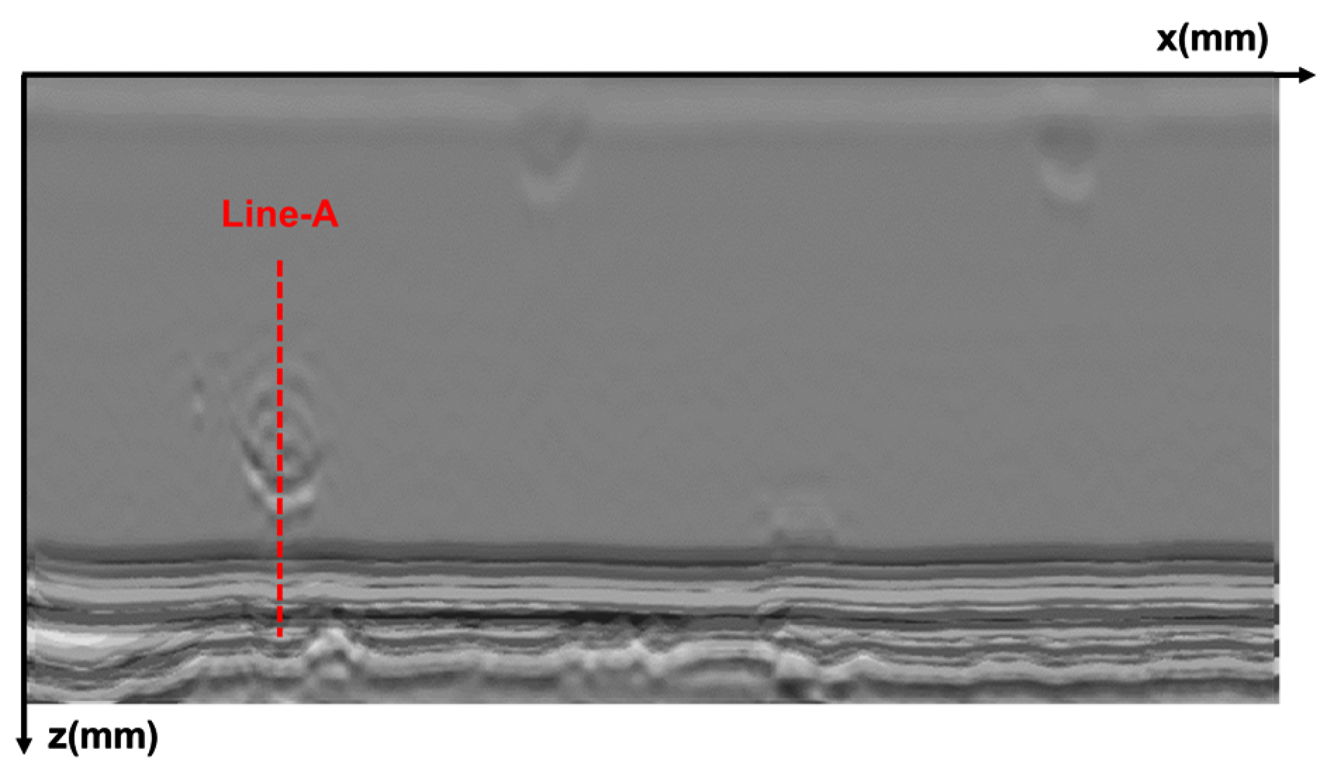
Figure 8.
Reconstruction results of frequency-domain synthetic aperture.

Figure 9.
Reconstruction results of frequency-domain synthetic aperture fused with sparse inverse convolution.
Figure 9.
Reconstruction results of frequency-domain synthetic aperture fused with sparse inverse convolution.
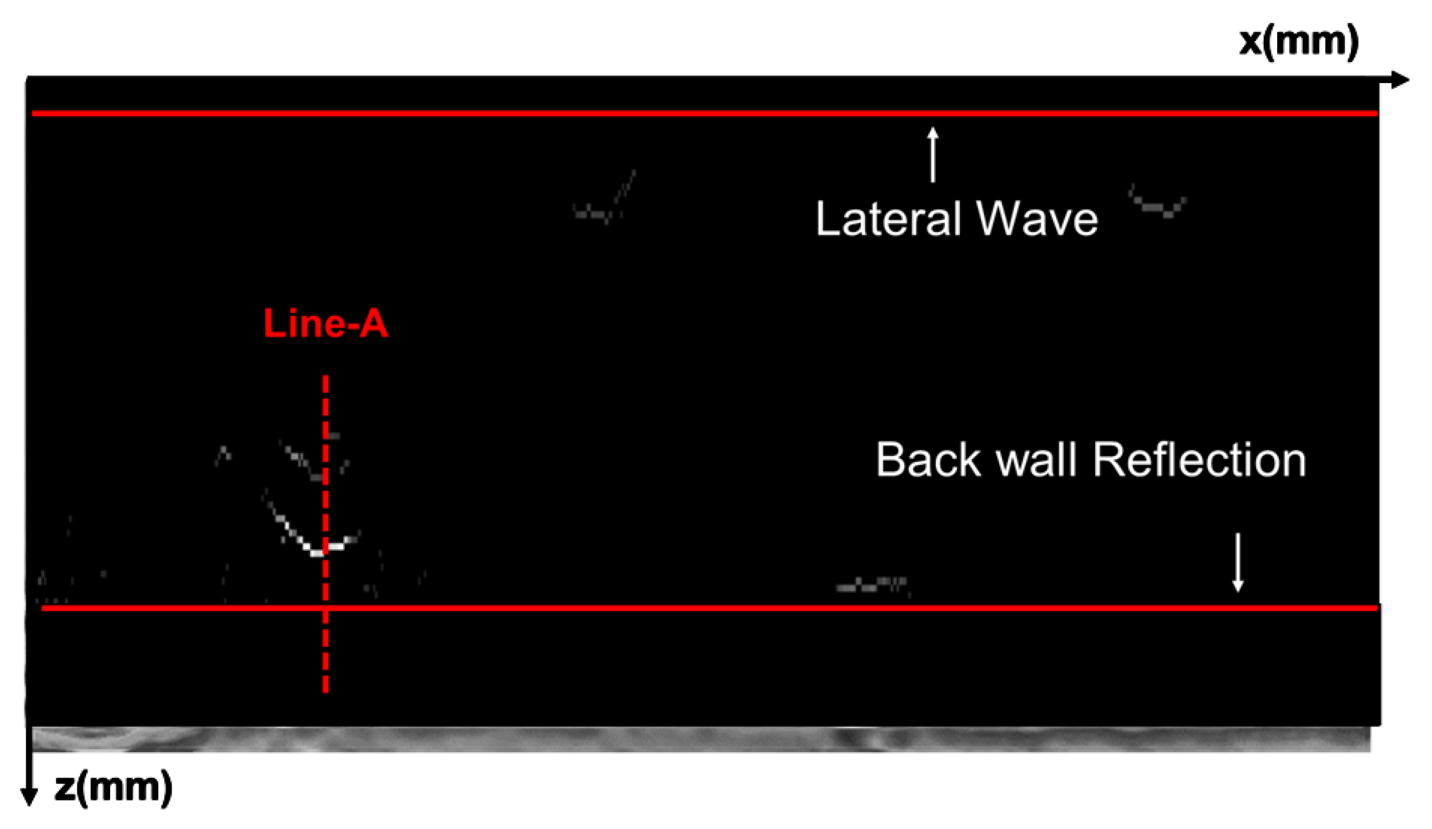
Figure 10.
The waveform at Line-A.
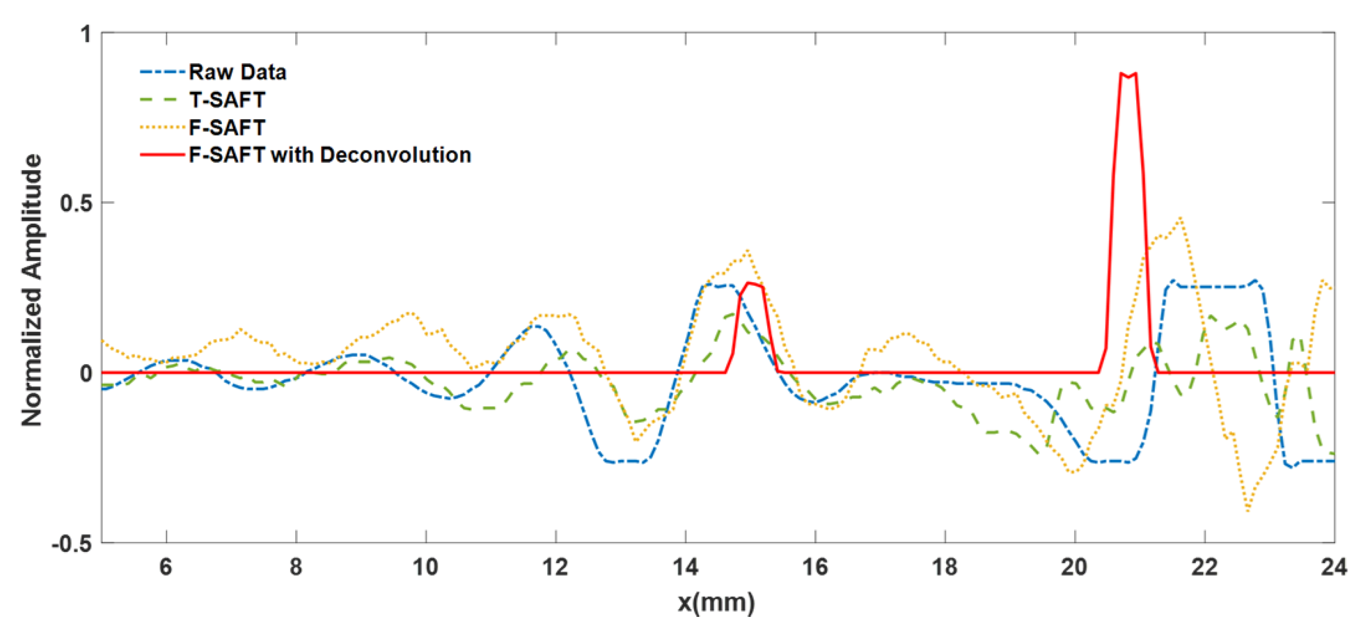
Figure 11.
The resolution analysis of imaging results. upper: The maximum intensity projection of defects; lower: Localized zoomed-in image of slagging defect..
Figure 11.
The resolution analysis of imaging results. upper: The maximum intensity projection of defects; lower: Localized zoomed-in image of slagging defect..
Disclaimer/Publisher’s Note: The statements, opinions and data contained in all publications are solely those of the individual author(s) and contributor(s) and not of MDPI and/or the editor(s). MDPI and/or the editor(s) disclaim responsibility for any injury to people or property resulting from any ideas, methods, instructions or products referred to in the content. |
© 2025 by the authors. Licensee MDPI, Basel, Switzerland. This article is an open access article distributed under the terms and conditions of the Creative Commons Attribution (CC BY) license (https://creativecommons.org/licenses/by/4.0/).
Copyright: This open access article is published under a Creative Commons CC BY 4.0 license, which permit the free download, distribution, and reuse, provided that the author and preprint are cited in any reuse.


