Submitted:
12 February 2025
Posted:
13 February 2025
You are already at the latest version
Abstract
The Baltic Sea is an intercontinental marginal sea that is vertically stratified with a strong halocline isolating the saline bottom layer from the brackish surface layer. The surface layer is eutrophic and abiotic zones lacking oxygen are common in the deeper regions. While freshwater is constantly flowing into the North Sea, oxygen-rich bottom waters can only occasionally enter the Baltic following a special sequence of transient weather conditions. These so-called Major Baltic Inflow events can be monitored via the sea level gradients between the Kattegat and the western Baltic Sea. Innovative interferometric altimetry from the Surface Water and Ocean Topography (SWOT) mission give us the first opportunity to directly observe the sea level signal associated with the inflow in December 2023. In addition, we use observations from recent high-rate multi-mission nadir altimetry. For scales larger than 50 km, SWOT and nadir altimetry are in very good agreement. The SWOT observations are compared to the simulations with the regional 3D HBMnoku ocean circulation model operated by the German Federal Maritime and Hydrographic Agency (BSH). Both agree very well for most aspects. The north-south gradients of the two data sets differ by about 10% of the total value. Comparison with tide gauges suggests that there may be model deficiencies on daily to sub-daily time scales. In addition, the SWOT data have many fine scale structures such as eddies and fronts that cannot be modelled adequately.
Keywords:
Major Baltic Inflow
; sea level
; SWOT altimetry
; coastal altimetry
; regional ocean model Hiromb-BOOS (HBM)
; tide gauge
1. Introduction
The Baltic Sea is an intra-continental marginal sea situated in northern Europe, which is connected to the Atlantic Ocean via the North Sea. Both, physical and biological conditions in the Baltic Sea are critically governed by the salinity distribution, which arises from large-scale energy and water cycles [1,2]. The vertical salinity distribution is characterized by a distinct estuarine-like two-layer structure, where a fresh surface layer fed by river runoff is constantly draining out of the Baltic Sea into Kattegat, Skagerak, and subsequently the North Sea and North Atlantic. The much more saline deep-water layer is fed by occasional inflow events from the Kattegat through the Danish Straits (Little Belt, Great Belt, The Sound), with major bathymetric flow obstacles being Darss Sill (18 m) and Drogden Sill (7 m) (cf. Figure 1). Those inflow events are the major source of oxygen for the bottom water and thus critically govern the marine productivity in the central basins of the Baltic Sea.
Baltic inflow events have been studied in great detail for many decades, revealing important insights into their dynamics [3,4,5,6]. During the summer season, baroclinically-driven inflow events advect water masses of higher salinity and temperature over those sills into the Arkona Sea. Summer events typically involve comparably small water masses of intermediate density, which stratify in the halocline. These are not able to substitute bottom water and thus to ventilate the deepest layers. On the other hand, strong westerly winds associated with winter storms are able to move greater amounts of cold and saline surface waters from the Kattegat into the Baltic, which are dense enough to evolve into bottom gravity currents that might extend well to the deepest parts of the Baltic Sea. Particularly important are so-called Major Baltic Inflow (MBI) events, which are characterized by the transient barotropic inflow of saline water over the sills lasting for more than 5 days. They are preconditioned by the succession of strong easterly wind followed by strong westerly gales. During the pre-inflow period the easterly winds cause outflow of Baltic Sea water through the Danish Straits. Subsequently, the westerly winds for a period of more than a week force the inflow of substantial amounts of North Sea water over either Darss or Drogden Sill, which can subsequently spread into the bottom layer to the deep Eastern Basins of the Baltic Sea. The exact sequence of meteorological conditions is relatively rare and not all MBIs ventilate the deep central Baltic. The last very strong MBI event was observed in 2014, the last moderate MBI in 2016 [7].
The water exchange across the Danish Straits has been studied successfully with numerical ocean circulation models [8,9]. A prominent example for such a numerical model is BSH-HBMnoku which is operationally run by the German Federal Maritime and Hydrographic Agency (BSH) [10]. By means of multiple nesting steps, BSH-HBMnoku provides particularly high spatial resolution in the western Baltic Sea.
For many decades, satellite altimetry has been a indispensable observation tool to study offshore ocean dynamics. Since the launch of Topex/Poseidon (T/P) in 1992, the sea-surface height directly underneath the satellite in nadir direction is measured every 10 days on a dedicated repeated track pattern. This pattern samples all ocean basins at all latitudes lower than 66° [11]. However, between the tracks large areas (~130 km at 55°N for T/P) of the ocean surface remain unsampled and the temporal sampling is not adequate for processes with synoptic time scales. Since 1992, 16 radar altimetry missions have been launched with different inclinations and repeat periods. Combining data from all ten radar altimeters active in 2023 allows to resolve scales down to a few days and 50 km. Accuracy issues close to the coast have hampered the use of satellite altimetry in coastal areas for many years. However, based on dedicated coastal altimetry processing [12,13,14,15], and taking advantage of the improved accuracy and along-track resolution of recent synthetic-aperture radar (SAR) altimeter missions radar altimetry is nowadays used frequently in coastal areas. Nadir altimetry has been successfully used to study oceanic processes in the Belt Sea and Western Baltic Sea before [16,17,18,19,20,21].
The potential to monitor transient processes on mesoscale and synoptic scales by satellite altimetry has improved tremendously with the launch of the Surface Water Ocean Topography (SWOT) mission [22] in the year 2022, roughly 30 years after the first T/P measurements. With its innovative Interferometric Synthetic-Aperture Radar (InSAR) system, SWOT is able to provide 2-D scans of the instantaneous sea-surface height, thereby not only providing along-track information at discrete ground-tracks, but also cross-track information that characterize the sea-surface elevation gradients and its associated geostrophic ocean currents in a much more complete fashion.
In the article at hand, we aim to assess the potential value of nadir altimetry and especially the novel SWOT observations for studying MBI events. By utilizing the latest available data releases, we discuss the transient sea level signature of a moderate MBI event that took place during a series of storm events in the Western Baltic in December 2023. The SWOT-derived sea level is compared to classical nadir altimetry and tide gauge data. The corresponding sea level signatures are studied using tide gauges, nadir and SWOT altimetry and model simulations from the BSH-HBMnoku. The north-south sea level differences observed by SWOT are contrasted by the ones observed by nadir altimetry and tide gauges. Focus is on the extra information provided by SWOT altimetry especially on eddy scales and on potential modelling deficits during such dynamic situations that are characterized by rather high wind stress curl in the area.
2. Data and Processing
This study focuses on the new Ka-band Radar Interferometer (KaRIn) observations from the SWOT mission during the recent MBI event. The observations are compared with the sea level output of a numerical regional ocean circulation model. For comparison, we use independent data from in-situ tide gauges as well as measurements from all available nadir altimetry missions. These data sets and the processing applied are described below.
2.1. SWOT Observations
The SWOT Radar Altimetry Mission, which was launched in December 2022, combines an innovative wide-swath Ka-band Radar Interferometer (KaRIn) instrument with a conventional Ku-band nadir altimeter. While conventional altimetry missions provide 1-D measurements below the satellite’s orbit, the SWOT mission provides 2-D measurements along two parallel swaths of about 50 km width with a 20 km nadir gap. Compared to nadir altimetry, the spatial resolution is improved tremendously to 2 by 2 km for the low-resolution ocean product. We use the KaRIn Level 2 Expert ocean products, version C [23], which provide already corrected sea surface height anomalies as well as all applied instrumental and geophysical corrections. The set of corrections selected for our analysis from the original Level 2 dataset is shown in Table 1.
Since we are interested in subdaily to weekly time scales we base our analyses primarily on instantaneous sea level (SLi), which includes ocean tides and barotropic signals. SLi is provided by the BSH’s operational forecast model BSH-HBMnoku, and can be derived from altimeter range measurements by applying several corrections:
for the ionosphere (Iono), dry (DTropo) and wet (WTropo) troposphere, solid earth effects and the sea state bias (SSB). The SLi is referenced to the geoid, which in our case is implemented as the difference between the mean sea surface (MSS) and the mean dynamic topography (MDT). However, when comparing SWOT and various nadir overflights, which are typically hours to days apart, we rely on the Sea Level Anomaly (SLA) data:
where ocean tides and the Dynamic Atmospheric Correction (DAC) are subtracted for dealiasing and the reference is the MSS.
SLi = orbit height – (range + Iono + DTropo + WTropo + solid_earth + SSB) – (MSS – MDT)
SLA = SLi – MDT – ocean_tides – DAC
For comparisons with tide gauge data, SWOT KaRIn data contaminated by echoes from land need to be excluded. We therefore use the median of all valid data within 5 km of the gauge locations and more than 1 km offshore. During the moderate MBI event in December 2023, measurements are available from four SWOT overflights between Kattegat and the Western Baltic (18 to 30 December 2023).
2.2. Nadir Altimetry
High-rate nadir radar altimetry is used to validate the KaRIn data and to highlight the additional information provided by the novel KaRIn instrument. In 2023, ten nadir altimetry missions were active and providing data in the region: Cryosat-2, Saral, Sentinel-3A, Sentinel-3B, Jason-3, Sentinel-6 MF, HaiYang-2B, HaiYang-2C, HaiYang-2D, and SWOT nadir [11]. High-rate Level 2 range data for these missions are available for further processing and inter-mission harmonisation in the Altimeter Data System (ADS) of the GFZ [24]. In analogy to the SWOT KaRIn data, we extract and process the two quantities SLA and SLi from the ADS system based on intercalibrated high-rate Level 2 processing standard F data using the product standard ocean retrackers. The comparisons with the BSH operational forecast model are based on SLi (cf. Equation 1) and the comparisons with SWOT KaRIn are based on SLA (cf. Equation 2). The applied geophysical correction models are as close as possible to those chosen for the SWOT KaRIn processing and are listed in Table 1. The main differences between the missions are for the sea state bias correction, where we use the values provided with the original Geophysical Data Records (GDR). Intermission biases are applied which were derived from a global cross-over analysis carried out within the ADS system of the GFZ.

Table 1.
Correction models applied to SWOT KaRIn and high-rate multi-mission nadir altimetry data. Corrections in gray are used for the calculation of SLA only.
Table 1.
Correction models applied to SWOT KaRIn and high-rate multi-mission nadir altimetry data. Corrections in gray are used for the calculation of SLA only.
| Correction | Model |
|---|---|
| orbit | CNES-SSALTO, POE-F |
| ionosphere | GIM model [25] |
| wet troposphere | ECMWF model (GDR internal) |
| dry troposphere | ECMWF model (GDR internal) |
| Earth tide | IERS [26] |
| pole tide | Desai [27] |
| ocean loading tide | FES 2014b [28] |
| sea state bias | GDR internal |
| vertical reference (SLi) | CLS_CNES 2022 (MSS & MDT) [29,30] |
| ocean tide (SLA) | FES 2014b [28] |
| DAC (SLA) | MOG2D-G [31] |
| vertical reference (SLA) | CLS_CNES 2022 (MSS) [29] |
The use of the high-rate data allows more valid data to be retrieved in coastal regions than is possible with the standard low-rate 1 Hz data. The high-rate data are provided at 20 Hz, for the Saral mission at 40 Hz. This corresponds to a nominal along-track resolution of 350 m (175 m for Saral). To reduce the inherent noise, the along-track data are boxcar-filtered to scales of ~2 km after outlier removal. However, the effective horizontal resolution of the nadir altimeters is much lower. Due to the size of the nadir altimeter footprints, the resolvable wavelengths are estimated to be closer to 55 km for the conventional pulse -limited Ku-band altimeters (Jason-3, HaiYang-2B/C/D, SWOT), 40 km for the Ka-band mission Saral and 35 km for SAR altimeters (Cryosat-2, Sentinel-3A/B and Sentinel-6 MF) [15]. Due to the high number of active radar altimeter missions in December 2023, overflights occur almost every day, reaching up to eight overflights on 19 and 29 December. For comparison with the SWOT data, we cluster all nadir data available the day before and after the respective SWOT overflights.
2.3. Tide Gauges
All water exchange between the Baltic Sea and the Kattegat takes place through the Danish Straits. During inflow events the flow through the Straits is hydraulically controlled and the north-south height differences along the Danish Straits are good proxies for the meridional flow conditions [8,32]. In contrast, the zonal flow through the Western Baltic is rather geostrophically balanced, so we use the south-north sea level differences as proxies for the inflow. In order to characterize the flow conditions during the SWOT overflights, we present near real time tide gauge data provided by Copernicus Marine Service (CMEMS) [33] for the Little Belt (Bogense, Fynshav), the Great Belt (Slipshavn, Bagenkop), The Sound (Viken, Klagshamn), near Darss Sill (Gedser, Warnemuende) and across the Arkona Sea (Ystad, Sassnitz). The stations are operated by the Danish Meteorological Institute (DMI), the Swedish Meteorological and Hydrological Institute (SMHI), the German Waterways and Shipping Office Stralsund (WSA) and provide sea level heights above the Baltic Sea Chart Datum 2000 (BSCD2000) [34].
The SMHI data is available hourly, whereas the WSA and the DMI data is available every 10 minutes. After the elimination of outliers, the 10 min data is sub-sampled every hour for consistency. Since we compare to SLi derived from SWOT the data is not detided.
2.4. BSH-HBMnoku Model
The High-Resolution Model for the Baltic Sea - Baltic Operational Oceanography System (Hiromb-BOOS model - HBM) is a baroclinic 3-D ocean circulation model which was jointly developed by the German Federal Maritime and Hydrographic Agency (BSH) and European partners. For operational forecasts of ocean state, currents, sea ice and sea levels of the North Sea and the Baltic Sea the BSH uses the model configuration BSH-HBMnoku which has a horizontal resolution of ~5 km and a nested high-resolution zone (~0.9 km) along the German coastline (6°- 15° E, 53°- 56.5° N) and up to 36 vertical layers. The model is forced by 10 m-wind, air pressure and additional parameters from the operational regional atmospheric model provided by the German Weather Service (DWD) as well as by river runoff. At the open boundaries monthly climatological temperature and salinity values, 19 partial ocean tides, and wind surge from BSH’s North East Atlantic model are prescribed [10].
For comparison to the observational data, we use the high resolution (~0.9 km) sea level elevation provided every hour. For the validation of the model versus tide gauge readings the model time series are extracted for the grid point next to the tide gauge station which results in distances of up to 1 km maximum. For the comparison of model and altimeter data we interpolate the hourly sea level values from the model linearly to the time of satellite’s overflight. Finally, the model data is bilinearly interpolated to the SWOT KaRIn postings and the positions of the high-rate nadir altimetry. To center the difference maps between SWOT and model an offset of 15 cm is applied, which compensates the difference between the geometrical and physical references of both sources.
3. Sea Level Signatures of the Major Baltic Inflow Event
The weather conditions leading to the moderate MBI in December 2023 as well as the corresponding volume and salt transports at Fehmarn Belt, Darss Sill and the Arkona Sea have been described by [7]. Sea level readings from the Landsort Norra tide gauge in the Central Baltic Sea indicate that the mean Baltic sea level rose by almost 60 cm between 15 and 29 December, which corresponds to a volume increase of almost 200 km3. According to their analysis almost 40% (75 km3) of this was salty and oxygen-rich waters originating from the North Sea.
In Figure 2a, we show the sea level differences derived from tide gauges between Kattegat and Western Baltic Sea along the Danish Straits, where the flow is assumed to be hydraulically controlled [8,32]. The differences in sea level (Δh) between the three Danish Straits are in good agreement, with closer agreement between the Great Belt and The Sound than with the Little Belt. On 16 December the sea level in the north was by about 30 cm higher than in the south, marking the beginnig of the MBI. Maximum differences of about 150 cm occurred on 22 December at all three Straits. A second pronounced inflow event indicated, by sea level differences of up to 120 cm in the Little Belt, occured from 25 to 27 December. On 28 December the sea level difference changed sign again suggesting the end of the inflow from the Kattegat through the Danish Straits into the Baltic Sea. The higher frequency signal clearly distinguishable throughout the time series is related mainly to the half-daily tides in the Kattegat.
The sea level differences (Δh) across the Western Baltic at the Darss Sill and across the Arkona Sea are shown in Figure 2b. Assuming geostrophic flow, the south-north sea level differences correspond to eastward geostrophic currents associated with MBI events. Sea level differences near the Darss Sill reached more than 50 cm, suggesting an eastward barotropic transport from 21 to 23 December. This is consistent with observations from an autonomous offshore station at Darss Sill, which recorded the arrival of saline water on 21 December [7]. Sea level differences across the Arkona Sea reached ~30 cm on 22 and 23 December, indicating an eastward barotropic transport. However, since the Arkona Sea is much deeper and vertically stratified, barotropic transports cannot be estimated directly from the sea level differences. The 1-2 days signal visible in the time series is most probably related to Baltic seiches which have periods from 23 to 27 hours in this region [16,35,36].
A proven technique for monitoring sea level changes on spatial scales of more than 50 km is the classic nadir altimetry. During the course of the MBI event the area has been overflown almost every day by a variable number of altimeter missions (up to 7). Figure 3a shows the instantaneous sea level SLi on 22 December as observed from the Sentinel-6 MF mission equipped with a Ku-band SAR altimeter and as simulated by the BSH-HBMnoku model. This overflight is right at the peak of the MBI event and features strongly positive sea level in the Kattegat area and negative between Darss Sill and Arkona Sea. The agreement between observation and model is excellent. The total along-track sea level difference from altimetry amounts to more than 130 cm. At the same time the sea level differences observed by tide gauges along the Danish Straits range between 100 - 120 cm which is in good agreement taking into account that the measurements are from different locations. The differences between the nadir altimetry and BSH-HBMnoku are shown in Figure 3b. The north-south sea level differences observed by the nadir altimeter are by 10 cm larger than the ones simulated for this extreme situation. Even though the nadir measurement monitors the large-scale sea level gradient very well it is obvious that it is not possible get an insight on the flow conditions based on the 1-D sea level observations only.
In the following, we will focus on the four SWOT overflights during the course of the 2023 MBI event (cf. vertical lines in Figure 2). Two overflights took place at the beginning of the MBI event simultaneously with distinct sea level gradients in the Danish Straits as observed by the tide gauges. The other two are right at the end of the MBI event with only slightly positive sea level gradients.
The instantaneous sea level SLi derived from KaRIN und Ku-nadir for the two SWOT overflights at the beginning of the MBI event on 18 and 19 December are shown in Figure 4, together with the corresponding model data and the differences between the two sets of data. While the first overflight highlights the situation in The Sound and the Arkona Sea, the second overflight is farther to the west at the Great Belt and Darss Sill region. The extreme sea level values observed by SWOT close to the coast indicate processing errors or signal land contamination in these challenging regions.
On 18 December, the sea level gradient between Kattegat and Western Baltic builds up and the north-south sea level difference (Δh) along The Sound is moderately positive and close to the tide gauge observations (20 cm). On 19 December, the SWOT data from KaRIn as well as from Ku-nadir suggest anomalous sea level differences between Kattegat and Western Baltic of ~60 cm. The corresponding BSH-HBMnoku model fields show a very similar situation with north-south sea level differences increasing from 18 December to 19 December. However, according the SWOT KaRIn data the north-south sea level differences (Δh) are by ~10 cm smaller than the modeled ones. In comparison to the model-predictions SWOT observations suggest lower sea levels in the Kattegat area, higher sea levels at the northern part of the Little Belt and a slightly stronger eastward transport across Darss Sill.
The next available SWOT overflights are right at the end of the MBI event and cover The Sound and the Little Belt area. The SLi for the two SWOT overflights on 29 and 30 December are shown in Figure 5, together with the corresponding model data and the differences between the two sets of data. For these overflights the sea level in the Western Baltic has increased by 40 - 60 cm and decreased by 10 - 20 cm in the Kattegat since the last overflights 10 days before and the north-south sea level differences (Δh) have reversed to negative values (~-20 cm). On 29 December, both SWOT and model suggest sea level gradients oriented rather west-east than north-south and sea level differences along The Sound are only slightly negative. SWOT observed lower sea levels in the Kattegat and higher in the Western Baltic than simulated by BSH-HBMnoku. On 30 December, the sea level patterns observed by SWOT in the Little Belt area are similar to the simulated, even though there might be an offset of about 5 cm. The exception is the region just south of the Little Belt where SWOT observed lower sea level (~5 cm) than simulated (cf. Figure 5f).
4. Comparison of SWOT to Independent Data
The analyses have revealed large-scale sea level differences of ~10 cm between SWOT measurements and BSH-HBMnoku model simulations. These have a considerable effect on the north-south sea level differences which might be used to characterize the inflow conditions. In order to explore the consistency of the along- and across-track sea level gradients from SWOT KaRIn data we use independent nadir altimetry and tide gauge data.
A direct comparison of the instantaneous sea level SLi from SWOT and nadir altimetry is complicated by the ubiquitous sea level changes between the mission overflights, which are typically hours to days apart from each other. Instead, we use SLA observations which are referenced to the long-term mean and are dealiased for transient sea level signals of less than 20 days (ocean tides and dynamic atmospheric effects subtracted). Figure 6a,b show all SLA observations derived from KaRIn and nadir sensors for two 3-day periods at the beginning and the end of the MBI event. At the beginning of the MBI event SLA from SWOT KaRIn as well as from most nadir altimeters are about 30 cm above the long-term mean in the Kattegat and about 30 cm below in the Western Baltic. At the end of the MBI event the SLA is 10 to 30 cm above the mean and close to the temporal mean in the Kattegat area. For this period, several nadir tracks observe a lower SLA than SWOT KaRIn in the eastern part of the region. This could be related to an offset in the SWOT KaRIn measurements or to inaccurate regional mission biases of the respective nadir altimeter missions. The prominent high track, marked by an arrow in Figure 6d, belongs to the HaiYang-2D (HY-2D) mission, which does not provide sufficiently stable data to accurately estimate the intermission bias.
To further investigate the similarities and differences of the transient sea level signal captured by SWOT KaRIn and by nadir altimeters, we contrast the SLi of both altimeter datasets with the corresponding BSH-HBMnoku simulations. Although the SLi can change considerably over the course of these three days, we can still investigate possible systematic differences between model and observations. The SLi differences of SWOT KaRIn and nadir versus the BSH_HBMnoku model are shown in Figure 6c,d for the same 3-day periods as before. For the first period at the beginning of the MBI event, the nadir altimeter data confirm the large-scale differences between the SWOT observations and BSH-HBMnoku. The largest positive differences come from the same HaiYang-2D track, as already discussed with Figure 6b. For the second period at the end of the MBI event the agreement is very good in the Kattegat region and less consistent in the Western Baltic in the region between Darss Sill and Arkona Sea. It is not clear whether this is more indicative of SWOT errors or of varying model performance during the three days considered for the comparison. Again, the largest positive differences come from the same HaiYang-2D track as in Figure 6b. A very close agreement between KaRIn and nadir data is found south of the Little Belt off the German coast. This suggests that the local dynamics (e.g., related to wind surge or flow along the Little Belt) are not adequately simulated.
There are only very limited SWOT overflights at the tide gauges during the MBI event, which hampers a sound comparison between those two sensors. In the following, we examine the characteristic differences between tide gauge readings and model simulations of the north-south SLi differences. The statistical values are compared with the differences between tide gauge and SWOT KaRIn observations.
The tide gauge observations and the BSH-HBMnoku simulations of the north-south sea level difference (Δh) along the Danish Straits agree well. The largest differences between the two Δh estimates occur during the maximum sea level gradients along the Straits. In addition, they differ frequently on sub-daily to daily time scales (not shown).
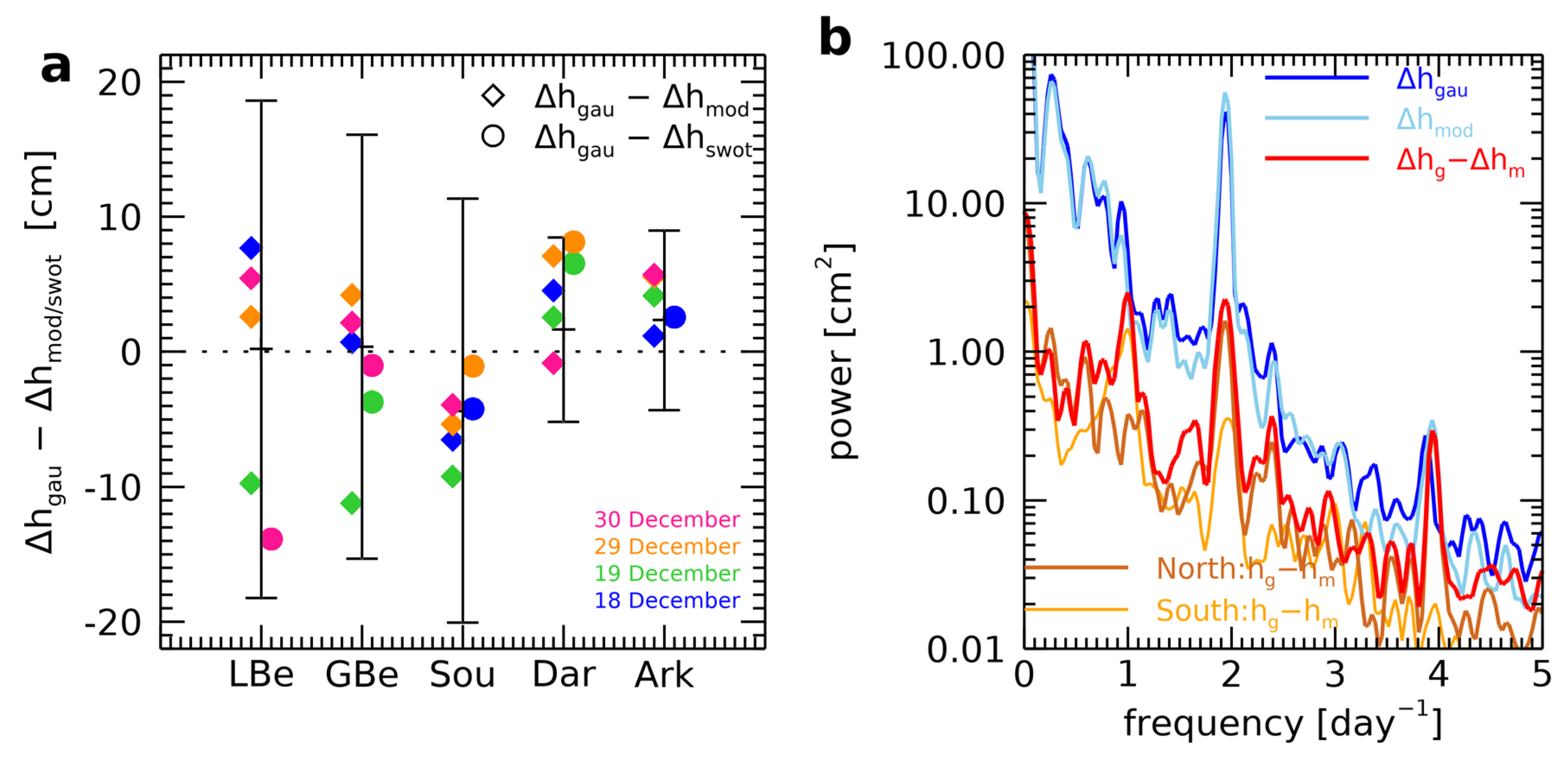
The mean and 2 σ range of the difference Δhgauge - Δhmodel is shown in Figure 7a for the Danish Straits, Darss Sill and Arkona Sea. The corresponding Δhgauge - Δhmodel and Δhgauge – Δhswot differences are indicated by diamonds and circles, respectively. The mean offset of Δhgauge - Δhmodel is close to zero for most straits. Exceptions are The Sound and the region across the Arkona Sea. A closer analysis shows that the model levels are by more than 5 cm higher than the gauge readings at Viken and Sassnitz and by almost 3 cm at Ystad. The reason for this could be either inconsistent vertical datums of these stations or deficiencies in the circulation simulated by BSH-HBMnoku. The corresponding differences between the model and SWOT are consistent for the Arkona Sea, but less consistent for The Sound. This might be an indication that the differences at The Sound are more model related and in the Arkona Sea rather related to the gauge datums. The Δhgauge - Δhswot differences are within the 2 σ range of the Δhgauge - Δhmodel differences and are close to each other in most cases. Exceptions are the Great Belt on 19 December and the Little Belt on 30 December. On 19 December, the sea level gradient along all Danish Straits seems to be overestimated by the model. On 30 December, the high levels recorded by SWOT in the northern part of the Little Belt are most probably not realistic.
There are not enough SWOT data available to study spectral differences between SWOT and tide gauge time series. However, many aspects related to systematic differences between coastal tide gauges and mean sea level over larger offshore areas should be similar for model and SWOT data. The power spectrum of the north-south height differences Δhgauge, Δhmodel and Δhgauge - Δhmodel is shown in Figure 7b. The model diverges from the tide gauges mainly on the half-daily and daily bands. Analysis of the height differences shows that the differences in the Kattegat (North) are mainly in the half-daily band, while the differences in the Western Baltic are mainly in the daily band. This suggests that the main differences between SLi from tide gauges and model are due to quarter and half daily ocean tides in the Kattegat area and are most likely related to Baltic seiches in the western Baltic area.
5. Conclusions
The recently launched SWOT mission provides a new set of spatial sea level observations for small-scale studies. During the course of the moderate MBI event in December 2023, there have been six SWOT overflights in the Kattegat - Western Baltic Sea area. Unfortunately, the KaRIn data are not available for two overflights and the maximum of the MBI event was not covered. Nevertheless, there are two snapshots showing the large-scale sea level gradients at the beginning of MBI event and two right at the end, which exhibit the sea level patterns related to the concurrent moderate MBI event in December 2023 with unprecedented detail.
In general, MBI events can only be monitored by sparsely distributed tide gauges and by salinity and ocean current measurement at a few moorings [5,7]. Large-scale altimetry has previously been used to study the occurrence of MBI events [37]. However, as far as we are aware, high-rate nadir altimetry has not yet been used for observing MBI events. With currently ten active nadir altimetry missions in orbit, the area is covered almost daily allowing to monitor the dominant flow processes in the area [38] and to provide additional information for spatial scales larger than 50 km. On 22 December, during maximum sea level gradients in the Danish Straits, Sentinel-6 MF observed a large-scale sea level difference of more than 130 cm between the western Kattegat and the western Arkona Sea, which is by almost 10% larger than simulated. However, not all missions provide stable and valid data in coastal regions, and the spatial resolution of the 1-D sea level measurements is not sufficient to resolve and understand the transient processes in this area [29,32]. The good agreement between the nadir and SWOT KaRIn altimetry provides confidence in the KaRIn data, especially considering that the observations may be separated by up to two days. Finally, tide gauge data can be used to detect unreliable SWOT KaRIn data.
SWOT KaRIn observations and the simulations with the regional 3-D BSH-HBMnoku ocean circulation model are in good agreement for most aspects. However, there are long wavelength differences that appear to be related to model deficiencies on daily to sub-daily time scales. In addition, the SWOT data have many fine scale structures like eddies and fronts that are not adequately modelled. Validation of these features is beyond the scope of this study, but the features appear to be plausible. This study shows that SWOT KaRIn altimetry provides valuable additional information about the transient processes in the region. Although the 2003 MBI event was only moderate, the underlying processes are the same as for very strong MBI events. The temporal sampling rate is not adequate for the process under consideration, but the SWOT observations together with high-rate nadir altimetry can significantly improve the existing in-situ monitoring.
Author Contributions
Conceptualization, S.E., H.D. and T.S.; methodology, S.E. and T.S.; software, S.E. and T.S.; data curation, S.E., T.S., R.S.; writing—original draft preparation, S.E.; writing—review and editing, S.E., T.S., H.D. and R.S.; visualization, S.E. All authors have read and agreed to the published version of the manuscript.
Funding
RS acknowledges funding by the TIDUS project withing the NEROGRAV research unit (DFG Research Unit 2736, Grant: TH864/15-2).
Data Availability Statement
The SWOT L2_LR_SSH data product is produced and made freely available by the joint SWOT (NASA/JPL and CNES) project. L2_LR_SSH product quality is not final and will be affected by some evolutions as the SWOT project team makes progress on science data processing algorithms and instrument calibrations. SWOT project, 2023. SWOT Level-2 KaRIn Low Rate SSH Expert (v2.0). CNES. https://doi.org/10.24400/527896/A01-2023.015. High-rate Level 2 nadir altimetry data from the Cryosat-2, Saral, Sentinel-3A, Sentinel-3B, Jason-3, Sentinel-6 MF, HY-2B, HY-2C, HY-2D and the SWOT mission are corrected and processed within GFZ’s ADS. The high-rate instantaneous sea level and sea level anomaly data from nadir altimetry processed by GFZ’s ADS and used for this study can be provided upon request by the authors. The Level 2 SGDR-F altimeter products of Saral, Jason-3 and SWOT nadir were produced and distributed by Aviso+ (https://www.aviso.altimetry.fr/), as part of the Ssalto ground processing segment. The paper contains modified Copernicus Sentinel data for Sentinel-3A and Sentinel-3B (https://dataspace.copernicus.eu/explore-data/data-collections/sentinel-data/sentinel-3), SRAL, Level 2 Marine, Non Time Critical (NTC), baseline 52, and for Sentinel-6 MF (https://user.eumetsat.int/data-access), Level 2, High Resolution (HR) Non Time Critical (NTC), baseline F08. European Space Agency provided Cryosat-2 L2 NOP-IOP-GOP SAR data, Version Baseline D. https://doi.org/10.5270/CR2-pbm8gdx. China ocean satellite were obtained from https://osdds.nsoas.org.cn. The authors would like to thank NSOAS for providing the HY-2 Level 2 SDR data free of charge. The tide gauge data were collated within the Copernicus Marine Service (In Situ) and EMODnet collaboration framework. Data is made freely available by the E.U. Copernicus Marine Service (CMEMS) and the programs that contribute to it. Baltic Sea - near real-time (NRT) in situ quality controlled observations, hourly updated and distributed by INSTAC within 24-48 hours from acquisition in average. https://doi.org/10.48670/moi-00032 (Accessed on 10-Feb-2025). The BSH-HBMnoku data “Modelled Forecast of Water Level Elevation (Coastal Grid) - series (publication: 2016-01-01, last change: 2024-02-14)” was made available from the Geman Bundesamt für Seeschifffahrt und Hydrographie (BSH) under Data License Germany, Version 2.0. https://www.geoseaportal.de/atomfeeds/z_file_fine_fc_en.xml (Accessed on 10-Feb-2025).
Acknowledgments
We thank Joachim Schwabe (BKG Leipzig/Germany) for most valuable help with tide gauge datum issues.
Conflicts of Interest
The authors declare no conflicts of interest. The funders had no role in the design of the study; in the collection, analyses, or interpretation of data; in the writing of the manuscript; or in the decision to publish the results.
Abbreviations
The following abbreviations are used in this manuscript:
| GDR | Geophysical Data Record |
| HBM | High-Resolution Model for the Baltic Sea - Baltic Operational Oceanography System |
| KaRIn | Ka-band Radar Interferometer |
| MBI | Major Baltic Inflow |
| SAR | Synthetic Aperture Radar |
| SLA | Sea Level Anomaly |
| SLi | Instantaneous Sea Level |
| SWOT | Surface Water and Ocean Topography Mission |
References
- Weisse, R.; Dailidiene, I.; Hünicke, B.; Kahma, K.; Madsen, K.; Omstedt, A.; Parnell, K.; Schöne, T.; Soomere, T.; Zhang, W.; et al. Sea Level Dynamics and Coastal Erosion in the Baltic Sea Region. Earth Syst. Dyn. Discuss. 2021, 1–40. [CrossRef]
- Lehmann, A.; Myrberg, K.; Post, P.; Chubarenko, I.; Dailidiene, I.; Hinrichsen, H.-H.; Hüssy, K.; Liblik, T.; Meier, H.E.M.; Lips, U.; et al. Salinity Dynamics of the Baltic Sea. Earth Syst. Dyn. 2022, 13, 373–392. [CrossRef]
- Lass, H.U.; Matthäus, W. On Temporal Wind Variations Forcing Salt Water Inflows into the Baltic Sea. Tellus Dyn. Meteorol. Oceanogr. 1996, 48. [CrossRef]
- Mohrholz, V.; Naumann, M.; Nausch, G.; Krüger, S.; Gräwe, U. Fresh Oxygen for the Baltic Sea — An Exceptional Saline Inflow after a Decade of Stagnation. J. Mar. Syst. 2015, 148, 152–166. [CrossRef]
- Mohrholz, V. Major Baltic Inflow Statistics – Revised. Front. Mar. Sci. 2018, 5, 384. [CrossRef]
- Stanev, E.V.; Peneva, E.; Chtirkova, B. Climate Change and Regional Ocean Water Mass Disappearance: Case of the Black Sea. J. Geophys. Res. Oceans 0. [CrossRef]
- Purkiani, K.; Jochumsen, K.; Fischer, J.-G. Observation of a Moderate Major Baltic Sea Inflow in December 2023. Sci. Rep. 2024, 14, 16577. [CrossRef]
- Stanev, E.V.; Pein, J.; Grashorn, S.; Zhang, Y.; Schrum, C. Dynamics of the Baltic Sea Straits via Numerical Simulation of Exchange Flows. Ocean Model. 2018, 131, 40–58. [CrossRef]
- Pham, N.T.; Staneva, J.; Bonaduce, A.; Stanev, E.V.; Grayek, S. Interannual Sea Level Variability in the North and Baltic Seas and Net Flux through the Danish Straits. Ocean Dyn. 2024, 74, 669–684. [CrossRef]
- Brüning, T.; Li, X.; Schwichtenberg, F.; Lorkowski, I. An Operational, Assimilative Model System for Hydrodynamic and Biogeochemical Applications for German Coastal Waters. Hydrogr. Nachrichten 2021, 6–15. [CrossRef]
- Abdalla, S.; Abdeh Kolahchi, A.; Adusumilli, S.; Aich Bhowmick, S.; Alou-Font, E.; Amarouche, L.; Andersen, O.B.; Antich, H.; Aouf, L.; Arbic, B.; et al. Altimetry for the Future: Building on 25 Years of Progress. Adv. Space Res. 2021. [CrossRef]
- Cipollini, P.; Calafat, F.M.; Jevrejeva, S.; Melet, A.; Prandi, P. Monitoring Sea Level in the Coastal Zone with Satellite Altimetry and Tide Gauges. Surv. Geophys. 2017, 38, 33–57. [CrossRef]
- Vignudelli, S.; Birol, F.; Benveniste, J.; Fu, L.-L.; Picot, N.; Raynal, M.; Roinard, H. Satellite Altimetry Measurements of Sea Level in the Coastal Zone. Surv. Geophys. 2019, 40, 1319–1349. [CrossRef]
- Esselborn, S.; Schöne, T.; Illigner, J.; Weiß, R.; Artz, T.; Huang, X. Validation of Recent Altimeter Missions at Non-Dedicated Tide Gauge Stations in the Southeastern North Sea. Remote Sens. 2022, 14, 236. [CrossRef]
- Pujol, M.-I.; Dupuy, S.; Vergara, O.; Sánchez Román, A.; Faugère, Y.; Prandi, P.; Dabat, M.-L.; Dagneaux, Q.; Lievin, M.; Cadier, E.; et al. Refining the Resolution of DUACS Along-Track Level-3 Sea Level Altimetry Products. Remote Sens. 2023, 15, 793. [CrossRef]
- Metzner, M.; Gade, M.; Hennings, I.; Rabinovich, A.B. The Observation of Seiches in the Baltic Sea Using a Multi Data Set of Water Levels. J. Mar. Syst. 2000, 24, 67–84. [CrossRef]
- Liebsch, G.; Novotny, K.; Dietrich, R.; Shum, C.K. Comparison of Multimission Altimetric Sea-Surface Heights with Tide Gauge Observations in the Southern Baltic Sea. Mar. Geod. 2002, 25, 213–234. [CrossRef]
- Madsen, K.S.; Høyer, J.L.; Tscherning, C.C. Near-Coastal Satellite Altimetry: Sea Surface Height Variability in the North Sea–Baltic Sea Area. Geophys. Res. Lett. 2007, 34, n/a-n/a. [CrossRef]
- Madsen, K.S.; Høyer, J.L.; Suursaar, Ü.; She, J.; Knudsen, P. Sea Level Trends and Variability of the Baltic Sea From 2D Statistical Reconstruction and Altimetry. Front. Earth Sci. 2019, 7. [CrossRef]
- Passaro, M.; Müller, F.L.; Oelsmann, J.; Rautiainen, L.; Dettmering, D.; Hart-Davis, M.G.; Abulaitijiang, A.; Andersen, O.B.; Høyer, J.L.; Madsen, K.S.; et al. Absolute Baltic Sea Level Trends in the Satellite Altimetry Era: A Revisit. Front. Mar. Sci. 2021, 8. [CrossRef]
- Elken, J.; Barzandeh, A.; Maljutenko, I.; Rikka, S. Reconstruction of Baltic Gridded Sea Levels from Tide Gauge and Altimetry Observations Using Spatiotemporal Statistics from Reanalysis. Remote Sens. 2024, 16, 2702. [CrossRef]
- Fu, L.-L.; Pavelsky, T.; Cretaux, J.-F.; Morrow, R.; Farrar, J.T.; Vaze, P.; Sengenes, P.; Vinogradova-Shiffer, N.; Sylvestre-Baron, A.; Picot, N.; et al. The Surface Water and Ocean Topography Mission: A Breakthrough in Radar Remote Sensing of the Ocean and Land Surface Water. Geophys. Res. Lett. 2024, 51, e2023GL107652. [CrossRef]
- SWOT Project, SWOT Level-2 KaRIn Low Rate SSH Expert (v2.0), 2024. [CrossRef]
- Schöne, T.; Esselborn, S.; Rudenko, S.; Raimondo, J.-C. Radar Altimetry Derived Sea Level Anomalies – The Benefit of New Orbits and Harmonization. In System Earth via Geodetic-Geophysical Space Techniques; Flechtner, F.M., Gruber, T., Güntner, A., Mandea, M., Rothacher, M., Schöne, T., Wickert, J., Eds.; Springer Berlin Heidelberg: Berlin, Heidelberg, 2010; pp. 317–324 ISBN 978-3-642-10227-1.
- Dach, R.; Schaer, S.; Arnold, D.; Kalarus, M.S.; Prange, L.; Stebler, P.; Villiger, A.; Jäggi, A. CODE Final Product Series for the IGS, Astron. Inst. Univ. Bern 2020. https://boris.unibe.ch/197025/.
- Petit, G.; Luzum, B. IERS Conventions (2010); IERS Technical Note; Verlag des Bundesamts für Kartographie und Geodäsie: Frankfurt am Main, 2010; ISBN 3-89888-989-6.
- Desai, S.; Wahr, J.; Beckley, B. Revisiting the Pole Tide for and from Satellite Altimetry. J. Geod. 2015, 89, 1233–1243. [CrossRef]
- Lyard, F.H.; Allain, D.J.; Cancet, M.; Carrère, L.; Picot, N. FES2014 Global Ocean Tide Atlas: Design and Performance. Ocean Sci. 2021, 17, 615–649. [CrossRef]
- Schaeffer, P.; Pujol, M.-I.; Veillard, P.; Faugere, Y.; Dagneaux, Q.; Dibarboure, G.; Picot, N. The CNES CLS 2022 Mean Sea Surface: Short Wavelength Improvements from CryoSat-2 and SARAL/AltiKa High-Sampled Altimeter Data. Remote Sens. 2023, 15, 2910. [CrossRef]
- Jousset, S.; Mulet, S.; Greiner, E.; Wilkin, J.; Vidar, L.; Dibarboure, G.; Picot, N. New Global Mean Dynamic Topography CNES-CLS-22 Combining Drifters, Hydrological Profiles and High Frequency Radar Data. ESS Open Archive, Dec. 2023. [CrossRef]
- Carrère, L.; Lyard, F. Modeling the Barotropic Response of the Global Ocean to Atmospheric Wind and Pressure Forcing - Comparisons with Observations. Geophys. Res. Lett. 2003, 30. [CrossRef]
- Omstedt, A.; Elken, J.; Lehmann, A.; Leppäranta, M.; Meier, H.E.M.; Myrberg, K.; Rutgersson, A. Progress in Physical Oceanography of the Baltic Sea during the 2003–2014 Period. Prog. Oceanogr. 2014, 128, 139–171. [CrossRef]
- Le Traon, P.; Ali, A.; Fanjul, A.; Behrens, A.; Stanev, E.; Staneva, J., The Copernicus Marine Environmental Monitoring Service: Main Scientific Achievements and Future Prospects, Special Issue Mercator Océan Journal; 2017. [CrossRef]
- Schwabe, J.; Ågren, J.; Liebsch, G.; Westfeld, P.; Hammarklint, T.; Mononen, J.; Andersen, O.B. The Baltic Sea Chart Datum 2000 (BSCD2000): Implementation of a Common Reference Level in the Baltic Sea. Int. Hydrogr. Rev. 2020, 63–82. https://journals.lib.unb.ca/index.php/ihr/article/view/33085.
- Lorenz, M.; Viigand, K.; Gräwe, U. Untangling the Waves: Decomposing Extreme Sea Levels in a Non-Tidal Basin, the Baltic Sea. Nat. Hazards Earth Syst. Sci. Discuss. 2024, 1–28. [CrossRef]
- Jönsson, B.; Döös, K.; Nycander, J.; Lundberg, P. Standing Waves in the Gulf of Finland and Their Relationship to the Basin-Wide Baltic Seiches. J. Geophys. Res. Oceans 2008, 113. [CrossRef]
- Stramska, M.; Aniskiewicz, P. Satellite Remote Sensing Signatures of the Major Baltic Inflows. Remote Sens. 2019, 11, 954. [CrossRef]
- Elyouncha, A.; Broström, G.; Johnsen, H. Synergistic Utilization of Spaceborne SAR Observations for Monitoring the Baltic Sea Flow Through the Danish Straits. Earth Space Sci. 2024, 11, e2024EA003794. [CrossRef]
Figure 1.
Map showing the geographical terms used in this paper. The Danish Straits include: Little Belt, Great Belt and The Sound. Tide gauges in the Danish Straits are shown in orange, those in the Western Baltic in yellow.
Figure 1.
Map showing the geographical terms used in this paper. The Danish Straits include: Little Belt, Great Belt and The Sound. Tide gauges in the Danish Straits are shown in orange, those in the Western Baltic in yellow.
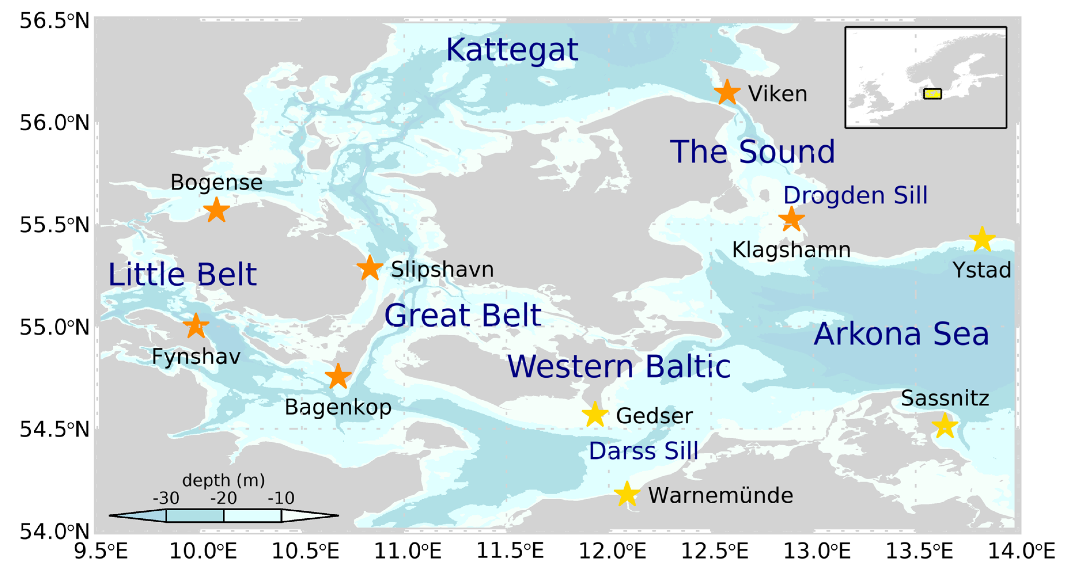
Figure 2.
Sea level difference (Δh) based on tide gauges, (a) hNorth-hSouth along the Danish Straits, where positive values imply transport to the south. (b) hSouth-hNorth across the Western Baltic near Darss Sill and across the Arkona Sea, where positive differences imply barotropic transport to the East. The time series are 3 h boxcar filtered. SWOT overflights are indicated by light gray vertical lines, the Sentinel-6 MF overflight is indicated by a gray vertical line, periods where nadir altimetry is compared with SWOT overflights are shaded gray.
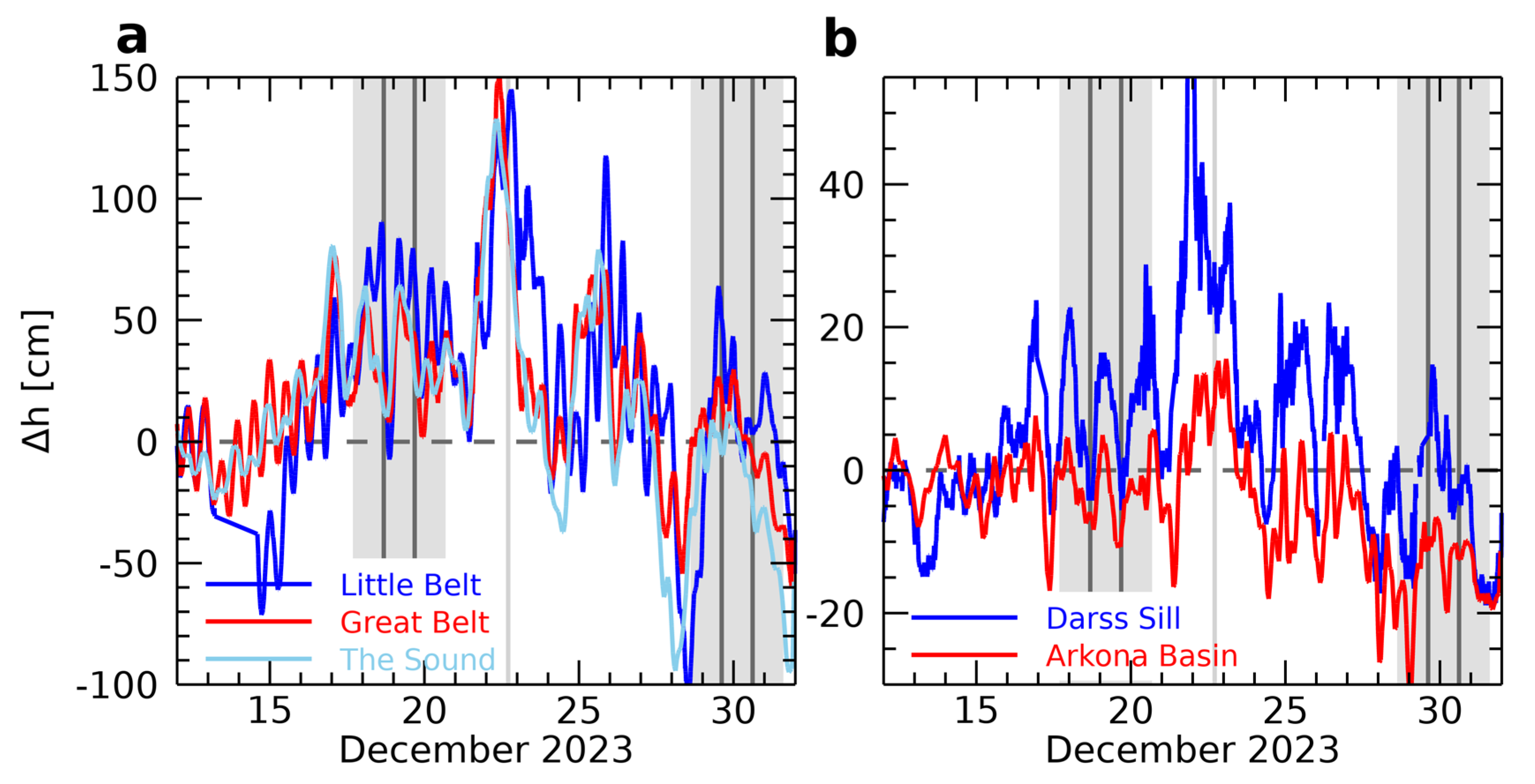
Figure 3.
(a) Instantaneous sea level (SLi) on 22 December 17:05 UTC observed by Sentinel-6 MF and simulated by BSH-HBMnoku based on tide gauges. (b) Sea level differences between nadir altimetry and model.
Figure 3.
(a) Instantaneous sea level (SLi) on 22 December 17:05 UTC observed by Sentinel-6 MF and simulated by BSH-HBMnoku based on tide gauges. (b) Sea level differences between nadir altimetry and model.
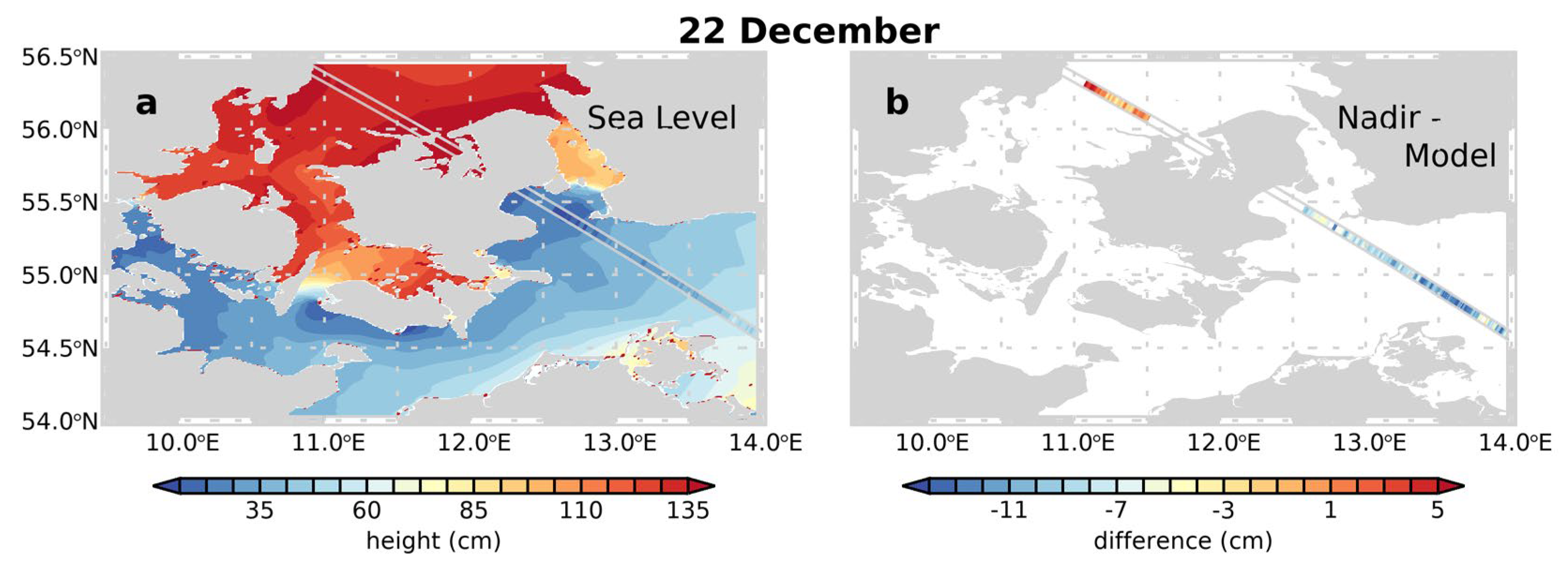
Figure 4.
Instantaneous sea level (a, d) from SWOT (KaRIn and nadir) measurements, (b, e) from the BSH-HBMnoku model and (c, f) difference SWOT minus BSH-HBMnoku (a, b, c) on 18 December 2023 16:26 UTC (d, e, f) and 19 December 2023 16:27 UTC.
Figure 4.
Instantaneous sea level (a, d) from SWOT (KaRIn and nadir) measurements, (b, e) from the BSH-HBMnoku model and (c, f) difference SWOT minus BSH-HBMnoku (a, b, c) on 18 December 2023 16:26 UTC (d, e, f) and 19 December 2023 16:27 UTC.
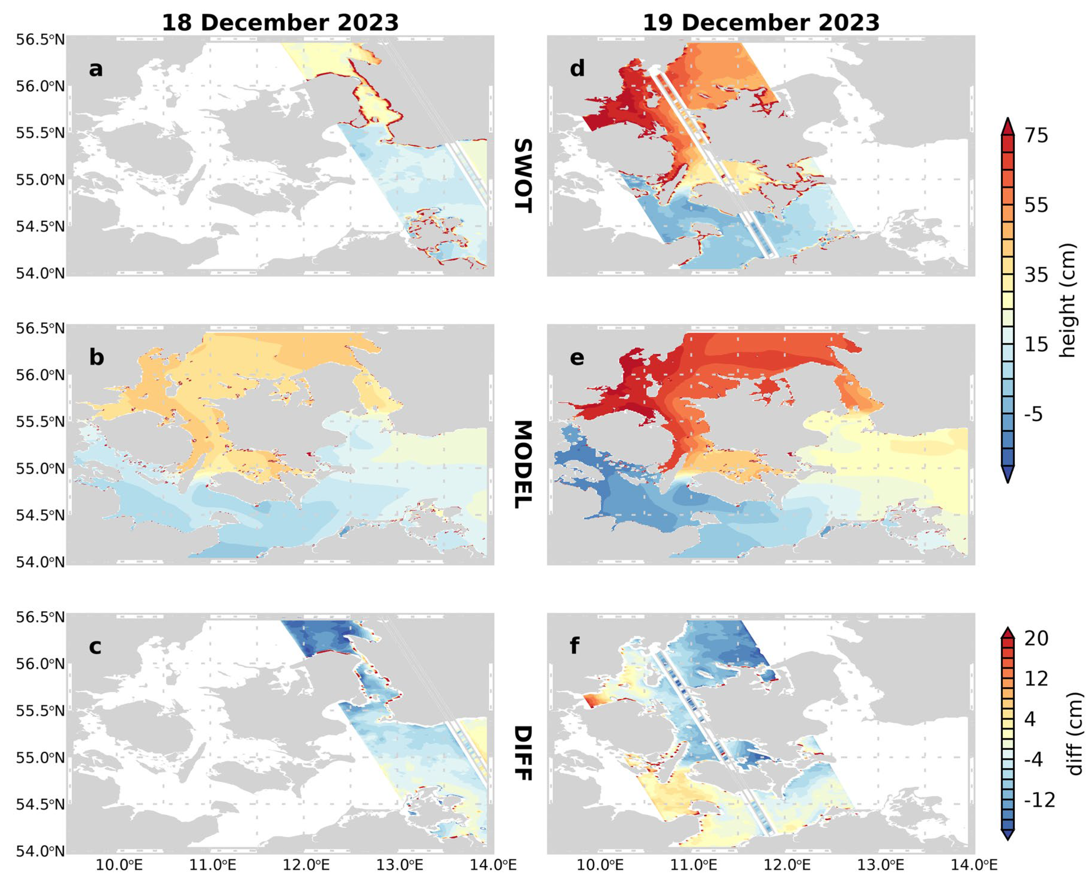
Figure 5.
Instantaneous sea level (a, d) from SWOT (KaRIn and nadir) measurements, (b, e) from the BSH-HBMnoku model and (c, f) difference SWOT minus BSH-HBMnoku (a, b, c) on 29 December 2023 14:49 UTC (d, e, f) and 30 December 2023 14:50 UTC.
Figure 5.
Instantaneous sea level (a, d) from SWOT (KaRIn and nadir) measurements, (b, e) from the BSH-HBMnoku model and (c, f) difference SWOT minus BSH-HBMnoku (a, b, c) on 29 December 2023 14:49 UTC (d, e, f) and 30 December 2023 14:50 UTC.
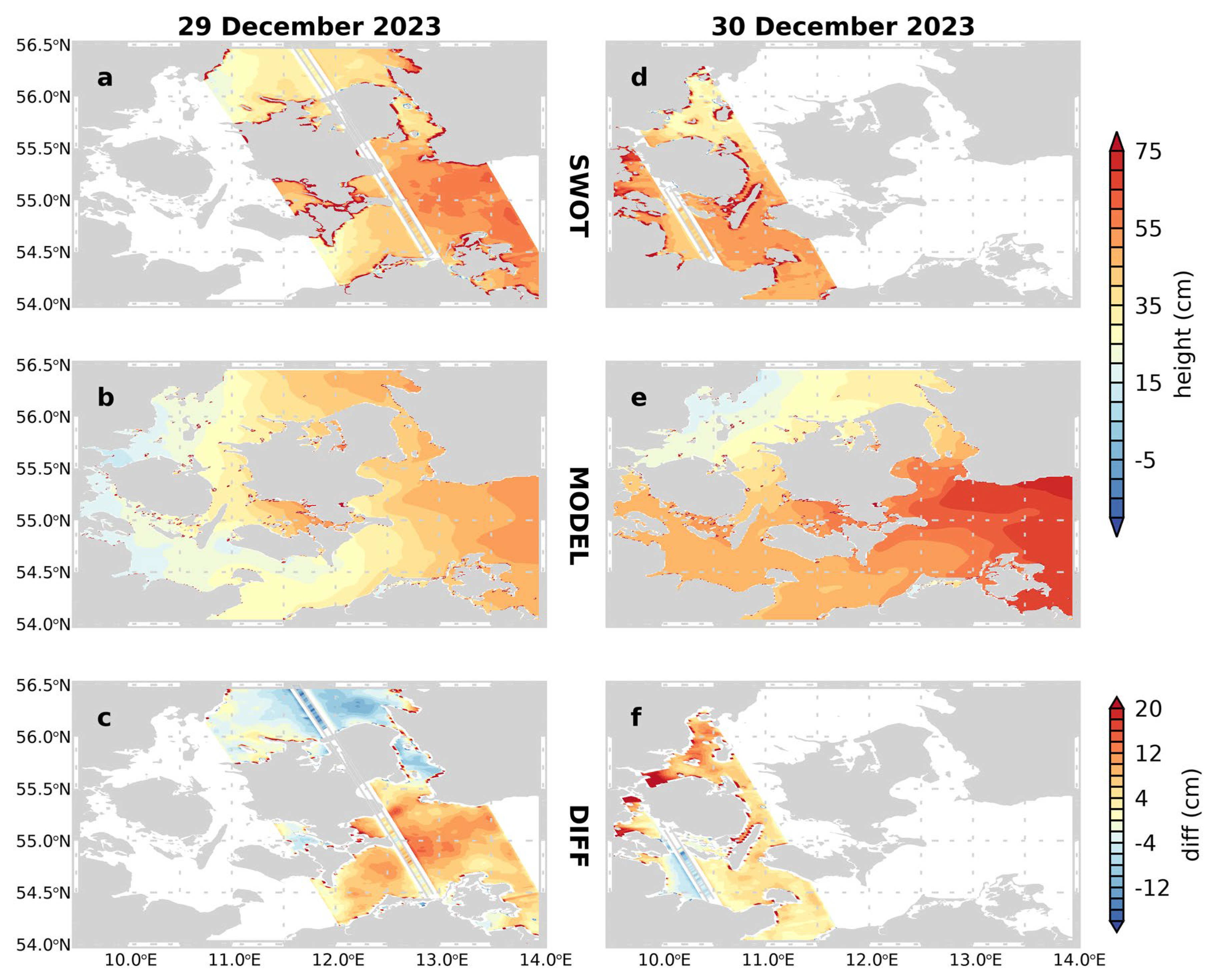
Figure 6.
(a,b) Sea level anomalies (SLA) from SWOT KaRIn and all available nadir altimetry for two 3-day periods (a) inflow (17-20 December 2023 16:30 UTC) and (b) post-inflow (28 -31 December 2023 14:50 UTC). (c, d) Difference of instantaneous sea level (SLi) from altimetry (all nadir and SWOT KaRIn) vs. BSH-HBMnoku model for (c) inflow and (d) post-inflow. Tide gauge locations are indicated by green stars.
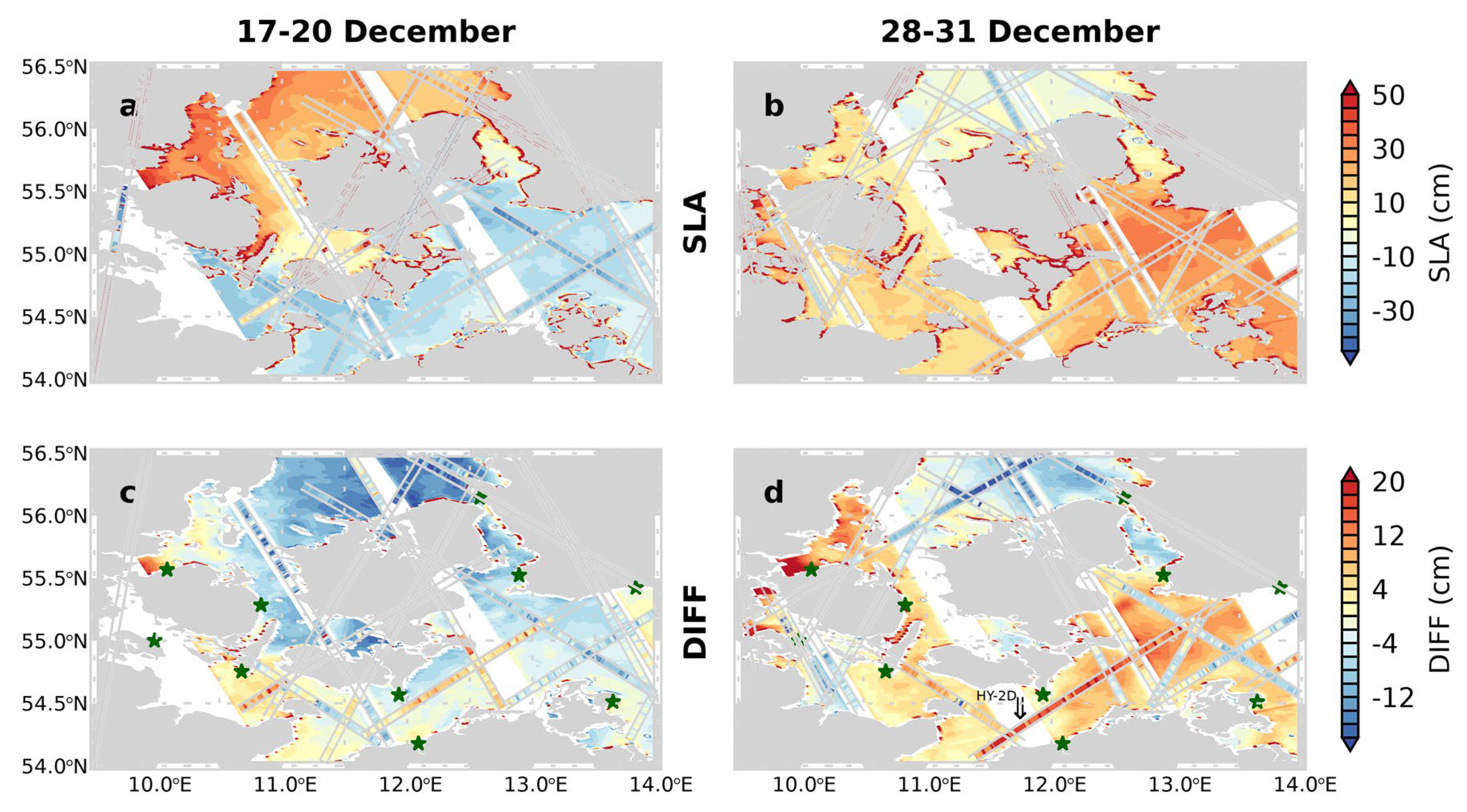
Figure 7.
Comparison of north-south height difference (Δh) from gauge, model and SWOT. (a) Mean and 2 σ range of Δhgauge-Δhmodel in December 2003 for Little Belt (LBe), Great Belt (GBe), The Sound (Sou), Darss Sill (Dar) and Arkona Sea (Ark). Symbols show the values during SWOT overflights, diamonds for Δhgauge-Δhmodel, circles for Δhgauge-Δhswot. Overflights are colour coded. (b) Power spectra averaged over the three Danish Straits. Spectra of Δh from gauges (blue), model (light blue) and of Δhgauge-Δhmodel (red), and of SWOT/model height difference in the Kattegat (brown) and in the Western Baltic (orange).
Disclaimer/Publisher’s Note: The statements, opinions and data contained in all publications are solely those of the individual author(s) and contributor(s) and not of MDPI and/or the editor(s). MDPI and/or the editor(s) disclaim responsibility for any injury to people or property resulting from any ideas, methods, instructions or products referred to in the content. |
© 2025 by the authors. Licensee MDPI, Basel, Switzerland. This article is an open access article distributed under the terms and conditions of the Creative Commons Attribution (CC BY) license (http://creativecommons.org/licenses/by/4.0/).
Copyright: This open access article is published under a Creative Commons CC BY 4.0 license, which permit the free download, distribution, and reuse, provided that the author and preprint are cited in any reuse.


