
Submitted:
11 February 2025
Posted:
12 February 2025
You are already at the latest version
Abstract
The determination of the friction coefficients for uniform flows over very rough bottoms is a long-standing problem in open channel hydraulics and river engineering. This experimental study reports the surface deformation, Darcy and Manning’s friction coefficients obtained from measurements on steady, turbulent (6,058≤Re≤28,502) and subcritical flows (0.14≤Fr≤0.52) over large roughness elements, where Fr,Re is the flow’s Froude and Reynolds number. The experiments were carried out in a rectangular inclined flume with a train of half-cylinders at the bottom, whose radius fall into the range 20 mm≤a≤50 mm. These obstacles are such that 1.45≤hN/a≤4.41 and e/a=12.8 far all the experimental runs, with hN the normal flow depth and e the spacing between the cylinders. The relative amplitude (Δh/a) of the surface profiles was analyzed showing a close correlation with hN/a, Re and Fr. Our results lead to very high values of the Darcy friction factor f following scaling laws of the type f∝(hN/a)n^ with n^<0 independent on a, and f∝Reβ, where β<0 closely related to a. Scaling laws for the Manning roughness coefficient (n) were also studied and reported.
Keywords:
turbulent flow
; macroroughness
; rough flows
; friction factor
; Manning friction coefficient
1. Introduction
Free surface flows over rough and very rough bottoms are ubiquitous in nature and industry. Environmental river floods, fluvial streams over sedimentary bedforms, or over large particles such as boulders and rocks usually fall into this scenario [1,2,3,4]. However, this situation can also be found in the mining industry with sedimentary bedforms created by solid-liquid suspensions flows [5], or the atmospheric boundary layer dynamics around urban buildings [6]. For the first scenario, many studies have attempted to characterize the friction properties from numerical and experimental point of views [2,3,7,8,9,10,11,12,13,14,15,16,17,18,19,20]. Most of these studies have recognized the influence of many hydraulic parameters, such as the flow rate (Q), the average velocity (V), the flow depth (h), and the bottom slope (i), to name a few. However, despite of the progress reached with the previous studies, a proper comprehension about the role played by the roughness size and their spatial distribution on the flow dynamics, remains elusive and poorly studied in current literature on the topic.
To this concern, Bazin and Darcy [21] pioneered this topic conducting experiments in a large sloped flume in Bourgogne (France), sticking regularly spaced square ribs of height k at the bottom. These experiments are currently known as k-type rough flows [22]. Bazin recognized that the Chezy law can also be applied to describe open-channel flows, which currently takes the Darcy-Weisbach form [23,24]. For open-channel flow this law can be written as follows:
where i is the flume bottom slope, V the cross-sectional average velocity, R is the hydraulic radius of the uniform flow and f, the Darcy friction factor. According to Lim [24], Bazin suggested that this factor is primarily related to the relative roughness ratio and not necessarily, the bottom slope. In addition, Bazin proposed an empirical relation for the resistance coefficient valid in the range , where is the Reynolds number. Bazin’s experimental data was so extensive, as impressive, and later used to determine the roughness coefficient involved in the Manning law [24].
According to Davis [25], Morris [26,27] suggested that the longitudinal spacing e between roughness elements in the flow direction, is one of the key parameters when analyzing the nature of these flows. To this concern, Chow [23] described three possible roughness regimes depending on the magnitude of e: (1) an isolated-roughness flow, when roughness elements are so far apart that the wakes generating just downstream each element are completely developed and dissipated before reaching the next element; (2) a wake-interference flow, when these elements are placed so that wakes at each element interfere with those developed at the next one and (3), a quasi-smooth flow, where these elements are so close together that the flow skims the crests of roughness, but the grooves between them form dead zones where stable eddies can be observed. A key observation from these experiments is that cases (1) and (2) are the regimes influencing the most the flow friction, as well as the deformation of the free surface [23]. From the properties analysis of the urban atmospheric boundary layer, Oke [6,28] proposed that the regime (1) occurs when , the case (2) when , and (3) when .
Morris [26] also pointed about the key role played by the submergence ratio , i.e the ratio of normal depth to roughness height, when studying the presence of wake-interference flow commonly observed in shallow flows. Morris also proposed a critical spacing value () to fix the limit between the isolated roughness and the wake interference flow, at high Reynolds number. Nikora et al. [29,30] confirmed Morris’ observations from the analysis of fluvial streams over gravel-boulder beds. Nikora identified four hydrodynamics layers influenced by the bottom roughness and the ratio . These regimes are influenced not only by the local geometry of roughness, but also the spatial distribution of these elements.
Therefore, if the distribution of roughness elements affects the flow structure around them, an influence on the overall friction properties of the flow should be observed, particularly in the magnitude and properties of the Darcy friction coefficient f. In this context, Bathurst [2] concluded that most of resistance equations were subject to large errors for shallow water flows where the free surface is prone to deform by the influence of large roughness elements, opening a connection between surface deformation and flow friction. Lawrence studied this connection by analyzing the hydraulics of overland flow on rough granular surfaces [31], but also from experiments of steady, uniform flows over rough beds formed by isolated half-spheres [32]. Particularly, this author recognized a close relationship between f and identifying three regimes [32], that is, (i) partial inundation regime (), (ii) marginal inundation () and (iii), well-inundated regime (). In these last two regimes the Darcy friction factor can be roughly represented by the following laws:
where , and . The structure of Eq.3 is similar to Nikuradse log-law reported for rough flows [33], also found by Bayazit [34] studying the resistance laws of large-scale roughness flow. Lawrence also measured the surface waves induced by the protrusions finding an additional flow resistance induced by such elements, named by tha author as wave resistance. Lawrence’s results confirm that Bazin’s prediction about the role played by the relative roughness () was correct. McSherry et al. [35] studied the transitional effect for k-type rough flows performing large-eddy simulations and experiments on a flume. This author found that the logarithmic layer predicted by Nikora et al. [29,30] vanishes for low submergence ratios (), but it may appear for higher ratios (). McSherry observed weak and undular jumps at the free surface, which seem to affect the overall momentum balance and drag.
Although the cited studies have helped to progress on the topic, little attention has been paid to the geometry effects of the asperities [36]. Forbes [37] for example analyzed the flow around a single half-cylinder located at the bottom of a flume showing that the flow surface can be recovered by using the potential flow equations. Vigie [38] experimentally studied this interaction using a similar configuration, reporting different downstream surface deformation patterns and proposing a topological classification for such patterns. Vigie identified a key role of the Froude number in this dynamics, and the parameter on such classification, with h the approximation water depth and a measure of the bottom roughness (a is the cylinder radius).
Ryu et al. [39] is one of the few studies performing measurements about the friction factor for two-dimensional flows over a train of ribs of uniform height, but different shapes (e.g. semi-circles, triangles, squares, and dunes). Ryu et al. found that f is strongly influenced by the shape of the ribs, increasing up to in the range , but decreasing notoriously to values slightly below the value when (with e measured between the centers of the obstacles). In the light of the above, in this research the structure of the classical resistance laws observed on steady, uniform, subcritical turbulent flows over a bed formed by large half-cylindrical ribs, was experimentally studied. Particularly, the role played by the spacing e between the cylinders and the size of them, is emphasized exploring the scaling laws arising from this analysis and its impacts the connection with the hydrodynamical flow conditions.
2. Experimental Set-Up
2.1. Materials
The experiments were carried out at the recirculating flume of the Laboratory of the School of Civil Engineering of the Pontificia Universidad Católica de Valparaiso, Chile. The lenght of the flume is 9.90m, a rectangular cross-section of width 0.358 m, and a total height 0.40 m. The bottom slope reaches values up to 1.50%. A centrifugal pump feeds the system, with a variable frequency drive (VFD) controlling the flow rate (Q) into the range 3 to 15 Ls−1. The obstacles are half-cylinders made of high-density styrofoam, of radius 20, 25, 35 and 50 mm. A sketch of the experimental set-up is depicted in Figure 1. All the obstacles were covered with a thin layer of waterproof paint to reduce the surface asperities, facilitating the hydrodynamical interaction with the stream. The flow depth measurements were conducted with three ultrasonic probes MICROSONIC Co. model PICO 100, operating simultaneously and located above the surface at any time and fixed frequency rate 200 kHz. The precision of the probes is around 1% of measures. The Plexiglas sidewalls of the flume allows for the flow visualization along the channel. Films and images of the free surface were recorded from one side using a Canon EOS Rebel T6/60fps camera.
2.2. Methodology
For a given experiment, N cylinders of diameter D locate at the bottom of the flume, separated a distance e, measured center to center between the obstacles. As many arrays, as diameters of obstacles were tested in the campaign (cf. Table 1). These arrays are such that the aspect ratio holds for all the experiments. According to Chow [23] and Oke [6] this choice lead us to the isolated-roughness regime, that is, the scenario influencing the most the flow friction. A central region of the flume of length m was fixed to carry out all the flow depth measurements.The bottom slope was fixed for all the purposes, as well. In this scenario the flow far from the entrance becomes uniform and independent of the entry and exit effects. Water ascends trough a tranquilization chamber reducing turbulence entrance effects. The flow freely enters the channel discharging to a tank from where is reconducted to the recicurlating pipeline as shown in Figure 1.
The first cylinder of the array () is located at the entry section of the flume and the last one (), 1 cm before reaching the discharge section. According to Monin and Yaglom [40], the distance required for the boundary layer to cover the flow depth can be evaluated from the law:
where is the boundary layer thickness, is the distance from the leading edge of the flume, is the friction velocity and U the approximation velocity. By considering , the required distance can be readily evaluated by imposing , obtaining for to fall in the range 0.41 m 1.91 m. Notice that Pokrajac et al. [41] reported close values for in a similar flume, so the flow can be considered uniform in the analysis region. Once the flow rate is fixed the steady regime is quickly reached in the flume. In this scenario, flow depth measurements were conducted at different stations along the center, left and right axes of the flume. The stations number M depends on the size of cylinders, that is, 53 for mm to for mm. Measurements on the right and left axes were made at not less than 1 cm from the walls, reducing boundary effects on probe measurements. The instantaneous flow depth is easily obtained from the relation:
where is the real height measured by each probe and , with a bottom vertical coordinate ( for a flat surface and when the measuring station is just above a cylinder). The flow depth was measured for around s at each position. This period was large enough to ensure the convergence of measures. The laboratory temperature was regularly controlled to reduce environmental effects on the probe’s operation. Using an Arduino-based electronic system, the signal emitted by each probe was communicated and registered to a PC. The time average of the flow depth was estimated as:
where R is the total number of time measures at each station ( 2,024).
2.3. Estimation of the Normal Depth, the Froude and Reynolds Number
From the Eq.6 the spatial average of the flow depth in the region of interest can be estimated as follows:
where M is the number of stations along the flume (∼53 to 87 points). The streamise average hydraulic radius R and mean velocity of the flow V can be calculated from Eq.7 as follows:
The overall Froude and Reynolds numbers, two characteristic dimensionless parameters for free surface flows, were determined as:
where is the fluid kinematic viscosity (m2s−1). Hereinafter, the Equation 7 is considered a reasonable estimator for the normal depth of the uniform flow in the analysis region in every experiment. Data standard errors are usually not larger than ±1.5 mm for this last quantity. The minimum flow rate (3.0 ) assures the full immersion of the cylinders, that is, 1.48 for all the experiments. The normal depth with no obstacles in the flume, denoted as , was measured for the same experimental conditions falling into the range 15.8 mm42.7 mm. Accordingly to Chow [23], the turbulent regime in open channel flows occurs when , where 1,000 is considered a critical value for laminar-turbulent flow transition. Finally, the overall Froude number falls in the range 0.140.52, whereas 6,05828,502 conducting to subcritical flows in turbulent regime.
3. Results & Discussion
3.1. Deformation of the Free Surface and Backwater Profiles
Figure 3, Figure 4 and Figure 5 show the flow characteristics over the train of half-cylinders for different hydraulic conditions. Figure 3 shows the shape of the free surface for obstacles of radius 25 mm, and increasing flow rates. If in this case the free surface is regular with well-defined and static peaks and valleys at low flow rates (Figure 3a), when the flow rate increases the surface quickly becomes irregular, whose peaks and valleys can change their positions over time as seen later (Figure 3c). The amplitude () of these peaks become very important particularly for high flow rates. The deformation patterns observed in Figure 3a,b were the most common observed in our experimental campaign, even for different cylinder sizes and flow rates.
Figure 4 shows instead the evolution of the surface deformation patterns for increasing sizes of the cylinders, and fixed flow rate (). A counterintuitive observation is that these deformations are not necessarily larger for larger obstacles, as might be expected. On the other hand, the surface between obstacles quickly recovers when the size of the obstacles, and therefore the distance between them, increases. Another interesting element is that only one valley occurs between two consecutive obstacles, taht is located closer to the first element. As the size of the obstacles increases, particularly into the range 35 mm, the surface profile appear much more stable over time, forming a train of bumps, similar to undular jumps, whose position is almost-constant in time.
Such an invariance in these deformation patterns becomes less clear when dealing with smaller obstacles at high flow rates. Figure 5 shows the evolution of the surface over time periods of around 1 s, for cylinders of radius 25 mm. The peaks move in the upstream direction, and their amplitude decreases in these cycles (see the red arrows). Although the physical or statistical properties of were not studied, we believe that the structure of this parameter should depends on the flow rate. This variability and the instability of the surface was frequently observed for small cylinders (20, 25 mm). This last observation emphasizes the difficulty of studying the structure of surface waves, whose stationary behavior seems to be restricted to very specific conditions of the obstacles and the turbulent intensity.
Based on the ultrasound probe measurements, the shape of the backwater profiles was obtained and plotted for all the experimental runs. Figure 6 show these profiles for all the arrays and increasing flow rates. The normal depth was indicated in Figure 6a, calculated from Eq.7. As mentioned, all these profiles show a bumping behavior whose peaks/valleys are uniformly distributed along the analysis window. These bumps are not, nevertheless, exactly symmetrical and their amplitude peaks do not occur just over each cylinder, but just in a downstream position close to it. This pattern was reported by Vigie [38], who carried out experiments with a single cylinder interacting with a subcritical flow in an inclined flume. Lawrence [32] also reports similar features obtained from experiments of turbulent flow over a bed of spheres. Lawrence named this pattern as undular jumps.
The amplitude of deformations was calculated as the streamwise average of the difference between the peaks and valleys of each hydraulic profile (cf. Figure 6a). Figure 7 shows that although the relative amplitude, is closely correlated with the parameters , and , no clear empirical function reasonably fits these datasets. The only clear observation is that while these parameters increase, so does , but not necessarily by itself, reaffirming the need of using relative scales for analyzing this phenomenon.
3.2. Distribution of the Normal Depth
The inset of Figure 8a compares the normal depth measured over the cylinders (), and the same depth measured without them (). The datasets organize around straight lines, whose slopes depend on the radius a. The main plot of Figure 8a aims to generalize this result, comparing the relative normal depth to , where h can be the critical depth , or . These curves can be represented by the following function:
where s is the slope of each line, where when , but when . The critical depth was calculated as , where is the flow rate per unit width. As expected, Eq.11 shows that , and , meaning that the normal depth always turns out to be greater than the depths measured with no obstacles on the flume emphasizing the significant effect induced by the cylinders on the stream behavior.
The inset of Figure 8b plots the normal height and the Froude number for all the experimental runs. Once again, datasets organizes around shifted straight lines of slope and intercept . The distribution of these two fitting parameters can be observed in Figure 8c,d. These plots summarizes in the relation , where is closely related to the radius of the obstacles. Notice that the distribution of is not strictly linear, but presents decreasing values for larger obstacles. This is coincident with the qualitative observations introduced in Figure 3 and Figure 4. Some physical attenuation mechanisms are maybe involved in the growing process of the surface waves when the flow interacts with the big cylinders.
If we divide the normal depth by the size scale a and we compare it to the overall Froude number we obtain the plot of Figure 9a. The observed curve can be described by the next function:
where and are fitting parameters. The non-linearity observed in the curve () is the result of the non-linearity of coefficients . Figure 9b shows, instead, the relative height compared to Reynolds number expressed in the form , where (see Section 6). Four straight lines of parameters arises, each of them related to a. These curves can also be described by the following relation:
Accordingly to Figure 9c,d, the fitting parameters can be described by the next functions:
where and . The coefficient 20 mm is just the size of the smaller cylinder and is taken in this study just as a reference value, arbitrarily chosen, to build dimensionless plots.
3.3. About the Darcy Friction Coefficient
Figure 10a compares the Darcy-Weisbach friction coefficient (Eq.1), expressed in the form , to the submergence ratio for all the experimental runs. Data organizes reasonably well around a single curve described by the following general function:
where and . Although the structure of Eq.15 is similar to the curve proposed in [32,34], our measurements strictly fall between the two hydraulic regimes proposed by Lawrence. The marginal inundation curve () introduced in Section 1 falls below our data, whereas the well-inundated regime () overestimates our measurements. Just for comparison purposes, the friction factor was also computed from the classical Colebrook-White expression (). This last formula was adapted for open-channel flow conditions, valid into the range [23]:
where R is the hydraulic radius and the mean size of roughness’ bottom. The Eq.16 was numerically solved using conventional methods, considering as a rough measure of these asperities. Figure 10a shows the solution of Eq.16 through the curve versus , for all the experiments. Once again, the Colebrook-White equation overestimates our data, together with the results of [32]. The inset of Figure 10a compares f and the relative depth using the same dataset. This curve leads to an alternative expression for the Darcy factor that can be written in the form:
where , , and is an asymptotic value when . This decreasing behavior was also reported by [2,8,9]. This coefficient also presents very high values, falling into the range 0.16 2.31 revealing the significant dissipation effect induced by the macro-obstacles. The log-log plot of Figure 10b compares f to the mean Reynolds number . The observed curves follow power-law fits of the type:
where are fitting coefficients. Notice that the structure proposed by Eq.18 was reported by [42], but paradoxically is also similar to the Blasius correlation who studied the friction properties of turbulent flows in smooth pipes [43]. Particularly, K shows very high values into a wide range , while falls into the range 0.931.34. In addition, both coefficients are closely related to the radius of the cylinders, expressed in the form as shown in the insets of Figure 10b. Accordingly to this last figure, both parameters can be described by the following relations:
where , , and 10.
3.4. Comparison to Bazin’s Dataset
Our results were also compared to Bazin’s dataset [21]. Bazin and Darcy developed this dataset by studying the resistance of uniform fully developed turbulent flows over a train of transverse rectangular ribs of mm width, and height 10 mm. These ribs were uniformly spaced a distance 10.50 mm measured between the inner walls of the ribs. These conditions led the aspect ratio 3.9 and 7.7. These values are much lower than our case where 12.8. Of the hundred experiences conducted by Bazin, only series #12 to #17 are closer to our study.
Surprisingly, Bazin’s dataset organizes following the same structure as Eq.18. This observation has been poorly addressed in literature, and from our point of view a proper analysis to the original study of 1865 has been somewhat underrated in current analysis. In this context, from this dataset we find that K also depends on the spacing e, and falls into a very narrow range 0.23 0.28.
On the other side, our friction factor can reach values up to 20 times greater than those obtained in [21] (). However, this also occurs because of the range of Reynolds number, which is very different among these studies (6,05828,502 in this research, and 44,69789,240 in [21]). These elements suggest that Eq.18 also seems to properly represents the Darcy-Weisbach friction factor and its empirical coefficients strongly depend on the characteristics of the obstacles, their spatial distribution, but also the flow’s turbulence intensity and the hydraulic regime. The first two effects can be quantified through the relative ratio , whereas the two last ones through the dimensionless numbers and .
3.5. Determination of the Manning Roughness Coefficient
Together with the Darcy friction factor, another resistance parameter very important in hydraulic engineering is the Manning roughness coefficient [23]. This parameter has been successfully characterized for different types of surfaces, but the interaction with flows in the macro-roughness regime remains poorly addressed. In this study, this coefficient was also calculated analyzing its connection with the dimensionless quantities described throughout the article. The Manning law can be written (in SI units) as follows:
where J is the friction slope and the flow cross-section area. For uniform flows the condition holds [23]. Under these assumptions, the roughness coefficient n can be estimated by evaluating the next expression:
Figure 11 compares the terms and . Interestingly, the experimental results organizes very well around linear curves, confirming that the normal depth measured in our experiments satisfies the structure of Manning’s law. The slope of these lines, denoted by , can be interpreted as an average value of the roughness coefficient for each array. The inset of Figure 11 plots versus the dimensionless radius . The slope grows with the cylinder radius, except for large cylinders (50 mm) where a decrease is observed. Whatever the case, a relation of the type can be deduced, where is an empirical function.
To delve into the distribution of n, these values were compared to those obtained from some typical formulas used for estimating the Manning roughness coefficient in very rough flows. One expression frequently used in hydraulic engineering was proposed by Limerinos [44,45]. This author developed an empirical relation for estimating the parameter n for gravel-bed streams based on data collected in 11 gravel-bed streams in California [46]. Limerinos’ law can be written as follows:
where for SI units [47], and a roughness’ length-scale. Limerinos adopted as a representative roughness scale of the bottom, taking into account the sedimentary character of the stream. However, given the nature of our experiments, in our case such length-scale cannot be other than , i.e. the radius of the cylinders. Under these assumptions, Figure 13a compares the Limerinos roughness coefficient , and that estimated in our study n. Four almost-straight lines were obtained again.
This last result invite us to think if whether there exists any characteristic scale allowing to build a representative curve for the experimental runs. For this purpose, the parameter is introduced. Figure 13b compares and the ratio . This last parameter allows to take into account possible width effects in our results. The figure shows that for all cases, however a collapse in data is not observed. To delve into this last result the length-scale is introduced:
where is a vertical coordinate measured from the bottom of the flume, such that when x falls strictly between the cylinders, and when x falls over the cylinder surface (cf. Figure 12). The parameter is an average measure of the bottom roughness for every array. Taking the center of any cylinder as the origin, is calculated as follows:
The Figure 13c plots the parameter , formed after the definition given in Eq.24, and for all the experiments. The inset of same figure shows the linear relation between and a, that is , with . The key point here is the reasonable collapse observed in the main plot, into a scattering band. In addition, the experimental points organize reasonably well around a curve characterized by the following function:
where and are fitting parameters (the units of are m−1). The empirical representation given by Eq.25 is valid in the range 1.042.95. The Eq.25 follows the rules cited in [48] who studied the structure of classical resistance coefficients (Darcy and Manning’s friction coefficients), revealing the key role played not only by the Froude number, but essentially the submergence ratio on these scaling laws. Except by the constant , Eq.25 suggest the scaling law . Given that , this law can also be written as:
The Eq.26 suggests then that both roughness coefficients, Limerinos and those obtained from our estimations, differ in a factor of R.
4. Conclusions
The study of the friction laws in the macro-roughness regime is a very challenging topic for civil engineering, particularly for hydraulic engineering and industry purposes. In this study the Darcy-Weisbach and Manning’s roughness coefficients were experimentally studied in subcritical, uniform and turbulent flows over a train of half-cylinders or large size. A first observation is that the deformation of the free surface is strongly influenced by the cylinders generating a deformation pattern whose amplitude is correlated with the uniform flow depth (), but also the Froude and Reynold numbers (). Although the shape of these surface waves is similar to the structure reported by other authors (see e.g.[15,35]), its amplitude cannot be, however, reasonably described by an empirical function. On the other side, the Darcy friction factor is strongly correlated with the submergence ratio showing a decreasing behavior for large ratios. This decreasing distribution is also observed when comparing this factor to , conducting to a scaling relation that can also be obtained from the original studies of Bazin and Darcy, even though these last authors worked with rectangular ribs, instead of cylinders of much smaller sizes. Another interesting result is that f also follows a Nikuradse’s log-law, characterized by empirical fitting parameters depends on the size of the obstacles, but also their spacing and the Froude number. The values of this factor are very high, reaching magnitudes even higher than 2. Finally, the Manning resistance law can be also recovered from our experiments, which is a counterintuitive result. The interesting point is that the roughness coefficients (n) are closely correlated with the radius of cylinders. A deep analysis to the roughness coefficient leads to a new scaling law for n when compared to , showing once again that the submergence ratio expressed as or is a control parameter on this dynamics. Further research is needed to get more insight about the structure of the many empirical coefficients reported throughout this study, particularly its connection with the spacing ratio and the Froude number. The role played by will lead to other flow regimes (e.g. skimming or wake-interference flow) that deserve to be studied in detail.
Author Contributions
Conceptualization, F.M.; methodology, F.M.; formal analysis, F.M.; investigation, F.M. and J.F.; resources, F.M.; data curation, F.M.; writing—original draft preparation, F.M.; writing—review and editing, F.M.; visualization, J.F.; supervision, F.M.; project administration, F.M.; funding acquisition, F.M. All authors have read and agreed to the published version of the manuscript.
Funding
This research was funded by the Vicerrectoría de Investigacion from the Pontificia Universidad Catolica de Valparaiso, through the grants Investigador Emergente, Code039.329/2022, DI Iniciación, Code039.326/2023 and
ProyectoPuntajedeCorte, Code210.703/2024.
Institutional Review Board Statement
Not applicable.
Data Availability Statement
Experimental data, images and videos are available upon request to corresponding author.
Acknowledgments
The authors acknowledge the School of Civil Engineering for the facilities given to conduct this research, and Mr. Hugo Tapia (PUCV) for the technical support.
Conflicts of Interest
The authors declare that they have no conflict of interest.
Abbreviations
The following abbreviations are used in this manuscript:
| PUCV | Pontificia Universidad Catolica de Valparaíso |
References
- Parker, G. 1D sediment transport morphodynamics with applications to rivers and turbidity currents; Vol. 13, 2004; p. 2006.
- Bathurst, J.C. Flow resistance estimation in mountain rivers. Journal of Hydraulic Engineering 1985, 111, 625–643. [Google Scholar] [CrossRef]
- Aguirre-Pe, J.; Fuentes, R. Resistance to flow in steep rough streams. Journal of Hydraulic Engineering 1990, 116, 1374–1387. [Google Scholar] [CrossRef]
- Nicosia, A.; Carollo, F.G.; Ferro, V. Effects of boulder arrangement on flow resistance due to macro-scale bed roughness. Water 2023, 15, 349. [Google Scholar] [CrossRef]
- Abulnaga, B.; et al. Slurry Systems Handbook; 2002.
- Oke, T.R. Street design and urban canopy layer climate. Energy and Buildings 1988, 11, 103–113. [Google Scholar] [CrossRef]
- Aberle, J.; Smart, G. The influence of roughness structure on flow resistance on steep slopes. Journal of hydraulic research 2003, 41, 259–269. [Google Scholar] [CrossRef]
- Bathurst, J.C. Flow resistance of large-scale roughness. Journal of the Hydraulics Division 1978, 104, 1587–1603. [Google Scholar] [CrossRef]
- Bathurst, J.C.; Simons, D.B.; Li, R.M. Resistance equation for large-scale roughness. Journal of the Hydraulics Division 1981, 107, 1593–1613. [Google Scholar] [CrossRef]
- Cassan, L.; Tien, T.D.; Courret, D.; Laurens, P.; Dartus, D. Hydraulic resistance of emergent macroroughness at large Froude numbers: Design of nature-like fishpasses. Journal of Hydraulic Engineering 2014, 140, 04014043. [Google Scholar] [CrossRef]
- Coleman, S.; Nikora, V.I.; McLean, S.; Schlicke, E. Spatially averaged turbulent flow over square ribs. Journal of Engineering Mechanics 2007, 133, 194–204. [Google Scholar] [CrossRef]
- Djenidi, L.; Elavarasan, R.; Antonia, R. The turbulent boundary layer over transverse square cavities. Journal of Fluid Mechanics 1999, 395, 271–294. [Google Scholar] [CrossRef]
- Hey, R.D. Flow resistance in gravel-bed rivers. Journal of the Hydraulics Division 1979, 105, 365–379. [Google Scholar] [CrossRef]
- Thappeta, S.K.; Bhallamudi, S.M.; Fiener, P.; Narasimhan, B. Resistance in steep open channels due to randomly distributed macroroughness elements at large Froude numbers. Journal of Hydrologic Engineering 2017, 22, 04017052. [Google Scholar] [CrossRef]
- Stoesser, T.; Nikora, V.I. Flow structure over square bars at intermediate submergence: Large Eddy Simulation study of bar spacing effect. Acta Geophysica 2008, 56, 876–893. [Google Scholar] [CrossRef]
- Colosimo, C.; Copertino, V.A.; Veltri, M. Friction factor evaluation in gravel-bed rivers. Journal of Hydraulic Engineering 1988, 114, 861–876. [Google Scholar] [CrossRef]
- Ferguson, R. Flow resistance equations for gravel-and boulder-bed streams. Water resources research 2007, 43. [Google Scholar] [CrossRef]
- Kumar, B. Flow resistance in alluvial channel. Water Resources 2011, 38, 745–754. [Google Scholar] [CrossRef]
- Pagliara, S.; Chiavaccini, P. Flow resistance of rock chutes with protruding boulders. Journal of Hydraulic Engineering 2006, 132, 545–552. [Google Scholar] [CrossRef]
- Pagliara, S.; Das, R.; Carnacina, I. Flow resistance in large-scale roughness condition. Canadian Journal of Civil Engineering 2008, 35, 1285–1293. [Google Scholar] [CrossRef]
- Darcy, H. Recherches hydrauliques entreprises par M. Henry Darcy continuées par M. Henri Bazin. Rapport fait à l’Académie des sciences sur un mémoire de M. Bazin sur le mouvement de l’eau dans les canaux découverts; Vol. 1, Imprenta Impériale de París, Dunod, 1865.
- Perry, A.E.; Schofield, W.H.; Joubert, P.N. Rough wall turbulent boundary layers. Journal of Fluid Mechanics 1969, 37, 383–413. [Google Scholar] [CrossRef]
- Chow, V.T. Open-Channel Hydraulics; MC Graw Hill Seattle, WA, 1988.
- Lim, H.S. Open channel flow friction factor: logarithmic law. Journal of Coastal Research 2018, 34, 229–237. [Google Scholar] [CrossRef]
- Davis, J.; Barmuta, L. An ecologically useful classification of mean and near-bed flows in streams and rivers. Freshwater Biology 1989, 21, 271–282. [Google Scholar] [CrossRef]
- Morris Jr, H.M. Flow in rough conduits. Transactions of the American Society of Civil Engineers 1955, 120, 373–398. [Google Scholar] [CrossRef]
- Morris, H.N. A new concept of flow in rough conduits. In Proceedings of the Proceedings of the American Society of Civil Engineers.
- Oke, T.R. Boundary Layer climates; Routledge, 2002.
- Nikora, V.; McEwan, I.; McLean, S.; Coleman, S.; Pokrajac, D.; Walters, R. Double-averaging concept for rough-bed open-channel and overland flows: Theoretical background. Journal of Hydraulic Engineering 2007, 133, 873–883. [Google Scholar] [CrossRef]
- Nikora, V.; McEwan, I.; McLean, S.; Coleman, S.; Pokrajac, D.; Walters, R. Double-averaging concept for rough-bed open-channel and overland flows: Theoretical background. Journal of Hydraulic Engineering 2007, 133, 873–883. [Google Scholar] [CrossRef]
- Lawrence, D. Macroscale surface roughness and frictional resistance in overland flow. Earth Surface Processes and Landforms: The Journal of the British Geomorphological Group 1997, 22, 365–382. [Google Scholar] [CrossRef]
- Lawrence, D. Hydraulic resistance in overland flow during partial and marginal surface inundation: Experimental observations and modeling. Water Resources Research 2000, 36, 2381–2393. [Google Scholar] [CrossRef]
- Nikuradse, J. Laws of Flow in Rough Pipes, NACA TN 1292, 1950. English translation of VDI-Forschungsheft 1933, 361. [Google Scholar]
- Bayazit, M. Free surface flow in a channel of large relative roughness. Journal of Hydraulic Research 1976, 14, 115–126. [Google Scholar] [CrossRef]
- McSherry, R.; Chua, K.; Stoesser, T.; Mulahasan, S. Free surface flow over square bars at intermediate relative submergence. Journal of Hydraulic Research 2018, 56, 825–843. [Google Scholar] [CrossRef]
- Schindler, R.J.; Ackerman, J.D. The environmental hydraulics of turbulent boundary layers. In Advances in Environmental Fluid Mechanics; World Scientific, 2010; pp. 87–125.
- Forbes, L.K.; Schwartz, L.W. Free-surface flow over a semicircular obstruction. Journal of Fluid Mechanics 1982, 114, 299–314. [Google Scholar] [CrossRef]
- Vigié, F. Etude expérimentale d’un écoulement à surface libre au-dessus d’un obstacle. PhD thesis, 2005.
- Ryu, D.; Choi, D.H.; Patel, V. Analysis of turbulent flow in channels roughened by two-dimensional ribs and three-dimensional blocks. Part I: Resistance. International Journal of Heat and Fluid Flow 2007, 28, 1098–1111. [Google Scholar] [CrossRef]
- Monin, A.; Yaglom, A. Statistical Fluid Mechanics: Mechanics of Turbulence, Vol. 1, 874 pp; Vol. 1, London Cambridge Mass.: MIT Press, 1975. [Google Scholar]
- Pokrajac, D.; Campbell, L.J.; Nikora, V.; Manes, C.; McEwan, I. Quadrant analysis of persistent spatial velocity perturbations over square-bar roughness. Experiments in Fluids 2007, 42, 413–423. [Google Scholar] [CrossRef]
- Choo, Y.M.; Kim, J.G.; Park, S.H. A Study on the friction factor and Reynolds number relationship for flow in smooth and rough channels. Water 2021, 13, 1714. [Google Scholar] [CrossRef]
- Blasius, H. Das aehnlichkeitsgesetz bei reibungsvorgängen in flüssigkeiten. In Mitteilungen über Forschungsarbeiten auf dem Gebiete des Ingenieurwesens: insbesondere aus den Laboratorien der technischen Hochschulen; Springer, 1913; pp. 1–41.
- Limerinos, J.T. Relation of the Manning coefficient to measured bed roughness in stable natural channels. US Professional Paper.
- Limerinos, J.T. Determination of the Manning coefficient from measured bed roughness in natural channels; US Government Printing Office, 1970.
- Water Resources of Illinois: n-values Project. https://il.water.usgs.gov/proj/nvalues/equations.shtml?equation=08-limerinos. Accessed: 2024-03-21.
- HEC-RAS 2D Sediment Technical Reference Manual. https://www.hec.usace.army.mil/confluence/rasdocs/d2sd/ras2dsedtr/latest/model-description/bedform-geometry-and-hydraulic-roughness/bottom-roughness. Accessed: 2024-03-21.
- Chowdhury, M.N.; Khan, A.A.; Castro-Orgaz, O. A Numerical Approach to Analyzing Shallow Flows over Rough Surfaces. Fluids 2024, 9, 204. [Google Scholar] [CrossRef]
Figure 1.
Different roughness regimes in open channel flows. a) Isolated regime, b) wake-interference and c), quasi-smooth flow (adapted from Oke [28]).
Figure 1.
Different roughness regimes in open channel flows. a) Isolated regime, b) wake-interference and c), quasi-smooth flow (adapted from Oke [28]).
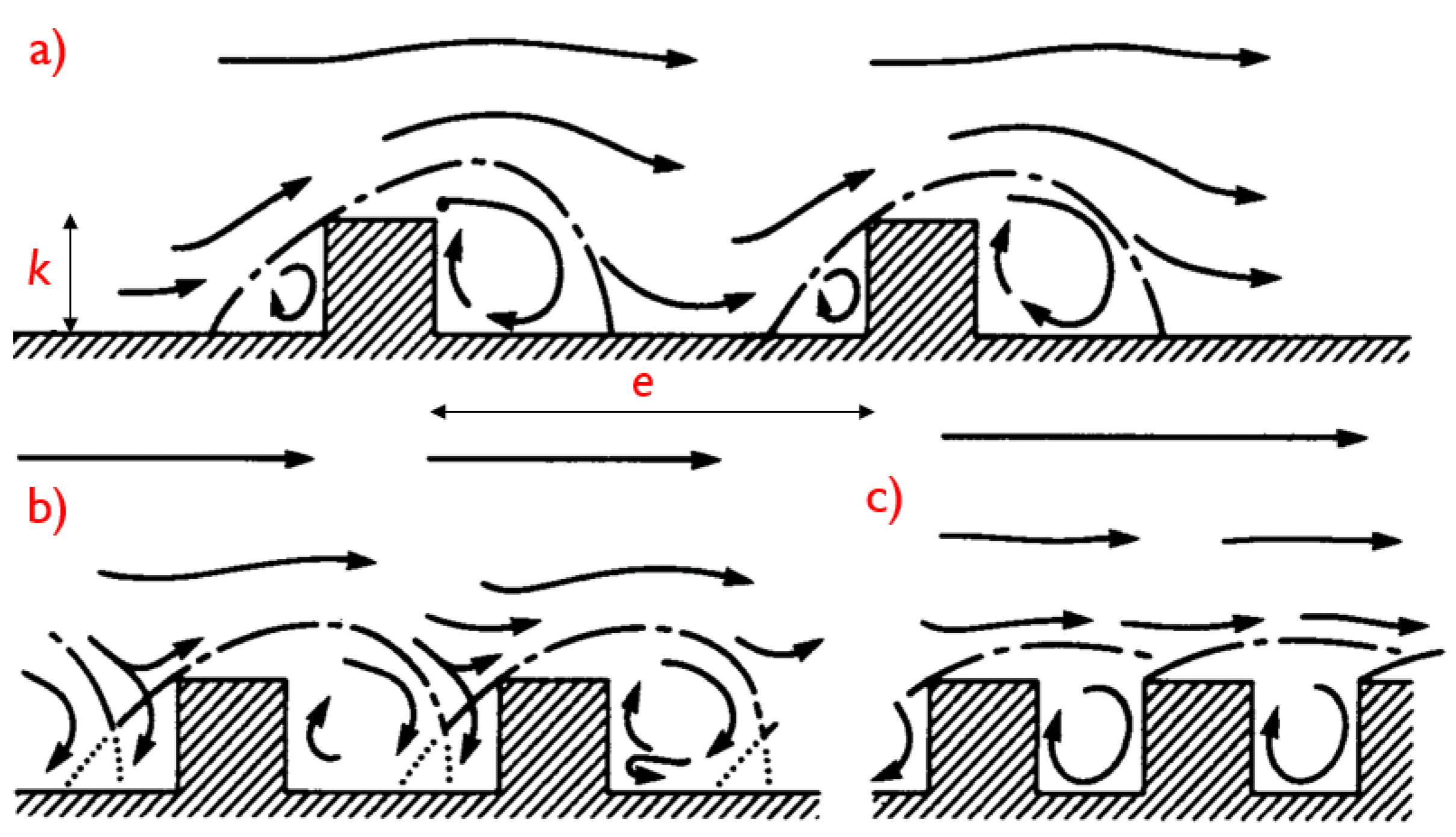
Figure 2.
Some images of the experimental set-up. a) Schematic view of the flume and its components, b) a view of the cylinders used to build the arrays, and c) shows the positions of the ultrasound probes used for the depth measurements.
Figure 2.
Some images of the experimental set-up. a) Schematic view of the flume and its components, b) a view of the cylinders used to build the arrays, and c) shows the positions of the ultrasound probes used for the depth measurements.
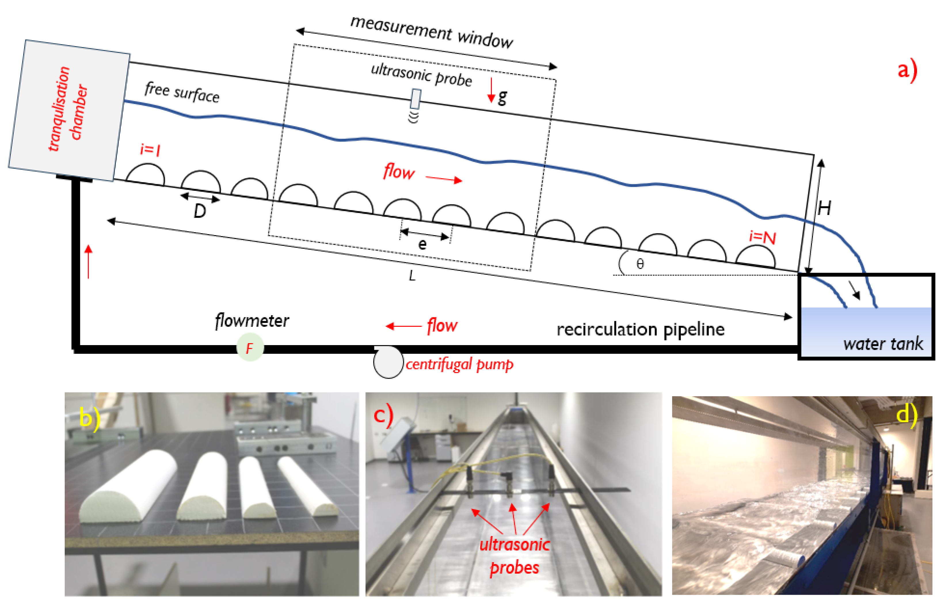
Figure 3.
Flow’s free surface deformation for increasing flow rates, and cylinders of radius 25 mm. a)3.0Ls−1, b)6.0Ls−1, and c)15.0Ls−1. The different deformation patterns can be observed from one experiment, to another. As expected, while Q increases, the normal height also does it. The valleys and peaks of each profile were also included.
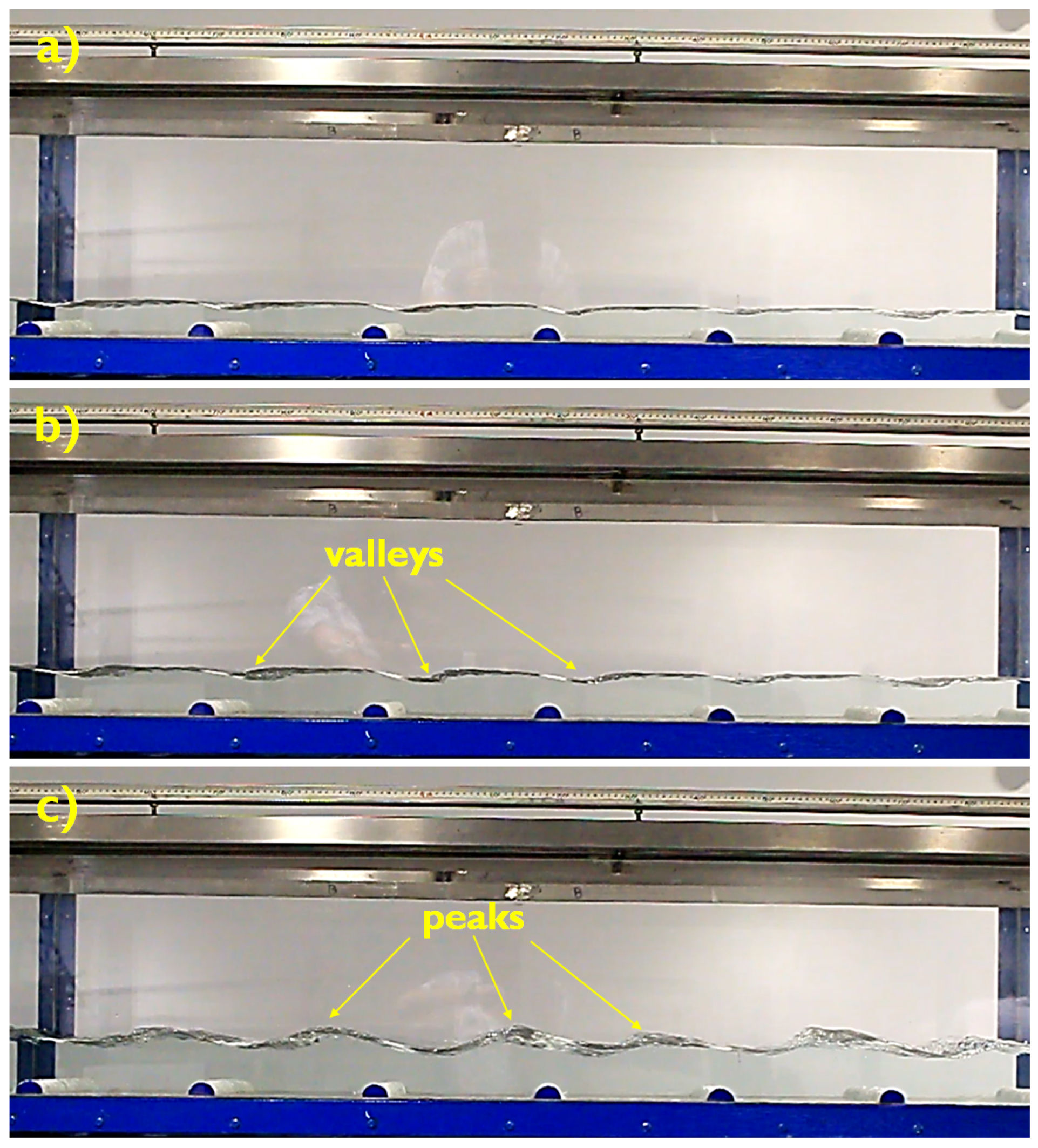
Figure 4.
Flow’s free surface deformation for and increasing size of the cylinders, for a)20 mm, b)35 mm, and c).
Figure 4.
Flow’s free surface deformation for and increasing size of the cylinders, for a)20 mm, b)35 mm, and c).
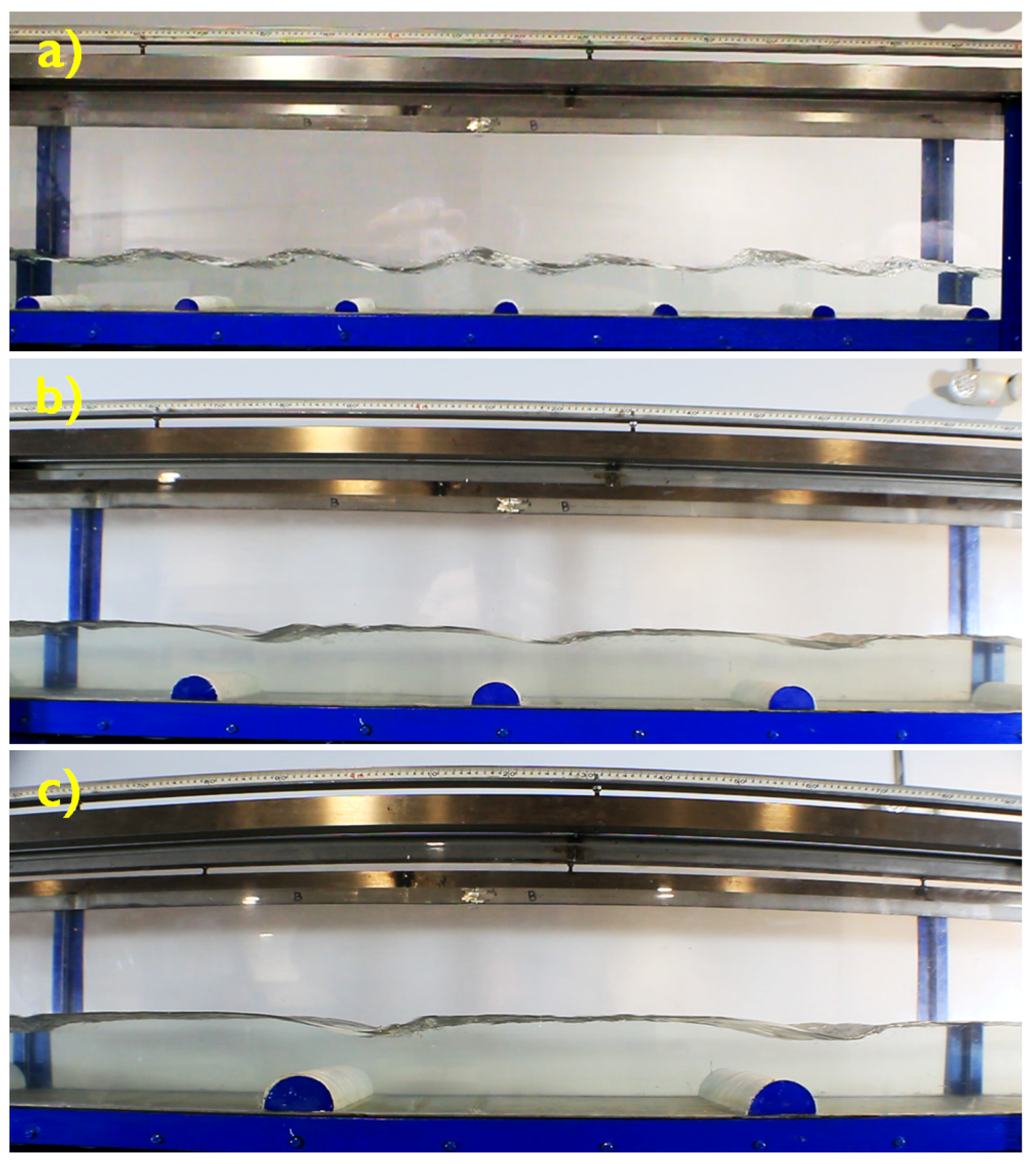
Figure 5.
Evolution of the surface waves observed for the experiment and 25mm. The sequence was taken during a cycle of duration . The red arrow points the peak position observed in one of the waves, from its maximal amplitude to its "death", repeating this cycle after .
Figure 5.
Evolution of the surface waves observed for the experiment and 25mm. The sequence was taken during a cycle of duration . The red arrow points the peak position observed in one of the waves, from its maximal amplitude to its "death", repeating this cycle after .
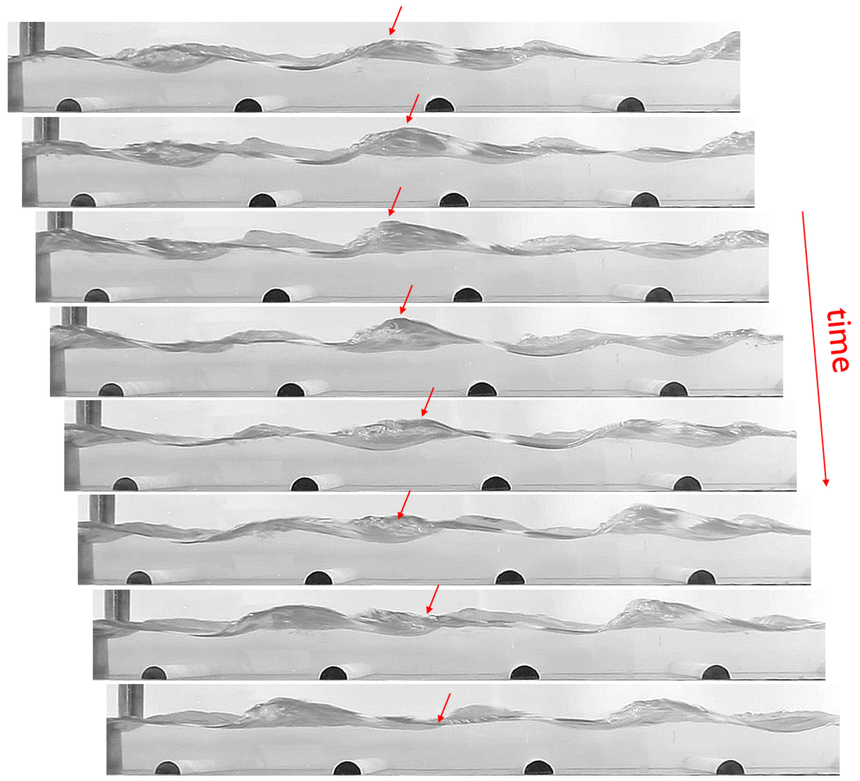
Figure 6.
Backwater profiles obtained for , and radius a)20mm, b)25mm, c)35mm, and d)50mm. In a) the normal depth and the amplitude were included, where is the streamwise average of the valleys and peaks of each profile, respectively.
Figure 6.
Backwater profiles obtained for , and radius a)20mm, b)25mm, c)35mm, and d)50mm. In a) the normal depth and the amplitude were included, where is the streamwise average of the valleys and peaks of each profile, respectively.
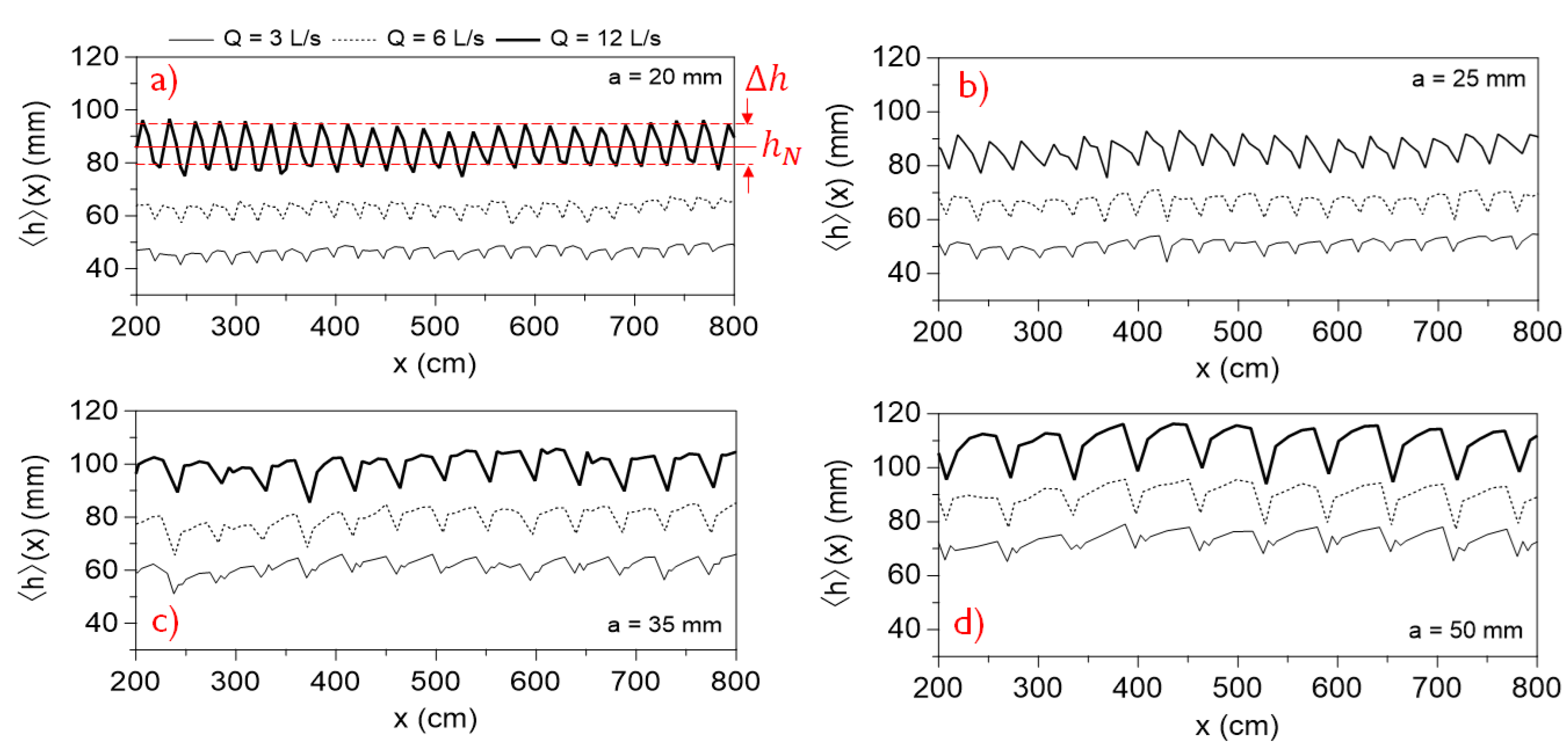
Figure 7.
Relative average deformation of the free surface versus a), b), and b) for different arrays of cylinders.
Figure 7.
Relative average deformation of the free surface versus a), b), and b) for different arrays of cylinders.
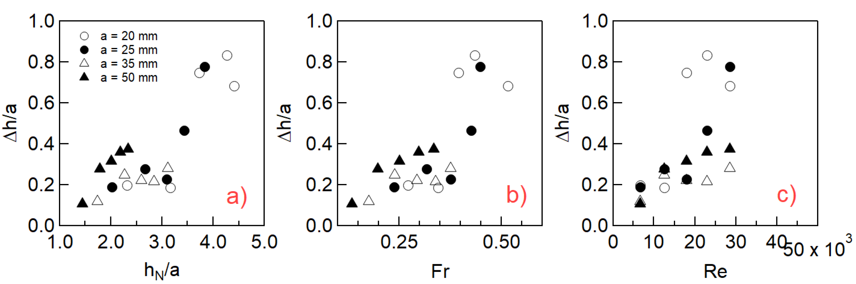
Figure 8.
a) Relative depth vs. for all the experiments. The inset compares the flow depth vs. for the same dataset. b) vs. the streamwise Froude number (this last one from Eq.9), for all the arrays. c) and d) Parameters versus a.
Figure 8.
a) Relative depth vs. for all the experiments. The inset compares the flow depth vs. for the same dataset. b) vs. the streamwise Froude number (this last one from Eq.9), for all the arrays. c) and d) Parameters versus a.
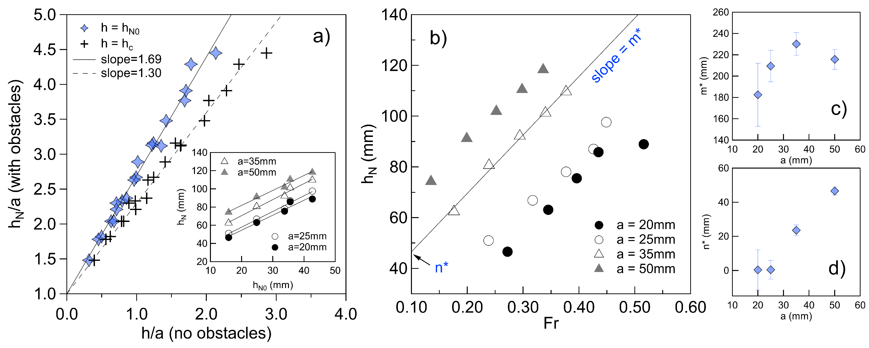
Figure 9.
a) versus for different cylinders. The fitting curve is the Eq.12. b) versus , where the fitting lines given by Eq.13, of slope d. c), d) Parameters c and d versus , where . The decreasing fitting lines are the Eqs.14a,b.
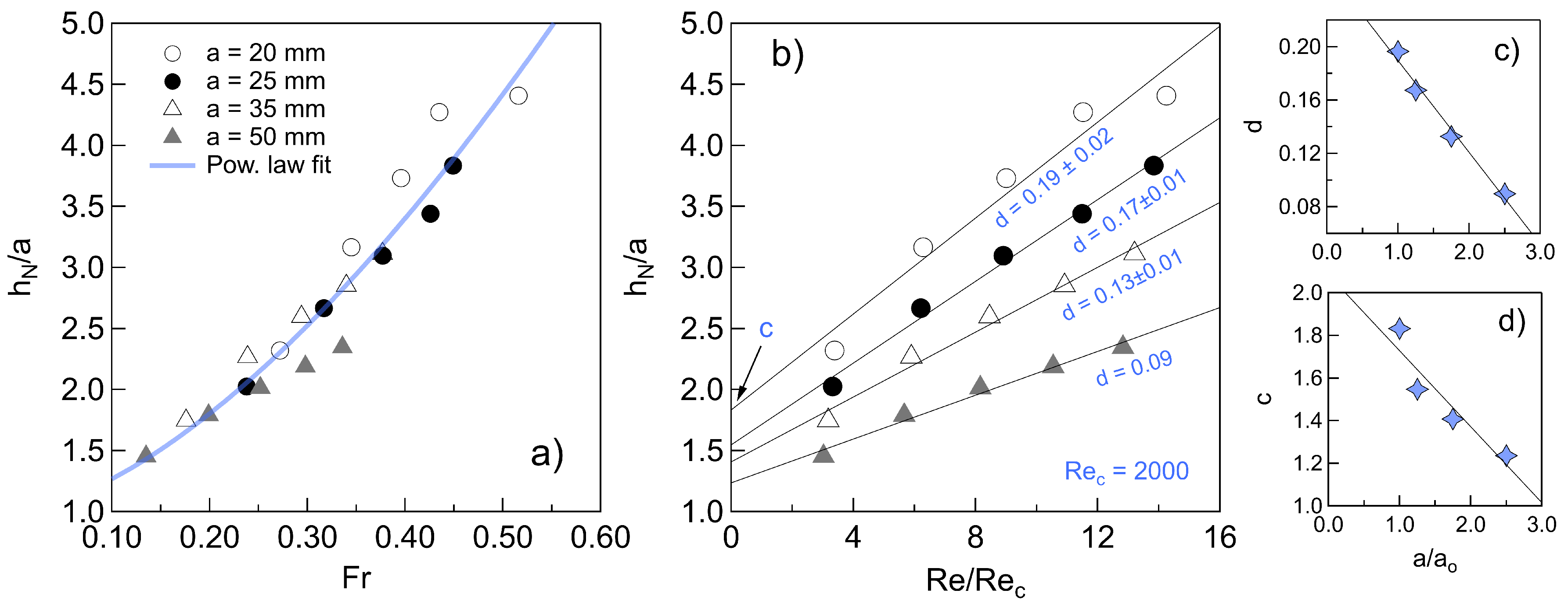
Figure 10.
Distribution of the Darcy friction factor (f) for all the experiments. a) versus . The continuous curve is the Eq.15. Lawrence’s fitting curves (Eqs.2-3), and Colebrook - White formula (Eq.16) were drawn for reference. The inset plots the curve f vs. according to Eq.17). b)f vs. . The continuous curves is given by Eq.18. The empirical parameters were plot against in the insets. Symbols are the same across the chart.
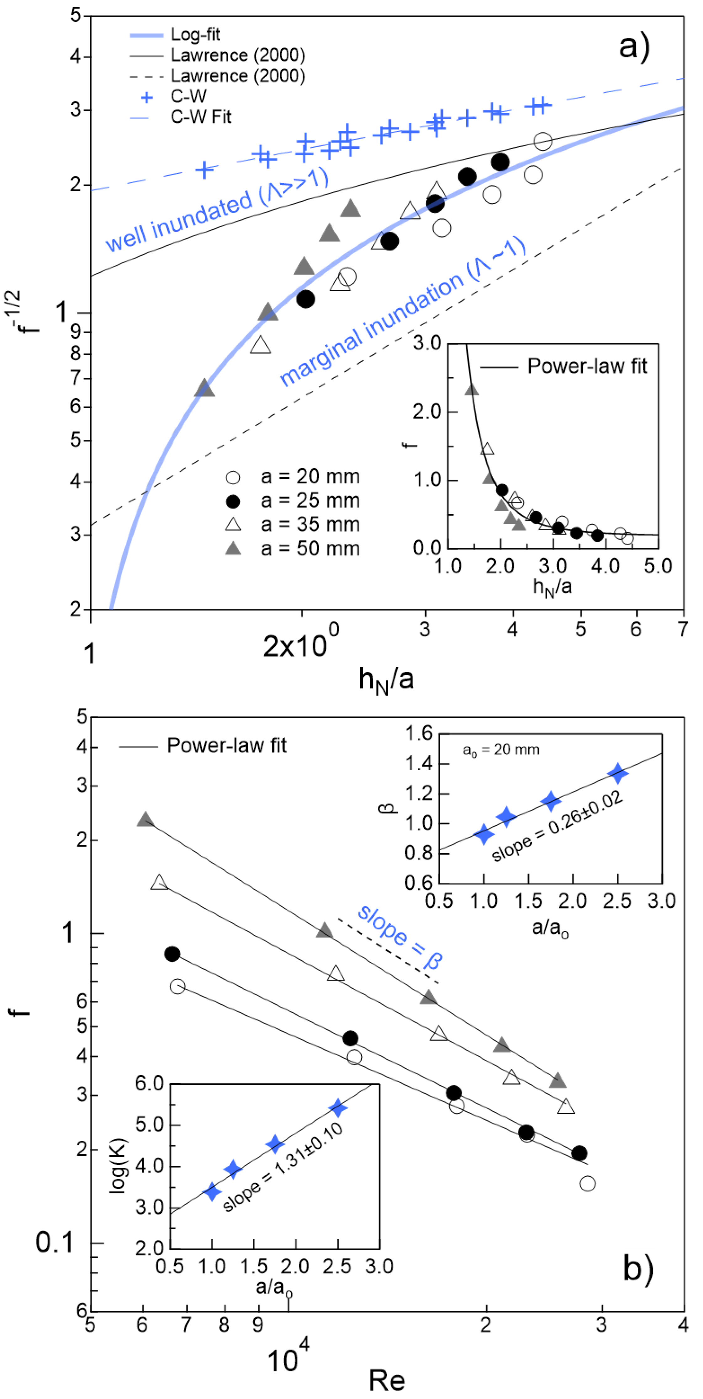
Figure 11.
Distribution of the Manning’s roughness coefficient according to Eq.20. From the fitting lines to the curves vs. , an average roughness coefficient was obtained from the slope of every array. The inset plots vs. .
Figure 11.
Distribution of the Manning’s roughness coefficient according to Eq.20. From the fitting lines to the curves vs. , an average roughness coefficient was obtained from the slope of every array. The inset plots vs. .
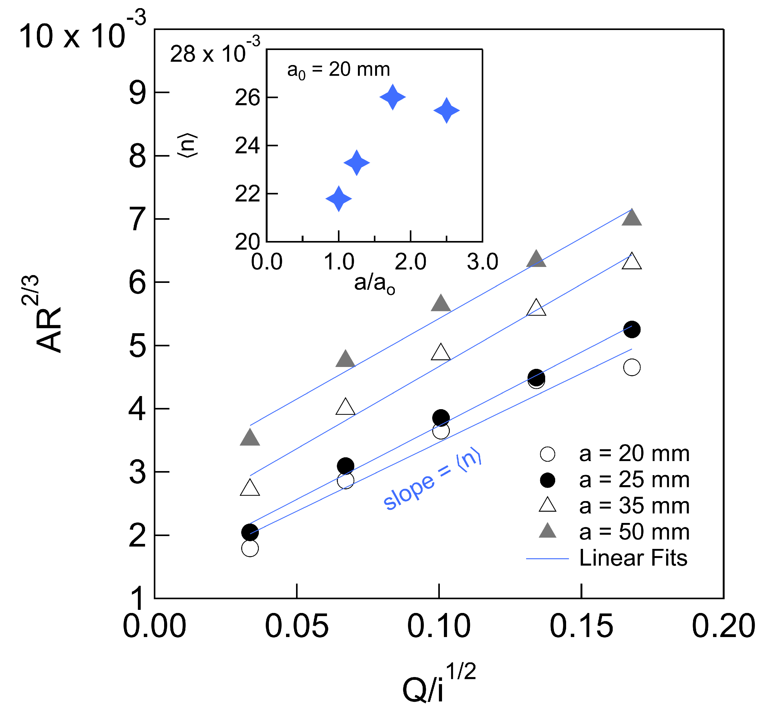
Figure 12.
Scheme adopted for the definition of the parameter .
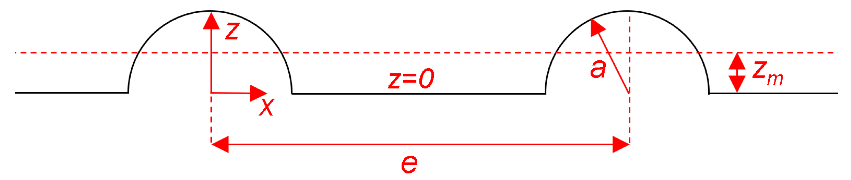
Figure 13.
A scaling law for the Manning roughness coefficient. a) Comparison vs. n for all the runs. b) Comparison vs. . c) Plot of vs. . The central fitting line is given by Eq.25. All the poins fall into a scattering band. A unitary slope was drawn as a guide to the eye. The inset plots the parameter vs. a. The slope of the fitting line is .
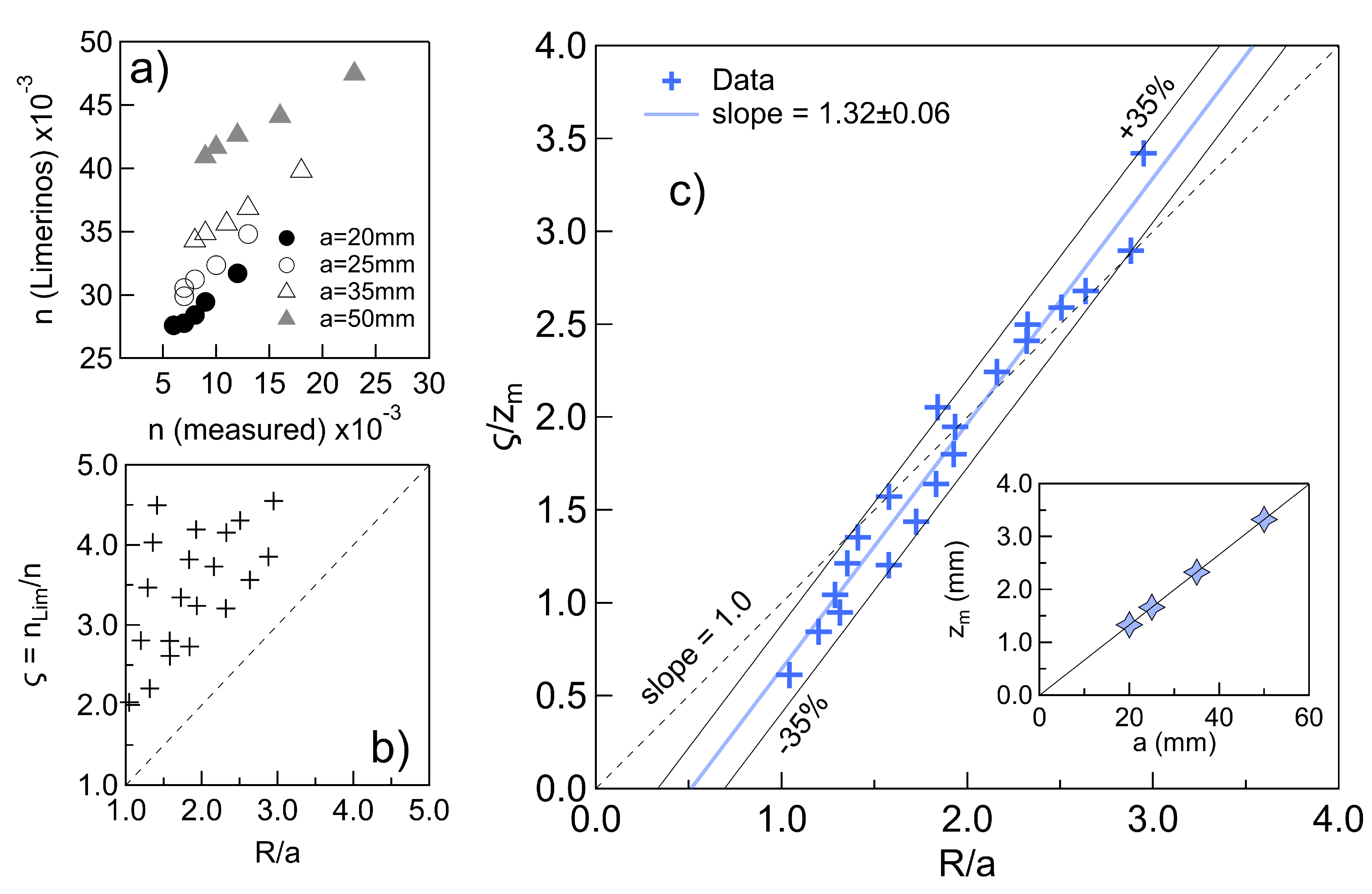

Table 1.
Experimental arrays of the study, where a is the cylinder radius, e the spacing between elements and N the total number of them. The range of variation of the normal depth was included.
Table 1.
Experimental arrays of the study, where a is the cylinder radius, e the spacing between elements and N the total number of them. The range of variation of the normal depth was included.
| Array | a | e | N | |
|---|---|---|---|---|
| (mm) | (mm) | - | (mm) | |
| 1 | 20.0 | 255.3 | 39 | 46.4 - 88.1 |
| 2 | 25.0 | 319.1 | 31 | 50.6 - 95.9 |
| 3 | 35.0 | 446.7 | 22 | 61.1 - 108.9 |
| 4 | 50.0 | 638.2 | 16 | 72.6 - 117.3 |
Disclaimer/Publisher’s Note: The statements, opinions and data contained in all publications are solely those of the individual author(s) and contributor(s) and not of MDPI and/or the editor(s). MDPI and/or the editor(s) disclaim responsibility for any injury to people or property resulting from any ideas, methods, instructions or products referred to in the content. |
© 2025 by the authors. Licensee MDPI, Basel, Switzerland. This article is an open access article distributed under the terms and conditions of the Creative Commons Attribution (CC BY) license (http://creativecommons.org/licenses/by/4.0/).
Copyright: This open access article is published under a Creative Commons CC BY 4.0 license, which permit the free download, distribution, and reuse, provided that the author and preprint are cited in any reuse.


