
Submitted:
10 February 2025
Posted:
11 February 2025
You are already at the latest version
Abstract
The different forms of power functions will be studied in connection with the unified fractional derivative and their Fourier transform computed. In particular, one-sided, even, and odd powers will be studied.
Keywords:
Unified fractional derivative
; two-sided derivative
; power function
MSC: 26A33; 58C05
1. Introduction
The concept of unified fractional derivative (UFD) seems to be introduced by Ortigueira & Trujillo [1] to generalize and unify the notions of one-sided causal/anti-causal (Grünwald-Letnikov) and the two-sided (centred) derivatives [2,3]. Such idea was recovered by Ortigueira & Machado in [4] to introduce fractional derivatives in the context of system theory as part of the movement for coherent definition of fractional derivatives. This led to a deep study in [5] and to generalizations as the tempered derivatives [6,7]. The underlying theory of unified fractional derivative allowed the introduction of formulations in such a way that derivatives/anti-derivatives of any real order could be defined while keeping full coherence with classical results. Namely, as they are shift-invariant, they allow us to define many useful systems, assuming the ARMA form [8] or the diffusion/telegraph form [9,10,11,12,13,14], for Example.
In dealing with shift-invariant linear systems, the exponential functions are their eigenfunctions [8,15,16,17,18]. However, for expressing the impulse and step responses the main role is played by the power functions [18,19]. Their presence/absence is connected with the short and long memory of the system at hand [8,20,21,22,23]. They assume two interlaced aspects: unilateral (tied with causality) and bilateral. Recently, a brief study of some aspects of these functions was done [24], but leaving some unanswered questions. In this paper, we have tried to give an exhaustive presentation of the different expressions of the power functions, their derivatives, and Fourier transforms in relation with particular cases of the UFD.
The paper outlines as follows. In the Section 2, we will describe some useful mathematical tools. The unified fractional derivative will be presented in Section 3, where some of its properties will be introduced. The main objectives of this paper will be treated in Section 4. We will consider the different forms of the power functions and their Fourier transforms. Products by other functions will also be treated. A conjecture about the extrema of functions is also reminded. Finally, some conclusions will be drawn.
2. Some Mathematical Tools
2.1. Laplace and Fourier Transforms
Definition 1.
The direct Laplace transform is defined by:
and the inverse reads
where The right hand side represents the Bromwich integral.
Under suitable conditions, the integral in (1) converges absolutely and uniformly in a vertical strip in the complex plane defined by , where is analytic. This strip is called region of convergence (ROC), and the values of the constants a and b are the abscissas of convergence. It is possible to show that the inversion integral (1), with converges to the half sum of the lateral values, that is, , for any [15,16,25].
If the ROC includes the imaginary axis or this is one of the boundaries, we can substitute getting the Fourier transform by
which are called analysis and synthesis equations, respectively. The integration must be taken in the sense of the Cauchy principal value. The function in (3) is the direct FT, while given by (4) is the inverse FT. About the existence of the FT (3) we can say that if is piecewise continuous, with bounded variation, and absolutely integrable (AI), then the FT exists and the convergence of the integral in (3) is uniform on [15,16].
2.2. On the Distributions
Definition 2.
Let be a continuous function, defined on and null for (in abusive language, we call it causal function, by analogy with the impulse response of causal systems). Sometimes the designation “right function” is also used. Represent the usual derivative by D. We define a distribution as a derivative of a given order of
Several mathematical formulations support this definition and extend the validity of the LT and FT [25,26,27,28,29], but this is out of our objectives.
Example 1.
Example 2.
Let . We define the causal fractional power function by
where the Gamma function is given by
for .
The Laplace transform of reads [30]
We can prove that, in the context of Laplace or Fourier transforms, the convolution of two distributions gives rise to another distribution [25,28,29,35,36]. In such cases, is the neutral element of the convolution and, if and are convolutionally inverse, then
The inversion of this convolution has been subject of many publications [37,38]. The causal case, mainly based in the Abel’s algorithm, has attracted the attention recently [22,39,40,41,42].
Remark 1.
In this paper we deal with the multivalued expression . To define a function we have to fix a branch cut line and choose a branch (Riemann surface). To deal with right functions a simple correct procedure consists of choosing the negative real half-axis as branch cut line and adopting the principal branch; we assume also that the obtained function is continuous above the branch cut line, so that .
2.3. On the Binomial Coefficients
The importance of the binomial coefficients sequence is unquestionable [43,44,45,46]. In our applications we express them in the form:
where, if then with is the Pochhammer symbol for the raising factorial that can be written as
Remark 2.
It is important to emphasize the fact that this representation of the binomial coefficients avoids the use of the gamma function, simplifying computations.
The absolute value of sequence represented in (11) is increasing for , constant for and decreasing for . It can be shown that it varies asymptotically as [46]. It is finite, if . These expressions allow us to recover well-known characteristics of the binomial series. Let . The binomial series reads
This series converges absolutely and uniformly for any provided that [43,46]. If the series diverges except when is a non-negative integer, in which case the series becomes a finite sum. However, we are interested in the case about which we can say that
- the series converges absolutely if and only if ;
- if , the series converges simply, if and only if ;
- if the series diverges for .
The relation (12) allows us to obtain an interesting bilateral binomial series, defined on the unit circle, and given by [3]
where and . It is a simple matter to verify that the coefficients of this series result from the cross-correlation of the binomial coefficients corresponding to orders a and b [3,47]:
3. The Unified Fractional Derivative
Definition 3.
The operator whose associated frequency response, , given by
verifying
is named unified fractional derivative [1,4]; α is the derivative order and θ the asymmetry parameter.
When , we will omit the parameter, In particular, we set,
This definition has a deep connection with the Fourier transform and allows us to extend two dual properties [48].
Theorem 1.
Let be the Fourier transform of a given function or distribution . Then, the UFD of is given by
This is a consequence of (15). The dual is obtained immediately
Remark 3.
• The above definition is very general. Given a pair, (), there exists, at least, one explicit description of the UFD. Suitable choices allow us to recover the causal, anti-causal, and bilateral derivatives. The particular, most interesting, cases are [5]
- –
- –
- — Riesz derivative [52].
- –
-
- The Bode amplitude diagram is a straight line with slope ;
- The Bode phase is an horizontal straight line with ordinate
- Due to the properties of the Fourier transform, the UFD verifies all the required items for really being a fractional derivative [56];
- We must be careful when using (17), since the hermitian property can be lost for some values of the asymmetry parameter.
-
Additivity and commutativity of the ordersIn applying this property it is convenient to have in mind the periodicity in .as we observe from (14). It is a simple task to verify thatTherefore, we can writeThese relations motivate the introduction of two series analog to Mittag-Leffler’s that may be useful in solving partial differential equations involving space derivatives. They readand
-
Existence of inverse derivativeWe define the identity operatorFrom this definition and (18), the anti-derivative exists when and . Therefore,It is interesting to note thatRemark 4. We must highlight the difference between anti-derivative and primitive. This one is the right inverse of the derivative, while the anti-derivative is the left and right inverse.
-
Hermitian/anti-hermitian decompositionvalid for any pairs . This property is important enough to demand for its deduction. As , we havethat leads to (22).The hermitian part is obtained fromIts FT inverse is the impulse response of the Riesz derivative [5]. Similarly, the anti-hermitian isIts impulse response defines the Feller derivative [5].
-
Causal/anti-causal decompositionConsider the last two relations and choose , so that . Thenandwhich imply, respectivelyandThese expressions lead toshowing how the UFD can be expressed in terms of the Liouville causal and anti-causal derivatives.
Remark 5.
- Riesz + Feller derivatives;
- Liouville causal + anti-causal derivatives.
Besides the two sets of derivatives are inter-related.
4. Power Functions and Their Derivatives
4.1. Types of Powers
In the previous section, we showed that we can express the UFD as linear combinations of causal/anti-causal or hermitian/anti-hermitian derivatives. The former are defined by right/left impulse responses, while the later by symmetric/anti-symmetric ones. In fact, we have to relate the power frequency responses and the time power functions. Such frequency responses are
- Causal Liouville –
- Anti-causal Liouville –
- Hermitian Riesz –
- Anti-Hermitian Feller –
They have correspondence with powers of types
- Right –
- Left –
- Symmetric (even) –
- Anti-symmetric (odd) –
Therefore, we will consider preferably Liouville (and Grünwald-Letnikov), Riesz, and Feller derivatives.
4.2. – Liouville
The cases underly the causal/anti-causal derivatives. We will treat the causal only, since the anti-causal instances will be obtained from the corresponding causal through a change
Therefore, we are going to look for the inverse FT of the frequency response
As referred above, we omitted the reference to . This expression deserves a careful analysis.
- If , the function is hermitian. Therefore, its inverse FT is a real function, neither even, nor odd. It will be deduced below.
-
When we have two situations corresponding to even and odd orders. If N is even, is real even; the same happens to the FT inverse. If N is odd, is imaginary odd and its inverse is real odd. In fact it is known that this case is singular, sinceMoreover, it can be written as [26]expressed in a form that is coherent with the general expression, as we will se below.
- If the order is a negative integer, has also an alternancy real/imaginary giving even/odd FT inverses, therefore bilateral functions (no causality). This case will be treated later.
As observed looking into the items, we were driven into a distribution framework and delt with pseudo-functions [28]. We tried to establish a direct relation between the frequency response and the causal behaviour. As we verified, such a correspondence only happens when the order is not integer. In such cases, we can show that [46,57,58]
where , the greatest integer less than or equal to . If the summation is null.
Attending to the observations we made above, we conclude that there exists what we can consider as generalized impulse response of the derivative defined by the frequency response . If is not a negative integer number, such an impulse response assumes the form
being a pseudo-function when . Having this in mind we are going to make a brief study of this distribution, by computing it from the derivative definition (30). This objective can be achieved through some manipulations in the definition of GL, using a procedure that follows the one used in [59]. We reduce the difficulties by working with the step response. We know that
then the impulse response, , verifies
where
Attending to these relations and using (35) we obtain
We are going to look into this result from a deeper point of view by computing it directly from the GL causal derivative. This one is got from (30) by setting
Theorem 2.
Let and . Then
For a simple proof, let . We get
However, [46]
A well-known property of the gamma function [46] gives
for larger values of L. Therefore,
that leads to the expected result. This Theorem deserves some comments:
- It is valid for any real order;
- For it leads to the well-known resultthat corresponds to a recursive computation of the anti-derivative;
- If , we getas we showed above.
This Theorem confirms the correctness of (35).
A similar procedure was used by Miller & Ross [59] to obtain
Corollary 1.
The α–order derivative of the power function is given by
for any real α.
From these results and property (18) we can generalize the previous relation to obtain, for any real [60],
Remark 6.
This relation shows something very important: given a power of the type the sequence of order β derivatives does not stop
This highlights the abnormality of the Caputo derivative that stops for , since a null derivative of the Heaviside function is obtained.
We showed that any causal power function can be considered as a fractional derivative of a suitable order of the Heaviside function
However, this does not mean that all the versions result from inverting . In fact, we showed that
if This result leaves out the positive integer order power function because its FT is not given by a simple expression like . In fact, it is not very hard to show that [26,29]
Using the property (17) with we obtain
and so,
Thus an “abnormal” term appears when comparing with (44). Therefore, the inverse FT of is not causal.
Another interesting result can be formulated as
4.3. – Riesz and Feller Cases
With , we are led to what we can call Riesz and Feller derivatives, respectively. From Theorem 1 we get the corresponding frequency responses
and
From the properties of FT, we know that the corresponding impulse responses, and , are even and odd, respectively. Recovering the impulse response we got in the previous subsection and using the relations (25) and (26), we deduce
Theorem 4.
Let The impulse responses, and , are given by
and
This result comes from inserting (35) into (27) and (28). Of course, we must be careful with the singular cases that appear when . We are going to study each case step by step. Consider the case. We have 4 noteworthy cases: positive/negative and even/odd Let .
4.3.1. Riesz Case
-
.We have,and
-
.This case is not singular. We obtain directly
-
.We note thatthat gives
-
.In this case, the term creates difficulties. We need another approach. We will treat it below.
4.3.2. Feller Case
In the Feller case, we get
-
.Note that,which gives
-
.This case is singular. We leave it for now.
-
.Using (54), we obtain
-
.This case does not have any difficulty. We have
Remark 7.
Till now, we left unsolved three problems consisting in the inversion of . We know already how to solve the first. Consider the with a non solved case in the previous subsection. We must make a distinction between the even and odd cases that will come from (51) and (57) respectively, leading to
and
Therefore, the inverse of is one of the previous relation. At this time, we do not know how to get and To get them, we need another approach that we will describe in a later section [5].
We can resume the FT inversions we made till now, by constructing the following Table 1.
4.3.3. Derivatives of the Power Functions
Given the above relationships and an appropriate change in the parameters, we obtain the derivatives of the power functions. We consider regular cases (orders not equal to negative integers). The others are obtained from the Table 1. Let . We get:
-
Therefore,
- With identical procedure we get successively
From these relations, we conclude that, while the Riesz derivative keeps the symmetry characteristic of the power, the Feller inverts it. In fact
- The Riesz derivative of a symmetric/anti-symmetric power is symmetric;
- The Feller derivative of a symmetric/anti-symmetric power is anti-symmetric/symmetric.
Therefore, if we compute the bilateral derivative of a symmetric power for constant order, but varying from 0 to 1, we move from symmetry to anti-symmetry, passing through all the intermmediate asymmetric powers, because
From this result, we can conclude that, if , the form of the power function on the right depends essentially on the asymmetry parameter. It is not very difficult to deduce the formula for and relate it with (64).
Definition 4.
Theorem 5.
In agreement with definition 4, there are two (quadrature) filters with frequency responses, and that transform a given asymmetric power function into a symmetric and anti-symmetric powers respectively. They are given by
and
where a is any real value. In particular, we can set , so that the two filters are generalized Hilbert transforms.
This led us to formulate the following conjecture [61].
Conjecture 1.
Let be a piecewise continuous bounded function defined on having Fourier transform. Assume it has an extremum at . Then, there are derivative orders, and one asymmetry parameter such that the unified fractional derivative, , is null.
To understand it and check its plausibility, let and suppose that
in an interval . In such a situation, attending to the Theorem 5, the derivative, is null at . As it is clear, the derivative has a maximum at that point.
4.4. Remaining Cases
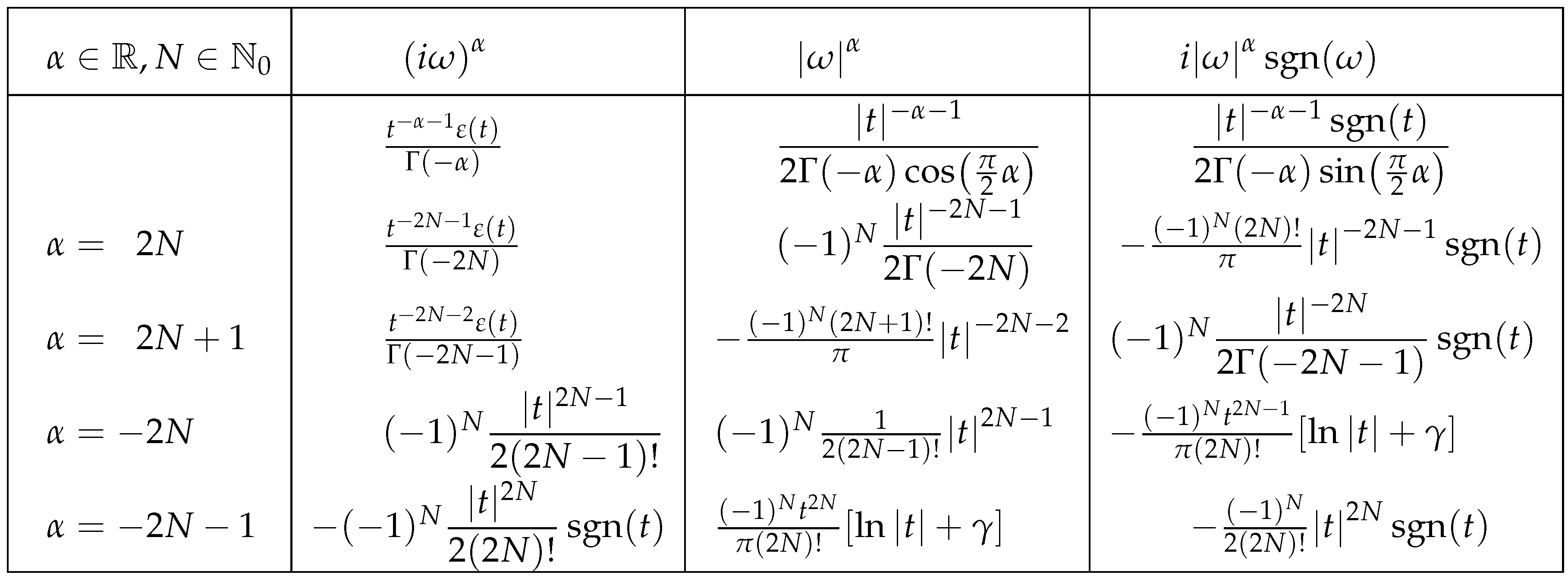
4.4.1. Other Singular Powers
In the above subsection we left unsolved two cases corresponding to the FT inversions of the transforms . These express “abnormal” cases that cannot be deduced directly from the general formulae (48) and (49). In [5] the solutions were found through a small trick consisting in doind the ordinary derivation relatively to the fractional order, followed by some simple manipulations. We are led to
and
Therefore we can perform the completition of the above table.
With this table, we can solve some open problems, as the application of mixed Liouville/Riesz-Feller or the computation of the FT of some integer powers.
4.4.2. The Liouville Derivative of Two-Sided Power Functions
In [24], the computation of the Liouville derivative of was addressed and a partial solution was obtained. We have two ways of solving the problem: using the regularized Liouville derivative or through the FT as we did above. In the first case, we are limited by the properties of the gamma and beta integrals that introduce some limitations, although the regularization allows an enlargement of the parameter domains [58]. However, we cannot obtain the derivative of an increasing power, Using the FT, we can solve the problem with greater generality. We will consider the non integer case only. Let . The FT of is obtained from
applying the duality property
Write successively
Therefore, using (48) with (52) and (49) with (54), we get
So,
We can simplify this result as
Remark 8.
It is important to note that
4.4.3. The Fourier Transform of Negative Integer Powers
The presence of the gamma function can produce a major change in the characteristics of a power. For Example, is a delta distribution, while is a hyperbola. Obviously, the corresponding FT are deeply different. The use of Table 2 and the duality property give the FT of some negative power functions. Let . We have 4 cases
-
Using Table 2 we obtainFrom this relation, we can write
-
In the referred table, we findthat gives
4.5. Products of Powers and Other Functions
In some practical applications, we need to find fractional derivatives of the product of power functions and logarithms. We are going to find closed formulae and the corresponding FT. It is a simple task to get such formulae: we only have to pick those we described in the previous Section and compute suitable derivatives relatively to any involved parameter. This can be done both in time or frequency domains. Depending on the used derivative we can obtain several formulae starting from one. The first interesting result can be formulated as
Theorem 6.
In particular, with , we obtain
Theorem 7.
Consider relation (60) and proceed as above, computing the ordinary derivative relatively to μ.
with
and
More interesting in applications is the multiplication of powers and exponentials [6].
Theorem 8.
Consider the product , where . This function is important in solving linear systems and, in particular, for defining tempered derivatives and systems. The Liouville derivative of is given by
The proof is immediate from the Leibniz rule
by using the relations introduced in Section 3. If, instead of a bilateral power, we used a causal one, the summation would have infinite terms. Let . This case is interesting, because we can associate the Heaviside function to the power or to the exponential, giving two different expressions
-
We can compute either from the Taylor expansion of the exponential, or from the Liouville integral.
5. Conclusion
We introduced the general forms of power functions, computed their derivatives, and found their Fourier transforms. The unified fractional derivative was used, due to its connection with the powers.
Funding
The author was partially funded by National Funds through the Foundation for Science and Technology of Portugal, under projects UIDB/00066/2020.
Data Availability Statement
No new data were created or analyzed in this study. Data sharing is not applicable to this article.
Conflicts of Interest
The author declares no conflicts of interest.
References
- Ortigueira, M.D.; Trujillo, J.J. A unified approach to fractional derivatives. Communications in Nonlinear Science and Numerical Simulation 2012, 17, 5151–5157. [Google Scholar] [CrossRef]
- Ortigueira, M.D. Riesz potential operators and inverses via fractional centred derivatives. Int. J. Math. Mathematical Sciences 2006, 2006, 48391:1–48391:12. [Google Scholar] [CrossRef]
- Ortigueira, M.D. Fractional central differences and derivatives. Journal of Vibration and Control 2008, 14, 1255–1266. [Google Scholar] [CrossRef]
- Ortigueira, M.D.; Machado, J.A.T. Fractional Derivatives: The Perspective of System Theory. Mathematics 2019, 7. [Google Scholar] [CrossRef]
- Ortigueira, M.D. Two-sided and regularised Riesz-Feller derivatives. Mathematical Methods in the Applied Sciences 2021, 44, 8057–8069. [Google Scholar] [CrossRef]
- Ortigueira, M.D.; Bengochea, G.; Machado, J.A.T. Substantial, tempered, and shifted fractional derivatives: Three faces of a tetrahedron. Mathematical Methods in the Applied Sciences 2021, 44, 9191–9209. [Google Scholar] [CrossRef]
- Ortigueira, M.D.; Bengochea, G. Bilateral tempered fractional derivatives. Symmetry 2021, 13, 823. [Google Scholar] [CrossRef]
- Ortigueira, M.D.; Machado, J.T. The 21st century systems: An updated vision of continuous-time fractional models. IEEE Circuits and Systems Magazine 2022, 22, 36–56. [Google Scholar] [CrossRef]
- Machado, J.T. And I say to myself: “What a fractional world!”. Fractional Calculus and Applied Analysis 2011, 14, 635–654. [Google Scholar] [CrossRef]
- Machado, J.T.; Galhano, A.M.; Trujillo, J.J. On Development of Fractional Calculus During the Last Fifty Years. Scientometrics 2014, 98, 577–582. [Google Scholar] [CrossRef]
- Herrmann, R. Fractional Calculus, 3rd ed.; World Scientific: Singapore, 2018. [Google Scholar]
- Teodoro, G.S.; Machado, J.T.; De Oliveira, E.C. A review of definitions of fractional derivatives and other operators. Journal of Computational Physics 2019, 388, 195–208. [Google Scholar] [CrossRef]
- Mainardi, F. Fractional calculus and waves in linear viscoelasticity: an introduction to mathematical models; World Scientific: Singapore, 2022. [Google Scholar]
- Ortigueira, M.D. An entropy paradox free fractional diffusion equation. Fractal and Fractional 2021, 5, 236. [Google Scholar] [CrossRef]
- Oppenheim, A.V.; Willsky, A.S.; Hamid, S. Signals and Systems, 2nd ed.; Prentice-Hall: Upper Saddle River, NJ, 1997. [Google Scholar]
- Roberts, M. Fundamentals of signals and systems; McGraw-Hill Science/Engineering/Math: New York, 2007. [Google Scholar]
- Valério, D.; da Costa, J.S. An Introduction to Fractional Control; Control Engineering, IET: Stevenage, 2012. [Google Scholar]
- Valério, D.; Ortigueira, M.D. Variable-Order Fractional Scale Calculus. Mathematics 2023, 11, 4549. [Google Scholar] [CrossRef]
- Machado, J.T.; Pinto, C.M.; Lopes, A.M. A review on the characterization of signals and systems by power law distributions. Signal Processing 2015, 107, 246–253. [Google Scholar] [CrossRef]
- Sonine, N. On differentiation of an arbitrary order (in Russian. Mat. Sb. 1872, 6, 1–38. [Google Scholar]
- Sonine, N. Sur la généralisation d’une formule d’Abel. Acta Math. 1884, 4, 171–176. [Google Scholar] [CrossRef]
- Tarasov, V.E. Multi-kernel general fractional calculus of arbitrary order. Mathematics 2023, 11, 1726. [Google Scholar] [CrossRef]
- Luchko, Y. General fractional integrals and derivatives and their applications. Physica D: Nonlinear Phenomena 2023, 133906. [Google Scholar] [CrossRef]
- González-Santander, J.L.; Mainardi, F. Some Fractional Integral and Derivative Formulas Revisited. Mathematics 2024, 12, 2786. [Google Scholar] [CrossRef]
- Zemanian, A.H. Distribution Theory and Transform Analysis: An Introduction to Generalized Functions, with Applications; Lecture Notes in Electrical Engineering, 84; Dover Publications: New York, 1987. [Google Scholar]
- Gelfand, I.M.; Shilov, G.P. Generalized Functions; Academic Press: New York, 1964. [Google Scholar]
- Ferreira, J. Introduction to the Theory of Distributions; Pitman Monographs and Surveys in Pure and Applied Mathematics; Pitman: London, 1997. [Google Scholar]
- Hoskins, R.; Pinto, J. Theories of Generalised Functions: Distributions, Ultradistributions and Other Generalised Functions; Horwood Publishing Limited: Cambridge, 2005. [Google Scholar]
- Hoskins, R. Delta Functions: An Introduction to Generalised Functions; Woodhead Publishing Limited: Cambridge, 2009. [Google Scholar]
- Henrici, P. Applied and Computational Complex Analysis; Wiley-Interscience: New York, 1991; Vol. 2. [Google Scholar]
- Oldham, K.B.; Myland, J.; Spanier, J. An atlas of functions: with equator, the atlas function calculator; Springer: New York, 2009. [Google Scholar]
- Chaudhry, M.A.; Zubair, S.M. On a Class of Incomplete Gamma Functions with Applications; Chapman and Hall/CRC: Boca Raton, 2001. [Google Scholar]
- Olver, F. NIST handbook of mathematical functions. US Department of Commerce, National Institute of Standards and Technology 2010. [Google Scholar]
- Li, C. Several Results of Fractional Derivatives in D’ (R+). Fractional Calculus and Applied Analysis 2015, 18, 192–207. [Google Scholar] [CrossRef]
- Li, C.; Li, C.; Kacsmar, B.; Lacroix, R.; Tilbury, K. The Abel integral equations in distribution. Adv. Anal. 2017, 2, 88–104. [Google Scholar] [CrossRef]
- Zayed, A.I. Handbook of Function and Generalized Function Transformations; CRC press: Boca Raton, 1996. [Google Scholar]
- Hirschman, I.I.; Widder, D.V. The Convolution Transform; Princeton University Press: Princeton, New Jersey, 1955. [Google Scholar]
- Domínguez, A. A History of the Convolution Operation [Retrospectroscope]. IEEE Pulse 2015, 6, 38–49. [Google Scholar] [CrossRef]
- Kochubei, A.N. General Fractional Calculus, Evolution Equations, and Renewal Processes. Integral Equations and Operator Theory 2011, 71, 583–600. [Google Scholar] [CrossRef]
- Luchko, Y.; Yamamoto, M. The general fractional derivative and related fractional differential equations. Mathematics 2020, 8, 2115. [Google Scholar] [CrossRef]
- Hanyga, A. A comment on a controversial issue: A generalized fractional derivative cannot have a regular kernel. Fractional Calculus and Applied Analysis 2020, 23, 211–223. [Google Scholar] [CrossRef]
- Ortigueira, M.D. Searching for Sonin kernels. Fractional Calculus and Applied Analysis 2024, 27, 2219–2247. [Google Scholar] [CrossRef]
- Pollard, H.; Shisha, O. Variations on the binomial series. The American Mathematical Monthly 1972, 79, 495–499. [Google Scholar] [CrossRef]
- Abramowitz, M.; Stegun, I.A. Handbook of mathematical functions with formulas, graphs, and mathematical tables; Dover Publications: New York, 1968; Vol. 55. [Google Scholar]
- Dzhumadil’daev, A.; Yeliussizov, D. Power sums of binomial coefficients. J. Integer Seq 2013, 16, 4. [Google Scholar]
- Samko, S.G.; Kilbas, A.A.; Marichev, O.I. Fractional Integrals and Derivatives; Gordon and Breach: Yverdon, 1993. [Google Scholar]
- Ortigueira, M.D. Introduction to fractional linear systems. Part 2. Discrete-time case. IEE Proceedings - Vision, Image and Signal Processing 2000, 147, 71–78. [Google Scholar] [CrossRef]
- Ortigueira, M.D.; Bengochea, G. On the fractional derivative duality in some transforms. Mathematics 2023, 11, 4464. [Google Scholar] [CrossRef]
- Liouville, J. Memóire sur quelques questions de Géométrie et de Méchanique, et sur un nouveau genre de calcul pour résoudre ces questions. Journal de l’École Polytechnique, Paris 1832, 13, 1–69. [Google Scholar]
- Liouville, J. Memóire sur le calcul des différentielles à indices quelconques. Journal de l’École Polytechnique, Paris 1832, 13, 71–162. [Google Scholar]
- Liouville, J. Note sur une formule pour les différentielles à indices quelconques, à l’occasion d’un Mémoire de M. Tortolini. Journal de mathématiques pures et appliquées 1855, 20, 115–120. [Google Scholar]
- Riesz, M. L’intégrale de Riemann-Liouville et le problème de Cauchy pour l’équation des ondes. Bulletin de la Société Mathématique de France 1939, 67, 153–170. [Google Scholar] [CrossRef]
- Feller, W. On a generalization of Marcel Riesz potentials and the semigroups, generated by them. Communications du seminaire mathematique de universite de Lund 1952, 21, 72–81. [Google Scholar]
- Proakis, J.G.; Manolakis, D.G. Digital signal processing: Principles, algorithms, and applications; Prentice Hall: New Jersey, 2007. [Google Scholar]
- Ortigueira, M.D.; Valério, D. Fractional Signals and Systems; De Gruyter: Berlin, Boston, 2020. [Google Scholar]
- Ortigueira, M.D.; Machado, J.T. What is a fractional derivative? Journal of Computational Physics 2015, 293, 4–13. [Google Scholar] [CrossRef]
- Kilbas, A.A.; Srivastava, H.M.; Trujillo, J.J. Theory and Applications of Fractional Differential Equations; Elsevier: Amsterdam, 2006. [Google Scholar]
- Ortigueira, M.D. A coherent approach to non-integer order derivatives. Signal Processing 2006, 86, 2505–2515. [Google Scholar] [CrossRef]
- Miller, K.; Ross, B. An Introduction to the Fractional Calculus and Fractional Differential Equations; Wiley: New York, 1993. [Google Scholar]
- Ortigueira, M.D. Fractional Calculus for Scientists and Engineers; Lecture Notes in Electrical Engineering; Springer: Dordrecht, Heidelberg, 2011. [Google Scholar]
- Ortigueira, M.D. Finding extrema using the unified fractional derivative: a conjecture. Submitted for publication 2024. [Google Scholar]

Table 1.
Incomplete table with FT inverses.
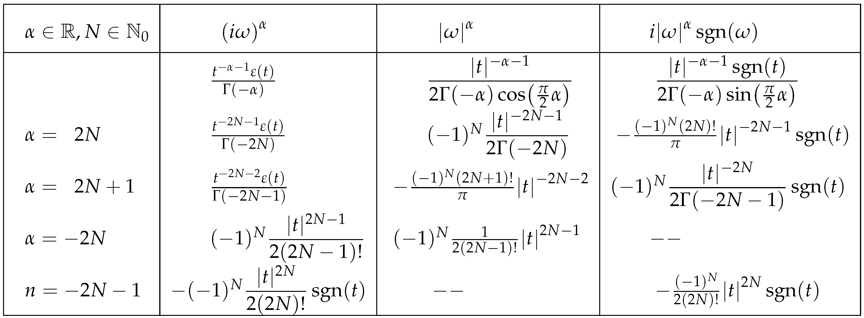
Table 2.
Complete table with FT inverses.
Disclaimer/Publisher’s Note: The statements, opinions and data contained in all publications are solely those of the individual author(s) and contributor(s) and not of MDPI and/or the editor(s). MDPI and/or the editor(s) disclaim responsibility for any injury to people or property resulting from any ideas, methods, instructions or products referred to in the content. |
© 2025 by the authors. Licensee MDPI, Basel, Switzerland. This article is an open access article distributed under the terms and conditions of the Creative Commons Attribution (CC BY) license (http://creativecommons.org/licenses/by/4.0/).
Copyright: This open access article is published under a Creative Commons CC BY 4.0 license, which permit the free download, distribution, and reuse, provided that the author and preprint are cited in any reuse.


