Submitted:
07 February 2025
Posted:
11 February 2025
Read the latest preprint version here
Abstract
Linear classifiers are preferred for some tasks because they overfit less and provide interpretable decision boundaries. Yet, achieving both scalability and predictive performance remains challenging. Here, we propose a theoretical framework named geometric discriminant analysis (GDA). GDA includes the family of linear classifiers that can be expressed as function of a centroid discriminant basis (CDB0) - the connection line between two centroids - adjusted by geometric corrections under different constraints. We demonstrate that linear discriminant analysis (LDA) is a subcase of the GDA theory, and we show its convergence to CDB0 under certain conditions. Then, based on the GDA framework, we propose an efficient linear classifier named centroid discriminant analysis (CDA) which is defined as a special case of GDA under a two-dimensional (2D) plane geometric constraint. CDA training is initialized starting from CDB0 and involves the iterative calculation of new adjusted centroid discriminant lines whose optimal rotations on the associated 2D planes are searched via Bayesian optimization. CDA has good scalability (quadratic time complexity) which is lower than LDA and support vectors machine (SVM) (cubic complexity). Results on 27 real datasets across classification tasks of standard images, medical images and chemical properties, offer empirical evidence that CDA outperforms other linear methods such as LDA, SVM and fast SVM in terms of scalability, performance and stability. CDA competes with the state-of-the-art method ResNet for tasks such as medical imaging adrenal gland disease classification, exhibiting less tendency to overfit data. GDA theory may inspire new linear classifiers under the definition of different geometric constraints.
Keywords:
linear classification
; scalable algorithm
; geometric centroid
; discriminant analysis
; Bayesian optimization
1. Introduction
Linear classifiers are often favored over nonlinear models, such as neural networks, for certain tasks due to their comparable performance in high-dimensional data spaces, faster training speeds, reduced tendency to overfit, and greater interpretability in decision-making Varoquaux et al. (2017); Yuan et al. (2012). Notably, linear classifiers have demonstrated performance on par with convolutional neural networks (CNNs) in medical classification tasks, such as predicting Alzheimer’s disease from structural or functional brain MRI images Schulz et al. (2020); Varoquaux and Cheplygina (2022).
These linear classifiers can be categorized into several types based on the principles they use to define the decision boundary or classification discriminant, as described below, where is the number of samples, and is the number of features:
- The nearest mean classifier (NMC) Duda et al. (2001) which is a prototype-based classifier that assigns points according to the perpendicular bisector boundary between the centroids of two groups. This classifier has training time complexity.
- Fisher’s linear discriminant analysis (LDA, specifically refer to Fisher’s LDA in this study) is a variance-based classifier which can be trained in cubic time complexity . While faster implementations like spectral regression discriminant analysis (SRDA) Cai et al. (2008) claim lower training time complexity, their efficiency depends on specific conditions, such as a sufficiently small iterative term and sparsity in the data. These constraints limit SRDA’s applicability in real-world classification tasks.
- Support vector machine Cortes and Vapnik (1995) with a linear kernel (referred to simply as SVM) is a maximum-margin classifier, which has a training time complexity of . A fast implementation LIBLINEAR Fan et al. (2008) (denoted as fast SVM) reduces to by using a coordinate descend method in the dual space. The iteration count k, which depends on the path the algorithm finds toward the optimum, leads to a quasi-quadratic overall complexity.
- Perceptron Minsky and Papert (1969) is a minimum loss-function classifier that often optimizes classification entropy. Its training time complexity is , through general function optimization methods.
- Logistic regression (LR) Panda et al. (2022) is a statistical-based classifier. It can be trained using either maximum likelihood estimation (MLE) or iteratively reweighted least squares, with time complexity of and respectively.
Among linear classifiers, NMC offers the lowest training time complexity but suffers from limited performance due to its overly simplified decision boundary. Widely used methods such as LDA and SVM are often favored for their strong predictive capabilities. However, these methods can be computationally expensive, particularly for large-scale datasets. Hence, achieving both high scalability and strong predictive performance remains a challenging tradeoff, highlighting the need for new approaches that balance these competing demands.
This paper introduces a novel geometric framework, geometric discriminant analysis (GDA), to unify certain linear classifiers under a common theoretical model. GDA leverages the centroid discriminant basis (CDB), a vector connecting the centroids of two classes, which serves as the foundation for constructing classifier decision boundaries. The GDA framework adjusts the CDB through geometric corrections under various constraints, enabling the derivation of classifiers with desirable properties. Notably, we show that: NMC is a special case of GDA, where geometric corrections are not applied to CDB; linear discriminant analysis (LDA) is a special case of GDA, where the CDB is corrected by maximizing the projection variance ratio.
Building on the GDA framework, we propose centroid discriminant analysis (CDA), a novel geometric classifier that iteratively adjusts the CDB through performance-dependent rotations on two-dimensional planes. These rotations are optimized via Bayesian optimization, enhancing the decision boundary’s adaptability while maintaining scalability. CDA exhibits quadratic training time complexity, outperforming LDA and SVM in terms of scalability and efficiency.
Experimental evaluations on 27 real-world datasets, including standard image classification, medical imaging, and chemical property prediction, reveal that CDA consistently outperforms traditional linear methods such as LDA, SVM, and fast SVM in predictive performance, scalability, and stability. Remarkably, CDA also competes with state-of-the-art deep learning methods, such as ResNet, in tasks like adrenal gland disease classification using computed tomography, demonstrating reduced overfitting tendencies.
2. Geometric Discriminant Analysis (GDA)
In this study, we propose a generalized geometric theory for centroid-based linear classifiers. In geometry, the generalized definition of centroid is the weighted average of points. For binary classification problem, training a linear classifier involves finding a discriminant (perpendicular to the decision boundary) and a bias. In GDA, we focus on the centroid discriminant basis (CDB) which is defined as the directional vector from the centroid of negative class to that of positive class. Specifically, we focus on a particular discriminant terms as CDB0, which is constructed from centroids with uniform sample weight. GDA theory incorporates all the classifiers whose classification discriminant is CDB0 adjusted by geometric corrections on CDB0, which is described in details in the following using an instance with LDA.
Without loss of generality, assume a two-dimensional space. We derive the GDA theory as a generalization of LDA and includes it under a certain geometric constraint. Indeed, Fisher’s LDA is a type of LDA without assuming normal distribution or equal class covariance for variables. In Fisher’s LDA, the linear discriminant (LD) is derived as the maximization of between-class variance to within-class variance:
where and are the means of negative and positive class, and are their covariance matrices, is the projection coefficient. The maximum is obtained when Fisher (1936, ):
where is the solution of LDA and N is the total number of samples. is the sum of within-class covariance matrices of each class :
Suppose has full rank, then . The inverse of the covariance matrix is:
Where is the adjugate of . Considering that is a scalar, we can neglect it and account only for the matrix part. Let , then:
where is a correction matrix that acts as the second-order term associated with the sum of covariance matrices. Since is constructed from centroids with uniform sample weights (i.e., arithmetic means), it can be written as As in the covariance matrix, , and let , , the linear discriminant in Eq. 4 can be compressed into the following general form (Figure 6a-c, general case):
Since from Eq. (4), can be decomposed into the basis and a correction on the basis, we write out to indicate that is a geometrical discriminant (GD), which means that it is a discriminant geometrically modified from . This geometrical modification can be intuitively interpreted as performing rotations on .
Starting from Eq. (4), we have the following special cases to consider, which represent different forms of geometrical modification applied to :
Special case 1. If we assume two variables have the same variance (In experiments, we relax the condition to have similar variance, i.e., ), then . Eq. (4) becomes (Figure 6, special case 1):
From Eq. (6), there are two special cases:
Special case 1.1. If two covariance matrices are similar (), then the following also holds: where is the Pearson correlation coefficient (PCC) between x and y of the samples in a class. Eq. (6) becomes (Figure 6, special case 1.1):
Special case 1.1.1. From Eq. (7), if there is no correlation between x and y variables (e.g., ), then the equation becomes (Figure 6, special case 1.1.1), which is equivalent to NMC method except for the bias:
Special case 1.2. From Eq. (6), if two classes are symmetric about one variable, i.e., , then . In this case, the obtained discriminant is close to the one in Special case 1.1.1 (Figure 6, special case 1.2):
Figure 6c shows how LDA applies geometric modifications to as a shape adjustment for groups of data. When two covariance matrices are similar (Special case 1.1), the correction term acts only when the variables x and y have a certain extent of correlation and increases with this correlation (Figure 6, the third row). Interestingly, when further assumptions are made that two variables have no correlation (Special case 1.1.1), or when two classes are symmetric about one variable (Special case 1.2), we can see from Eq. (8)-(9) that will approach , which is indeed what we observe in the last two rows of Figure 6. Videos showing these special cases using 2D simulated data can be found from this link1.
The demonstrations of all these cases for higher-dimensional space are in the Appendix C.
From the above derivation, Eq. (5)-(9) show that the solution of LDA can be represented by superimposed with a geometric correction on , and the geometric correction term is obtained under the constraint of Eq. (1), which solves the maximization of the projection variance ratio. Without loss of generality, the conclusion can be extended to other linear classifiers with different constraints imposed on the geometric correction term. For instance NMC, for which the corrections terms are all to zero.
Here, we propose the generalized GDA theory in which not only the geometric correction term can impose any constraint based on different principles, but also an arbitrary number of correction terms can act together on to create the classification discriminant, which is given by:
3. Centroid Discriminant Analysis (CDA)
Based on the GDA theory, in this study we propose an efficient geometric centroid-based linear classifier named centroid discriminant analysis (CDA). CDA follows a performance-dependent training that starting from CDB0 involves the iterative calculation of new adjusted centroid discriminant lines whose optimal rotations on the associated 2D planes are searched via Bayesian optimization. The following parts describe the CDA workflow, mechanisms and principles in detail. Then, we give the mathematical demonstration for how to derive CDA in the GDA theory framework under a geometric constraint.
3.1. Performance-Associated CDB Classifier
In GDA theory, CDB is defined as the unit vector pointing from the geometric centroid of the negative class to that of positive class. The geometric centroid is defined in a general sense which considers the weights of the data. The space of CDB consists of unit vectors obtained with all possible weights.
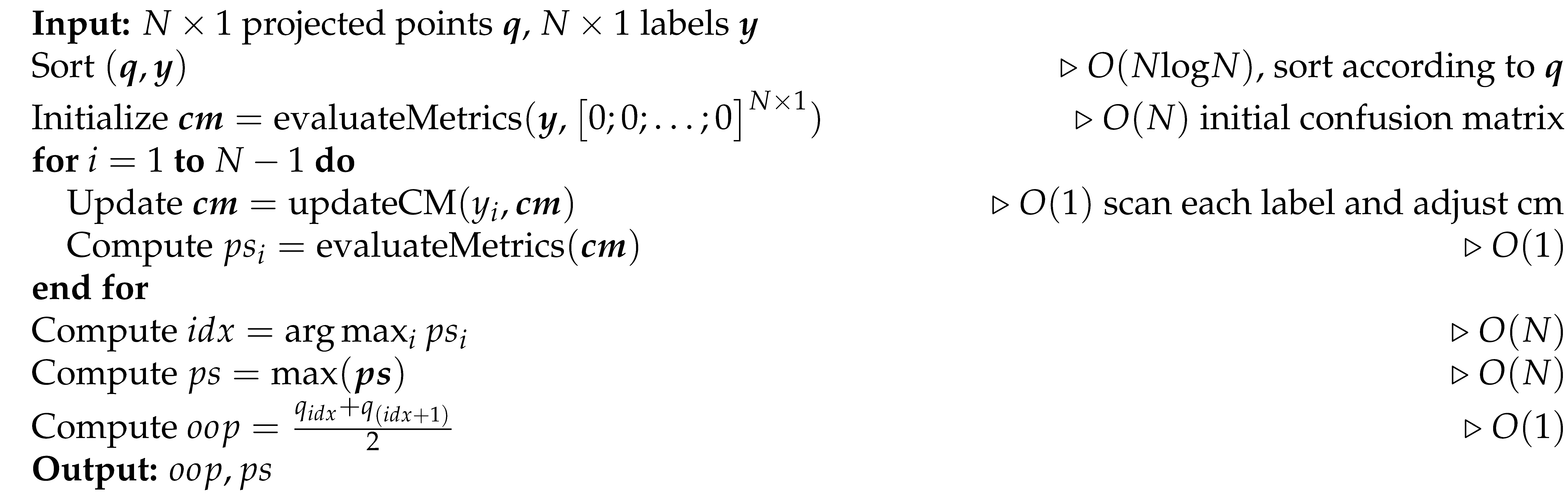
To classify data to different classes, a bias is required in addition to the classification discriminant to offer a decision boundary for data projected onto the discriminant. Given N samples, the data points are projected onto CDB and sorted, from which operating point (OP) candidates are taken as potential decision boundary of the line, defined as the middle point of any two consecutive sorted coordinate. Each OP candidate is associated with a performance-score, defined as (see Appendix E for the formula), where pos and neg means evaluating metric for each class. The performance score is a comprehensive metric that simultaneously considers sensitivity, recall, and specificity, providing a fair evaluation for biased models on imbalanced datasets, owing to the more conservative AC-score metric Wu and Cannistraci (2025). An all-negative prediction as an initialization is compared with true labels to obtain the binary confusion matrix, which is then updated by scanning predicted labels one by one along CDB. The OP candidate with the maximum performance-score is selected as the OOP of the classifier. With this OOP search strategy, any vector in the space of CDB can be associated with a performance-score. Alg. 3 shows the pseudocode for the OOP search whose time complexity is .
3.2. CDA as Consecutive Geometric Rotations of CDB in 2D Planes
From the function optimization perspective, binary classification problems can be regard as maximizing certain performance metrics in multi-dimensional space. However, it is impractical to explicitly find the global optimum. Instead, a feasible technique is to find a path that gradually approaches the region close to the global optimum or suboptimum, escapes from local minimum as much as possible.
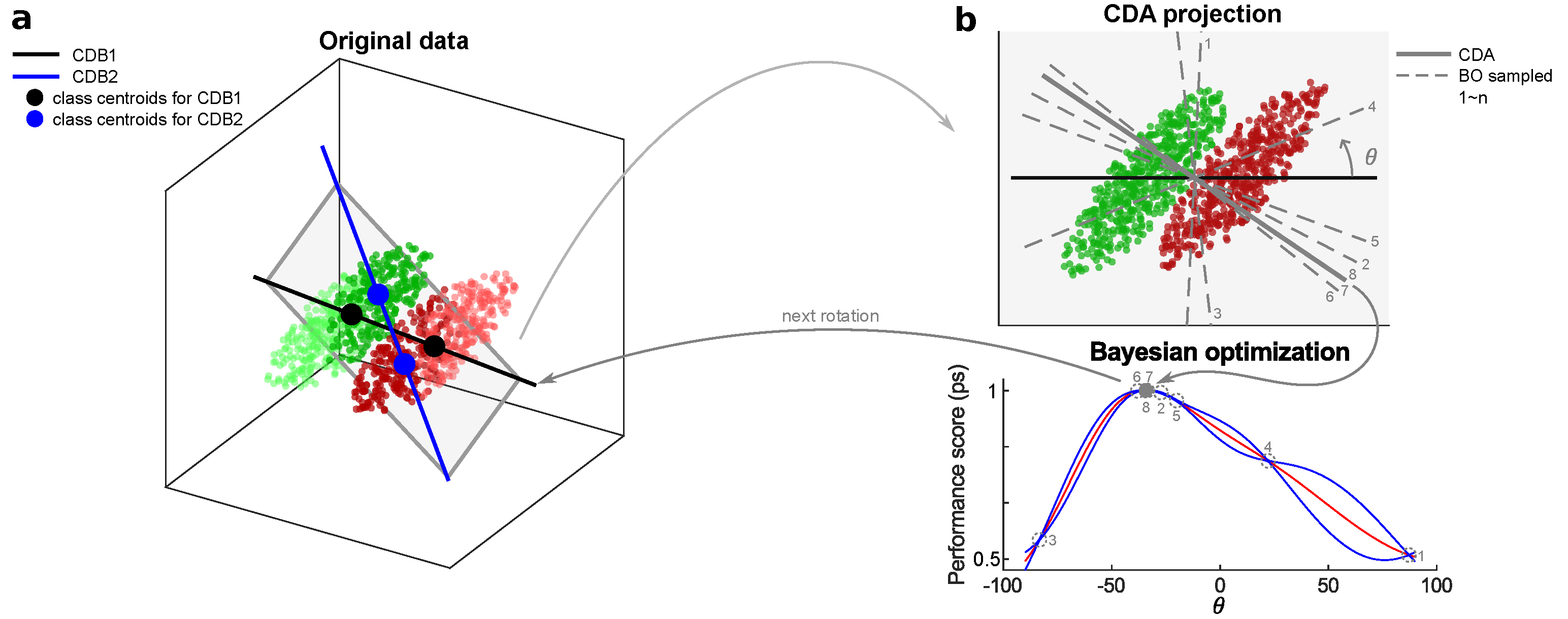
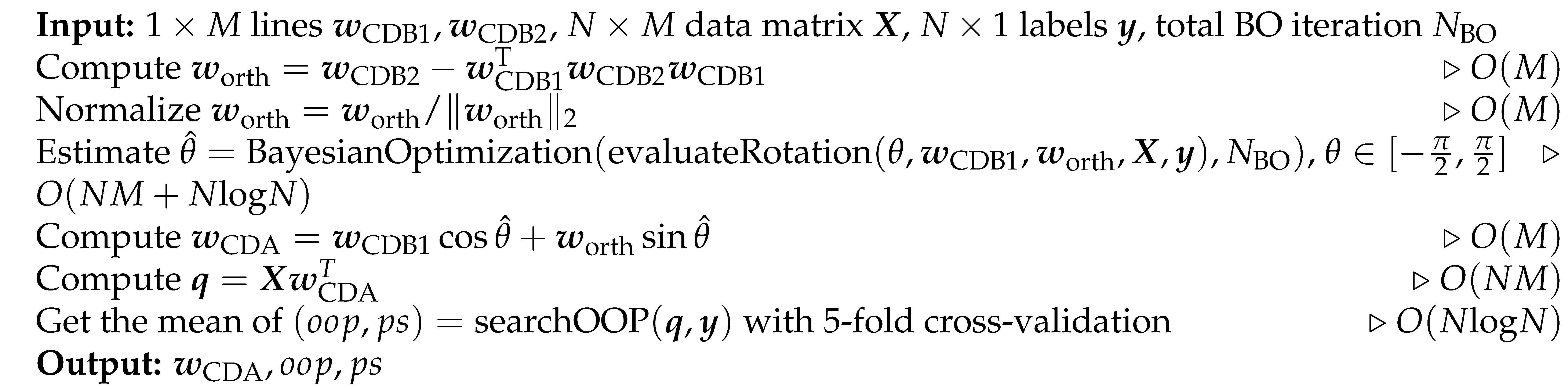
Based on the above problem formulation, our idea is to start the optimization path from CDB0, continuously rotate the classification discriminant in 2D planes in which there is a high probability of having a better performance classification discriminant. To construct such a 2D plane with another vector, we observe that the samples falling in the region of the geometric space close to the decision boundary (i.e. OOP) should have more weights, because this region is prone to overlapping by samples from different classes, causing misclassification. Thus, we compute another CDB using centroids with shifted sample weights toward OOP. On the plane formed by these two CDBs, the best rotation is found by Bayesian optimization (see next subsection). For clarity, we have the following definition: the first vector in each rotation is termed as CDB1, the second vector in each rotation is termed as CDB2, the CDB searched with the best performance is termed as CDA, and at the end of each rotation CDA becomes CDB1 for the next rotation. CDA rotation is used to refer to this rotation process. Figure 1a shows the diagram for one of CDA rotations.
Figure 1.
CDA rotation diagram. (a) CDB1 is obtained from specific sample weights. CDB2 is obtained from centroids with a shifted sample weights toward the decision boundary. Darker points represent larger sample weights. CDB1 and CDB2 form a plane on which BO is performed to estimate the best classification discriminant. (b) The progress of BO to estimate the best discriminant. The rotation angle from CDB1 is the independent variable to search in BO. CDB: Centroid Discriminant Basis; CDA: Centroid Discriminant Analysis
The sample weights shift mechanism is described as follows. Given CDB1 and its OOP in each CDA rotation, the distance of all projections to OOP can be obtained by , which is then reversed by , in align with the purpose that points close to decision boundary have larger weights. Since only the relative information of sample weights is important, they are L2-normalized and decayed smoothly from previous sample weights by , where ⊙ indicates the Hadamard (or element-wise) product. Specifically, in the first CDA rotation, the CDB1 is obtained with uniform sample weights, which corresponds to CDB0 in the GDA theory.
The CDA training stops when meeting any of the two criteria: (1) Reach the maximum 50 iterations. (2) the coefficient of variance (CV) of the last 10 performance-score is less than a threshold (set as 0.001 in the experiments) which means that the training has converged. Alg. 1,2 and 4 show the corresponding pseudocode.
3.3. Bayesian Optimization
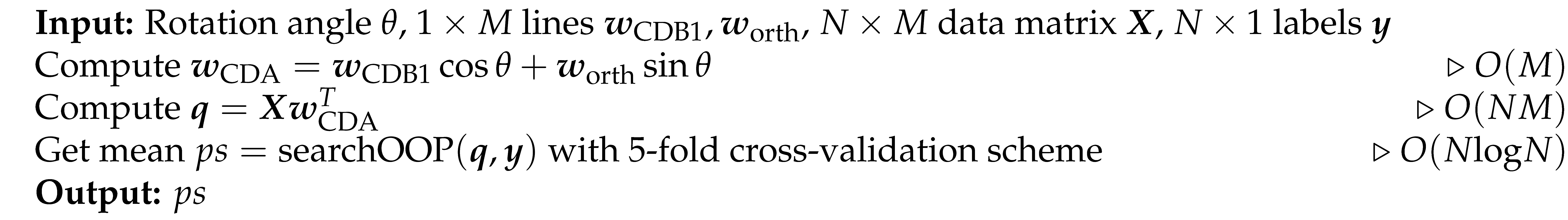
The CDA rotation aims to search for a unit vector CDB with the best performance-score, which can be efficiently realized by BO. BO Frazier (2018) is a statistical-based technique to estimate the global minimum of a function with as fewer evaluations as possible, and more sampling leads to more accurate estimation of global minimum. CDA leverages this high-efficiency characteristic of BO to achieve a fast training. BO itself has the time complexity of when it searches a single parameter, where Z is the number of sampling-and-evaluations. In CDA, the number of BO sampling is bounded to Z=10 for CDA rotation, which is a small constant.
Another factor to the effectiveness of CDA is the estimation with varying precision in BO. We set the number of BO sampling times to as default parameter during the CDA rotation, where is the -th rotation. During the first few CDA rotations, the BO estimation has relatively less precision. This gives CDA enough randomness to first enter a large region in which there are more discriminants with high performance, under the hypothesis that regions close to global optimum or suboptimum have more high-performance solutions that are more likely to be randomly selected. Starting from this large region, BO precision is gradually enhanced to refine the search in or close to this region in terms of Euclidean distance, and force CDA to converge. The upper limit of 10 CDA rotations still creates a small level of imprecision, in order to make CDA escape from small-size local minimum, to acquire higher performance, and improve training efficiency. Figure 1b shows an instance of BO working process. Alg. 5 shows the pseudocode for the CDA rotation as the black box function to optimize by BO.
3.4. Refining CDA with Statistical Examination on 2D Plane
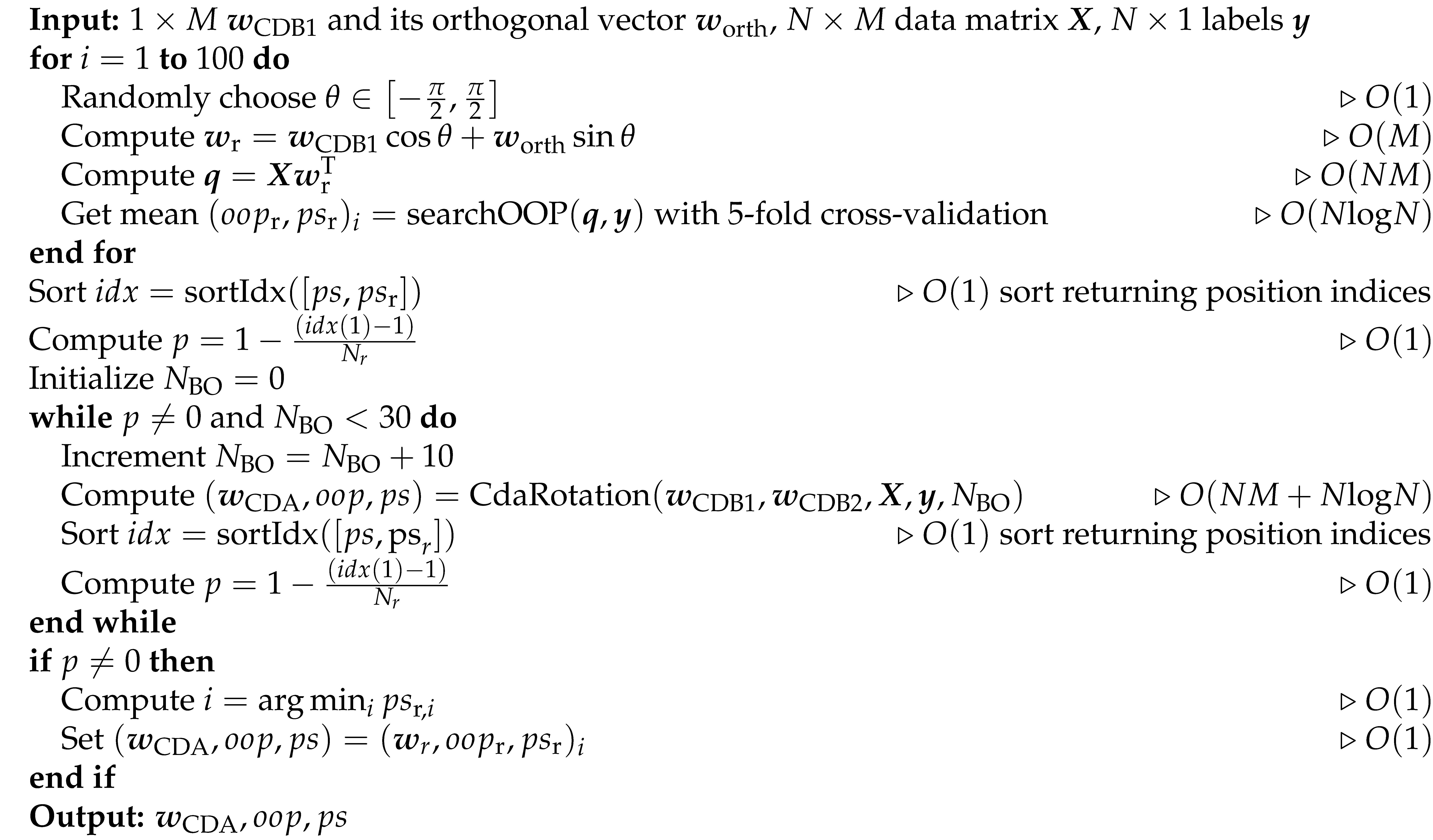
In CDA, the plane associated with the best performance is selected, but it is uncertain whether there are higher-performance discriminants on this plane, since the precision might not be high enough with 10 BO samplings and even lower for less samplings. To determine whether the BO is precise enough, a statistical examination using p-value with respect to null-model is performed. On this best plane, we generate 100 random CDBs, run BO in turn for 10, 20 and to the maximum 30 BO samplings, until the p-value of training performance-score of the BO-estimated CDB with regard to the null model is 0, otherwise using the best random CDB. In this way, we are able to give a confidence level of the BO estimated discriminant in the best CDA rotation plane. Alg. 6 shows the pseudocode for the refining finalization step.
3.5. Extend CDA for Multiclass Prediction via ECOC
Error-correcting output codes (ECOC) Allwein et al. (2001) is a method to make multiclass predictions from trained binary classifiers. To predict the class labels of a sample, multiple scores can be obtained on the set of trained binary classifiers. These scores are interpreted as they are either for or against a particular class. Depending on the coding matrix and the loss function chosen, ECOC takes the class with the highest overall reward or lowest overall penalty as the predicted class. In this study, the coding matrix for one-versus-one training scheme is selected, as it creates more linearly separability Acevedo et al. (2022); Aldo and Wu (2024). For the type of loss function, hinge-loss is chosen, as our internal tests suggested this loss leads to the best classification performance for each tested linear classifier.
4. Experimental Evidences on Real Data
In this section, we compared the proposed CDA classifier with other linear classifiers. The selected linear classifiers include LDA, SVM and fast SVM, which are widely recognized as state-of-the-art, first-to-try linear classifiers for binary classification tasks. Additionally, we include the baseline method, CDB0 (which is equivalent to NMC with OOP bias), to quantify the improvements made by CDA over a simplistic centroid-based classification approach.
4.1. Algorithm Scalability
To evaluate scalability, we used a metric called empirical time complexity Wu and Cannistraci (2025) (ETC), which is a data-driven model-free and parameter-free method to account for the factors influencing an algorithm; for instance, the crosstalk between algorithm realization, compilation and hardware implementation. ETC normalizes runtimes and input sizes relative to their smallest values ( and ) as and respectively. By taking the logarithms of these normalized variables, the resulting curve visually represents how the algorithm scales with input size, highlighting the practical challenges of scaling in real-world applications.
The scalability tests used the CIFAR10 dataset Krizhevsky (2009). Images were flattened into a 1D representation, constructing a data matrix where each row corresponded to one image. The input matrix size was controlled by trimming it to square matrices with widths of 4096, 8192, and 16384. Overhead time unrelated to data size was deducted from training times (training times without overhead deduction is in Figure 7). For each data size, experiments were repeated five times using random sampling (with replacement) of features and samples, and ETC was calculated for each iteration.
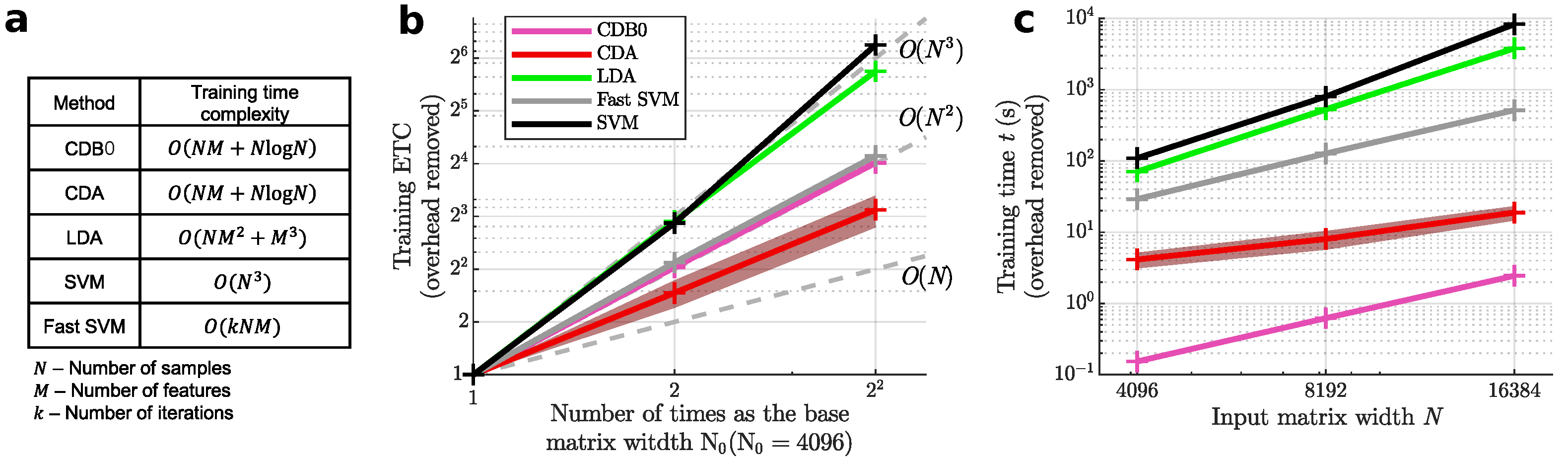
Figure 2a shows the theoretical time complexities of the tested linear methods, while Figure 2b presents their ETC results. CDA demonstrated the lowest time complexity, falling between linear and quadratic scales. SVM exhibited the highest time complexity, followed by LDA. Fast SVM achieved slightly worse scalability than quadratic time, while the baseline method CDB0 aligned with quadratic scaling. In Figure 2c, CDA also achieved a low absolute runtime only slower than the baseline CDB0 approach. In terms of absolute runtime (Figure 2c), CDA was second only to CDB0. These results highlight CDA’s efficiency, offering fast training times for smaller datasets and superior scalability for very large datasets.
Figure 2.
(a) Theoretical training time complexity of linear classifiers. (b) Empirical time complexity (ETC) shows how each linear method scales in training time as input matrix size increases in (c). Grey lines are references of cubic, square and linear functions. The number of features were set the same as number of samples N. (c) The training time of linear classifiers with increasing input matrix sizes. Log-scale is used for both axes to reveal the scalability of algorithms in (b) and (c). Shaded area represents standard error. CDB0: Centroid Discriminant Basis 0; CDA: Centroid Discriminant Analysis; LDA: Linear Discriminant Analysis; SVM: Support Vector Machine
4.2. Classification Performance on Real Data
We assessed classification performance across 27 datasets, including standard image classification Coates et al. (2011); Cohen et al. (2017); Hull (1994); Krizhevsky (2009); LeCun et al. (1998); Netzer and Wang (2011); Nilsback and Zisserman (2008); Stallkamp et al. (2011); Xiao et al. (2017), medical image classification Yang et al. (2023), and chemical property prediction tasks Wu et al. (2018). These datasets represent a broad range of real-world applications and varying data sizes, enabling an evaluation of both training speed and predictive performance. Each dataset was split into a 4:1 ratio for train-validation and test sets. The train-validation set was further divided into a 4:1 ratio for five-fold cross-validation. The final model for each method was an unweighted ensemble of the five cross-validated models.
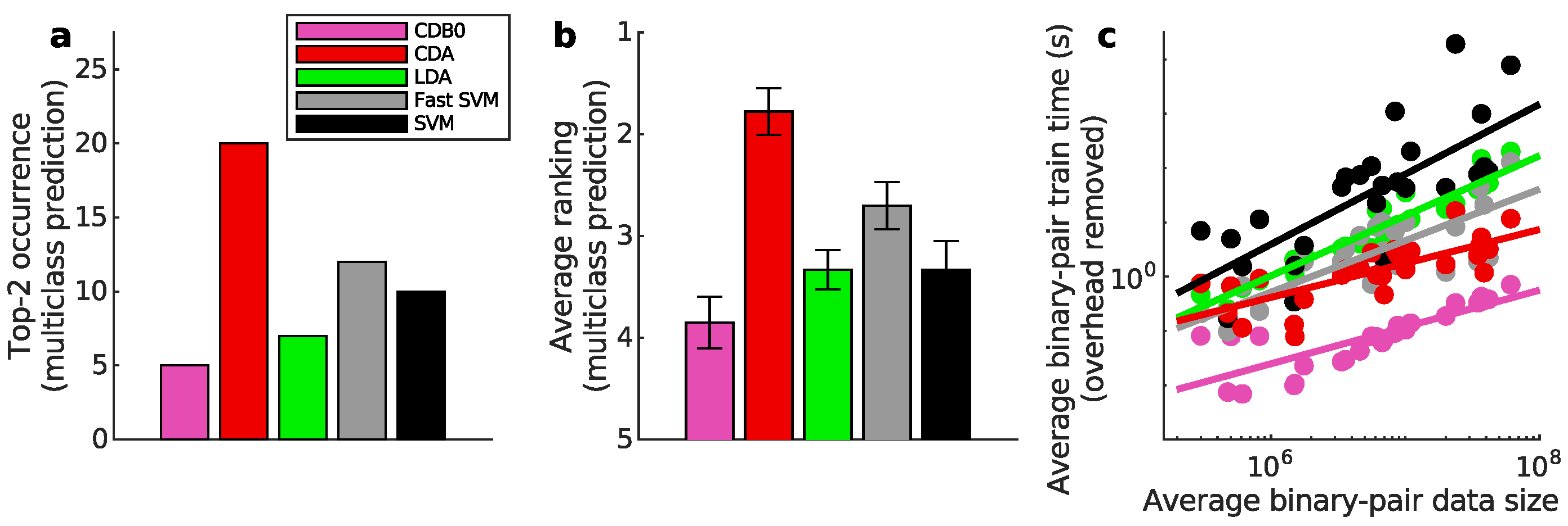
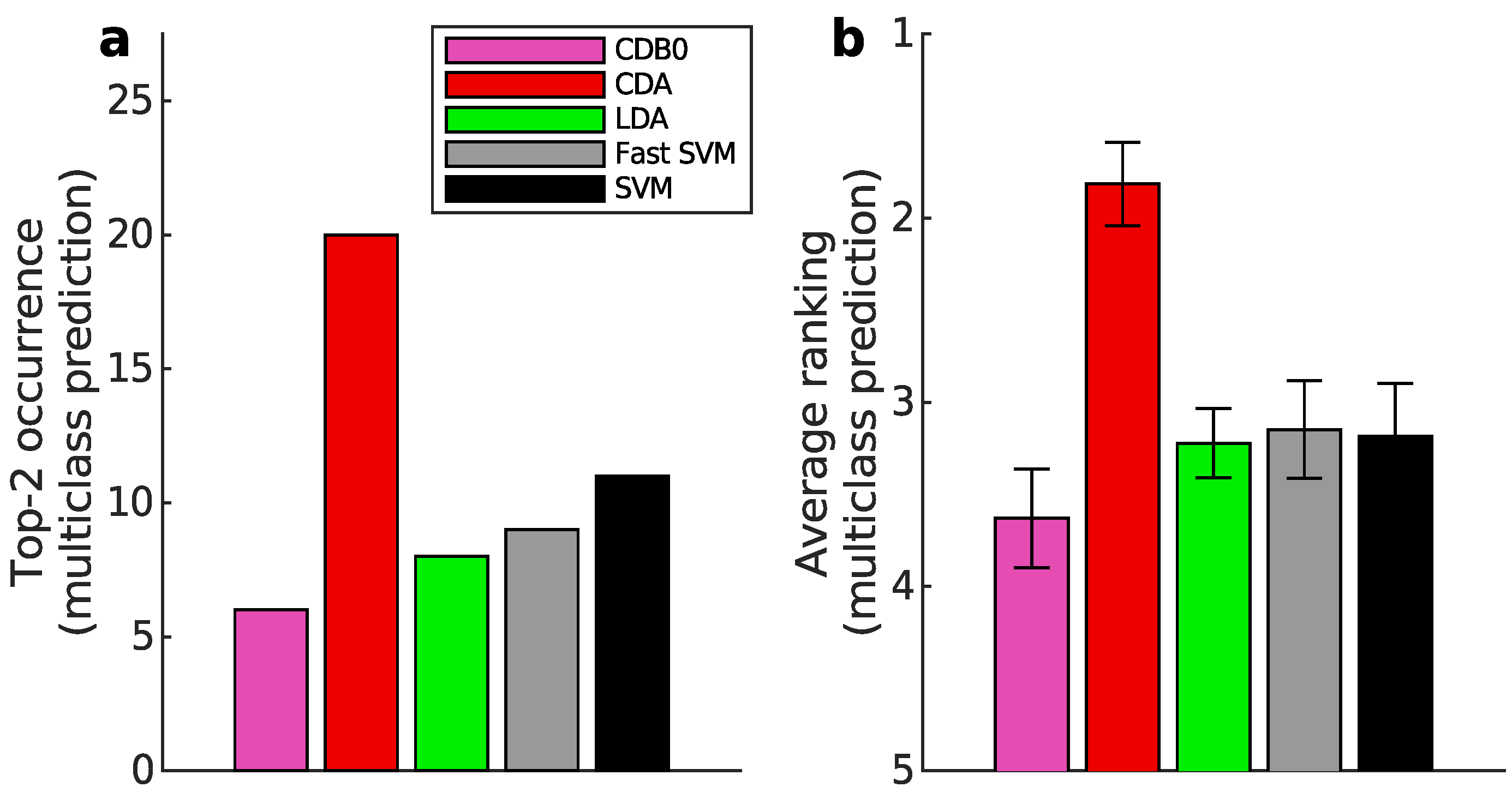
Figure 3a-b present the multiclass prediction performance on the test sets. In Figure 3a, CDA achieved a top-2 occurrence in 20 out of 27 datasets based on AUROC, indicating its stability and competitiveness. Figure 3b shows that CDA achieved the highest average ranking which is 1.78, outperforming LDA and SVM, with statistically significant margins as indicated by standard error bars. See Appendix I-J for binary classification results, ranking results based on AUPR, F-score, and accuracy, and the complete performance table.
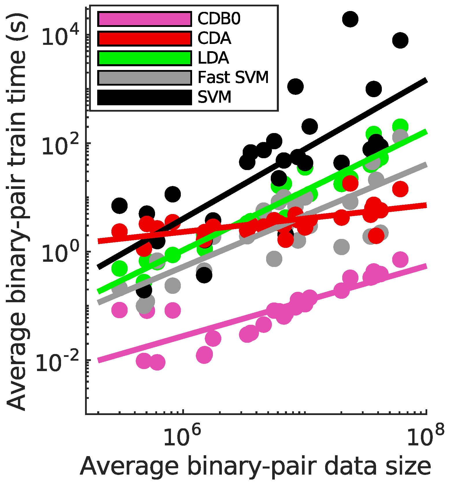
Figure 3c compares training speeds across datasets. Train times per binary-pair were averaged after deducting constant overheads unrelated to data size (The time without overhead deduction is in Figure 8). A logarithmic regression of train times and data sizes shows that CDA and CDB0 exhibit the best scalability, followed by fast SVM, LDA, and SVM, consistent with their theoretical complexities. CDA not only improves significantly over CDB0 in performance but also retains similar scalability. This improvement is driven by three key components: generalized centroids with non-uniform weights, sample weight shifts, and BO. The weighted average number of iterations required by CDA per dataset was 29.33 - a small constant that does not contribute to time complexity. By comparison, fast SVM’s iterations increase significantly with more challenging datasets. Considering the diversity of tested datasets, CDA demonstrates itself as a generic classifier with strong performance and scalability, making it applicable to large-scale classification tasks across varied domains.
Figure 3.
Classification performance on 27 real datasets. (a) Top-2 occurrences of algorithms according to AUROC in multiclass prediction tasks, highlighting their prevalence in high-performing outcomes. CDA shows the highest frequency of top-2 occurrences, followed by other algorithms. (b) Average ranking of algorithms according to AUROC in multiclass prediction tasks. CDA consistently ranks highest, indicating strong performance. Error bars represent standard errors. (c) Relationship between average binary-pair training time and average binary-pair data size. Log-scale is used for both axes to reveal the scalability of algorithms. Linear regression is applied to the logarithms of average binary-pair training time and that of average binary-pair data size. CDB0: Centroid Discriminant Basis 0; CDA: Centroid Discriminant Analysis; LDA: Linear Discriminant Analysis; SVM: Support Vector Machine
4.3. Interpretation on the Experiment Results
Unlike traditional classification methods, CDA employs performance-dependent training, directly optimizing task-specific metrics. While other classifiers can also be framed as optimization problems (for instance, neural networks minimizing entropy loss, LDA minimizing variance ratios, and SVM minimizing margins with misclassification penalties), incorporating a metric evaluation term often compromises their foundational principles or complicates the optimization process. For instance, it could render derivative-based solutions infeasible in neural networks and SVM, or disrupt covariance matrix inversion in LDA.
For large-scale datasets, CDA shows clear advantages. When , SVM has a speed advantage, though the curse of dimensionality often arises in this regime. When , LDA can train faster but has reduced effectiveness to outliers and highly correlated features. CDA and fast SVM strike a balance between samples and features, achieving lower time complexity. Moreover, CDA’s iterations remain stable regardless of dataset difficulty, making it particularly suitable for square-like datasets with comparable sample and feature counts. In such cases, CDA maximizes its speed advantage over LDA, fast SVM, and SVM while mitigating overfitting.
5. Case Study: In Which Cases Does CDA Overcome ResNet?
We know that ResNet He et al. (2016) is the state-of-the-art for image classification. However, in this section we use a case study to explain the condition in which using CDA is more convenient than using more elaborated methods such as ResNet. Specifically, we compare CDA with ResNet on the adrenal dataset from MedMNIST Yang et al. (2023), which contains 3D shape information from abdominal CT images of human adrenals, labeled as either normal adrenal gland or adrenal mass disease. Each sample is a 28 × 28 × 28 binary 3D matrix, which is flattened into a 1D vector for CDA, while ResNet processes the data without transformation. As a widely used metric in the medical field, AUROC is chosen for evaluation as it captures both sensitivity and false-positive rates (see Appendix E).
Figure 4.
Test set AUROC of different models. CDA (red) achieves the highest AUROC, surpassing the ResNet18-2.5D model evaluated at both the best validation epoch (yellow) and the best training epoch (dark yellow). The results highlight CDA’s superior performance in this task. CDA: Centroid Discriminant Analysis.
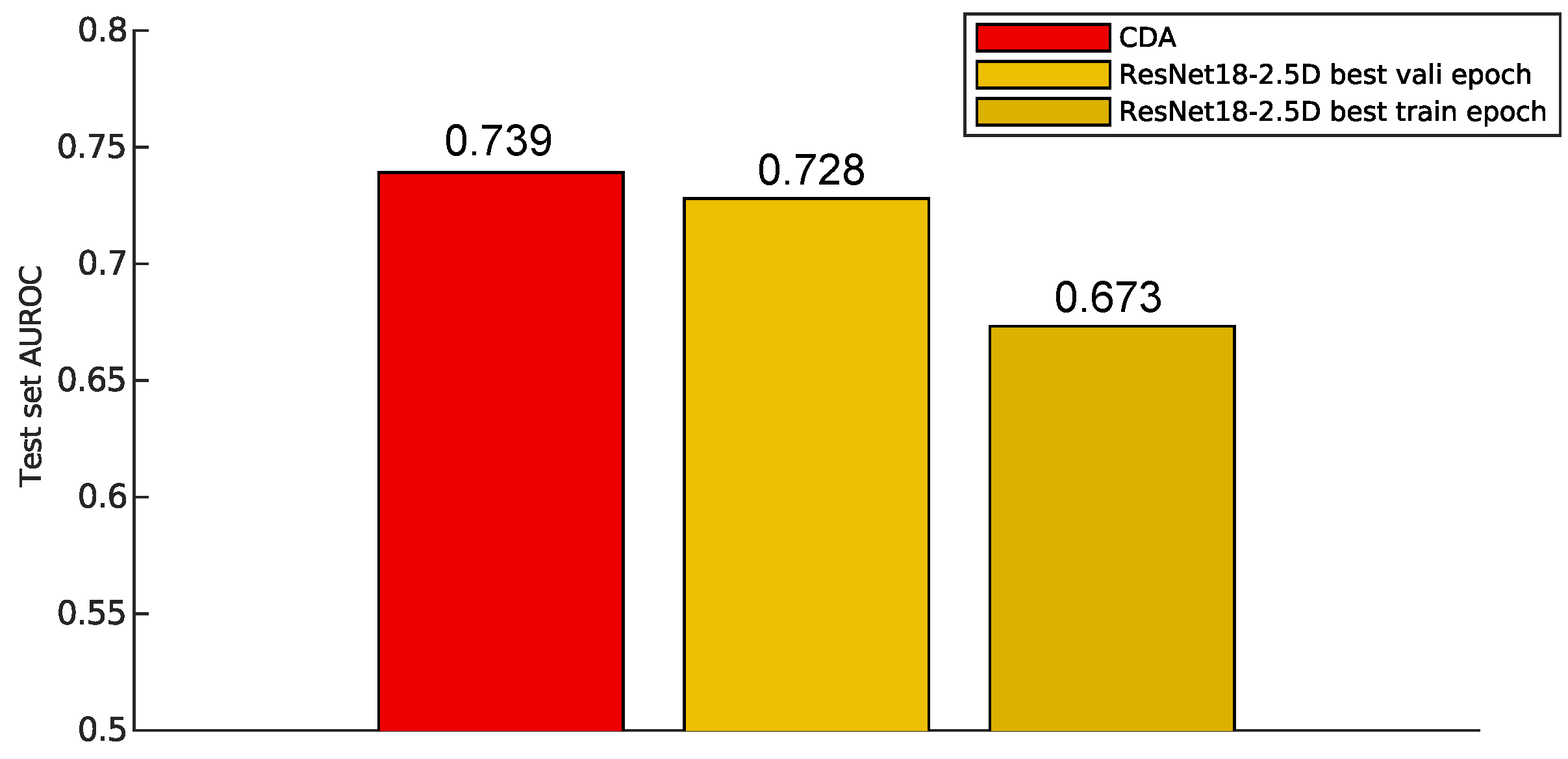
The ResNet model used for comparison is ResNet18-2.5D, which performs channel-wise convolutions but does not apply convolutions across the third channel representing CT slices. The model was trained for 100 epochs, and predictions were made using two versions: one from the epoch with the best training performance and another from the epoch with the best validation performance. The test on the best training model ensures a direct comparison with CDA, which does not incorporate a validation-based selection mechanism.
As shown in Figure 4, CDA not only outperformed the ResNet model trained for optimal training performance but also surpassed the model selected based on validation performance in terms of AUROC. Since validation-based model selection is a common technique for mitigating overfitting, this suggests that CDA inherently resists overfitting.
While ResNet is highly effective for complex tasks, CDA proves to be a better choice for problems where classification does not rely heavily on nonlinear relationships between input data and labels. Compared to neural network-based approaches like ResNet, CDA offers significantly reduced overfitting tendencies and much more efficient training, even when overfitting mitigation techniques are applied in ResNet. This finding is consistent with prior research indicating that biomedical imaging data, such as MRI brain scans, often exhibit low nonlinearity, making simple linear methods as effective as nonlinear approaches Schulz et al. (2020).
6. Conclusions and Discussions
The development of supervised classification techniques often encounters a trade-off between scalability and predictive performance. Linear classifiers, while inherently simpler, are favored in certain contexts due to their reduced tendency to overfit and their interpretability in decision-making. However, achieving both high scalability and robust predictive performance simultaneously remains a significant challenge.
In this study, the introduction of the Geometric Discriminant Analysis (GDA) framework marks a notable step forward in addressing this challenge. By leveraging the geometric properties of centroids – a fundamental concept in multiple disciplines – GDA provides a unifying framework for certain linear classifiers. The core innovation lies in the Centroid Discriminant Basis (CDB), which serves as the foundation for deriving discriminants. These discriminants, when augmented with geometric corrections under varying constraints, extend the theoretical flexibility of GDA. Notably, Nearest Mean Classifier (NMC) and Linear Discriminant Analysis (LDA) are shown to be a subset of this broader framework, demonstrating how they converge to CDB under specific conditions. This theoretical generalization not only validates the GDA framework but also sets the stage for novel classifier designs.
A key practical contribution of this work is the Centroid Discriminant Analysis (CDA), a specialized implementation of GDA. CDA employs geometric rotations of the CDB within planes defined by centroid-vectors with shifted sample weights. These rotations, combined with Bayesian optimization techniques, enhance the method’s scalability, achieving quadratic time complexity . This performance represents a substantial improvement over traditional linear methods such as LDA, Support Vector Machines (SVM), and fast SVM.
The experimental results further highlight CDA’s advantages. Across diverse datasets—including standard images, medical images, and chemical property classifications—CDA demonstrated superior performance in scalability, predictive accuracy, and stability. Particularly noteworthy is its competitive performance against state-of-the-art methods like ResNet in tasks such as medical image classification, where CDA exhibited reduced overfitting tendencies. This result underscores the potential of geometric approaches in bridging the gap between linear methods and deep learning models, particularly in scenarios demanding both interpretability and efficiency. CDA has a significantly less training time and prediction time compared to nonlinear methods. CDA is especially powerful for large square data matrix, e.g. the number of samples is close to features, because in such condition the samples are enough to reduce overfitting, and CDA increases the speed advantage over LDA and SVM.
These findings not only validate the efficacy of the proposed CDA method but also open avenues for further exploration. The GDA framework’s flexibility invites the development of additional classifiers tailored to specific application needs, leveraging the geometric principles underpinning CDB. Future research may focus on extending this framework to non-linear discriminants or exploring its integration with deep learning architectures to further enhance performance while maintaining scalability and gaining efficiency.
In conclusion, the GDA framework and its CDA implementation represent a paradigm shift in classifier design, combining the interpretability of geometric principles with state-of-the-art computational efficiency. This work not only advances the field of linear classification but also lays groundwork for innovative approaches to supervised learning.
Impact Statement
This paper presents work whose goal is to advance the field of Machine Learning. There are many potential societal consequences of our work, none which we feel must be specifically highlighted here.
A. GDA Demonstration with 2D Artificial Data
Figure 5.
(a) A 2-dimensional instance showing that LD (blue dashed) can be constructed from CDB0 (black solid) using covariance correction which is a geometrical correction. (b) The evolution from CDB0 to LD. The first equation is the general form of geometrical discriminants (GD) that can be constructed by CDB0 with its geometric corrections. If only one correction exists and this correction is a covariance-related matrix, LD can be derived from the general expression. CDB0: Centroid Discriminant Basis 0; LD: Linear Discriminant
Figure 6.
The GDA theory in 2 dimensions showing how the relation between LD and CDB0 evolves under specific conditions. (a) The relation between LD and CDB0 proceeds from the general case to different special case under the condition shown along each arrow. (b) The specific expressions of LD in terms of CDB0 and its corrections corresponding to each case in column (a). (c) Binary classifications results of LD (blue dashed) and CDB0 (black solid) on different 2D data corresponding to each case in column (a). LD: Linear Discriminant; CDB0: Centroid Discriminant Basis 0.
B. Pseudocode
This study deals with a supervised binary classification problem on labeled data with N samples and M features. The samples consist of positive and negative class data and with sizes and , respectively, and the corresponding labels are tokenized as 1 and 0, respectively. The sample features are flattened to 1D if they have higher dimensions, such as image data. The following section introduces CDA in pseudo-code. CDA rotations, BO sampling and p-value computing involve constant numbers, thus, they do not contribute to the time complexity.
| Algorithm 1: CDA Main Algorithm (CDA) |
 |
| Algorithm 2: Update Sample Weights (updateSampleWeights) |
 |
| Algorithm 3: Search Optimal Operating Point (searchOOP) |
 |
| Algorithm 4: Approximate Optimal Line by BO (CdaRotation) |
 |
| Algorithm 5: Evaluate the Line with Rotation Angle (evaluateRotation) |
 |
| Algorithm 6: Refine on the Best Model (refineOnBestPlane) |
 |
C. Deriving LDA in the GDA Theory for m-Dimensions (m>2)
In the GDA theory, we have demonstrated that linear discriminant (LD) can be expressed by the basis CDB0 with different geometric corrections on CDB0 under different conditions, as shown in Figure 6. The conclusions are not confined only to the 2-dimensional case but also applicable to the m-dimensional case (). Here we derive the generalization of the LD coefficient to the m-dimensional case. The discriminant of LDA is given by , where it is assumed that the within-class covariance matrix is invertible, and is the sum of covariance matrices of individual classes. Denote the elements in , , and by , , and for all , respectively.
Special Case 1. Assume that pairwise features have the same covariance , and all pairwise features have the same covariance (In experiments, we relax the conditions to have similar variance and similar covariance). Then, , where is the identity matrix, and is the all-one matrix. According to the Woodbury matrix identity, we have , where is the matrix with all ones except on the diagonal. Thus, , which corresponds to the row for special case 1 in Figure 6.
Special Case 1.1. Based on the assumptions made in Special Case 1, we further assume that the two covariance matrices are similar, i.e., , so that for all . We further have , where is the Pearson correlation coefficient (PCC) between features i and j. Based on the assumptions made in this special case, all pairwise PCCs are the same, i.e., for all . Thus, , which shows that the geometric correction part is related to feature correlations. Thus, , which corresponds to the row for special case 1.1 in Figure 6.
Special Case 1.1.1. Based on Special Case 1.1, assume further that all pairwise features have no correlations (i.e., ), then according to the equation, . Thus, , which corresponds to the row for special case 1.1.1 in Figure 6. By these derivations, we show how LDA converges to CDB0 under specific conditions of the data.
D. Deriving CDA in the GDA Theory
In this section, we give the mathematical demonstration of how CDA is formulated in the GDA theory. Since the correction matrix for LDA in Section 2 is a special case of a linear operator, we extend to a more general correction term deriving CDA in the GDA theory. The construction of the geometric discriminant can be realized by continuously rotating CDB0 in planes that satisfy several constraints, shown by:
where , in which is the identity operator. For a given dataset are fixed, thus it is simplified by:
which defines the linear operator that maps the line CDB1 to CDA in each CDA iteration and maps the sample weights to the updated sample weights.
The second equality holds because obtained at the end of each rotation is used as in the next rotation. The fifth equality shows that the final CDA line can be written in a form that only depends on variables of the first iteration. This is because, in the first CDA rotation, the initial sample weights are uniform, and CDB1 is the same as CDB0 of the GDA theory. Thus, from the sixth equality, are omitted. The last three equalities show that the final CDA discriminant is a subcase of the generalized GDA theory.
The operator can be decomposed as two sequential operators:
where is the linear operator that maps CDB1 to CDB2. is the linear operator that maps two vectors CDB1 and CDB2 to the BO-estimated discriminant on the plane spanned by CDB1 and CDB2, and updates samples weights.
The operator does the mapping through the following equation:
The operator does the mapping through the following equation:
Where the first two equations find the unit orthogonal vector to CDB1 by the Gram-Schmidt process. The orthogonalization process ensures an efficient search in the space of CDBs during the rotation. The last two equations estimate the optimal rotation angle using Bayesian optimization and the corresponding discriminant.
is the operator that outputs the performance score given a classification discriminant, which projects all data onto the discriminant and performs the OOP search to find the score.
E. Classification Performance Evaluation
The datasets used in this study span standard image classification, medical image classification, and chemical property classification, most of which involve multiclass data. To comprehensively assess classification performance across these diverse tasks, we employed four key metrics: AUROC, AUPR, F-score, and AC-score. Accuracy was excluded due to its limitations in reflecting true performance, especially on imbalanced data. Though data augmentation can make data balanced, it introduces uncertainty due to the augmentation strategy and the data quality.
Since we do not prioritize any specific class (as designing a dataset-specific metric is beyond this study’s scope), we perform two evaluations—one assuming each class as positive—and take the average. This approach applies to AUPR and F-score, whereas AUROC and AC-score, being symmetric about class labels, require only a single evaluation.
For multiclass prediction, a C-dimensional confusion matrix is obtained by comparing predicted labels with true labels. This is converted to C binary confusion matrices by each time taking one class as positive and all the others as negative, and the final evaluation is the average of evaluations on these individual confusion matrices.
To interpret this evaluation scheme, consider the MNIST dataset and the AUPR metric as an example. In binary classification, for the pair of digits "1" and "2", it calculates the sensitivity-recall for detecting "1" and the sensitivity-recall for detecting "2", then takes the average. For other pairs, the calculation follows the same pattern. In the multiclass scenario, it considers the sensitivity-recall for detecting "1" and the sensitivity-recall for detecting "not 1", then takes the average. The same approach applies to other pairs.
For a fair comparison with ResNet, AUROC is evaluated in the same manner as in CDA, using a single-point measurement of the area under the curve rather than a set of scores typically used in neural networks for binary classification.
Individual Metrics
(a) AUROC
Area Under the Receiver Operating Characteristic curve involves the true positive rate (TPR) and false positive rate (FPR) as follows:
This measure indicates how well the model distinguishes between classes. A high score means that the model can identify most positive cases with few false positives.
(b) AUPR
Area Under the Precision-Recall curve considers two complementary indices: precision () and recall (), defined as:
AUPR measures whether the classifier retrieves most positive cases.
(c) F-Score
F-score (using F1-score in this study) is the harmonic mean of precision and recall which contribute equally:
(d) AC-Score
An accuracy-related metric AC-score Wu and Cannistraci (2025) addresses the limitations of traditional accuracy for imbalanced data. It imposes a stronger penalty for deviations from optimal performance on imbalanced data and is defined as:
This metric assigns equal importance to both classes and penalizes imbalanced performance by ensuring that if one class is poorly classified, the overall score remains low. Thus, AC-score provides a more conservative but reliable evaluation of classifier performance.
(e) Performance-Score (ps)
The proposed CDA classifier employs performance-dependent learning, guided by a performance score (ps):
This formulation ensures a balanced consideration of both F-score and AC-score.
Though CDA as a generic classifier utilizes a relatively balanced metric, it can be customized to specific applications as needed.
F. Supplemental Training Speed Results
Figure 7.
The empirical time complexity (ETC) and training time with constant overhead kept. (a) ETC showing how each linear method scales with increasing input matrix sizes with respect to training time in (b). The grey lines are references with cubic, square and linear functions. The number of features were set the same as number of samples N. (b) The training time of linear classifiers with increasing input matrix sizes. Shaded area represents standard error. Log-scale is used for both axes to reveal the scalability of algorithms in (b) and (c). CDB0: Centroid Discriminant Basis 0; CDA: Centroid Discriminant Analysis; LDA: Linear Discriminant Analysis; SVM: Support Vector Machine
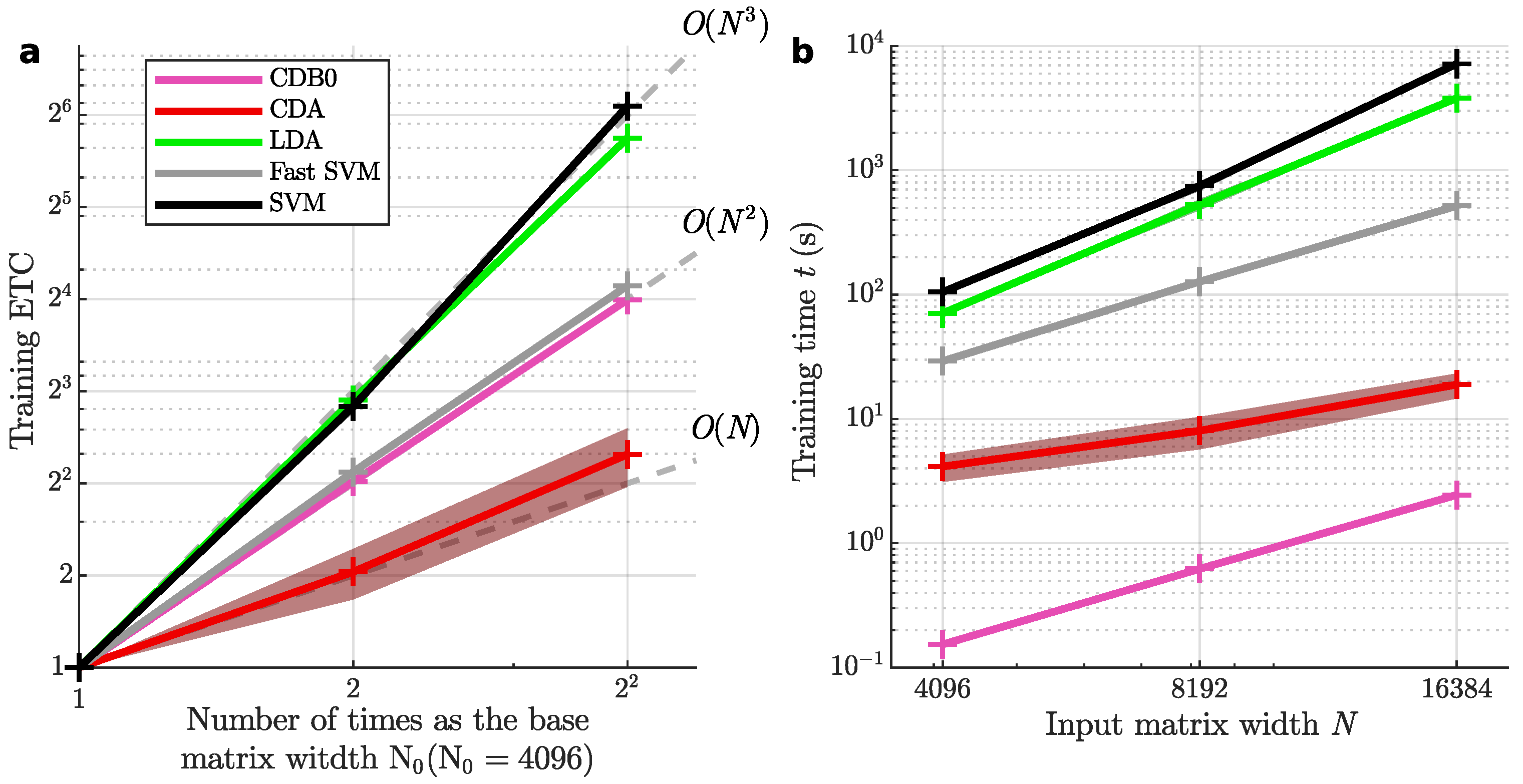
Figure 8.
Average binary-pair training time on 27 real datasets with constant overhead kept. Both axes are presented on a logarithmic scale to highlight the scalability of the algorithms. Linear regression is applied to the logarithms of average binary-pair training time and that of average binary-pair data size. CDB0: Centroid Discriminant Basis 0; CDA: Centroid Discriminant Analysis; LDA: Linear Discriminant Analysis; SVM: Support Vector Machine
G. Implementation Details of Linear Classifiers
Linear classifiers compared in this study include LDA, SVM, and fast SVM. Data were input to classifiers in their original values without standardization.
For LDA, the MATLAB toolbox function fitcdiscr was applied, with pseudolinear as the discriminant type, which solves the pseudo-inverse with SVD to adapt to poorly conditioned covariance matrices.
For SVM, the MATLAB toolbox function fitcsvm was applied, with sequential minimal optimization (SMO) as the optimizer. The cost function used the L2-regularized (margin) L1-loss (misclassification) form. The misclassification cost coefficient was set to by default. The maximum number of iterations was linked to the number of training samples in the binary pair as . The convergence criteria were set to the default values.
For fast SVM, the LIBLINEAR MATLAB mex function was applied. The cost function used the L2-regularized (margin) L1-loss (misclassification) form. The misclassification cost coefficient was set to by default. A bias term was added, and correspondingly, the data had an additional dimension with a value of 1. The convergence criteria were set to the default values. The maximum number of iterations was linked to the number of training samples in the binary pair as .
Hyperparameter tuning for LDA, SVM, and fast SVM was disabled, as the goal of this study was to compare linear classifiers fairly in a parameter-free condition. CDA, as well as CDB0, do not require parameter tuning.
Speed tests and performance test were from different computational conditions. To obtain classification performance in a reasonable time span, GPU was enabled for SVM, and multicore was. To compare speed fairly, all linear classifiers used single-core computing mode.
H. Dataset Description
The datasets tested in this study encompass standard image classification, medical image classification, and chemical property prediction, described in details in Table 1.

Table 1.
Dataset description
| Dataset | #Samples | #Features | #Classes | Balancedness | Modality/source | Classification task |
|---|---|---|---|---|---|---|
| Standard images | ||||||
| MNIST | 70000 | 400 | 10 | imbalanced | image | digits |
| USPS | 9298 | 256 | 10 | imbalanced | image | digits |
| EMNIST | 145600 | 784 | 26 | balanced | image | letters |
| CIFAR10 | 60000 | 3072 | 10 | balanced | image | objects |
| SVHN | 99289 | 3072 | 10 | imbalanced | image | house numbers |
| flower | 3670 | 1200 | 5 | imbalanced | image | flowers |
| GTSRB | 26635 | 1200 | 43 | imbalanced | image | traffic signs |
| STL10 | 13000 | 2352 | 10 | balanced | image | objects |
| FMNIST | 70000 | 784 | 10 | balanced | image | fashion objects |
| Medical images | ||||||
| dermamnist | 10015 | 2352 | 7 | imbalanced | dermatoscope | dermal diseases |
| pneumoniamnist | 5856 | 784 | 2 | imbalanced | chest X-Ray | pneumonia |
| retinamnist | 1600 | 2352 | 5 | imbalanced | fundus camera | diabetic retinopathy |
| breastmnist | 780 | 784 | 2 | imbalanced | breast ultrasound | breast diseases |
| bloodmnist | 17092 | 2352 | 8 | imbalanced | blood cell microscope | blood diseases |
| organamnist | 58830 | 784 | 11 | imbalanced | abdominal CT | human organs |
| organcmnist | 23583 | 784 | 11 | imbalanced | abdominal CT | human organs |
| organsmnist | 25211 | 784 | 11 | imbalanced | abdominal CT | human organs |
| organmnist3d | 1472 | 21952 | 11 | imbalanced | abdominal CT | human organs |
| nodulemnist3d | 1633 | 21952 | 2 | imbalanced | chest CT | nodule malignancy |
| fracturemnist3d | 1370 | 21952 | 3 | imbalanced | chest CT | fracture types |
| adrenalmnist3d | 1584 | 21952 | 2 | imbalanced | shape from abdominal CT | adrenal gland mass |
| vesselmnist3d | 1908 | 21952 | 2 | imbalanced | shape from brain MRA | aneurysm |
| synapsemnist3d | 1759 | 21952 | 2 | imbalanced | electron microscope | excitatory/inhibitory |
| Chemical formula | ||||||
| bace | 1513 | 198 | 2 | imbalanced | chemical formula | BACE1 enzyme |
| BBBP | 2050 | 400 | 2 | imbalanced | chemical formula | blood-brain barrier permeability |
| clintox | 1484 | 339 | 2 | imbalanced | chemical formula | clinical toxicity |
| HIV | 41127 | 575 | 2 | imbalanced | chemical formula | HIV drug activity |
I. Supplemental Performances on Real Datasets
I.1. Binary Classification
Figure 9.
Binary classification performance on 27 real datasets according to AUROC. (a) Top-2 occurrences of algorithms. (b) Average ranking of algorithms. Error bars represent standard errors. CDB0: Centroid Discriminant Basis 0; CDA: Centroid Discriminant Analysis; LDA: Linear Discriminant Analysis; SVM: Support Vector Machine.
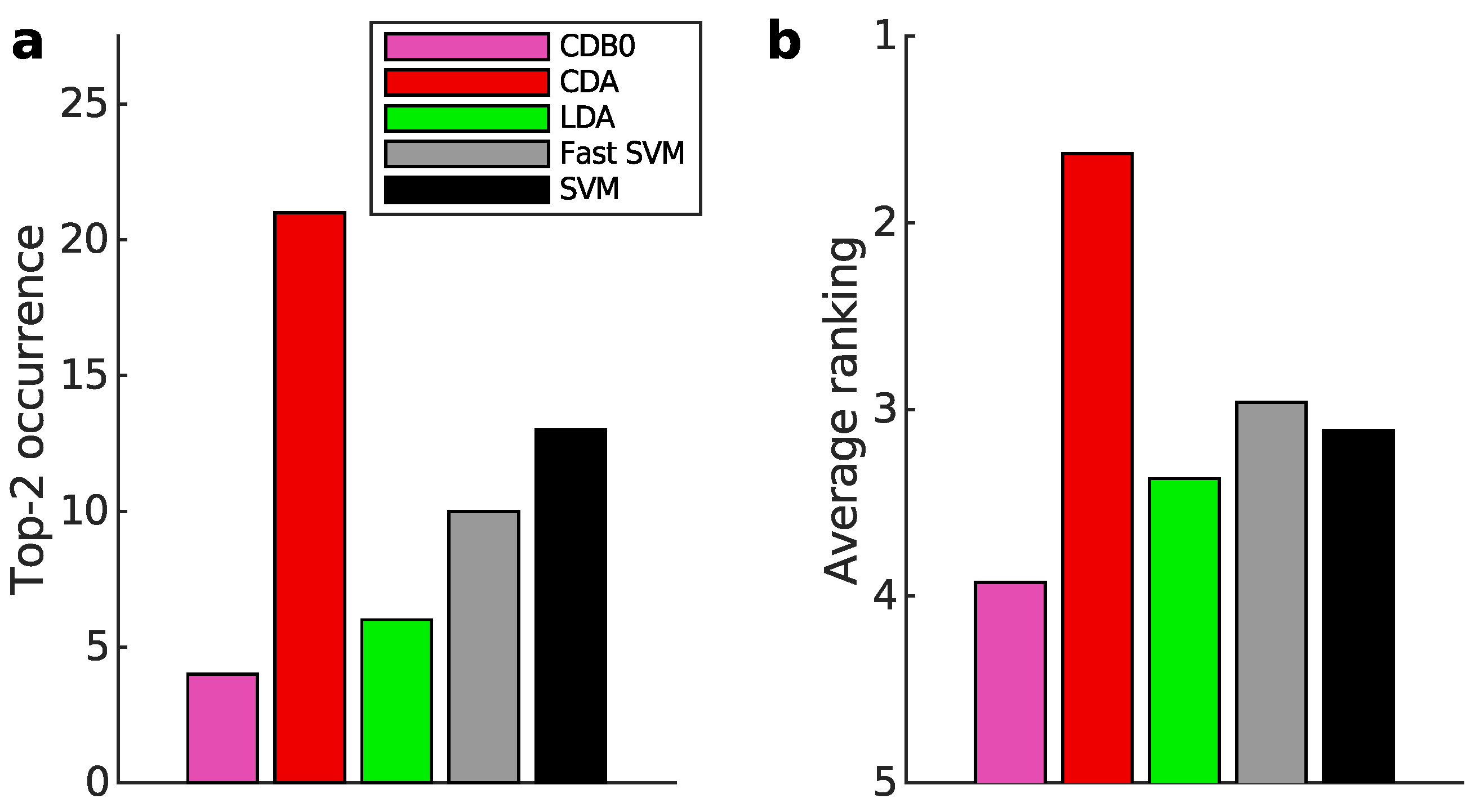
Figure 10.
Binary classification performance on 27 real datasets according to AUPR. (a) Top-2 occurrences of algorithms. (b) Average ranking of algorithms. Error bars represent standard errors. CDB0: Centroid Discriminant Basis 0; CDA: Centroid Discriminant Analysis; LDA: Linear Discriminant Analysis; SVM: Support Vector Machine.
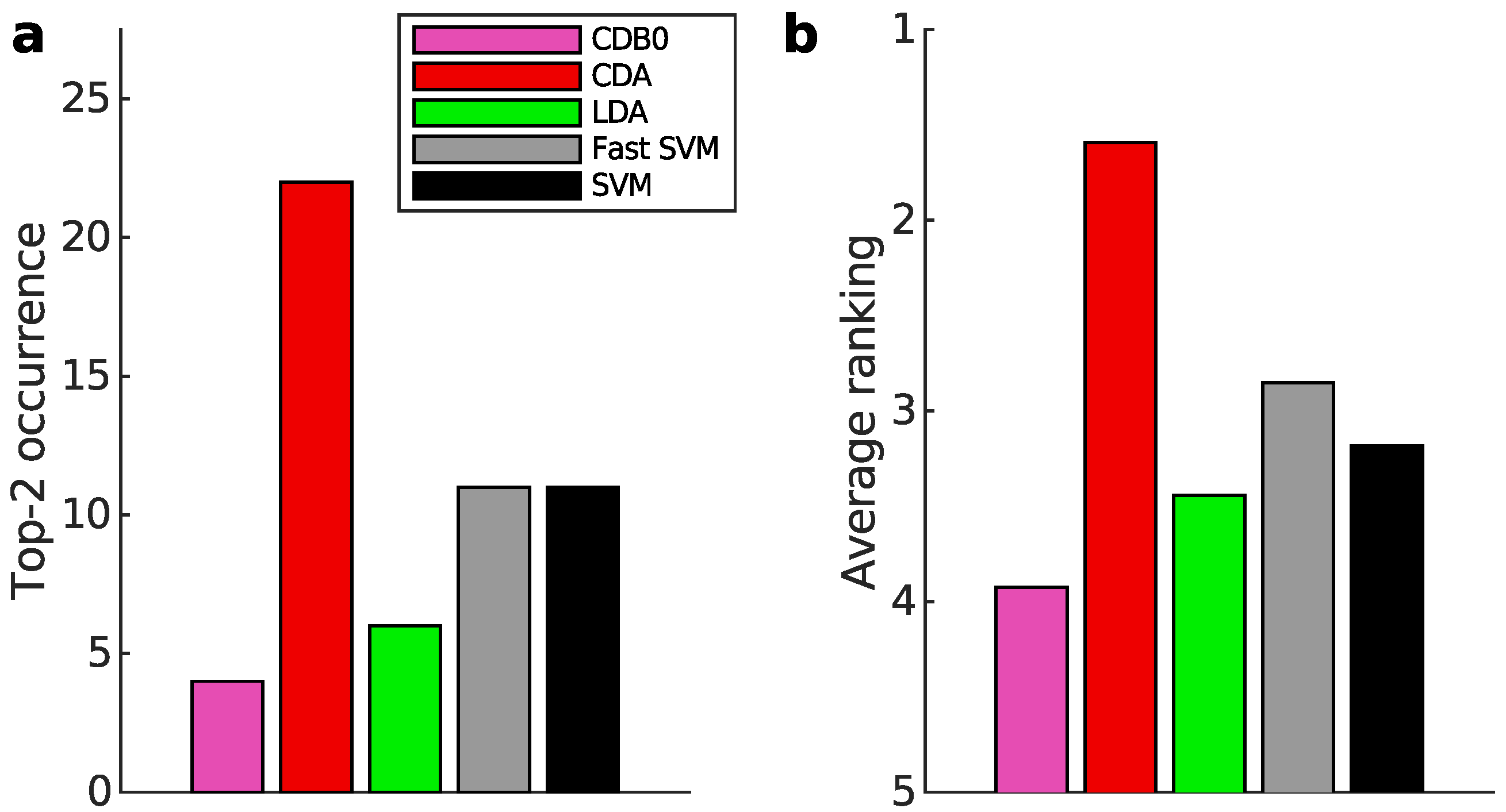
Figure 11.
Binary classification performance on 27 real datasets according to F-score. (a) Top-2 occurrences of algorithms. (b) Average ranking of algorithms. Error bars represent standard errors. CDB0: Centroid Discriminant Basis 0; CDA: Centroid Discriminant Analysis; LDA: Linear Discriminant Analysis; SVM: Support Vector Machine.
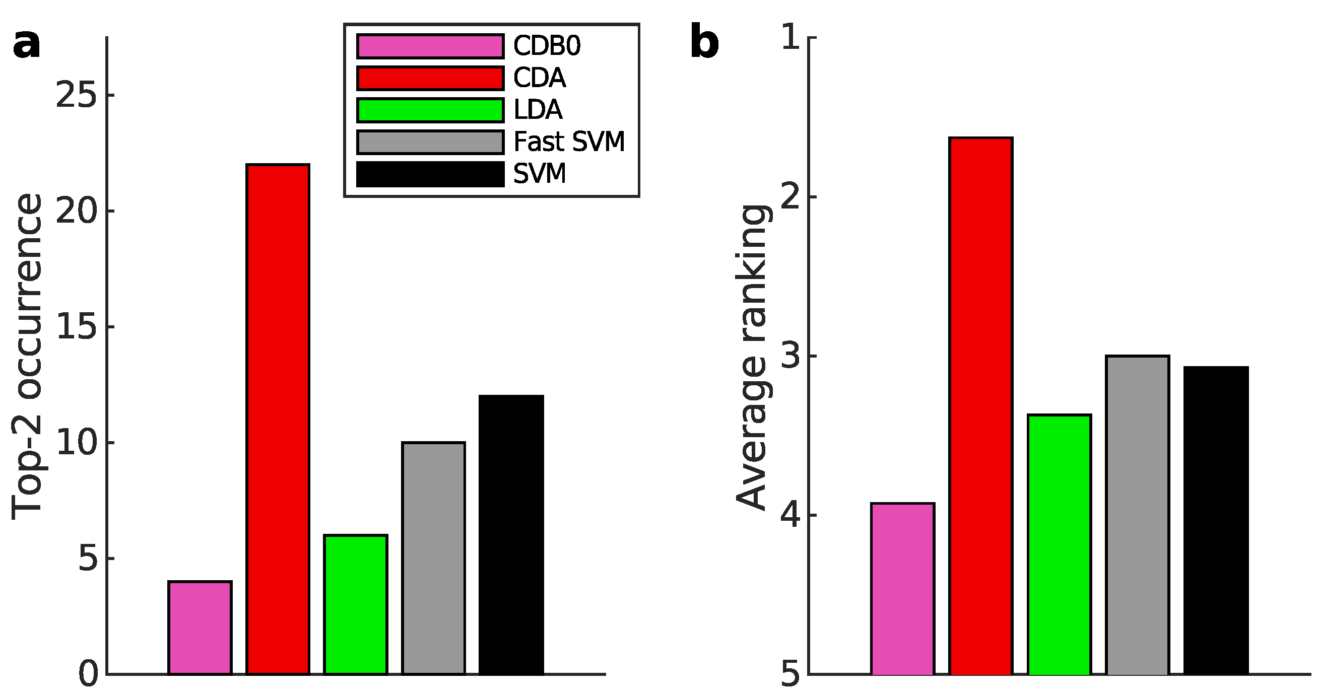
Figure 12.
Binary classification performance on 27 real datasets according to AC-score. (a) Top-2 occurrences of algorithms. (b) Average ranking of algorithms. Error bars represent standard errors. CDB0: Centroid Discriminant Basis 0; CDA: Centroid Discriminant Analysis; LDA: Linear Discriminant Analysis; SVM: Support Vector Machine.
I.2. Multiclass Prediction
Figure 13.
Multiclass prediction performance on 27 real datasets according to AUPR. (a) Top-2 occurrences of algorithms. (b) Average ranking of algorithms. Error bars represent standard errors. CDB0: Centroid Discriminant Basis 0; CDA: Centroid Discriminant Analysis; LDA: Linear Discriminant Analysis; SVM: Support Vector Machine.
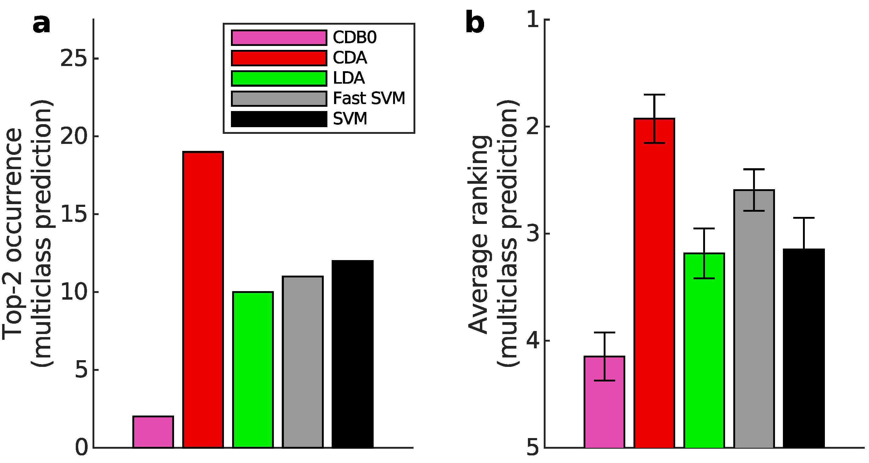
Figure 14.
Multiclass prediction performance on 27 real datasets according to F-score. (a) Top-2 occurrences of algorithms. (b) Average ranking of algorithms. Error bars represent standard errors. CDB0: Centroid Discriminant Basis 0; CDA: Centroid Discriminant Analysis; LDA: Linear Discriminant Analysis; SVM: Support Vector Machine.
Figure 15.
Multiclass prediction performance on 27 real datasets according to AC-score. (a) Top-2 occurrences of algorithms. (b) Average ranking of algorithms. Error bars represent standard errors. CDB0: Centroid Discriminant Basis 0; CDA: Centroid Discriminant Analysis; LDA: Linear Discriminant Analysis; SVM: Support Vector Machine.
J. Full Classification Performance on Real Datasets
In the below tables we give full classification performance on 27 real datasets based on 4 metrics with binary classification (Tables 1-4) and multiclass prediction (Tables 5-8). In multiclass prediction, the performances on datasets with only two classes were filled with the one of binary classification.
J.1. Binary Classification
Table 2.
AUROC (Binary Classification Performance)
| Dataset | CDB0 | CDA | LDA | Fast SVM | SVM |
|---|---|---|---|---|---|
| Standard images | |||||
| MNIST | 0.957±0.004 | 0.985±0.002 | 0.981±0.002 | 0.985±0.002 | 0.986±0.002 |
| USPS | 0.966±0.005 | 0.989±0.001 | 0.982±0.002 | 0.99±0.002 | 0.99±0.002 |
| EMNIST | 0.928±0.003 | 0.972±0.001 | 0.964±0.001 | 0.97±0.001 | 0.97±0.001 |
| CIFAR10 | 0.696±0.01 | 0.797±0.01 | 0.741±0.01 | 0.754±0.01 | 0.787±0.01 |
| SVHN | 0.528±0.003 | 0.667±0.005 | 0.555±0.003 | 0.55±0.004 | 0.591±0.004 |
| flower | 0.703±0.02 | 0.739±0.02 | 0.571±0.01 | 0.71±0.03 | 0.71±0.03 |
| GTSRB | 0.767±0.003 | 0.972±0.001 | 0.942±0.002 | 0.995±0.0004 | 0.995±0.0004 |
| STL10 | 0.723±0.02 | 0.781±0.02 | 0.667±0.01 | 0.758±0.02 | 0.761±0.02 |
| FMNIST | 0.937±0.01 | 0.975±0.006 | 0.973±0.006 | 0.976±0.006 | 0.976±0.006 |
| Medical images | |||||
| dermamnist | 0.682±0.01 | 0.753±0.02 | 0.684±0.02 | 0.676±0.02 | 0.703±0.02 |
| pneumoniamnist | 0.837±0 | 0.933±0 | 0.912±0 | 0.941±0 | 0.872±0 |
| retinamnist | 0.63±0.03 | 0.662±0.04 | 0.616±0.02 | 0.631±0.03 | 0.61±0.02 |
| breastmnist | 0.66±0 | 0.763±0 | 0.703±0 | 0.726±0 | 0.71±0 |
| bloodmnist | 0.89±0.02 | 0.947±0.01 | 0.898±0.02 | 0.951±0.01 | 0.947±0.01 |
| organamnist | 0.897±0.009 | 0.948±0.008 | 0.95±0.008 | 0.928±0.01 | 0.894±0.02 |
| organcmnist | 0.89±0.01 | 0.925±0.01 | 0.908±0.01 | 0.895±0.01 | 0.886±0.02 |
| organsmnist | 0.831±0.01 | 0.886±0.01 | 0.866±0.01 | 0.842±0.02 | 0.814±0.02 |
| organmnist3d | 0.924±0.01 | 0.957±0.008 | 0.953±0.008 | 0.965±0.007 | 0.7±0.02 |
| nodulemnist3d | 0.715±0 | 0.781±0 | 0.732±0 | 0.687±0 | 0.654±0 |
| fracturemnist3d | 0.671±0.06 | 0.556±0.03 | 0.525±0.04 | 0.576±0.007 | 0.553±0.02 |
| adrenalmnist3d | 0.653±0 | 0.756±0 | 0.692±0 | 0.697±0 | 0.727±0 |
| vesselmnist3d | 0.605±0 | 0.685±0 | 0.681±0 | 0.61±0 | 0.612±0 |
| synapsemnist3d | 0.539±0 | 0.544±0 | 0.508±0 | 0.518±0 | NaN |
| Chemical formula | |||||
| bace | 0.621±0 | 0.705±0 | 0.684±0 | 0.618±0 | 0.61±0 |
| BBBP | 0.711±0 | 0.743±0 | 0.693±0 | 0.667±0 | 0.705±0 |
| clintox | 0.65±0 | 0.575±0 | 0.543±0 | 0.517±0 | 0.508±0 |
| HIV | 0.6±0 | 0.616±0 | 0.537±0 | 0.51±0 | 0.512±0 |
Table 3.
AUPR (Binary Classification Performance)
| Dataset | CDB0 | CDA | LDA | Fast SVM | SVM |
|---|---|---|---|---|---|
| Standard images | |||||
| MNIST | 0.957±0.004 | 0.985±0.002 | 0.981±0.002 | 0.985±0.002 | 0.986±0.002 |
| USPS | 0.966±0.005 | 0.989±0.001 | 0.983±0.002 | 0.990±0.002 | 0.990±0.002 |
| EMNIST | 0.928±0.003 | 0.972±0.001 | 0.964±0.001 | 0.970±0.001 | 0.970±0.001 |
| CIFAR10 | 0.697±0.01 | 0.797±0.01 | 0.741±0.01 | 0.762±0.01 | 0.787±0.01 |
| SVHN | 0.528±0.003 | 0.682±0.006 | 0.559±0.003 | 0.577±0.005 | 0.634±0.006 |
| flower | 0.704±0.02 | 0.741±0.02 | 0.571±0.01 | 0.712±0.03 | 0.712±0.03 |
| GTSRB | 0.757±0.003 | 0.973±0.001 | 0.934±0.002 | 0.995±0.0003 | 0.995±0.0003 |
| STL10 | 0.724±0.02 | 0.782±0.02 | 0.667±0.01 | 0.759±0.02 | 0.762±0.02 |
| FMNIST | 0.937±0.01 | 0.975±0.006 | 0.973±0.006 | 0.976±0.006 | 0.976±0.006 |
| Medical images | |||||
| dermamnist | 0.653±0.01 | 0.743±0.02 | 0.681±0.02 | 0.729±0.02 | 0.695±0.02 |
| pneumoniamnist | 0.817±0 | 0.931±0 | 0.922±0 | 0.937±0 | 0.871±0 |
| retinamnist | 0.614±0.03 | 0.649±0.03 | 0.612±0.02 | 0.641±0.02 | 0.607±0.02 |
| breastmnist | 0.653±0 | 0.759±0 | 0.690±0 | 0.743±0 | 0.706±0 |
| bloodmnist | 0.889±0.02 | 0.947±0.01 | 0.895±0.02 | 0.953±0.01 | 0.947±0.01 |
| organamnist | 0.902±0.009 | 0.950±0.007 | 0.951±0.008 | 0.929±0.01 | 0.895±0.02 |
| organcmnist | 0.901±0.009 | 0.931±0.009 | 0.908±0.01 | 0.893±0.01 | 0.883±0.02 |
| organsmnist | 0.839±0.01 | 0.892±0.01 | 0.867±0.01 | 0.840±0.02 | 0.813±0.02 |
| organmnist3d | 0.924±0.009 | 0.958±0.008 | 0.954±0.008 | 0.965±0.007 | 0.723±0.02 |
| nodulemnist3d | 0.7±0 | 0.771±0 | 0.745±0 | 0.695±0 | 0.637±0 |
| fracturemnist3d | 0.663±0.05 | 0.566±0.02 | 0.531±0.05 | 0.583±0.003 | 0.555±0.02 |
| adrenalmnist3d | 0.65±0 | 0.774±0 | 0.705±0 | 0.708±0 | 0.728±0 |
| vesselmnist3d | 0.582±0 | 0.671±0 | 0.694±0 | 0.627±0 | 0.659±0 |
| synapsemnist3d | 0.537±0 | 0.542±0 | 0.544±0 | 0.533±0 | NaN |
| Chemical formula | |||||
| bace | 0.620±0 | 0.704±0 | 0.685±0 | 0.643±0 | 0.615±0 |
| BBBP | 0.701±0 | 0.747±0 | 0.734±0 | 0.712±0 | 0.714±0 |
| clintox | 0.602±0 | 0.570±0 | 0.548±0 | 0.553±0 | 0.514±0 |
| HIV | 0.565±0 | 0.583±0 | 0.558±0 | 0.612±0 | 0.632±0 |
Table 4.
F-score (Binary Classification Performance)
| Dataset | CDB0 | CDA | LDA | Fast SVM | SVM |
|---|---|---|---|---|---|
| Standard images | |||||
| MNIST | 0.957±0.004 | 0.985±0.002 | 0.981±0.002 | 0.985±0.002 | 0.986±0.002 |
| USPS | 0.966±0.005 | 0.989±0.001 | 0.983±0.002 | 0.99±0.002 | 0.99±0.002 |
| EMNIST | 0.928±0.003 | 0.972±0.001 | 0.964±0.001 | 0.97±0.001 | 0.97±0.001 |
| CIFAR10 | 0.696±0.01 | 0.797±0.01 | 0.741±0.01 | 0.747±0.01 | 0.787±0.01 |
| SVHN | 0.523±0.003 | 0.664±0.005 | 0.555±0.003 | 0.51±0.01 | 0.577±0.006 |
| flower | 0.701±0.02 | 0.738±0.02 | 0.57±0.01 | 0.709±0.03 | 0.709±0.03 |
| GTSRB | 0.743±0.003 | 0.972±0.001 | 0.931±0.002 | 0.995±0.0003 | 0.995±0.0003 |
| STL10 | 0.722±0.02 | 0.781±0.02 | 0.666±0.01 | 0.756±0.02 | 0.761±0.02 |
| FMNIST | 0.937±0.01 | 0.975±0.006 | 0.973±0.006 | 0.976±0.006 | 0.976±0.006 |
| Medical images | |||||
| dermamnist | 0.621±0.02 | 0.736±0.02 | 0.677±0.02 | 0.682±0.03 | 0.692±0.02 |
| pneumoniamnist | 0.812±0 | 0.931±0 | 0.921±0 | 0.937±0 | 0.871±0 |
| retinamnist | 0.594±0.02 | 0.639±0.03 | 0.61±0.02 | 0.611±0.04 | 0.606±0.02 |
| breastmnist | 0.651±0 | 0.759±0 | 0.684±0 | 0.739±0 | 0.705±0 |
| bloodmnist | 0.888±0.02 | 0.947±0.01 | 0.894±0.02 | 0.952±0.01 | 0.946±0.01 |
| organamnist | 0.899±0.01 | 0.949±0.008 | 0.951±0.008 | 0.923±0.02 | 0.893±0.02 |
| organcmnist | 0.896±0.01 | 0.929±0.009 | 0.908±0.01 | 0.892±0.02 | 0.882±0.02 |
| organsmnist | 0.834±0.01 | 0.89±0.01 | 0.866±0.01 | 0.834±0.02 | 0.811±0.02 |
| organmnist3d | 0.92±0.01 | 0.957±0.008 | 0.953±0.008 | 0.964±0.007 | 0.68±0.02 |
| nodulemnist3d | 0.695±0 | 0.769±0 | 0.743±0 | 0.694±0 | 0.622±0 |
| fracturemnist3d | 0.651±0.05 | 0.523±0.03 | 0.514±0.05 | 0.577±0.007 | 0.55±0.02 |
| adrenalmnist3d | 0.65±0 | 0.771±0 | 0.703±0 | 0.707±0 | 0.728±0 |
| vesselmnist3d | 0.56±0 | 0.669±0 | 0.693±0 | 0.623±0 | 0.638±0 |
| synapsemnist3d | 0.534±0 | 0.539±0 | 0.45±0 | 0.493±0 | NaN |
| Chemical formula | |||||
| bace | 0.619±0 | 0.704±0 | 0.684±0 | 0.569±0 | 0.607±0 |
| BBBP | 0.699±0 | 0.747±0 | 0.718±0 | 0.691±0 | 0.713±0 |
| clintox | 0.54±0 | 0.569±0 | 0.547±0 | 0.517±0 | 0.506±0 |
| HIV | 0.531±0 | 0.562±0 | 0.548±0 | 0.511±0 | 0.514±0 |
Table 5.
AC-score (Binary Classification Performance)
| Dataset | CDB0 | CDA | LDA | Fast SVM | SVM |
|---|---|---|---|---|---|
| Standard images | |||||
| MNIST | 0.957±0.004 | 0.985±0.002 | 0.981±0.002 | 0.985±0.002 | 0.986±0.002 |
| USPS | 0.966±0.005 | 0.989±0.001 | 0.982±0.002 | 0.99±0.002 | 0.99±0.002 |
| EMNIST | 0.927±0.003 | 0.972±0.001 | 0.964±0.001 | 0.97±0.001 | 0.97±0.001 |
| CIFAR10 | 0.694±0.01 | 0.796±0.01 | 0.74±0.01 | 0.725±0.02 | 0.787±0.01 |
| SVHN | 0.524±0.002 | 0.614±0.004 | 0.499±0.008 | 0.352±0.03 | 0.438±0.02 |
| flower | 0.698±0.02 | 0.733±0.02 | 0.567±0.01 | 0.701±0.03 | 0.7±0.03 |
| GTSRB | 0.753±0.003 | 0.97±0.002 | 0.941±0.002 | 0.995±0.0004 | 0.995±0.0004 |
| STL10 | 0.72±0.01 | 0.779±0.02 | 0.664±0.01 | 0.75±0.02 | 0.76±0.02 |
| FMNIST | 0.936±0.01 | 0.975±0.006 | 0.973±0.006 | 0.975±0.006 | 0.976±0.006 |
| Medical images | |||||
| dermamnist | 0.658±0.02 | 0.72±0.02 | 0.608±0.04 | 0.535±0.05 | 0.654±0.03 |
| pneumoniamnist | 0.837±0 | 0.932±0 | 0.908±0 | 0.94±0 | 0.868±0 |
| retinamnist | 0.62±0.03 | 0.639±0.05 | 0.567±0.03 | 0.513±0.07 | 0.561±0.03 |
| breastmnist | 0.641±0 | 0.751±0 | 0.698±0 | 0.682±0 | 0.691±0 |
| bloodmnist | 0.889±0.02 | 0.946±0.01 | 0.897±0.02 | 0.949±0.01 | 0.947±0.01 |
| organamnist | 0.892±0.01 | 0.946±0.008 | 0.949±0.008 | 0.919±0.02 | 0.882±0.02 |
| organcmnist | 0.881±0.01 | 0.92±0.01 | 0.907±0.01 | 0.893±0.02 | 0.886±0.02 |
| organsmnist | 0.822±0.01 | 0.88±0.01 | 0.862±0.01 | 0.833±0.02 | 0.801±0.02 |
| organmnist3d | 0.918±0.01 | 0.956±0.008 | 0.952±0.008 | 0.964±0.007 | 0.602±0.03 |
| nodulemnist3d | 0.707±0 | 0.773±0 | 0.693±0 | 0.636±0 | 0.651±0 |
| fracturemnist3d | 0.668±0.06 | 0.38±0.1 | 0.351±0.1 | 0.491±0.06 | 0.45±0.08 |
| adrenalmnist3d | 0.602±0 | 0.718±0 | 0.631±0 | 0.642±0 | 0.694±0 |
| vesselmnist3d | 0.547±0 | 0.615±0 | 0.58±0 | 0.43±0 | 0.405±0 |
| synapsemnist3d | 0.498±0 | 0.506±0 | 0.0612±0 | 0.189±0 | NaN |
| Chemical formula | |||||
| bace | 0.62±0 | 0.704±0 | 0.678±0 | 0.483±0 | 0.575±0 |
| BBBP | 0.693±0 | 0.715±0 | 0.603±0 | 0.553±0 | 0.66±0 |
| clintox | 0.634±0 | 0.365±0 | 0.238±0 | 0.0869±0 | 0.0868±0 |
| HIV | 0.471±0 | 0.465±0 | 0.159±0 | 0.0407±0 | 0.0473±0 |
J.2. Multiclass Prediction
Table 6.
AUROC (Multiclass Prediction Performance)
| Dataset | CDB0 | CDA | LDA | Fast SVM | SVM |
|---|---|---|---|---|---|
| Standard images | |||||
| MNIST | 0.897±0.01 | 0.963±0.005 | 0.958±0.006 | 0.965±0.005 | 0.966±0.005 |
| USPS | 0.914±0.01 | 0.971±0.004 | 0.969±0.006 | 0.974±0.005 | 0.973±0.005 |
| EMNIST | 0.773±0.01 | 0.896±0.008 | 0.879±0.009 | 0.891±0.008 | 0.892±0.008 |
| CIFAR10 | 0.599±0.02 | 0.671±0.02 | 0.627±0.01 | 0.641±0.02 | 0.663±0.02 |
| SVHN | 0.522±0.006 | 0.638±0.01 | 0.531±0.007 | 0.536±0.01 | 0.558±0.01 |
| flower | 0.61±0.03 | 0.666±0.03 | 0.554±0.02 | 0.632±0.03 | 0.632±0.03 |
| GTSRB | 0.589±0.01 | 0.878±0.01 | 0.821±0.02 | 0.982±0.003 | 0.983±0.003 |
| STL10 | 0.607±0.02 | 0.655±0.02 | 0.596±0.02 | 0.648±0.02 | 0.653±0.02 |
| FMNIST | 0.836±0.03 | 0.917±0.02 | 0.92±0.02 | 0.924±0.02 | 0.924±0.02 |
| Medical images | |||||
| dermamnist | 0.614±0.03 | 0.658±0.03 | 0.588±0.02 | 0.595±0.03 | 0.622±0.02 |
| pneumoniamnist | 0.837±0 | 0.933±0 | 0.912±0 | 0.941±0 | 0.872±0 |
| retinamnist | 0.575±0.04 | 0.622±0.04 | 0.592±0.03 | 0.596±0.04 | 0.578±0.03 |
| breastmnist | 0.66±0 | 0.763±0 | 0.703±0 | 0.726±0 | 0.71±0 |
| bloodmnist | 0.789±0.04 | 0.88±0.03 | 0.817±0.03 | 0.882±0.03 | 0.881±0.03 |
| organamnist | 0.815±0.03 | 0.888±0.02 | 0.885±0.03 | 0.85±0.04 | 0.795±0.05 |
| organcmnist | 0.809±0.03 | 0.869±0.03 | 0.833±0.03 | 0.811±0.04 | 0.795±0.04 |
| organsmnist | 0.694±0.03 | 0.761±0.03 | 0.735±0.03 | 0.7±0.03 | 0.681±0.04 |
| organmnist3d | 0.867±0.03 | 0.913±0.02 | 0.903±0.03 | 0.924±0.02 | 0.636±0.03 |
| nodulemnist3d | 0.715±0 | 0.781±0 | 0.732±0 | 0.687±0 | 0.654±0 |
| fracturemnist3d | 0.622±0.04 | 0.518±0.01 | 0.554±0.04 | 0.574±0.004 | 0.554±0.02 |
| adrenalmnist3d | 0.653±0 | 0.756±0 | 0.9±0 | 0.928±0 | 0.947±0 |
| vesselmnist3d | 0.605±0 | 0.685±0 | 0.681±0 | 0.61±0 | 0.612±0 |
| synapsemnist3d | 0.539±0 | 0.544±0 | 0.508±0 | 0.518±0 | NaN |
| Chemical formula | |||||
| bace | 0.621±0 | 0.705±0 | 0.684±0 | 0.618±0 | 0.61±0 |
| BBBP | 0.711±0 | 0.743±0 | 0.693±0 | 0.667±0 | 0.705±0 |
| clintox | 0.65±0 | 0.575±0 | 0.543±0 | 0.517±0 | 0.508±0 |
| HIV | 0.6±0 | 0.616±0 | 0.537±0 | 0.51±0 | 0.512±0 |
Table 7.
AUPR (Multiclass Prediction Performance)
| Dataset | CDB0 | CDA | LDA | Fast SVM | SVM |
|---|---|---|---|---|---|
| Standard images | |||||
| MNIST | 0.897±0.01 | 0.963±0.004 | 0.958±0.005 | 0.965±0.004 | 0.966±0.004 |
| USPS | 0.918±0.01 | 0.971±0.005 | 0.969±0.005 | 0.974±0.004 | 0.973±0.005 |
| EMNIST | 0.774±0.01 | 0.896±0.008 | 0.88±0.009 | 0.891±0.008 | 0.892±0.008 |
| CIFAR10 | 0.6±0.01 | 0.67±0.01 | 0.627±0.01 | 0.64±0.02 | 0.663±0.02 |
| SVHN | 0.528±0.009 | 0.666±0.01 | 0.533±0.006 | 0.546±0.005 | 0.597±0.005 |
| flower | 0.611±0.02 | 0.665±0.02 | 0.554±0.02 | 0.631±0.02 | 0.632±0.02 |
| GTSRB | 0.619±0.01 | 0.891±0.01 | 0.805±0.01 | 0.981±0.003 | 0.981±0.003 |
| STL10 | 0.604±0.02 | 0.653±0.02 | 0.598±0.02 | 0.648±0.02 | 0.651±0.02 |
| FMNIST | 0.836±0.03 | 0.916±0.02 | 0.92±0.02 | 0.923±0.02 | 0.924±0.02 |
| Medical images | |||||
| dermamnist | 0.592±0.02 | 0.645±0.02 | 0.603±0.02 | 0.608±0.03 | 0.613±0.02 |
| pneumoniamnist | 0.817±0 | 0.931±0 | 0.922±0 | 0.937±0 | 0.871±0 |
| retinamnist | 0.568±0.03 | 0.621±0.04 | 0.594±0.03 | 0.589±0.04 | 0.577±0.03 |
| breastmnist | 0.653±0 | 0.759±0 | 0.69±0 | 0.743±0 | 0.706±0 |
| bloodmnist | 0.785±0.04 | 0.878±0.03 | 0.818±0.03 | 0.89±0.03 | 0.88±0.03 |
| organamnist | 0.82±0.03 | 0.892±0.02 | 0.889±0.02 | 0.851±0.03 | 0.803±0.05 |
| organcmnist | 0.818±0.03 | 0.877±0.02 | 0.838±0.03 | 0.811±0.04 | 0.792±0.04 |
| organsmnist | 0.697±0.02 | 0.764±0.03 | 0.741±0.03 | 0.703±0.03 | 0.688±0.04 |
| organmnist3d | 0.867±0.02 | 0.913±0.02 | 0.904±0.03 | 0.924±0.02 | 0.668±0.04 |
| nodulemnist3d | 0.7±0 | 0.771±0 | 0.745±0 | 0.695±0 | 0.637±0 |
| fracturemnist3d | 0.617±0.04 | 0.526±0.02 | 0.553±0.04 | 0.578±0.004 | 0.555±0.02 |
| adrenalmnist3d | 0.65±0 | 0.774±0 | 0.911±0 | 0.939±0 | 0.949±0 |
| vesselmnist3d | 0.582±0 | 0.671±0 | 0.694±0 | 0.627±0 | 0.659±0 |
| synapsemnist3d | 0.537±0 | 0.542±0 | 0.544±0 | 0.533±0 | NaN |
| Chemical formula | |||||
| bace | 0.62±0 | 0.704±0 | 0.685±0 | 0.643±0 | 0.615±0 |
| BBBP | 0.701±0 | 0.747±0 | 0.734±0 | 0.712±0 | 0.714±0 |
| clintox | 0.602±0 | 0.57±0 | 0.548±0 | 0.553±0 | 0.514±0 |
| HIV | 0.565±0 | 0.583±0 | 0.558±0 | 0.612±0 | 0.632±0 |
Table 8.
F-score (Multiclass Prediction Performance)
| Dataset | CDB0 | CDA | LDA | Fast SVM | SVM |
|---|---|---|---|---|---|
| Standard images | |||||
| MNIST | 0.896±0.01 | 0.963±0.004 | 0.958±0.005 | 0.965±0.004 | 0.966±0.004 |
| USPS | 0.917±0.01 | 0.971±0.005 | 0.969±0.005 | 0.974±0.004 | 0.973±0.005 |
| EMNIST | 0.773±0.01 | 0.896±0.008 | 0.879±0.009 | 0.891±0.008 | 0.892±0.008 |
| CIFAR10 | 0.59±0.01 | 0.67±0.01 | 0.627±0.01 | 0.634±0.02 | 0.663±0.02 |
| SVHN | 0.509±0.006 | 0.649±0.01 | 0.529±0.005 | 0.526±0.006 | 0.55±0.01 |
| flower | 0.599±0.02 | 0.662±0.02 | 0.553±0.02 | 0.629±0.02 | 0.63±0.02 |
| GTSRB | 0.586±0.01 | 0.886±0.01 | 0.782±0.01 | 0.98±0.003 | 0.98±0.003 |
| STL10 | 0.601±0.02 | 0.653±0.02 | 0.597±0.02 | 0.646±0.02 | 0.651±0.02 |
| FMNIST | 0.835±0.03 | 0.916±0.02 | 0.919±0.02 | 0.923±0.02 | 0.924±0.02 |
| Medical images | |||||
| dermamnist | 0.571±0.02 | 0.639±0.02 | 0.599±0.02 | 0.602±0.03 | 0.61±0.02 |
| pneumoniamnist | 0.812±0 | 0.931±0 | 0.921±0 | 0.937±0 | 0.871±0 |
| retinamnist | 0.547±0.04 | 0.615±0.04 | 0.592±0.03 | 0.579±0.04 | 0.577±0.03 |
| breastmnist | 0.651±0 | 0.759±0 | 0.684±0 | 0.739±0 | 0.705±0 |
| bloodmnist | 0.779±0.04 | 0.877±0.03 | 0.817±0.03 | 0.887±0.03 | 0.88±0.03 |
| organamnist | 0.812±0.03 | 0.889±0.02 | 0.889±0.02 | 0.847±0.04 | 0.798±0.05 |
| organcmnist | 0.811±0.03 | 0.874±0.02 | 0.837±0.03 | 0.809±0.04 | 0.792±0.04 |
| organsmnist | 0.685±0.02 | 0.76±0.03 | 0.74±0.03 | 0.698±0.03 | 0.684±0.04 |
| organmnist3d | 0.862±0.02 | 0.913±0.02 | 0.903±0.03 | 0.922±0.02 | 0.627±0.04 |
| nodulemnist3d | 0.695±0 | 0.769±0 | 0.743±0 | 0.694±0 | 0.622±0 |
| fracturemnist3d | 0.601±0.04 | 0.486±0.02 | 0.547±0.04 | 0.575±0.002 | 0.552±0.02 |
| adrenalmnist3d | 0.65±0 | 0.771±0 | 0.911±0 | 0.939±0 | 0.949±0 |
| vesselmnist3d | 0.56±0 | 0.669±0 | 0.693±0 | 0.623±0 | 0.638±0 |
| synapsemnist3d | 0.534±0 | 0.539±0 | 0.45±0 | 0.493±0 | NaN |
| Chemical formula | |||||
| bace | 0.619±0 | 0.704±0 | 0.684±0 | 0.569±0 | 0.607±0 |
| BBBP | 0.699±0 | 0.747±0 | 0.718±0 | 0.691±0 | 0.713±0 |
| clintox | 0.54±0 | 0.569±0 | 0.547±0 | 0.517±0 | 0.506±0 |
| HIV | 0.531±0 | 0.562±0 | 0.548±0 | 0.511±0 | 0.514±0 |
Table 9.
AC-score (Multiclass Prediction Performance)
| Dataset | CDB0 | CDA | LDA | Fast SVM | SVM |
|---|---|---|---|---|---|
| Standard images | |||||
| MNIST | 0.888±0.01 | 0.962±0.005 | 0.956±0.006 | 0.964±0.005 | 0.965±0.005 |
| USPS | 0.907±0.01 | 0.97±0.005 | 0.968±0.007 | 0.974±0.005 | 0.973±0.005 |
| EMNIST | 0.708±0.02 | 0.884±0.01 | 0.863±0.01 | 0.878±0.01 | 0.879±0.01 |
| CIFAR10 | 0.404±0.05 | 0.562±0.03 | 0.48±0.03 | 0.491±0.05 | 0.548±0.03 |
| SVHN | 0.223±0.05 | 0.478±0.03 | 0.241±0.04 | 0.223±0.06 | 0.247±0.05 |
| flower | 0.492±0.07 | 0.597±0.05 | 0.417±0.05 | 0.545±0.05 | 0.546±0.05 |
| GTSRB | 0.296±0.03 | 0.853±0.02 | 0.762±0.03 | 0.981±0.004 | 0.982±0.004 |
| STL10 | 0.425±0.05 | 0.523±0.05 | 0.413±0.04 | 0.512±0.05 | 0.521±0.05 |
| FMNIST | 0.801±0.05 | 0.909±0.02 | 0.912±0.02 | 0.916±0.02 | 0.917±0.02 |
| Medical images | |||||
| dermamnist | 0.439±0.09 | 0.527±0.07 | 0.352±0.07 | 0.348±0.1 | 0.462±0.06 |
| pneumoniamnist | 0.837±0 | 0.932±0 | 0.908±0 | 0.94±0 | 0.868±0 |
| retinamnist | 0.377±0.1 | 0.506±0.07 | 0.444±0.08 | 0.401±0.1 | 0.407±0.1 |
| breastmnist | 0.641±0 | 0.751±0 | 0.698±0 | 0.682±0 | 0.691±0 |
| bloodmnist | 0.742±0.05 | 0.864±0.04 | 0.784±0.04 | 0.865±0.03 | 0.866±0.03 |
| organamnist | 0.771±0.05 | 0.872±0.03 | 0.868±0.03 | 0.814±0.05 | 0.717±0.08 |
| organcmnist | 0.766±0.04 | 0.848±0.03 | 0.797±0.04 | 0.76±0.05 | 0.733±0.06 |
| organsmnist | 0.58±0.06 | 0.69±0.05 | 0.653±0.04 | 0.589±0.06 | 0.533±0.08 |
| organmnist3d | 0.845±0.04 | 0.902±0.03 | 0.89±0.03 | 0.914±0.03 | 0.434±0.09 |
| nodulemnist3d | 0.707±0 | 0.773±0 | 0.693±0 | 0.636±0 | 0.651±0 |
| fracturemnist3d | 0.569±0.09 | 0.279±0.05 | 0.425±0.2 | 0.5±0.07 | 0.451±0.1 |
| adrenalmnist3d | 0.602±0 | 0.718±0 | 0.894±0 | 0.924±0 | 0.946±0 |
| vesselmnist3d | 0.547±0 | 0.615±0 | 0.58±0 | 0.43±0 | 0.405±0 |
| synapsemnist3d | 0.498±0 | 0.506±0 | 0.0612±0 | 0.189±0 | NaN |
| Chemical formula | |||||
| bace | 0.62±0 | 0.704±0 | 0.678±0 | 0.483±0 | 0.575±0 |
| BBBP | 0.693±0 | 0.715±0 | 0.603±0 | 0.553±0 | 0.66±0 |
| clintox | 0.634±0 | 0.365±0 | 0.238±0 | 0.0869±0 | 0.0868±0 |
| HIV | 0.471±0 | 0.465±0 | 0.159±0 | 0.0407±0 | 0.0473±0 |
K. Code Availability
We released the Matlab and Python code for the CDA algorithm, on https://anonymous.4open.science/r/Centroid_discriminant_Analysis-D878
References
- Acevedo, A., C. Duran, M.J. Kuo, S. Ciucci, M. Schroeder, and C.V. Cannistraci. 2022. Measuring Group Separability in Geometrical Space for Evaluation of Pattern Recognition and Dimension Reduction Algorithms. IEEE Access 10: 22441–22471. [Google Scholar] [CrossRef]
- Aldo, Y., and Y. Wu. 2024. Geometric separability of mesoscale patterns in embedding representation and visualization of multidimensional data and complex networks. PLOS Complex Systems 1: 1–28. [Google Scholar] [CrossRef]
- Allwein, E.L., R.E. Schapire, and Y. Singer. 2001. Reducing multiclass to binary: A unifying approach for margin classifiers. Journal of Machine Learning Research 1. [Google Scholar]
- Cai, D., X. He, and J. Han. 2008. Training linear discriminant analysis in linear time. In Proceedings of the Proceedings-International Conference on Data Engineering. [Google Scholar] [CrossRef]
- Coates, A., H. Lee, and A.Y. Ng. 2011. An analysis of single-layer networks in unsupervised feature learning. Journal of Machine Learning Research 15. [Google Scholar]
- Cohen, G., S. Afshar, J. Tapson, and A.V. Schaik. 2017. EMNIST: Extending MNIST to handwritten letters. In Proceedings of the Proceedings of the International Joint Conference on Neural Networks; pp. Vol. 2017–May. [Google Scholar] [CrossRef]
- Cortes, C., and V. Vapnik. 1995. Support-Vector Networks. Machine Learning 20. [Google Scholar] [CrossRef]
- Duda, R.O., P.E. Hart, and D.G. Stork. 2001. Pattern classification, second edition. In NY: Wiley-Interscience. [Google Scholar]
- Fan, R.E., K.W. Chang, C.J. Hsieh, X.R. Wang, and C.J. Lin. 2008. LIBLINEAR: A library for large linear classification. Journal of Machine Learning Research 9. [Google Scholar]
- Fisher, R.A. 1936. The use of multiple measurements in taxonomic problems. Annals of Eugenics 7. [Google Scholar] [CrossRef]
- Frazier, P.I. 2018. Bayesian Optimization. [Google Scholar] [CrossRef]
- He, K., X. Zhang, S. Ren, and J. Sun. 2016. Deep residual learning for image recognition. In Proceedings of the Proceedings of the IEEE Computer Society Conference on Computer Vision and Pattern Recognition, vol. 2016-December. [Google Scholar] [CrossRef]
- Hull, J.J. 1994. A Database for Handwritten Text Recognition Research. IEEE Transactions on Pattern Analysis and Machine Intelligence 16. [Google Scholar] [CrossRef]
- Krizhevsky, A. 2009. Learning Multiple Layers of Features from Tiny Images. Science Department, University of Toronto, Tech. [Google Scholar]
- LeCun, Y., L. Bottou, Y. Bengio, and P. Haffner. 1998. Gradient-based learning applied to document recognition. Proceedings of the IEEE 86. [Google Scholar] [CrossRef]
- Minsky, M.L., and S. Papert. 1969. Perceptrons, Expanded Edition An Introduction to Computational Geometry. [Google Scholar]
- Netzer, Y., and T. Wang. 2011. Reading digits in natural images with unsupervised feature learning. Nips. [Google Scholar]
- Nilsback, M.E., and A. Zisserman. 2008. Automated flower classification over a large number of classes. In Proceedings of the Proceedings-6th Indian Conference on Computer Vision, Graphics and Image Processing, ICVGIP 2008. [Google Scholar] [CrossRef]
- Panda, N.R., J.K. Pati, J.N. Mohanty, and R. Bhuyan. 2022. A Review on Logistic Regression in Medical Research. [Google Scholar] [CrossRef]
- Schulz, M.A., B.T. Yeo, J.T. Vogelstein, J. Mourao-Miranada, J.N. Kather, K. Kording, B. Richards, and D. Bzdok. 2020. Different scaling of linear models and deep learning in UKBiobank brain images versus machine-learning datasets. Nature Communications 11. [Google Scholar] [CrossRef] [PubMed]
- Stallkamp, J., M. Schlipsing, and J. Salmen I. 2011. The German Traffic Sign Recognition Benchmark: A multi-class classification competition. In Proceedings of the Proceedings of the International Joint Conference on Neural Networks. [Google Scholar] [CrossRef]
- Varoquaux, G., and V. Cheplygina. 2022. Machine learning for medical imaging: methodological failures and recommendations for the future. [Google Scholar] [CrossRef] [PubMed]
- Varoquaux, G., P.R. Raamana, D.A. Engemann, A. Hoyos-Idrobo, Y. Schwartz, and B. Thirion. 2017. Assessing and tuning brain decoders: Cross-validation, caveats, and guidelines. NeuroImage 145. [Google Scholar] [CrossRef] [PubMed]
- Wu, Y., and C.V. Cannistraci. 2025. Accuracy Score for Evaluation of Classification on Imbalanced Data. Preprints. [Google Scholar] [CrossRef]
- Wu, Y., and C.V. Cannistraci. 2025. Empirical Time Complexity for Assessing the Algorithm Computational Consumption on a Hardware. Preprints. [Google Scholar] [CrossRef]
- Wu, Z., B. Ramsundar, E.N. Feinberg, J. Gomes, C. Geniesse, A.S. Pappu, K. Leswing, and V. Pande. 2018. MoleculeNet: A benchmark for molecular machine learning. Chemical Science 9. [Google Scholar] [CrossRef] [PubMed]
- Xiao, H., K. Rasul, and R. Vollgraf. 2017. Fashion-MNIST: a Novel Image Dataset for Benchmarking Machine Learning Algorithms. [Google Scholar]
- Yang, J., R. Shi, D. Wei, Z. Liu, L. Zhao, B. Ke, H. Pfister, and B. Ni. 2023. MedMNIST v2-A large-scale lightweight benchmark for 2D and 3D biomedical image classification. Scientific Data 10. [Google Scholar] [CrossRef]
- Yuan, G.X., C.H. Ho, and C.J. Lin. 2012. Recent advances of large-scale linear classification. Proceedings of the IEEE 100. [Google Scholar] [CrossRef]
Disclaimer/Publisher’s Note: The statements, opinions and data contained in all publications are solely those of the individual author(s) and contributor(s) and not of MDPI and/or the editor(s). MDPI and/or the editor(s) disclaim responsibility for any injury to people or property resulting from any ideas, methods, instructions or products referred to in the content. |
© 2025 by the authors. Licensee MDPI, Basel, Switzerland. This article is an open access article distributed under the terms and conditions of the Creative Commons Attribution (CC BY) license (http://creativecommons.org/licenses/by/4.0/).
Copyright: This open access article is published under a Creative Commons CC BY 4.0 license, which permit the free download, distribution, and reuse, provided that the author and preprint are cited in any reuse.


