Submitted:
29 August 2025
Posted:
29 August 2025
Read the latest preprint version here
Abstract
A correspondence between fault damage mechanics and critical point models of seismic activation is presented, and a method of testing the correspondence against seismic measurements is outlined.
Keywords:
seismic activation
; fault dynamics
; statistical physics
; signal processing
Introduction
An increase in the number of intermediate sized earthquakes of moment magnitude in a seismic region preceding the occurrence of a mainshock event, referred to as seismic activation, has been documented by various researchers [41]. For example, seismic activation was observed in a geographic region spanning for a period of time between 1991 and 1999 preceding the magnitude 7.6 Chi-Chi earthquake [11]. Figure 1 shows a schematic plot of the cumulative distribution of earthquakes of different magnitudes in a seismic activation region in two different time intervals of equal duration preceding occurrence of a major () earthquake at time . In this figure, is a real time parameter, and is the characteristic time of major earthquake recurrence assuming an earthquake of similar magnitude occurred in the same region at [23,32]. Importantly, the cumulative distribution of earthquake magnitudes in a time interval of fixed width increasingly deviates away from a Gutenberg-Richter distribution as the end of the time interval approaches .
As a means of predicting the time at which a mainshock event preceded by seismic activation occurs, it has been hypothesized that the average seismic moment of earthquakes occuring in time intervals preceding a mainshock event obeys an inverse power of time to failure law:
and that the cumulative Benioff strain , defined as:
where is the seismic moment of the earthquake in the region starting from a time preceding the mainshock event, and is the number of earthquakes occurring in the region up to time , satisfies [30]:
The exponent selection of in equation (2) is not necessary to derive formula (3) with a different arithmetic relation between and , but appears to have been selected by previous researchers based on Benioff’s finding that the elastic rebound of an earthquake is proportional to the square root of its seismic moment. When formula (3) is fit to real seismic data, a typical value of is [31,41]. Notably, validity of equation (1) has been questioned by some researchers who claim measurements of seismic activation can be explained in terms of mainshock event foreshock occurrence without acceleration of seismic release [15,34].
A model of seismic activation based on fault damage mechanics (FDM) has been used to derive equation (3) with a value [2]. In this model, the seismic activation region is defined as a 1D fault consisting of perfectly plastic material, and a time evolution equation for a fault damage parameter, quantifying fault material microcrack density, is derived based on non-equilibrium thermodynamic considerations [2]. In terms of average fault material shear strain , this damage evolution equation is:
which implies finite time divergence of the average strain and power law scaling of the cumulative Benioff strain with scaling exponent in the limit .
In addition to the FDM model of seismic activation, a statistical mechanics model of seismic activation known as the Critical Point (CP) model has been put forth to derive equation (3) with a value [23]. In this derivation, the time scaling relation:
is asserted based on identifying the mean rupture length of seismic activation earthquakes occuring at time with the correlation length of a dependent statistical mechanical system. The correlation length dependence is specified by asserting that the statistical mechanical system order parameter satisfies a time dependent Ginzburg-Landau equation, whereby:
and relation (5) follows assuming [24]. Table 1 shows typical fault material displacements and rupture lengths for earthquakes of different moment magnitudes.
Importantly, previous work has not clearly explained how FDM and CP seismic activation models are related. Therefore, the first objective of this article is to conjecture how FDM and CP models of seismic activation are in correspondence with each other and provide computational evidence for this conjecture. The second objective is to outline how the conjectured correspondence can be tested against seismic measurements.
To meet these objectives, two different pre-existing seismicity models are developed: the earthquake cascade model and the renormalization group model of earthquakes [27,29]. The earthquake cascade model provides an explanation for earthquake occurrence statistics in windows of time preceding the mainshock event in terms of the size distribution of metastable clusters of fault material within the activation region that can join together to create larger clusters or undergo slip events that initiate earthquakes. The renormalization group theory of earthquakes explains how the formalism of equilibrium statistical mechanics accounts for time scaling of cumulative Benioff strain during seismic activation in terms of statistical mechanics critical scaling theory, without explicitly identifying the relevant statistical mechanical system. For the purposes of this article, the earthquake cascade model is developed into a random matrix model of the seismic activation region stiffness matrix, and the renormalization group theory of earthquakes is developed into a description of the time evolution of the random stiffness matrix model during mainshock rupture nucleation. In so doing, correspondence between FDM and CP seismic activation models is clarified, because the random stiffness matrix model is an FDM description of crack growth rates in a seismic region, and time evolution of the random stiffness matrix model is specified by statistical mechanics critical scaling theory. The conjectured correspondence between FDM and CP seismic activation models can be tested against seismic measurements because it implies a finite dimensional nonlinear dynamical system governs real time evolution of mainshock rupture nucleation.
The outline of the article is as follows. Section 2 introduces the earthquake cascade model with reference to laboratory studies of rock fracture, and explains how this model is related to a random matrix model of the seismic activation region stiffness matrix. Section 3 provides a computation of the metastable cluster size distribution in terms of random matrix eigenvalue statistics, conjectures how time evolution of the random stiffness matrix distribution is described by 2D statistical mechanics critical scaling theory, and outlines how this conjecture can be tested against seismic measurements. Section 4 comments on application of random stiffness matrix modeling to advancing earthquake prediction technology.
Materials and Methods
Earthquake Cascade Model
It has been observed that fracture processes occurring within the Earth preceding unstable slip along a mainshock fault are analogous to fracture processes occurring in triaxially loaded rock samples preceding sample failure [20]. Triaxial test results indicate 4 stages of rock deformation leading to sample failure [12]:
- crack closure
- elastic deformation
- stable microcrack growth and extension
- unstable crack extension
Triaxial loading of sandstone samples with recording of acoustic emissions has further indicated that microcracks can nucleate in zones along faults where unstable cracking initiates, in a process called shear localization [13]. This microcrack nucleation process is the laboratory analog of earthquake rupture nucleation, which leads to acceleration of an earthquake rupture front across a rupture area consisting of metastable fault material where shear stress has reached material frictional strength. It is the size distribution of metastable rupture areas in a seismic region that is quantified by the earthquake cascade model.
Mathematically, the earthquake cascade model defines as the number of metastable clusters of fault material of area along a 2D earthquake fault at time , where a metastable cluster is defined as the region over which an earthquake rupture propagates after initiation. The model also provides time evolution equations for these numbers based on cluster joining and earthquake rupture initiation rates. Depending on selection of these rates, different earthquake occurrence statistics are output by the model. For example, at sufficiently low rates of earthquake occurrence, time invariant metastable cluster size statistics are:
for some constant , whereby:
and:
which assuming earthquake occurrence rate is proportional to metastable cluster area , specifies an earthquake occurrence rate proportional to:
Equation (10) can be interpreted as a Gutenberg-Richter scaling relation between frequency of earthquake occurrence and earthquake rupture area with b-value . More specifically, if is the number of earthquakes of moment magnitude greater than or equal to M occurring during the time interval , the Gutenberg-Richter law implies:
which using the seismic moment-magnitude relation:
and corner frequency scaling relation:
implies the number of earthquakes occurring with corner frequency in the interval satisfies:
for .
FDM Random Matrix Model
To relate the earthquake cascade model to statistical mechanics, the distribution of metastable cluster sizes may be related to the eigenvalue distribution of a random matrix ensemble. As a starting point for explaining this relation, Figure 2 shows an earthquake fault containing cracks of length R separated by metastable clusters of uncracked material of diameter D [22]. The fault material is sheared by applying a shear displacement across a constant height of material. In an idealized situation in which the crack configuration is static, the shear displacement may be increased until it reaches a critical value at which point the Griffith crack growth criterion is satisfied. In terms of time independent finite element analysis, at this critical shear displacement the tangent stiffness matrix of the fault material region has one or more zero eigenvalues, identifying one or more marginally stable modes of crack growth.
Mathematically, assuming a region of the Earth is contained within a hemisphere centered on the Earth’s surface, and subsurface material within the hemisphere is meshed with finitely many structural elements, a nodal displacement vector perturbing a static finite strain elastoplastic deformation of material within the hemisphere at time satisfies the equation:
where , , and are the frequency dependent finite element tangent stiffness, damping, and mass matrices [2]. Based on this equation, the condition:
has non-zero complex valued solutions specifying resonant frequencies of the region, including any cracks, and zero solutions whose associated eigenvectors characterize marginally stable modes of crack growth. At low frequencies, where and can be approximated as being independent of , nonlinear eigenvalue problem (16) is equivalent to the linear eigenvalue problem:
which determines oscillatory solutions of the differential equation:
Physically, earthquakes occur with propagation of cracks within the Earth, so the assumption of static elastoplastic material deformation is not valid for a seismic region in which cumulative Benioff strain is increasing at a constant rate or accelerating. Moreover, it is known that stressed regions within the Earth can migrate with propagation of slow strain waves [9]. Therefore, to develop the earthquake cascade model so it is descriptive of metastable cluster location, it is conjectured that rather than being defined has static material configurations, metastable clusters should be defined as dynamic material configurations existing at the tips of cracks growing within the Earth. It is also conjectured that in the case where cumulative Benioff strain is increasing at a constant average rate, the statistical distribution of metastable cluster diameters is time invariant.
To quantify the previous statements, it is recalled that in 1 spatial dimension, slow strain waves propagating along crustal faults have been analyzed as kink solutions to a sine-Gordon equation with solitary wave velocity profiles:
where is the thickness of fault material, and the wave velocity V can range from a velocity of seismicity migration ( to m/s) to an earthquake rupture velocity ( to m/s) depending on the frictional resistance of the fault material [9]. This analysis also suggests that if fault material frictional resistance decreases with increasing velocity V, there is a critical velocity at which acceleration of the strain wave to an earthquake rupture velocity is triggered. For this reason, it is conjectured that can be identified with the diameter of a fault material cluster that is metastable at a velocity depending on . Moreover, motivated by inverse scattering theory of the sine-Gordon equation, it is conjectured that each metastable cluster diameter is proportional to , where is a negative eigenvalue of the matrix [2,16]. From this point of view, the statistical distribution of the negative eigenvalues of the matrix , viewed as being selected from a random matrix ensemble, describes the distribution of metastable cluster diameters and velocities in the seismic region.
Results
FDM Random Matrix Eigenvalue Distribution
Suppose is the density of negative eigenvalues of the matrix . If each metastable cluster initiates an earthquake in the time interval with equal probability, the Gutenberg-Richter law requires:
Using Aki’s result that approximates the fractal dimension of earthquake fracture in the seismic region, equation (20) has the mathematical form of a density of vibrational modes localized on the fractal [2].
2D Critical Scaling Theory
The renormalization group theory of earthquakes postulates the existence of -dependent statistical mechanical systems related by renormalization group transformation, whereby the cumulative Benioff strain at time equates to the expectation value of a statistical mechanical observable C, with parameterizing the renormalization group flow [27]. Without explicitly identifying the relevant statistical mechanical system, this theory requires:
is infinite for some finite positive integer k at a sequence of values approaching , which locates a statistical mechanical critical point.
To further develop this theory, it is conjectured that the size distribution of vortex dipoles in a 2D Dyson gas can be equated to the distribution of negative eigenvalues of the matrix , and that the relevant statistical mechanical critical point is a KT critical point, whereby earthquakes occur with vortex unbinding [14]. Specifically, assuming the vortex size distribution is described by the Fokker-Planck equation:
where is the density of vortex dipoles of size at time , the equilibrium vortex dipole size distribution is:
and equality with the metastable cluster diameter distribution requires [28]:
In a seismic region with non-accelerating cumulative Benioff strain, a constant value of b may describe earthquake occurence statistics. However, in a seismic activation region, the Gutenberg-Richter b-value may depend on , in which case the renormalization group theory of earthquakes may describe this time dependence by describing the renormalization group flow of [10].
Geophysical Test
The FDM random matrix model implies there is a change in the fractal dimension of earthquake fracture in the seismic activation region as , that real time flow to the limiting distribution dimension occurs with rupture nucleation preceding the mainshock event, and that a finite dimensional nonlinear dynamical system describes time evolution of the fractal dimension. For this reason, an extension of original theories of earthquake prediction using correlation between Gutenberg-Richter b-values and coda Q values appears possible [2]. Specifically, for a set of stations within a rupture length of the mainshock epicenter, seismic activation coda Q values may be computed between station pairs at regular time intervals [19]. In turn, these coda Q values may be input to a time domain multichannel singular spectrum analysis algorithm, where the number of channels equals the number of stations, and the number of singular values output by the algorithm in time windows preceding a mainshock event counts the number of unstable cracks contributing to mainshock rupture nucleation [2]. With reference to previous geophysical application of singular spectrum analysis, performed in the frequency domain, the signal processing algorithm suggested here is different in that it should be carried out in the time domain rather than the frequency domain [26].
Discussion
Previous work has identified predicting the time of occurrence of mainshock events as an application of statistical physics models of seismic activation, but this application has not yet been realized [41]. In more recent times, the artificial intelligence algorithm QuakeGPT has been developed for the purpose of forecasting earthquake occurrence, using seismic event record training data created with a stochastic simulator [25]. Therefore, a practical application of statistical mechanics models of seismic activation may be to be improve stochastic simulation of seismic event records for use in earthquake forecasting technology, acknowledging that rigorous tests of model validity against real seismic data must be passed before achieving this objective can be considered a realistic possibility.
In conclusion, work towards improving current earthquake early warning systems can proceed in two directions. Firstly, work can be done to determine whether or not observed changes of the Earth’s elastic velocity model preceding mainshock events can be processed to extract an integer identifiable as the phase space dimension of a nonlinear dynamical system. Secondly, theoretical work can be done to elaborate upon the statistical mechanics model of seismic activation presented in this article to determine other tests of its scientific validity and potential for practical application.
Author Contributions
Not applicable.
Funding
This research received no external funding.
Institutional Review Board Statement
Not applicable.
Informed Consent Statement
Not applicable.
Acknowledgments
Thanks to my family for their support throughout completion of this research. Thanks to Dr. Girish Nivarti, Dr. Evans Boney, and Professor Richard Froese for their willingness to entertain communication regarding the content of the article.
Conflicts of Interest
The authors declare no conflicts of interest.
References
- Aki K. Theory of earthquake prediction with special reference to monitoring of the quality factor of lithosphere by the coda method. Practical Approaches to Earthquake Prediction and Warning1985 Dordrecht: Springer Netherlands.
- Aktosun T, Demontis F, Van der Mee C. Exact solutions to the sine-Gordon equation. Journal of Mathematical Physics2010,51(12).
- Alexander S, Orbach R. Density of states on fractals:«fractons». Journal de Physique Lettres1982,43(17):625-31.
- Ben-Zion Y. Collective behavior of earthquakes and faults: Continuum-discrete transitions, progressive evolutionary changes, and different dynamic regimes. Reviews of Geophysics2008,46(4).
- Ben-Zion Y, Lyakhovsky V. Accelerated seismic release and related aspects of seismicity patterns on earthquake faults. Earthquake processes: Physical modelling, numerical simulation and data analysis Part II2002, 2385–2412.
- Bindel DS. Structured and parameter-dependent eigensolvers for simulation-based design of resonant MEMS. Doctoral dissertation. University of California, Berkeley. 2006.
- Bowman D, Ouillon G, Sammis C, Sornette A, Sornette D. An observational test of the critical earthquake concept. Journal of Geophysical Research: Solid Earth1998,103(B10), 24359–24372.
- Broomhead DS, King GP. Extracting qualitative dynamics from experimental data. Physica D: Nonlinear Phenomena1986,20(2-3), 217–236.
- Bykov VG. Solitary waves on a crustal fault. Volcanology and Seismology2001,22(6), 651–661.
- Carpentier D. Renormalization of modular invariant Coulomb gas and sine-Gordon theories, and the quantum Hall flow diagram. Journal of Physics A: Mathematical and General1999,32(21), 3865.
- Chen CC. Accelerating seismicity of moderate-size earthquakes before the 1999 Chi-Chi, Taiwan, earthquake: Testing time-prediction of the self-organizing spinodal model of earthquakes. Geophysical Journal International2003,155(1), F1–5.
- Dou L, Cai W, Cao A, Guo W. Comprehensive early warning of rock burst utilizing microseismic multi-parameter indices. International Journal of Mining Science and Technology2018,28(5), 767-74.
- Fortin J, Stanchits S, Dresen G, Gueguen Y. Acoustic emissions monitoring during inelastic deformation of porous sandstone: comparison of three modes of deformation. Pure and Applied Geophysics2009,166(5), 823–41.
- Goldenfeld N. Continuous Symmetry. In Lectures on phase transitions and the renormalization group; CRC Press, 2018; pp. 335–350.
- Hardebeck JL, Felzer KR, Michael AJ. Improved tests reveal that the accelerating moment release hypothesis is statistically insignificant. J. Geophys. Res.2008,113.
- Hudák M, Tothova J, Hudák O. Inverse Scattering Method I. Methodological part with an example: Soliton solution of the Sine-Gordon Equation. arXiv preprint arXiv:1803.08261, 2018.
- Ito R, Kaneko Y. Physical mechanism for a temporal decrease of the Gutenberg-Richter b-Value prior to a large earthquake. Journal of Geophysical Research: Solid Earth2023,128(12).
- Lei Q, Sornette D. A stochastic dynamical model of slope creep and failure. Geophysical Research Letters2023,50(11).
- Merrill RJ, Bostock MG, Peacock SM, Chapman DS. Optimal multichannel stretch factors for estimating changes in seismic velocity: Application to the 2012 Mw 7.8 Haida Gwaii earthquake. Bulletin of the Seismological Society of America2023,113(3), 1077–1090.
- Reches ZE. Mechanisms of slip nucleation during earthquakes. Earth and Planetary Science Letters1999,170(4), 475–86.
- Riccobelli D, Ciarletta P, Vitale G, Maurini C, Truskinovsky L. Elastic instability behind brittle fracture. Physical Review Letters2024,132(24).
- Rice JR. The mechanics of earthquake rupture. In Physics of the Earth’s Interior; Italian Physical Society, 1980.
- Rundle JB, Klein W, Turcotte DL, Malamud BD. Precursory seismic activation and critical-point phenomena. Microscopic and Macroscopic Simulation: Towards Predictive Modelling of the Earthquake Process2001, 2165–2182.
- Rundle JB, Turcotte DL, Shcherbakov R, Klein W, Sammis C. Statistical physics approach to understanding the multiscale dynamics of earthquake fault systems. Reviews of Geophysics2003,41(4).
- Rundle JB, Fox G, Donnellan A, Ludwig IG. Nowcasting earthquakes with QuakeGPT: Methods and first results. In Scientific Investigation of Continental Earthquakes and Relevant Studies; Springer Nature, Singapore, 2025.
- Sacchi M. FX singular spectrum analysis. In Cspg Cseg Cwls Convention, 392–395.
- Saleur H, Sammis C, Sornette D. Renormalization group theory of earthquakes. Nonlinear Processes in Geophysics1996,3(2), 102–109.
- Tattersall RJ, Baggaley AW, Billam TP. Out-of-equilibrium behavior of quantum vortices: A comparison of point vortex dynamics and Fokker-Planck evolution. Physical Review A2025,112(1), 013313.
- Turcotte DL, Malamud BD. Earthquakes as a complex system. International Geophysics2002,81, Academic Press.
- Tzanis A, Vallianatos F, Makropoulos K. Seismic and electrical precursors to the 17-1-1983, M7 Kefallinia earthquake, Greece: Signatures of a SOC system. Physics and Chemistry of the Earth, Part A: Solid Earth and Geodesy2000,25(3), 281–7.
- Vallianatos F, Chatzopoulos G. A complexity view into the physics of the accelerating seismic release hypothesis: Theoretical principles. Entropy2018,20(10), 754.
- Vallianatos F, Sammonds P. Evidence of non-extensive statistical physics of the lithospheric instability approaching the 2004 Sumatran–Andaman and 2011 Honshu mega-earthquakes. Tectonophysics2004,590, 52–8.
- Xue L, Belytschko T. Fast methods for determining instabilities of elastic–plastic damage models through closed-form expressions. International Journal for Numerical Methods in Engineering2010,84(12), 1490–518.
- Zhou S, Johnston S, Robinson R, Vere-Jones D. Tests of the precursory accelerating moment release model using a synthetic seismicity model for Wellington, New Zealand. J. Geophys. Res.2006,111.
Figure 1.
Plot of the cumulative distribution of earthquakes of different moment magnitudes in a seismic activation region in two different time intervals of equal width preceding occurrence of a major earthquake at [23,32].
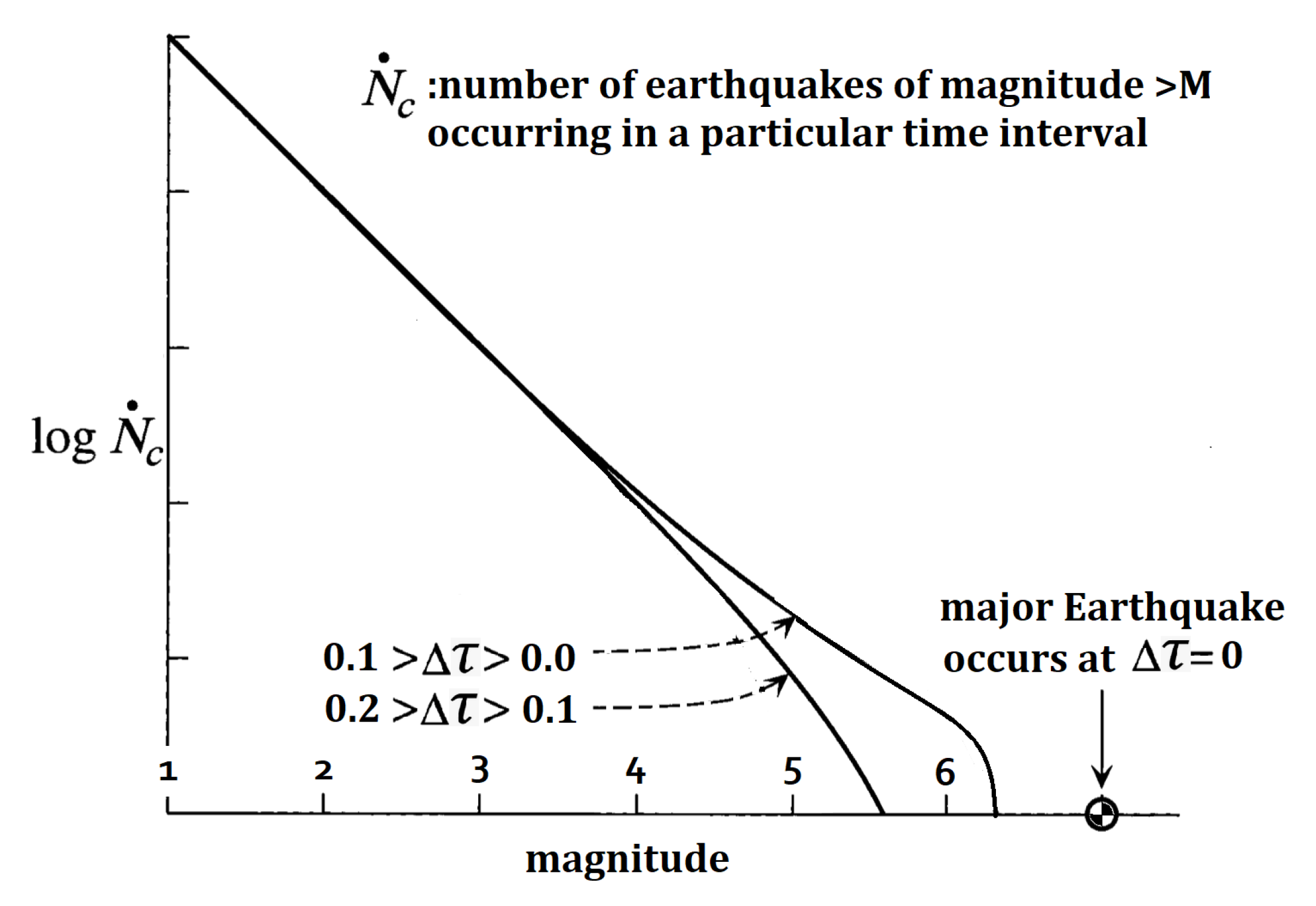
Figure 2.
Cracks of length R separated by uncracked material of diameter D [22].
Figure 2.
Cracks of length R separated by uncracked material of diameter D [22].
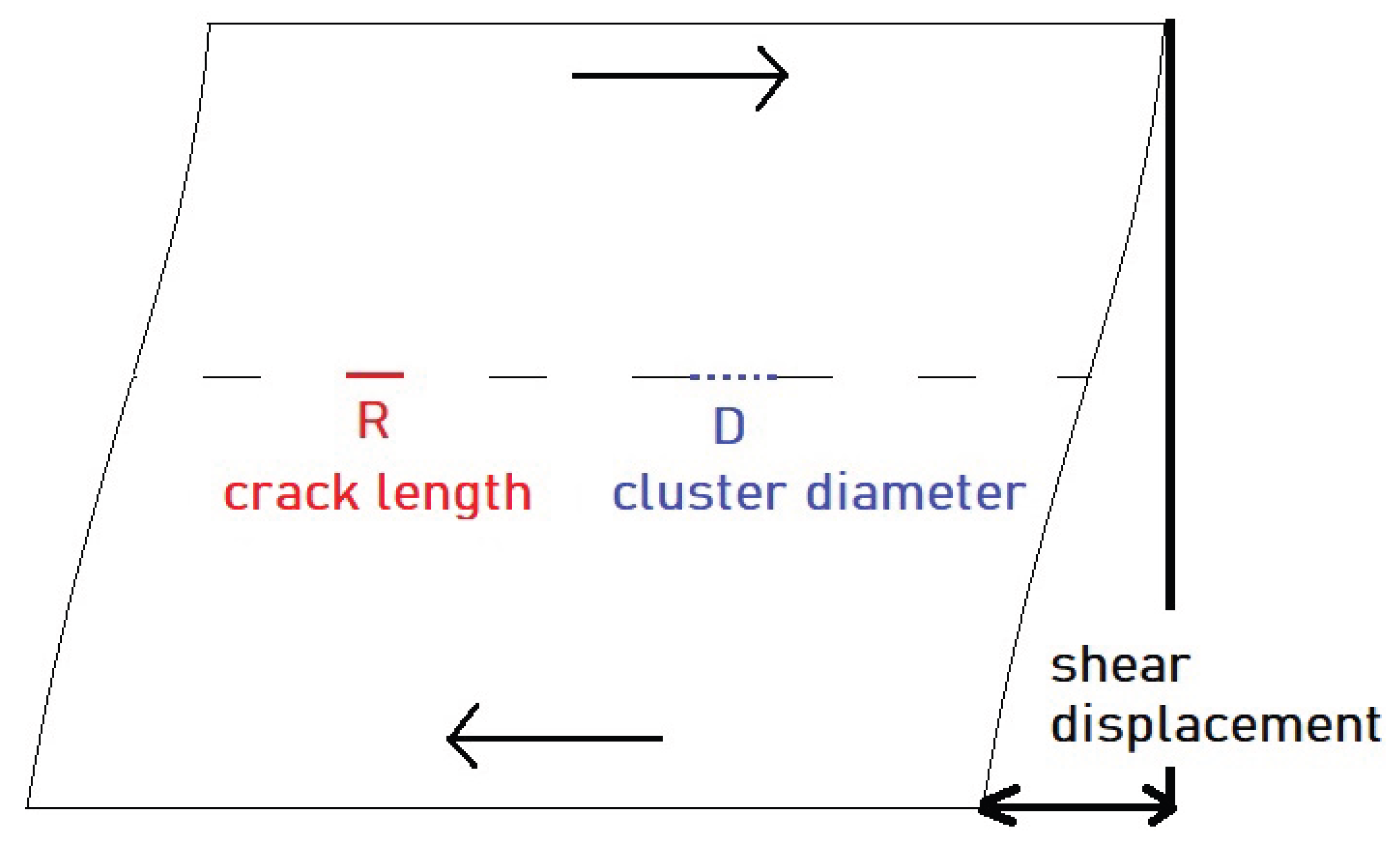

Table 1.
Approximate relation between earthquake magnitude, fault material displacement, and fault rupture length.
Table 1.
Approximate relation between earthquake magnitude, fault material displacement, and fault rupture length.
| Moment Magnitude | Average Fault Material Displacement (m) | Fault Rupture Length (km) |
|---|---|---|
| 4 | 0.05 | 1 |
| 5 | 0.15 | 3 |
| 6 | 0.5 | 10 |
| 7 | 1.5 | 30 |
| 8 | 5 | 100 |
Disclaimer/Publisher’s Note: The statements, opinions and data contained in all publications are solely those of the individual author(s) and contributor(s) and not of MDPI and/or the editor(s). MDPI and/or the editor(s) disclaim responsibility for any injury to people or property resulting from any ideas, methods, instructions or products referred to in the content. |
© 2025 by the authors. Licensee MDPI, Basel, Switzerland. This article is an open access article distributed under the terms and conditions of the Creative Commons Attribution (CC BY) license (http://creativecommons.org/licenses/by/4.0/).
Copyright: This open access article is published under a Creative Commons CC BY 4.0 license, which permit the free download, distribution, and reuse, provided that the author and preprint are cited in any reuse.


