Submitted:
22 January 2026
Posted:
22 January 2026
You are already at the latest version
Abstract
2D elastostatic displacement solutions for the Yoffe Mode I and Rice Mode II crack models are reviewed. These solutions are used to introduce the elastostatic displacement solution for a 2D Mode I/II multi-crack configuration in terms of meromorphic differential forms on a hyperelliptic curve. The complex dimension of the vector space of mermorphic forms is demonstrated to be g+1, where g is the genus of the hyperelliptic curve, using the Riemann-Roch theorem. Limitations of the 2D multi-crack model to modeling 3D fracture networks are identified, and a mathematical description of 3D fracture network dynamics preceding an earthquake based on singular spectrum analysis of crack phase fields is conjectured.
Keywords:
mode I
; mode II
; multi-crack
; statistics
; singular spectrum analysis
1. Introduction
Analytic solutions for elastostatic displacement due to vertical/shear traction applied to the faces of a single crack in a 2D plane are reviewed in Section 2. The purpose of this review is to introduce mathematics relevant to specifying multi-crack elastostatic displacements. In Section 3, the relation between multi-crack elastostatic displacement fields and Riemann surface geometry is discussed. Section 4 explains why 2D multi-crack solutions appear limited to describe idealized cracks in 2 spatial dimensions, and conjectures how 3D fracture networks in the lithosphere can be described in terms of singular spectrum analysis of crack phase fields.
2. Single Crack 2D Elastostatic Displacement
2.1. Yoffe Mode I Crack
Consider a sharp crack of length R propagating with constant velocity v in a uniform elastic material in 2D plane strain conditions, whereby the crack tips are located at and . In terms of coordinates in which the crack tips are fixed at and , the elastic displacement can be expressed in terms of scalar and vector potentials and as:
where:
for constants and specified by v and the P and SV wave velocities and [7]. In turn, the potentials and can be expressed in terms of analytic functions and as:
for and , whereby elastic displacement field and stress field components are given by the equations:
for Lame parameters and .
Now assume the crack is Mode I, in that a uniform vertical traction acts on the crack faces while the shear traction applied to the crack faces is 0, as illustrated in Figure 1-left. In this case the crack face boundary conditions are:
and the potentials and have the symmetries and imply and , in keeping with x-axis reflection symmetry of a Mode I crack displacement solution. Furthermore, the Cauchy-Riemann equations imply and .
The symmetries of F and G, together with equations (10) and (12), imply the function:
is continuous across the crack line between and , and is therefore entire. Given that the elastic velocity and stress fields are zero at points remote from the crack, Lioiuville’s theorem on bounded entire functions implies:
Equations (9) and (14) together with condition (11) imply:
where , and discontinuity of across the crack line occurs as necessary to account for discontinuity in elastic displacement. Assuming is defined as a single valued function on the complex plane with a branch cut between and along , the function:
is continuous across the crack line, and is therefore an entire function that approaches 0 as , implying:
and:
Equations (17) and (18) imply the normal stress distribution on the crack line ahead of the advancing crack tip is:
Integration of equations (17) and (18) gives equations:
and:
in which constants of integration have been selected so elastic displacements are 0 at remote points. Assuming is defined as a single valued function on the complex plane with a branch cut between and along , equations (20) and (21) together with equation (7) imply the crack opening displacement is:
2.2. Rice Mode II Crack
Now assume the crack is Mode II, in that a uniform shear traction is applied to the crack faces while the vertical traction applied to the crack faces is 0, as illustrated in Figure 1-right[12]. In this case the crack face boundary conditions are:
and the potentials and have the symmetries and so that:
and:
as necessary to satisfy the Cauchy-Riemann equations for analytic functions and .
Equations (27) and (28) imply the function:
is continuous across the crack line, and therefore entire. Furthermore, vanishing of stress and velocity field displacements as imply is bounded at infinity, and thus identically 0 by Liouville’s theorem. Consequently:
which together with boundary condition (23) implies that along the crack line:
where , and discontinuity of across the crack line occurs as necessary to account for discontinuity in elastic displacement. Assuming is defined as a single valued function on the complex plane with a branch cut between and along , the function:
is continuous across the crack line, and is therefore an entire function that approaches 0 as , implying:
and:
Integration of equations (33) and (34) gives equations:
and:
in which constants of integration have been selected so elastic displacements are 0 at remote points. Assuming is defined as a single valued function on the complex plane with a branch cut between and along , equations (35) and (36) together with equation (6) imply the crack opening displacement is:
3. Multi-Crack 2D Elastostatic Displacement
3.1. Crack Geometry: Hyperelliptic Curves
For the purpose of calculating multi-crack 2D elastostatic displacements, cracks will be identified with branch cuts of the complex plane specifying sheets of Riemann surfaces. To explain this statement in detail, consider the equation:
relating complex variables Y and with different complex values . For each pair of values the expression:
can be a singled valued analytic function on the complex X-plane with a branch cut joining the points and , and this function is unique up to choice of sign. Iterating selection of a branch for square root for , it the product:
can be defined as a single valued analytic function on the complex X-plane, up to choice of sign, away from a finite set of branch cuts joining branch points and in pairs. For this reason, the projection:
from points satisfying equation (38) to the complex X-plane is a double cover of the complex plane away from the branch cuts.
The projective completion of non-compact hyperelliptic curve (38) is the compact hyperelliptic curve:
in . From this point of view, the projection:
from points on curve (42) to the Riemann sphere is a double cover with branch points at . When , equation (42) implies:
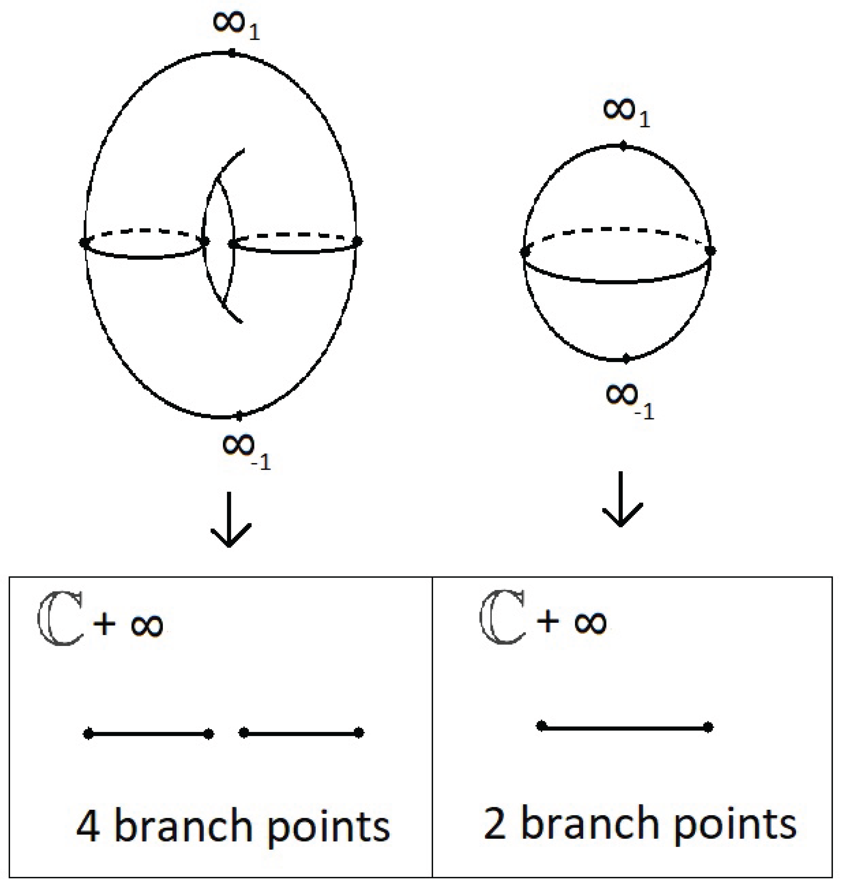
so the point with is covered by the two points . Therefore, for the point at infinity is double covered by and while for the point at infinity is double covered by . With resolution of the singularity at , projection (43) can be drawn as a projection from a non-singular genus g Rieman surface to the Riemann sphere as shown in Figure 2. In this image, the inverse image of each branch cut is shown as a closed loop on the surface.
3.2. Elastostatic Displacement: Differential Forms
For a superposition of vertical/shear traction acting on the crack faces, the Mode I and Mode II single crack elastostatic displacement potentials and independently solve the 2D Laplace equation:
away from the crack lines in the and planes. By Gauss’ and Stokes’ theorems, the line integrals:
and:
each obtain a constant value for any closed contours and encircling the crack once counterclockwise in the and planes. Moreover, these constant values can be non-zero because the analytic functions and are multi-valued, as may be anticipated based on dependence of elastostatic displacement at points remote from the cracks. This dependence can be extracted from singular behavior of differential forms and at infinity evaluated using the substitution . Noting that:
for , and , it is evident that both and have a simple pole at infinity. For this reason, the integral of the pullback of either form to a Riemann sphere around the closed contour shown in Figure 2 is non-zero, because the form has a simple pole on both the inside and outside of the contour.
For , cracks in the or plane can be viewed as branch cuts for a double cover of the plane by a hyperelliptic curve of genus g, and multi-crack elastostatic displacement solutions for constant vertical or shear surface tractions are associated with meromorphic 1-forms on the curve. The Riemann-Roch theorem applies to calculate the dimension of the complex vector space of meromorphic 1-forms on a non-singular Riemann surface of genus g with simple poles at 2 prescribed points as being . More specifically, the theorem for curves states that if is a canonical divisor on a non-singular Riemann surface of genus g, then:
where is the complex dimension of the vector space of meromorphic functions on the Riemann surface bounded by divisor D[8]. Consequently, if an elastostatic displacement vector field in the multi-cracked plane is associated with meromorphic 1-forms and in the and planes via Helmholtz decomposition (1) and equations (4) and (5), the pullback of either 1-form to a non-singular genus g Riemann surface can each be expressed as a linear combination of a basis , , ..., , for a vector space of mermomorphic 1-forms on the respective curve, where each is holomorphic and has simple poles at the points . When , the and planes coincide and both meromorphic 1-forms and pullback to 1-forms on the same Rieman surface. In this case, the complex dimension is in agreement with the fact there are real parameters and available to specify constant vertical and shear surface tractions on crack faces of the multi-crack system, since the elastostatic displacement fields associated with sets of constant surface tractions form a real vector space.
4. 3D Fracture Networks
Correspondence between 2D multi-crack configurations with hyperelliptic curves suggests a change in 2D crack configuration (e.g. crack growth) may be modeled as a change in the shape of a Riemann surface. This fact is of scientific interest because current methods of modeling and simulating crack growth invoke empirical time evolution equations for crack phase fields (i.e. damage fields), and these methods may be advanced by more systematic time evolution modeling [9]. However, practical application of the multi-crack Riemann surface model to modeling crack growth in laboratory rock samples and the lithosphere appears lacking for at least two reasons:
- It is not clear how the 2D Riemann surface model can be generalized to describe cracks of arbitrary orientation and finite width in 3 spatial dimensions.
- It is not clear how the 2D Riemann surface model can be generalized to describe elastostatic displacement of a material whose elastic parameters vary in space and time.
To address these problems, an introductory discussion of 3D fracture in laboratory rock samples and the lithosphere is presented, and 3D fracture network dynamics preceding an earthquake are characterized in terms of singular spectrum analysis of a crack phase field. Physically, specification of a crack phase field in a laboratory rock sample or region of the lithosphere adjusts material elastic parameters based on crack damage, with an increase in the crack phase field at a particular spatial location corresponding to a reduction in elastic shear modulus of material. Within the lithosphere, changes in material shear modulus can be detected as changes in local earthquake coda wave signals on seismograms, allowing for detection of a fault damage zone formed before earthquake fault rupture. Conjecturally, time evolution of the crack phase field preceding an earthquake is governed by a finite dimensional nonlinear dynamical system with phase space dimension equal to a number of dynamic modes of fault damage. From this point of view, it remains possible that the underlying nonlinear dynamical system phase space of a 3D crack phase field is related to the geometry of Riemann surfaces, although more detailed investigation is required to determine whether or not this is the case.
4.1. Laboratory Rock Fracture
Consider a triaxial compression test on a rock sample for which axial compressive strain is applied along principal axis 1 while compressive stresses in the direction of principal axes 2 and 3 are held constant. Assume the initial compressive stresses satisfy , and as is increased towards a maximum value , plastic strain hardening of the rock sample occurs. Also assume that when is increased beyond the strain at which , strain softening of the rock occurs with formation of a shear band along a plane where the rock ultimately undergoes shear failure. Technically, the constitutive model of the rock may be defined using a Mohr-Coulomb yield criterion with mobilized friction angle/cohesion and a non-associated plastic flow rule [15].
Physically accurate and well defined mathematical description of the rock strain softening regime requires addition of at least two features to the strain hardening non-associated plasticity model:
If it is assumed that with consideration of these technical details, and definition of a finite element mesh, a global elasto-plastic tangent stiffness operator can be defined for the rock sample throughout triaxial compression at a constant strain rate at each time , Newton’s equation of motion dictates that the equation:
describes time evolution of a vector perturbation to the finite element nodal elasto-plastic displacements at time , where M is a lumped mass matrix, is a damping matrix at time , and is a perturbation of the externally applied nodal force vector [4].
4.2. Lithospheric Fracture Networks
Typically, plastic deformation of rock material occurs with cracking (i.e. damage). In seismology, earthquake faults are observed to be surrounded by damage zones, and detecting fault damage zone formation by monitoring real time variation of local earthquake coda wave signals on seismograms has been identified as a possible method of predicting earthquakes [1]. According to this method, in a frequency band centered at angular frequency , time variation of the local earthquake coda value at a particular seismic station can be attributed to time variation of the anelastic and/or scattering Q values and according to the equation:
and decrease of in time may reflect earthquake precursor dynamics in the lithosphere. More specifically, based on a single backscattering model of coda wave signals, scales with signal frequency according to the power law:
and may therefore contribute to real time variation of if the Hurst exponent H changes in time [16]. Fundamentally, the Hurst exponent H is related to the power spectrum of random S-wave velocity model inhomogeneities in the lithosphere , where k is wave number, via the relation [14]:
These random inhomogeneities can be attributed to a fracture network superimposed on a fixed seismic velocity model background, such as a 1D layered velocity model, with fracture size statistics characterized by equation (57).
4.3. Crack Phase Field Singular Spectrum Analysis
Suppose a scalar crack phase field influences Lame elastic parameters and of a 3D laboratory rock sample or lithospheric region via the equations:
where and are the Lame parameters of uncracked rock at location , is the crack phase field with value 0 for uncracked material and 1 for maximally damaged material, and and are constants [10]. If the crack phase field can be directly measured at a particular 3D location P at regular time intervals, the sequence of phase field values can be used to write a trajectory matrix :
whose singular value decomposition can be used to identify dominant signal components in the discrete time series [5]. More generally, the scalar time series can be replaced with a vector time series of phase field values at different 3D locations, and multichannel singular spectrum analysis can be applied to identify dominant vector signal components in the time series.
Realistically, crack phase field values are not measured at individual points in a laboratory sample or the lithosphere, but may be inferred from changes in local earthquake coda wave signals. Therefore, it is noted that single/multi-channel singular spectrum analysis allows for replacement of the scalar/vector time series of crack phase field measurements with a scalar/vector time series of experimentally observed data, such as relative changes in average S-wave velocity between seismic station pairs measured by monitoring coda wave signals [11]. It is conjectured that each is the measurement of an observable on a nonlinear dynamical system with a finite dimensional phase space , whereby the rows of the trajectory matrix provide an embedding of the phase space trajectory in into . Based on this conjecture, an estimate of the dimension of the phase space trajectory in is provided by computing the correlation dimension of the phase space trajectory embedded in .
The conjectured existence of a finite dimensional nonlinear dynamical system describing time evolution of the fault damage zone is a generalization of a previous claim by seismologists that the average damage along an earthquake fault preceding its rupture evolves according to a 1 dimensional nonlinear dynamical system [3]. From this point of view, if the damage field can be decomposed into a linear superposition of finitely many time independent damage modes with time dependent coefficients :
a nonlinear dynamical system:
specifies time evolution of the phase field and is contained in . So that each damage mode is associated with localization of strain in the lithosphere, it is further conjectured that each damage modes corresponds to a nodal displacement eigenvector of an elasto-plastic stiffness matrix with complex eigenvalue satisfying . Whether or not there is good reason to identify the eigenvalues as branch points of a cover of the complex plane by a -dependent Riemannn surface remains unclear.
5. Conclusions
Further computational and experimental effort is required to distinguish fundamental models of crack growth models based on applied mathematics from those based on mathematical concoction. In particular, an example of simulating crack phase field time evolution in a laboratory rock sample and using singular spectrum analysis to characterize this time evolution should be provided to clarify what dynamical system governs damage time evolution. If the results of an initial computational investigation are promising, an example of using singular spectrum analysis of coda wave data to specify a finite dimensional nonlinear dynamical system should be provided as evidence for real world applicability of the signal processing method. Theoretically, to the point of providing deterministic or probabilistic analytic models of phase field time evolution, it may be useful to investigate if time evolution of an elasto-plastic tangent stiffness matrix eigenvalue distribution can be cast in terms of statistical mechanics of a 2D Coulomb gas [13].
Acknowledgments
Thanks to my family for their support during completion of this research.
References
- Aki K Theory of earthquake prediction with special reference to monitoring of the quality factor of lithosphere by the coda method. In Practical Approaches to Earthquake Prediction and Warning; Springer Netherlands: Dordrecht, 1 Jan 1985; pp. 219–230.
- Behn, MD; Lin, J; Zuber, MT. A continuum mechanics model for normal faulting using a strain-rate softening rheology: Implications for thermal and rheological controls on continental and oceanic rifting. Earth and Planetary Science Letters 2002, 202(3-4), 725–40. [Google Scholar] [CrossRef]
- Ben-Zion Y, Lyakhovsky V Accelerated seismic release and related aspects of seismicity patterns on earthquake faults. Pure and Applied Geophysics 2002, 159(10), 2385–412. [CrossRef]
- Bindel DS Structured and parameter-dependent eigensolvers for simulation-based design of resonant MEMS. Doctoral dissertation, University of California, Berkeley, 2006.
- Broomhead DS, King GP Extracting qualitative dynamics from experimental data. Physica D: Nonlinear Phenomena 1986, 20(2-3), 217–36. [CrossRef]
- Carlson, JM; Langer, JS; Shaw, *!!! REPLACE !!!*. Dynamics of earthquake faults. Reviews of Modern Physics 1994, 66(2), 657. [Google Scholar] [CrossRef]
- Freund LB Dynamic fracture mechanics; Cambridge university press, 1998.
- Griffiths P,Harris J Principles of algebraic geometry, Pure and Applied Mathematics; John Wilney and Sons: New York, 1978.
- Kuhn C, Müller R A phase field model for fracture. In InPAMM: proceedings in applied mathematics and mechanics; WILEY-VCH Verlag: Berlin, Dec 2008; Vol. 8, No. 1, pp. 10223–10224.
- Lyakhovsky V, Ben-Zion Y, Agnon A Distributed damage, faulting, and friction. Journal of Geophysical Research: Solid Earth 1997, 102(B12), 27635–49. [CrossRef]
- Merrill, RJ; Bostock, MG; Peacock, SM; Chapman, DS. Optimal Multichannel Stretch Factors for Estimating Changes in Seismic Velocity: Application to the 2012 M w 7.8 Haida Gwaii Earthquake. Bulletin of the Seismological Society of America 2023, 113(3), 1077–90. [Google Scholar] [CrossRef]
- Rice, JR; Simons, DA. The stabilization of spreading shear faults by coupled deformation-diffusion effects in fluid-infiltrated porous materials. Journal of Geophysical Research 1976, 81(29), 5322–34. [Google Scholar] [CrossRef]
- Saleur H, Sammis CG, Sornette D Renormalization group theory of earthquakes. Nonlinear Processes in Geophysics 1996, 3(2), 102–9. [CrossRef]
- Sato H Power spectra of random heterogeneities in the solid earth. Solid Earth 2019, 10(1), 275–92. [CrossRef]
- Vermeer PA Non-associated plasticity for soils, concrete and rock. In Physics of dry granular media; Springer Netherlands: Dordrecht, 30 Jun 1998; pp. 163–196.
- Wu RS, Aki K The fractal nature of the inhomogeneities in the lithosphere evidenced from seismic wave scattering. Pure and applied geophysics 1985, 123(6), 805–18. [CrossRef]
Figure 1.
Stationary Yoffe Mode 1 crack (left) and Rice Mode II crack (right).
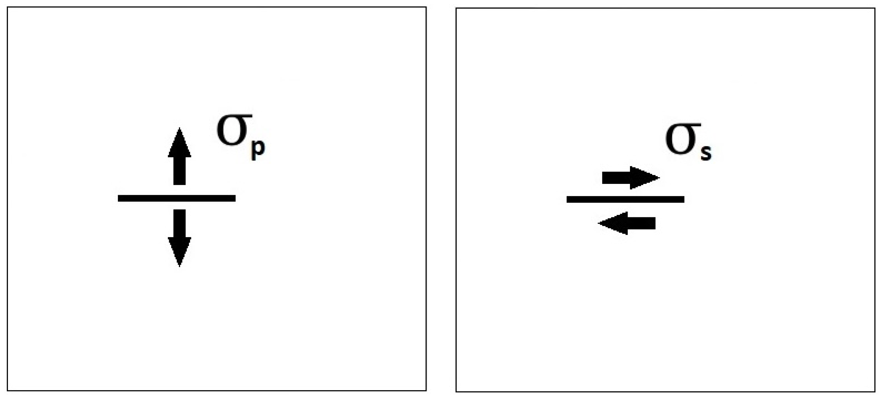
Figure 2.
Double cover of Riemann sphere () by genus 1 and genus 0 hyperelliptic curves with 4 and 2 branch points.
Figure 2.
Double cover of Riemann sphere () by genus 1 and genus 0 hyperelliptic curves with 4 and 2 branch points.
Disclaimer/Publisher’s Note: The statements, opinions and data contained in all publications are solely those of the individual author(s) and contributor(s) and not of MDPI and/or the editor(s). MDPI and/or the editor(s) disclaim responsibility for any injury to people or property resulting from any ideas, methods, instructions or products referred to in the content. |
© 2026 by the authors. Licensee MDPI, Basel, Switzerland. This article is an open access article distributed under the terms and conditions of the Creative Commons Attribution (CC BY) license (http://creativecommons.org/licenses/by/4.0/).
Copyright: This open access article is published under a Creative Commons CC BY 4.0 license, which permit the free download, distribution, and reuse, provided that the author and preprint are cited in any reuse.


