Submitted:
07 February 2025
Posted:
07 February 2025
You are already at the latest version
Abstract
With the increase in population in certain urban areas, resulting in the sometimes uncontrolled expansion of cities, the increase in water requirements and the multiplication of sources of groundwater pollution, it is very important to know the boundaries of even the most complex aquifers in the world in order not only to guarantee their sustainable use, but also to keep them at a safe distance from sources of pollution, especially anthropogenic. Many of the world's cities draw their water from great distances because the aquifers they contain were not identified and preserved at the time they were built and developed. Just as it can be difficult to know the geometry of pollution sources, it is equally complex to know the geometry of aquifers, especially in granitic or gneissic bedrock. This paper examines the impact of uncontrolled urbanisation on potential aquifers. To do this, it uses an approach that integrates field and remote sensing data in the Analytic Hierarchy Process (AHP) through Geographic Information Systems (GIS), combined with piezometry data used in a clusterisassion to delimit potentially aquiferous zones in an environment characterised by poorly controlled urban growth. This approach uses spatial representation to delimit potentially aquiferous zones in urban and peri-urban environments. Given the anarchic nature of certain urban developments, this work shows that several aquifers in many urban areas may still be threatened by anthropogenic pollution and deserve to be preserved. Furthermore, the preservation of these aquifers in urban and peri-urban areas seems to require more urgent and robust policies from both governments and development partners if they are to be preserved and used sustainably.
Keywords:
Remote sensing and GIS
; AHP
; Groundwater forecast maps
; cluster
; urbanisation
; pollution
1. Introduction
Groundwater is very important for towns and suburbs [1,2,3,4,5,6,7,8,9,10]. In a number of countries around the world, many NGOs and donors are spending a lot of money to help people build wells and boreholes to supply themselves with water [3]. If the reservoirs that supply these cities are not preserved, all this investment and aid will have no effect. What's more, some cities, such as New York, Shanghai, Tokyo, Paris, Lisbon, London and Berlin, are spending colossal sums to draw their water supplies from several kilometres away [11,12]. Studies [8,11,12,13,14,15,16,17,18,19,20,21,22,23] show that the preservation of aquifers in the face of urban and demographic growth worldwide remains a major concern. To achieve the targets set out in the 2030 WHO roadmap [22], it is very important to know the boundary between latrine pits and aquifers. While it is easy to know the geometry of latrine pits, it is complex to know the geometry of aquifers, especially in gneissic and alteritic basement environments. This paper examines the impact of uncontrolled urbanisation on potential aquifer areas. To do this, it uses and tests an approach that integrates field and remote sensing data in the AHP through GIS, combined with piezometry data used in a clusterisation to delimit potential aquifer zones in the face of uncontrolled urban thrust. This approach uses spatial representation to juxtapose the potential aquifer zones identified in relation to urban and peri-urban areas.
2. Material and Method
2.1. Materials
2.1.1. Study Area
The study area is located between latitudes 3°42’ and 3°57’ North, and longitudes 11°24’ and 11°34’ East with an estimated population of 4,509,287 in 2023 according to World Population Review, spread over an area of 289 km², compared with 3,096,782 in 2015 (Figure 1). It is undergoing rapid and uncontrolled urbanisation where buildings are built on one level, destroying vegetation, wetlands and waterways as in some of the world's cities… The altitude of the study area varies from 630 to 1200 m above mean sea level (masl). Normal annual rainfall varies from 20 to 290 mm, the average minimum temperature is about 18°C and the average maximum temperature is 28°C. There are 4 main seasons including 2 rainy seasons (major and minor) and 2 dry seasons (major and minor).
2.1.2. Thematic Layers
Geological setting
According to [23], the Precambrian basement of southern Cameroon comprises several metamorphic series (Figure 2). The Yaounde series, affected by the Pan-African orogeny (600 and 500 My), is mainly composed of gneisses and garnet migmatites, derived from ancient granitised and metamorphosed sediments [24]. This series consists of two major migmatitic units [24]: a meta-sedimentary unit or paragneiss and a metaplutonic unit or orthogneiss (Figure 2). The paragneisses are mainly composed of garnet and disthene gneisses, garnet and plagioclase gneisses, marbles and scapolitic rocks. The orthogneisses are characterised by intrusive pyriclasites in the metasedimentary unit, garnet pyribolites, pyroxenites and biotite rich rocks.
Geomorphology
Geomorphological units are important aspects of the physical characteristics of the land surface, estimation of topography, hydrogeological investigations and identification of groundwater resources [25]. The South Cameroon plateau is a platform with an average altitude of 700 m (Figure 3) (Table 1). The most remarkable gneissic massifs, which reach an altitude of over 1000 m, are found to the west of the study area. Geomorphological studies, particularly those on orography, show that these massifs are concentric and thus describe a multi-circular structure 19 km in diameter and 418 m deep, located to the south-east of the elliptical depression of the study area. Two rings are highlighted, an outer, almost circular ring of 19 km in diameter and an inner circular ring of 8 km in diameter eccentric to the south. These rings are separated by valleys of descending centripetal elevations illustrating a stepped relief. Hydrographic analysis reveals a general dendritic network, supported by rectangular, collinear and parallel networks. At the level of the circular structure, a particular radial and circular network is established, characteristic of the above-mentioned rings. This evidence of radial and circular hydrography coupled with the massive ring arrangement, confirms the presence of a closed, circular, multi-ringed depression in the western sector of the study area whose ramparts correspond to the highest surface of the southern Cameroonian plateau.
Land Use and Land Cover (LULC)
The LULC map is important for monitoring soil water infiltration rates and surface runoff [26,27]. It is derived from Landsat 8 satellite imagery (OLI), prepared and interpreted using classification in ArcGIS 10.5 and plays an important role in the existence and development of groundwater. In the study area, the classification of the different LULCs was done in five main categories (Figure 4). It was found that wetlands occupy an area of 19.8 km2, built-up areas 28 km2, wastelands 62.70 km2 and agricultural land 201.3 km2 (Table 2), which shows that built-up areas and agricultural land reduce the recharge rate of groundwater and runoff [28].
Density of lineaments
Lineament refers to linear or curvilinear surface features such as crustal fractures, shear zones, faults, rift zones, bedding and major tectonic boundaries [29,30,31]. The density of lineaments in the research area varies from 0.00 to 7.19 km/km2. Five main classifications were made for these lineament densities; 0.00-1.43; 1.43-2.87; 2.87-4.31; 4.31-5.75; 5.75-7.19. The areas with high lineament density show a high potential for groundwater prosperity. In contrast, areas with less lineament density on the map show poor groundwater potential (GWP) [32]. Figure 5 shows the lineament density of the study area and Table 3 shows the different lineament density classes.
Drainage density
On the other hand, a high drainage density will be conducive to high water runoff, and therefore this type of area shows a low water potential. Low drainage density allows less water runoff and shows good GWP [33,34,35]. Drainage density in this study varies from 0.00 to 17.18 km/km2 and is divided into five categories such as 0.00 to 1.54 km/km2; 1.54 to 4.10 km/km2; 4.10 to 6.87 km/km2; 6.87 to 9.97 km/km2 and 9.97 to 17.18 km/km2 (Figure 6). The Table 4 represents the drainage density attributes.
Slopes
Figure 7 shows that the slopes of the region have a direct impact on water infiltration [35,36] and the distribution by area of each slope class is shown in Table 5. They vary from 0.00° to 38.58° and are subdivided into three main classes which are (1) steep slopes (19.36° to 38.58°), which are given the lowest ranking for GWP. The rate of water infiltration in this area becomes much lower and causes high runoff; (2) the medium slopes (3.48° to 19.36°) of medium GWP; (3) the lesser slopes (0.00° to 3.48°) are assigned the highest ranking due to high water infiltration. All these results show that slopes in the study area have a direct impact on water infiltration [33].
2.2. Method
2.2.1. Analytic Hierarchy Process (AHP)
AHP is a widely used and reliable method for assigning weights to several criteria in spatial decision-making [36,37]. It involves a pairwise comparison method in which each criterion is given a score relative to the other criteria, followed by a valid consistency check [37,38].
Influencing factors for GWP zones
This study uses and tests an approach that integrates remote sensing and field data in the AHP through GIS, combined with piezometry data used in a clusterisation to delineate aquifer zones in an alteritic complex. To achieve this, Six influencing parameters such as geology (GE), elevation (EL), slope (SL), LULC, lineament density (LD) and drainage density (DD) were considered. Their thematic maps were analysed according to the Multi-Criteria Decision Making (MCDM) and AHP using standardised weights to evaluate the groundwater exploration areas. A geological map acquired from the Geological and Mining Research Institute of Cameroon (IRGM) was used. The topographic elevation maps, Drainage network, and slope of the study area, drawn by the SRTM DEM model at 30 m spatial resolution. The lineament density map of the study area was generated from Landsat-8 (OLI (January 2020)) satellite imagery assessed by the United States Geological Survey (http://earth explorer.usgs.gov) with a spatial resolution of 30 m. Automatic lineament extraction was performed using the lineament module of the PCI Geomatica software package [41]. In the present study, the LULC map was prepared at 1: 25,000 scale from the Landsat-8 TM image using image interpretation features such as tone, texture, drainage and relief. In the study area, the land use classification and land cover map were supervised by a learning classification method using the maximum likelihood classifier (MLC) in ArcGIS 10.5 (Table 6, Table 7), where each parameter was assigned a specific weight according to its relative importance in determining the presence of groundwater from the AHP (Table 7) [35,36,40,41,42].
The criteria were compared in pairs using the Saaty scale for each level of the hierarchy (Table 6). This scale, ranging from 1 to 9, expresses the intensity of preference of one criterion over another.
Pair-wise comparison matrix
Where bij are 1 for i=j and indicate equal importance between criteria and are greater than 1 for i≠j in case of importance.
Estimation of relative weights
The pairwise comparison matrix (Table 7) is normalised (Table 8) to obtain relative weights. The theme element values were divided by the sum of the values in the corresponding column of the pairwise comparison matrix as in equation (5) [35,36,37,40,41,42].
Where Bij are the elements of the peer comparison matrix, Tij the total of the elements of the corresponding column of said matrix and Dij represents the normalised peer comparison matrix. [35,36,37,40,41,42].
To find an average value for i in equation (6), each normalised pairwise matrix member is divided by n.
Ci represents a certain typical mass. The eigenvectors and eigenvalues are essential for determining constraints and determining the relative importance of the topic layer. To determine the eigenvector, the sums of the columns are divided by the number of items in the columns. The fundamental eigenvector was computed by arithmetically averaging the rows, so revealing the relative importance of each parameter. Using equation (7) to construct a stable vector, the values of a normalised pairwise matrix was multiplied by a pairwise comparison matrix based on selected thematic layers [35,36,37,40,41,42].
Delineation of Groundwater Potential Zone (GWPZ)
GWPZ represent dimensionless areas that predict the potential groundwater zones in a region [43]. The total GWP map was created when the raster calculator tool in the ArcGIS 10.5 environment was used to execute Equation (9). Information from the aforementioned layers was combined in the ArcGIS environment to create the GWPZ map [44].
Where Wi is the normalised weight of the thematic layer j, Xj is the rank value of each class with respect to layer j, m is the total number of thematic layers and n is the total number of classes in a thematic layer. The GWPI for each grid was calculated using equation (2):
Where GEw and GEr are the weight of a feature and the rate of geology, SCW and SCr are the weight of a feature and the rate soil cover , DDw and DDr are the weight of a feature and the rate of drainage , SLw and SLr are the weight of a feature and the rate of slope , LCw and LCr are the weight of a feature and the rate of land cover ,LDw and LDr are the weight of a feature and the rate of lineament density, GMw and GMr are the weight of a feature and the rate of geomorphology individual subclasses of a feature according to their relative importance for groundwater potentiality; LC, land cover; DD, drainage density; SL, slope; SC, soil cover; LU, land use; LD, lineament density; and GM, geomorphology. The indices "w" and "r" representing the rating ranges of 1 to 5 were considered, where the scores of 1, 2, 3, 4 and 5 represent very poor, poor, moderate, good and very good, respectively, in terms of groundwater storage potential [28].
Assignment and normalisation of weights
The assignment of standardised weights using the AHP was developed by [37]. This AHP method is a widely used MCDM procedure for natural resources, land suitability analysis and ecological risk assessment. The GIS-based AHP technique has been developed by the international academic network as a key asset for studying complex spatial choice issues [43]. The comparison scores are on the Saaty scale from 1 to 9 [37]. The highest weights were assigned to the themes of good groundwater potentiality and the lowest weights to poor groundwater potentiality. To determine the weight of each thematic layer, comparison scores on the Saaty scale were prepared and filled in by experts (hydrogeologists, geologists, etc.) from the study area. The final weights of the themes and their characteristics were standardised by adopting the MCDM technique (i.e., the AHP technique proposed by Saaty). The AHP strategy normalises the assigned weights using the eigenvector technique, which reduces the bias/subjectivity involved in the assigned weights. The consistency of the normalised weights was checked by calculating the consistency ratio for different themes and their characteristics [18,37] recommended that the assigned weights should be consistent only when the consistency ratio remains within 10%, otherwise the weights should be reconsidered to remove the irregularity. The calculation of the consistency ratio is done in three steps: (1) the principal eigenvalue (λmax) was calculated by the eigenvector technique, (2) the coherence index (CI) was calculated as follows [37].
Where n is the number of factors
The consistency ratio is obtained by:
RI being the random coherence index for n criteria.
Standard weights for thematic layers
Weights were assigned to the thematic layers as shown in the Table 9, the normalised peer comparison matrix (Table 8) and the different weights were obtained (Table 9) [15]. The assignment of scores to the classes in a thematic layer is related to their relative importance for GWP. Scores from 1 to 5 were selected, where scores 1, 2, 3, 4 and 5 represent very poor, poor, moderate, good and very good groundwater storage potential respectively. As stated in the procedure, the standard weights of the seven themes and their characteristics are obtained using the AHP and Saaty's eigenvector technique (reference). All thematic layers were then analysed against each other in a pairwise comparison matrix and the calculation of standard weights for the different themes using AHP as shown in Figure 8. The thematic layer classes for all parameters and their corresponding evaluations are presented in Table 9. The average value of the coherence vector is 0.025. The value of the coherence index (CI) is 0.031. This shows that there is a significant dimension of coherence in the pairwise comparison, and thus the weights assigned to the different themes are 0.04, 0.07, 0.10, 0.17, 0.24 and 0.37 (i.e., 4%, 7%, 10%, 17%, 24% and 37%) can be assigned to geology, drainage density, slope, LULC, linear density and geomorphology, respectively (Figure 8).
The method of delineating the groundwater exploration areas in the study area, demonstrated using a workflow diagram, is shown in (Figure 8). The groundwater exploration areas were influenced by factors such as geology, geomorphology, land use and cover, slope, lineament density and drainage density [8]. These thematic layers were converted into a raster format and re-ranked according to the assigned weight. Appropriate weights and ranks were assigned to each influence factor and its sub-classes in the thematic layers. These weights were assigned based on their suitability for groundwater storage and flow and the various control factors, and the weights were therefore linked to previous literature reviews and expert opinion. The weights for each thematic layer and its classes, with higher weights or ranks indicating high GWP and lower weights indicating low GWP [28]. The integration of all thematic layers and their weights were calculated by weighted summation and product analysis in the GIS platform [19].
The piezometric map was obtained by ordinary kriging after testing several variogram models by cross-validation using 14 of the 173 points in total. With a standard error of 2.26 m, the spherical variogram was the most appropriate. The cluster logic technique is a procedure that classifies variable objects into groups (clusters) based on similarity or dissimilarity. Cluster analysis involves computational procedures that aim to reduce a data set to several relatively homogeneous groups. The similarity of objects is studied by the degree of similarity (correlation coefficient and/or association coefficient) or by the degree of distance dissimilarity (distance coefficient). Cluster analysis methods are based on clusters classified as hierarchical or non-hierarchical methods. Hierarchical cluster analysis methods consider analysed objects in a hierarchical system of clusters. This system is defined as a system of mutually distinct non-empty subsets of the initial set of objects. The main feature of hierarchical cluster analysis methods creates a decomposition of the initial set of objects, in which each of the partial decomposition clarifies the next or previous decomposition.
2.2.1. Validation of the GWPZ
The aim of the validation is to check whether the GWP model is capable of reproducing variations in piezometry [45].
In other words, we want to see whether the two variables are highly correlated and whether variations in one lead to similar variations in the other.
The data used to assess the relevance of the GWP model are geographical location and piezometry. Principal Component Analysis (PCA) was used to explore the relationships between these four variables. The aim is to reduce the dimensionality of the data and highlight the strongest correlations [45]. All the variables are highly correlated with each other, suggesting that they are linked to the same phenomenon (Table 10). The high correlations between piezometry and GWP (0.9) suggest good agreement between the two variables. This indicates that the potential model is capable of capturing general trends in piezometry. Both variables are strongly correlated with the first factor (geographical factor) (Table 11) suggesting that spatial variations in piezometry are well reproduced by the potential model. The importance of this factor is 78%. The information from this analysis can be seen in Figure 9, which shows the correlations between the variables and the factors (components) in 3D space.
3. Results
3.1. Groundwater Potential Map
The GWPZ Figure 10 were established using equation (2), GIS and AHP techniques. Figure 10 shows the GWPZ grouped into three classes: high potential zones, medium potential zones and low potential zones. Table 12 shows the proportions of each classes. The high potential zones occupy 16.15% of the total area of the study area, the medium potential zones occupy 76.41% and the low potential zones occupy 7.42%. From this distribution, it can be seen that the study area is mainly made up of areas with medium GWP. The high GWPs are mainly located in areas with low slopes, high lineament densities and high drainage densities. Low GWPs are found in areas with steep slopes, low lineament densities and low drainage densities.
Figure 11 shows that 7.42 % of the study area is in poor groundwater distribution, 76.41 % in moderate and 16.15 % in good.
3.2. Result Using Piezometry
3.3. Result Using Cluster
Figure 13 shows the dendrogram which divides the piezometric levels in the area into four classes, each of which illustrates an aquifer. Clusters 2 and 3 are the closest and indicate similar aquifer zones. Clusters 1 and 4 are the furthest away and show two other main aquifer groups.
4. Discussion
The integrated aquifer map presented in Figure 14 shows that there are two aquifers in the north and two aquitards in the south.
This work also shows that the area of maximum drainage correlates with the area of maximum lineament density which coincides with the area of the Mfoundi riverbed, showing that the study area is highly fractured. Figure 15 shows the percentage of water distribution. It can be observed that the study area is characterised by a scarcity of water in aquifers, so it is necessary to preserve the few aquifers that exist, because if the air temperature increases, evapotranspiration will occur and the aquifers will have difficulty being recharged.
It has often been proven that in the basement environments, the areas with a greater density of lineaments when they cross the drainages are areas of water accumulation. Based on this, calculations show that the north and the south of the study area can be favourable to groundwater accumulation. The lineaments play an essential role and north and south of the study area seem to be favourable sectors for groundwater movement due to their high density. The cluster map and the statistical analysis allowed us to find 4 aquifers in the study area.
Combining this map with the map of potential areas, we obtained the integrative aquifer map (Figure 14). This figure shows that the aquifers in the study area are complex. They only share water with the Mfoundi, which is the main collector in the area. This map shows that latrine pits can easily contaminate aquifers. Taking into account the work of [9], we can conclude that there are 4 aquifers in the study area.
Figure 15 and Table 14 show that only 31% of the study area is potentially aquifer-bearing, proving that the aquifers in the area are erratic. Figure 16 shows that urbanisation is becoming increasingly important in areas containing aquifers. Given the anarchic nature of construction, this work shows that these aquifers and many others throughout the world are highly exposed to anthropogenic pollution, requiring more urgent policies from both governments and development partners if they are to be preserved and used sustainably [4,5,7].
5. Conclusion
This paper examines the impact of uncontrolled urbanisation on potential aquifer areas. To do this, it uses and tests an approach that integrates field and remote sensing data in the AHP through GIS, combined with piezometry data used in a clusterisation to delineate potential groundwater zones in the city characterised by uncontrolled urban thrust and rare and erratic aquifers. This approach uses spatial representation to delimit potential aquifer zones in urban and peri-urban environments. Furthermore, the results show that aquifers in cities and peri-urban areas, instead of being protected, are once again under threat from uncontrolled urban growth, raising the question of their sustainable use in particular, and even that of sustainable development in general, if they are to be preserved and used sustainably.
References
- Cairns, J.E.; Hellin, J.; Sonder, K.; Araus, J.L.; Macrobert, J.F.; Thierfelder, C.; Prasanna, B.M. Adapting maize production to climate change in sub-Saharan Africa. Food Secur. 2013, 5, 345–360. [Google Scholar] [CrossRef]
- Kouam, K.G.R.; Djomou, B.S.L.; Rosillon, F. Mutations and the problem of access to drinking water and sanitation in urban area of developing country : the case of the city of Yaounde (centre-Cameroon). Procedings of the 5th international colloquium “water resources and sustainable development” 2013, 764–769.
- https://thedocs.worldbank.org/en/doc/c4d71850a3ffbf182631639b96620723-0330202024/original/La-Note-de-l-Administrateur-no-5-Avril-2024-Eau-ssainissement.pdf.
- WHO (World Health Organization). Report on surveillance of antibiotic consumption: 2016–2018 early implementation 2018.
- UN (United Nations). Sustainable Development Goals Report 2019.
- Dam, Y.; Tiemeni, A.A.; Zing, B.Z.; Nenkam, T.L.L.J.; Aboubakar, A.; Nzeket, A.B.; Mewouo, Y.C.M. Physico-chemical and bacteriological quality of groundwater and health risks in some neighbourhoods of Yaounde VII, Cameroon. IJBCS 2020, 14, 1902–1920. [Google Scholar]
- WHO (World Health Organization). A global overview of national regulations and standards for drinking-water quality. 2nd ed. Geneva: World Health Organization. ISBN 2021, 978-92-4-002364-2.
- Ajay, K.V.; Mondal, N.C.; Ahmed, S. Identification des zones de potentiel des eaux souterraines à l'aide des techniques de RS, SIG et AHP : A Case Study in a Part of Deccan Volcanic Province (DVP), Maharashtra, India. JISRS 2020, 48, 497–511. [Google Scholar]
- Savelli, E.; Mazzoleni, M.; Baldassarre, G. D.; Hannah Cloke, H.; Maria Rusca, M. Urban water crises driven by elites’unsustainable consumption. Nat. Sustain. 2023, 8, 1–12. [Google Scholar]
- Jasechko, S.; Seybold, H.; Perrone, D.; Fan, Y.; Shamsudduh, M.; Taylor, R.G.; Fallatah, O.; Kirchner, J.W. Rapid groundwater decline and some cases of recovery in aquifers globally. Nature 2024, 625–715. [Google Scholar]
- Turner, S.W.D.; Rice, J.S.; Nelson, K.D.; Vernon, C.R.; McManamay, R.; Dickson, K.; Marston, L. Comparison of potential drinking water source contamination across one hundred U.S. cities. Nat. commun. 2021, 12, 7254. [Google Scholar] [CrossRef]
- Hashimoto, R.; Kazama, S.; Hashimoto, T.; Oguma, K.; Takizawa, S. Planning methods for conjunctive use of urban water resources based on quantitative water demand estimation models and groundwater regulation index in Yangon City, Myanmar, J. Clean. Prod. 2022, 367, 0959–6526. [Google Scholar] [CrossRef]
- Teikeu, A.W.; Njandjock N., P.; Tabod, C.T.; Akame, J.M.; Nshagali, B.G. Activité Lineament hydrogeological activity in the Yaounde region of Cameroon using remote sensing and GIS techniques. Egypt. J. Remote Sens. Space Sci. 2016, 19, 49–60. [Google Scholar]
- Prasad, R.K.; Mondal, N.C.; Banerjee, P.; Nandakumar, M.V.; Singh, V.S. Deciphering a potential groundwater zone in hard rock by applying GIS. Environ. geol. 2008, 55, 467–475. [Google Scholar] [CrossRef]
- Meli’i, J.L.; Kouameni, F.V.; Fobissie, L.B.; Teikeu, A.W.; Aretouyap, Z.; Yembe, S.J.; Njandjock, N.P. Hydraulic parameters in the neoproterozoic aquifer of Yaounde, Cameroon. Environ. Earth Sci. 2018, 77. [Google Scholar] [CrossRef]
- Ahmed, R.; Sajjad, H. Analyse des facteurs du potentiel des eaux souterraines et de sa relation avec la population dans le bassin versant du Barpani inférieur, Assam, Inde. Nat. Resour. Res. 2018, 27, 503–515. [Google Scholar] [CrossRef]
- Jha, M.K.; Chowdhury, A.; Chowdary, V.M.; Peiffer, S. Groundwater management and development using integrated remote sensing and geographic information systems: prospects and constraints. Water Resour. Manag. 2007, 21, 427–467. [Google Scholar] [CrossRef]
- Dimitriou, E.; Zacharias, I. Groundwater vulnerability and risk mapping in a geologically complex area using stable isotopes, remote sensing and GIS techniques. Environ. Geol. 2006, 51, 309–323. [Google Scholar] [CrossRef]
- Nobre, R.C.M.; Rotunno, F.O.; Mansur, W.J.; Nobre, M.; Cosenza, C.A. Groundwater vulnerability and risk mapping using GIS, modelling and a fuzzy logic tool. J. contam. Hydrol. 2008, 94, 277–92. [Google Scholar] [CrossRef]
- Machiwal, D.; Rangi, N.; Sharma, A. Integrated knowledge and data driven approaches for groundwater potential zoning using GIS and multi-criteria decision making techniques in the hard rock terrain of Ahar watershed, Rajasthan, India. Environ. Earth Sci. 2015, 73, 1871–1892. [Google Scholar] [CrossRef]
- Swetha, T.V.; Gopinath, G.; Thrivikramji, K.P.; Jesiya, N.P. Combination of geospatial and MCDM tools for identification of potential groundwater prospects in a tropical river basin, Kerala. Environ. Earth Sci. 2017, 76, 428. [Google Scholar] [CrossRef]
- Singh, L.K.; Jha, M.K.; Chowdary, V.M. Accuracy assessment of GIS-based multi-criteria decision analysis approaches for groundwater potential mapping. Ecol. Indic. 2018, 91, 24–37. [Google Scholar] [CrossRef]
- Le Brocque, A.F.; Kath, J.; Reardon, S.K. Chronic groundwater decline a multidecadal analysis of groundwater trends under extreme climate cycles, J. Hydrol. 2018, 4, 59. [Google Scholar]
- Reitzug, F.; Kabatereine, N.B.; Byaruhanga, A.M.; Besigye, F.; Nabatte, B.; Chami, G.F. Current water contact and Schistosoma mansoni infection have distinct determinants: a data-driven populationbased study in rural Uganda. Nat. commun. 2024, 15, 9530. [Google Scholar] [CrossRef]
- Maurizot, P.; Abessolo, A.; Feybesse, J.L.; Lecomte, P.J. Mining prospecting study in Soith-West Cameroon: Summary of work from 1978 to 1985. BRGM report. 1986, 85, CMR–066. [Google Scholar]
- Nzenti, J.P.; Njanko, T.; Njiosseu, E.L.T.; Tchoua, F.M. Granulitic domains of the North Equatorial pan-African chain in Cameroon, J.P. Vicat and P. Bilong (Editors), GEOCAM 1 collection, Yaounde university press, Cameroon 1998, 225-264.
- Krishnamurthy, J.; Srinivas, G. Role of geological and geomorphological factors in ground water exploration: a study using IRS LISS data. Int. J. Remote Sens. 1995, 16, 2595–2618. [Google Scholar] [CrossRef]
- Yimer, F.; Messing, I.; Ledin, S.; Abdelkadir, A. Effects of differents land use types on infiltration capacity in a catchment in the highlands of Ethiopia. Soil Use Manag. 2008, 24, 344–349. [Google Scholar] [CrossRef]
- Gessesse, B.; Bewket, W.; Bräuning, A. Model-Based Characterization and Monitoring of Runoff and Soil Erosion in Response to Land Use/land Cover Changes in the Modjo Watershed, Ethiopia. Land Degrad. Dev. 2015, 26, 711–724. [Google Scholar] [CrossRef]
- Kumar, T.; Tinu, G.A.K. appraising the accuracy of GIS-based multi-criteria decision making technique delineation of groundwater potential zones. Water Resour. Manag. 2014, 28, 13–4449. [Google Scholar] [CrossRef]
- Gweth M.M., A.; Ekoro, N.; Meli’i, J.L.; Gouet, D.H.; Njandjock, N.P. Fractures models comparaison using GIS data around crater lakes in Cameroon volcanic line environment. Egypt. J. Remote Sens. Space Sci. 2017, 419–429.
- Gweth, M.M.A.; Meli’i, J.L.; Oyoa, V.; Ahmad, D.D; Gouet, D.H.; Marcel, J.; Njandjock, N.P. Fracture network mapping using remote sensing in three crater lakes environments of the cameroon volcanic line (Central Africa). Arab. J. Geosci. 14, 422. [CrossRef]
- Poufone, K. Y.; Meli’i, J.L.; Aretouyap, Z.; Gweth, M.M.A.; Nguemhe, F.S.C.; Nshagali, B.G.; Oyoa, V.; Perilli, N.; Njandjock, N.P. Possible pathways of seawater intrusion along the Mount Cameroon Coastal area using remote sensing and GIS techniques. ASR. 2021, 69, 2. [Google Scholar] [CrossRef]
- Horton, R.E. Drainage-basin characteristics. Trans. Am. Geophys. Union. 1932, 13, 350–361. [Google Scholar]
- Das, B.; Pal, S.C.; Malik, S.; Chakrabortty, R. Modelling potential groundwater zones of Puruliya district West Bengal, India using remote sensing and GIS technique. Geol. Ecol. Landsc. 2019, 3, 223–237. [Google Scholar]
- Singh, P.; Hasnat, M.; Rao, M.N. Fuzzy analytical hierarchy processbased GIS modeling for groundwater prospective zones in Prayagraj, India. Groundw. Sustain. Dev. 2021, 12, 100530. [Google Scholar] [CrossRef]
- Pouth, N.A.M; Meli’I, J.L; Gweth, M.M.; Gounou, P.B.P.; Njock, M.C; Teikeu, A.W.; Mbouombouo, N.I.; Poufone, Y.K.; Wouako, W.R.K.; Njandjock, N.P. An approach to assess hazards in the vicinity of mountain and volcanic areas. Landslides 2024. [Google Scholar]
- Vellaikannu, A.; Palaniraj, U.; Karthikeyan, S.; Senapathi, V.; Viswanathan, P. M.; Sekar, S. Identification of groundwater potential zones using geospatial approach in Sivagangai district, South India. Arab. J. Geosci. 2021, 14, 1–8. [Google Scholar] [CrossRef]
- Shebl, A.; Abdelaziz, M.I.; Ghazala, H.; Awad, S.S.A.; Abdellatif, M.; Csámer, A. Multi-criteria ground water potentiality mapping utilizing remote sensing and geophysical data: A case study within Sinai Peninsula. Egypt. J. Remote Sens. Space Sci. 2022, 25, 3–765. [Google Scholar] [CrossRef]
- Saaty, T.L. How to make a decision: The analytic hierarchy process. Eur. J. Op. Res. 1980, 48, 9–26. [Google Scholar] [CrossRef]
- Qari, M.H.T. Linéament extraction from multi- rtésolution satellite imagery: a pilot study on Wadi Bani Malik, Jeddah, Kingdom of Saudi Arabia. Arab. J. geosci. 2011, 4, 1363–1371. [Google Scholar] [CrossRef]
- El Mekki, A.O.; Laftouhi, N.E. Combination of a geographical information system and remote sensing data to map groundwater recharge potential in arid to semi-arid areas: the Haouz Plain, Morocco. Earth Sci. Inform. 2016, 9, 4–465. [Google Scholar] [CrossRef]
- Das, N.; Sutapa, M. Application of multi-criteria making technique for the assessment of groundwater potential zones: a study on Birbhum district, West Bengal, India. Environ. Dev. Sustain. 2018, 22, 2–931. [Google Scholar] [CrossRef]
- Minuyelet, Z.M; Kasie, L.A; Bogale, S. Groundwater potential zones delineation using GIS and AHP techniques in upper parts of Chemoga watershed, Ethiopia. Appl. Water Sci. 2024, 14, 85. [Google Scholar]
- Rahmati, O.; Nazari, S.; Mahdavi, A.; Pourghasemi, M.; Zeinivand, H. Groundwater potential mapping atKurdistan region of Iran using analytic hierarchy process and GIS. Arab. J. Geosc. 2015, 8, 7059–7071. [Google Scholar] [CrossRef]
- Malczewski, J. GIS and multicriteria decision analysis. New York; J. Wiley & Sons., 1999. [Google Scholar]
- Giancarlo, D.; Chiara, T. Cross-validation methods in principal component analysis: a comparison. Statistical methods and applications, J. Italian Stat. Soc. 2002, 11, 1–71. [Google Scholar]
Figure 1.
Map of the study area.
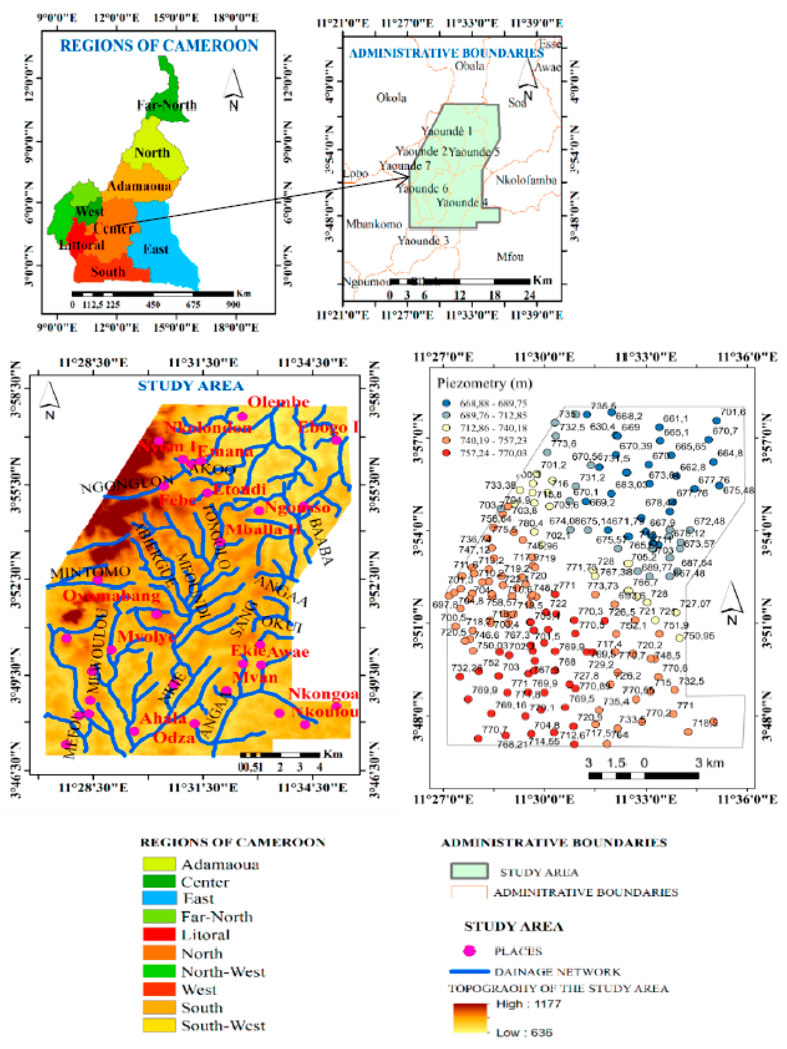
Figure 2.
Geological map.
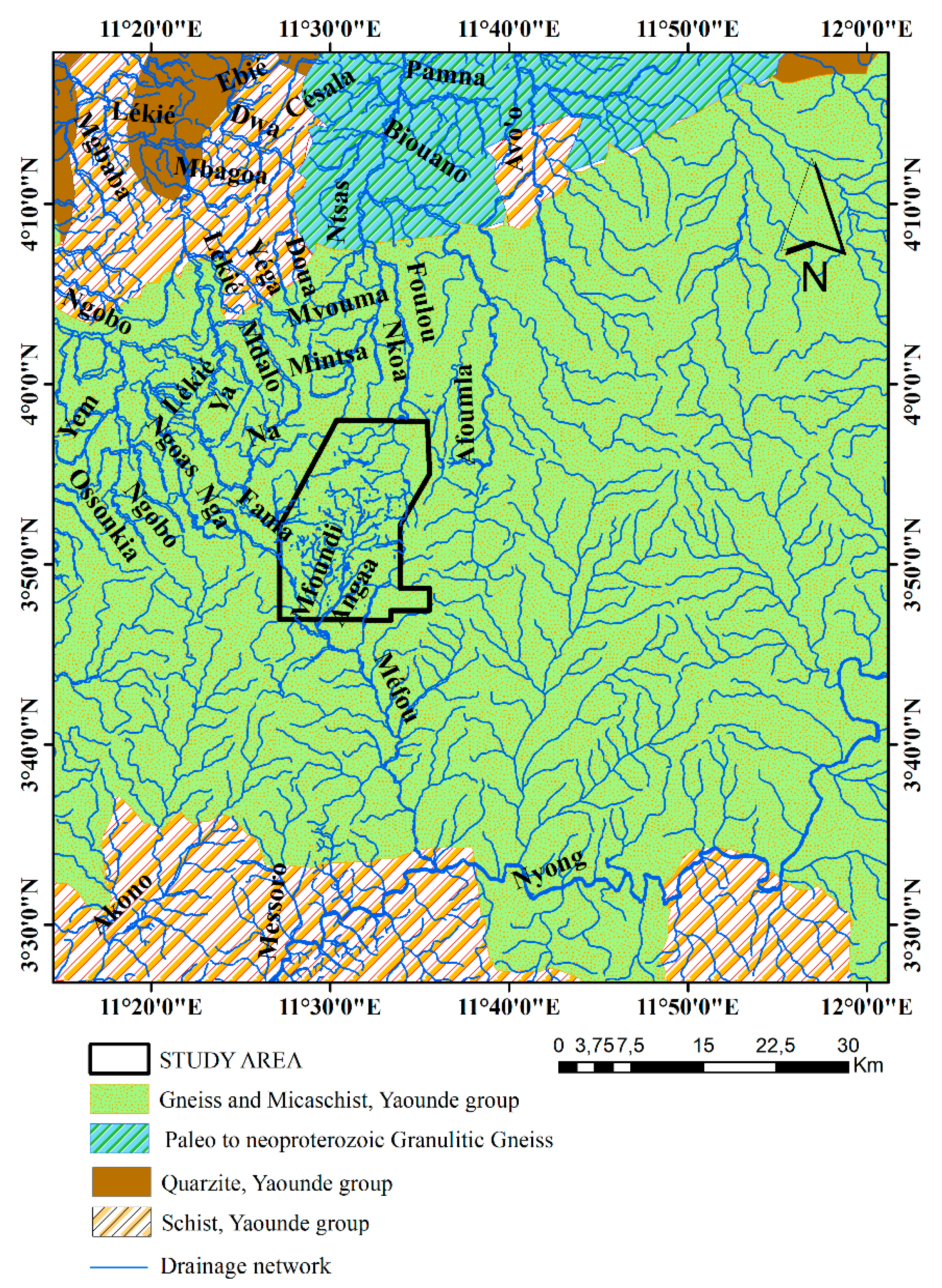
Figure 3.
Geomorphological map.
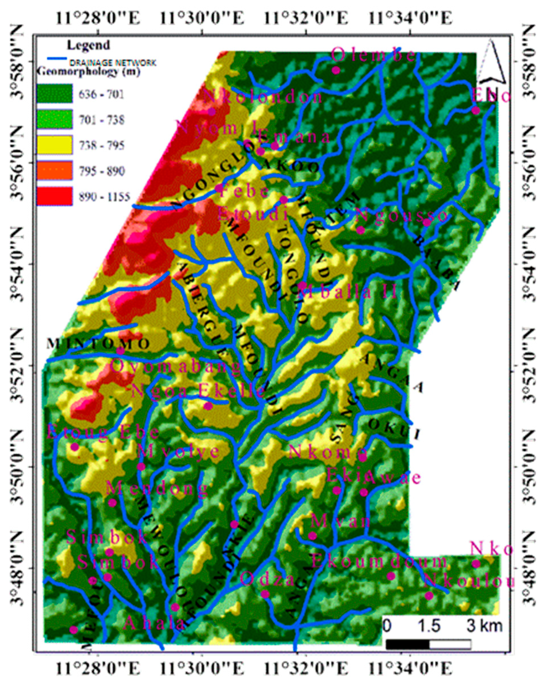
Figure 4.
Land use map.
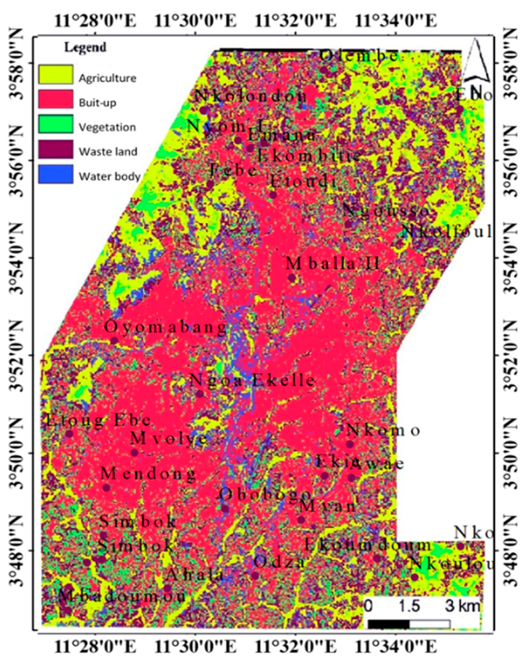
Figure 5.
Density of lineaments.
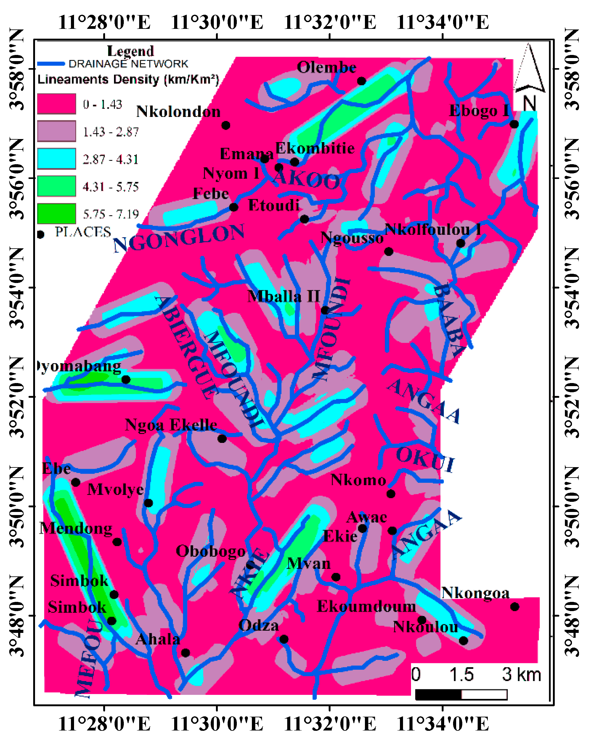
Figure 6.
Drainage density map.
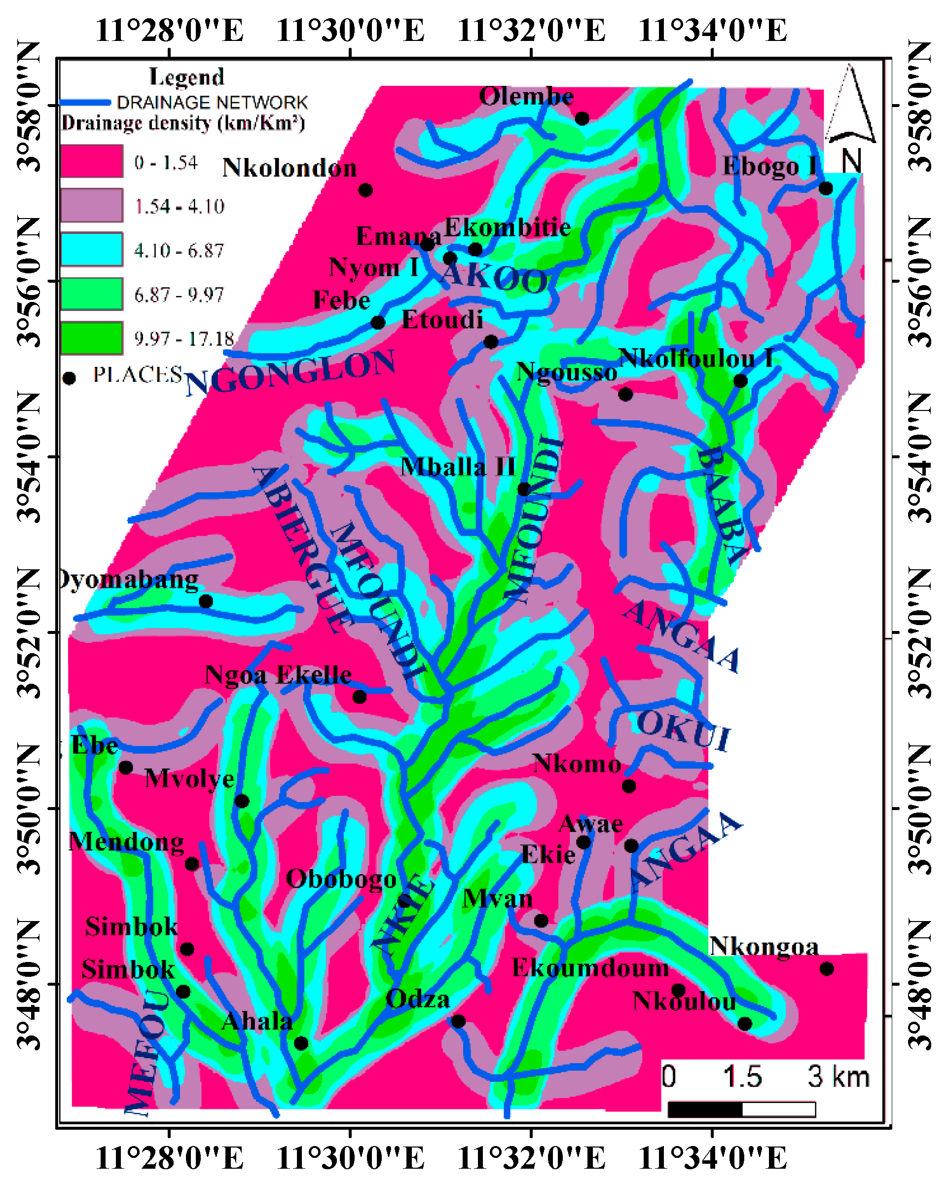
Figure 7.
Slope map.
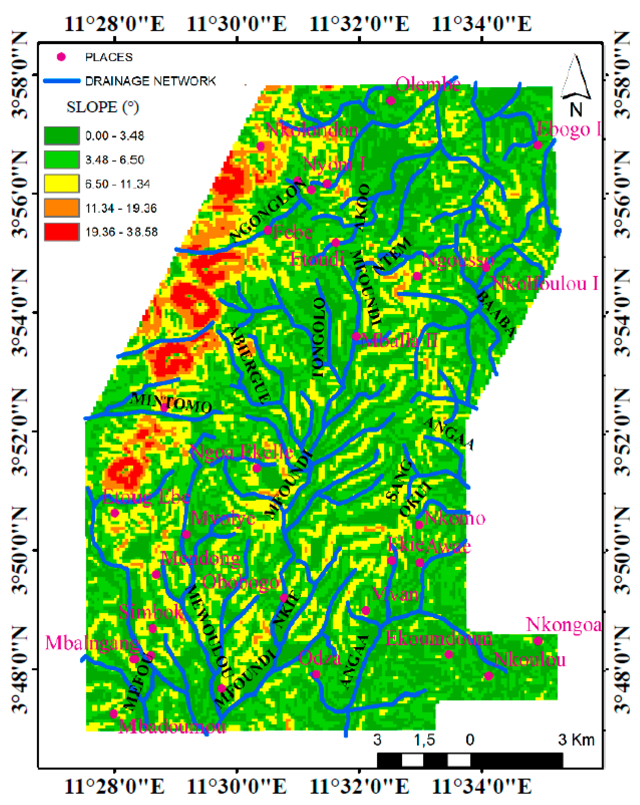
Figure 8.
Diagram for identifying aquifer zones.
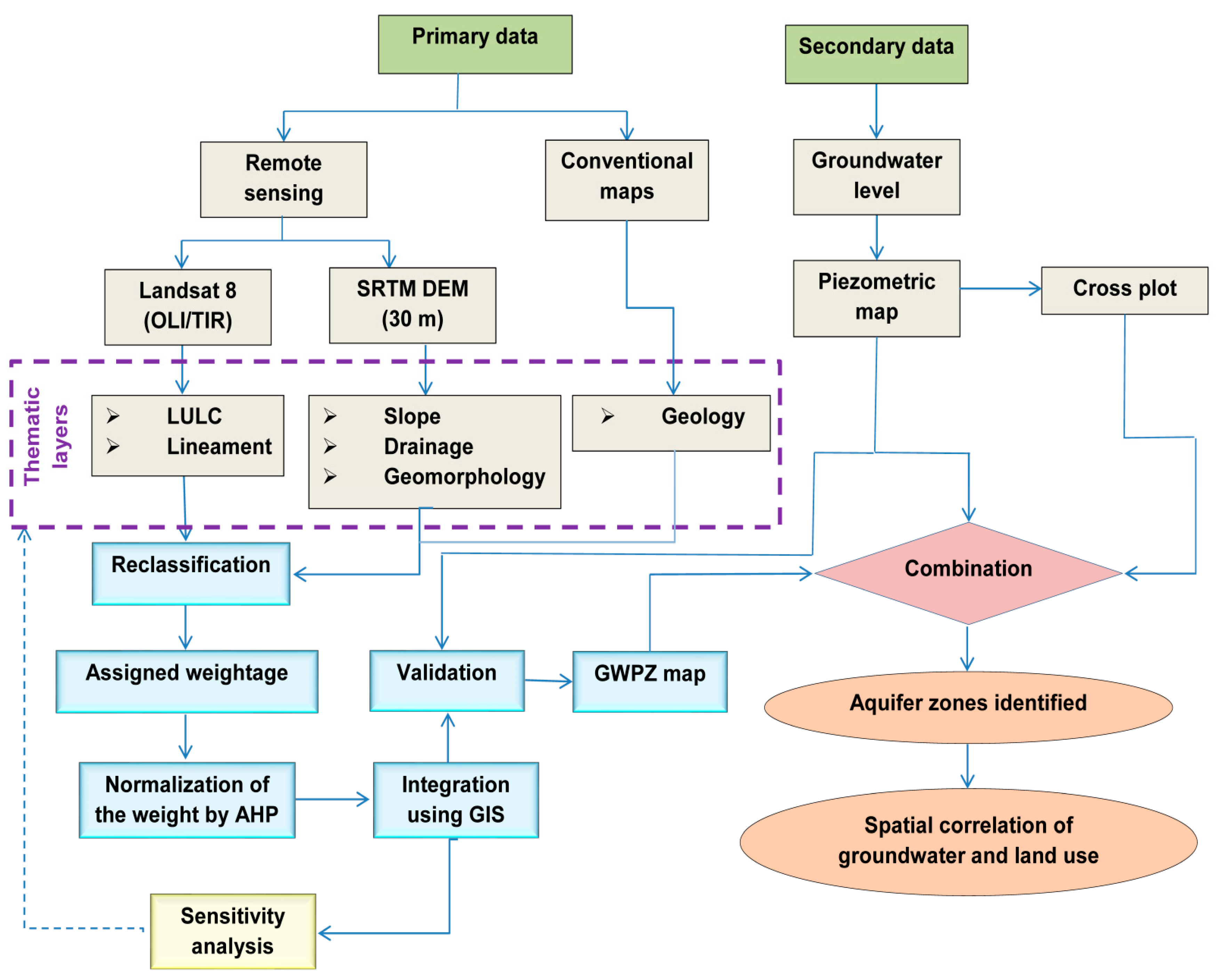
Figure 9.
hyper-sphere of correlations.
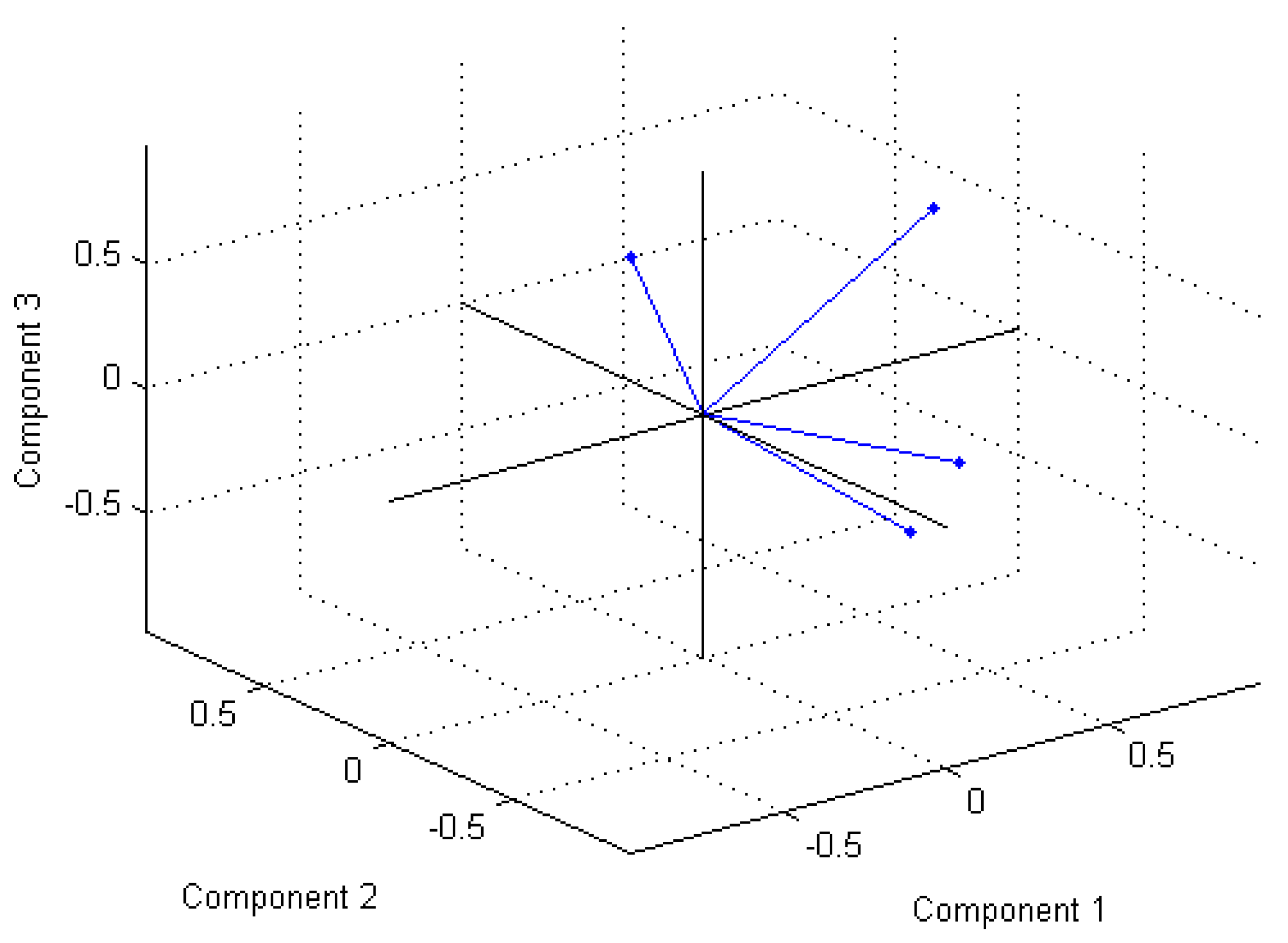
Figure 10.
GWPZ map.
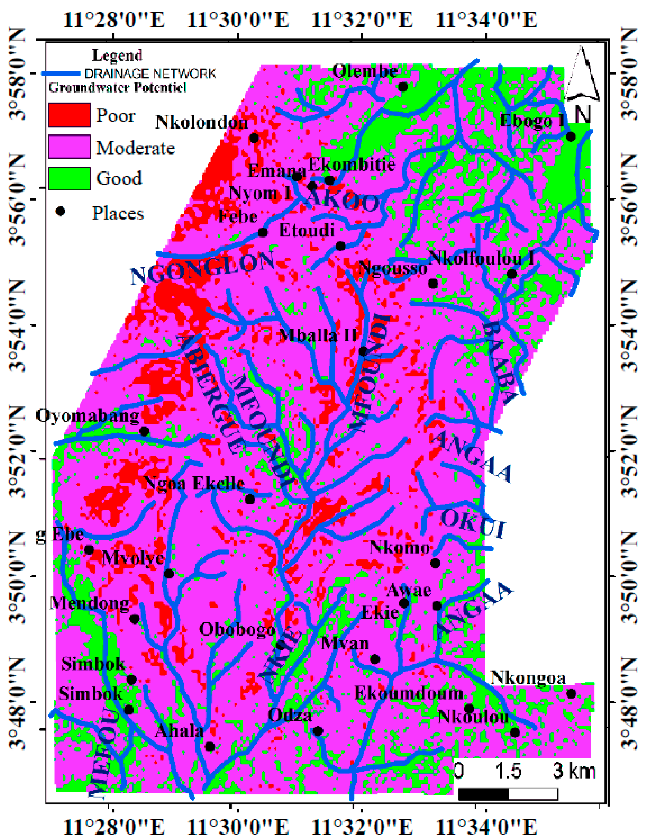
Figure 11.
Spatial distribution of GWPZ.
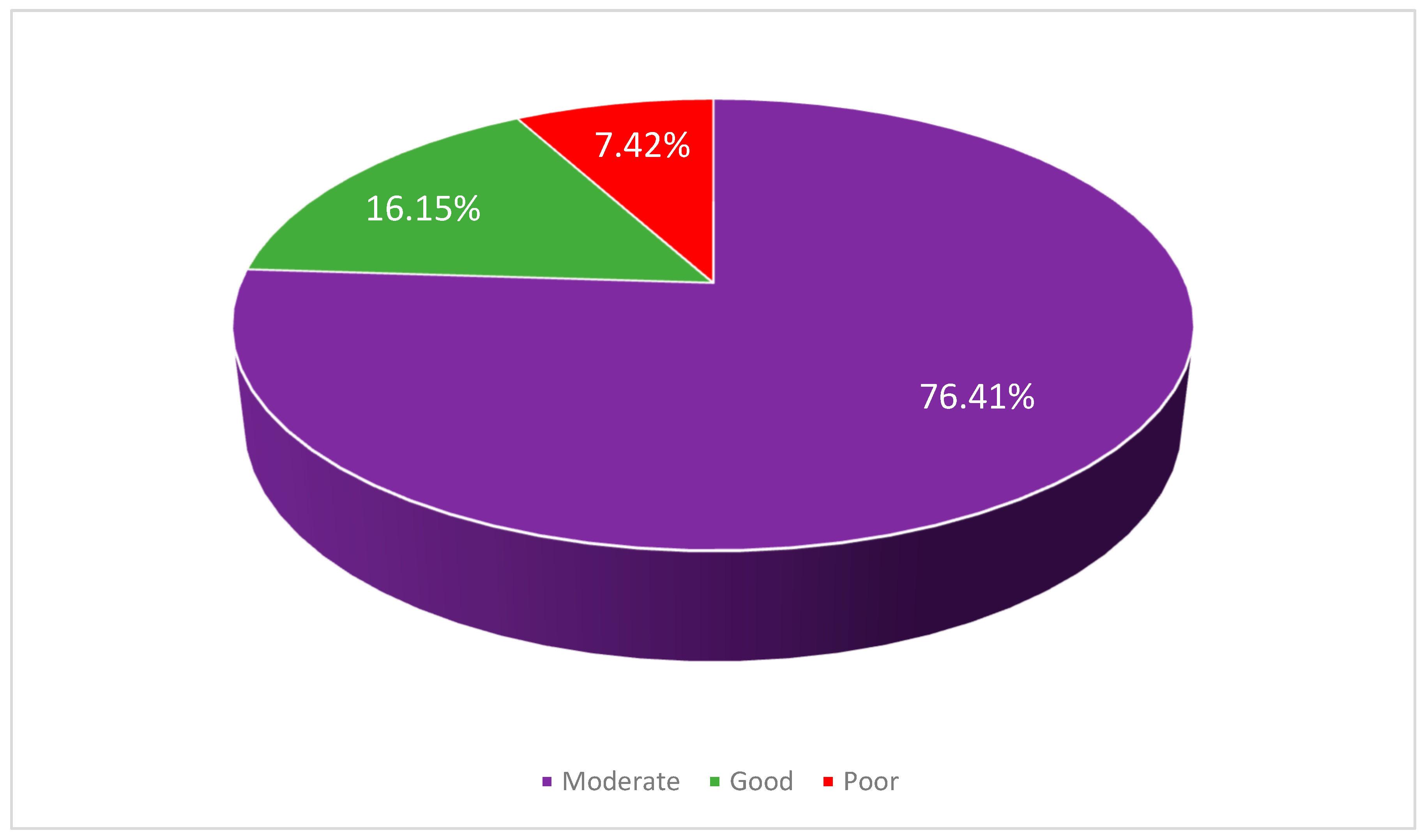
Figure 12.
Piezometric map.
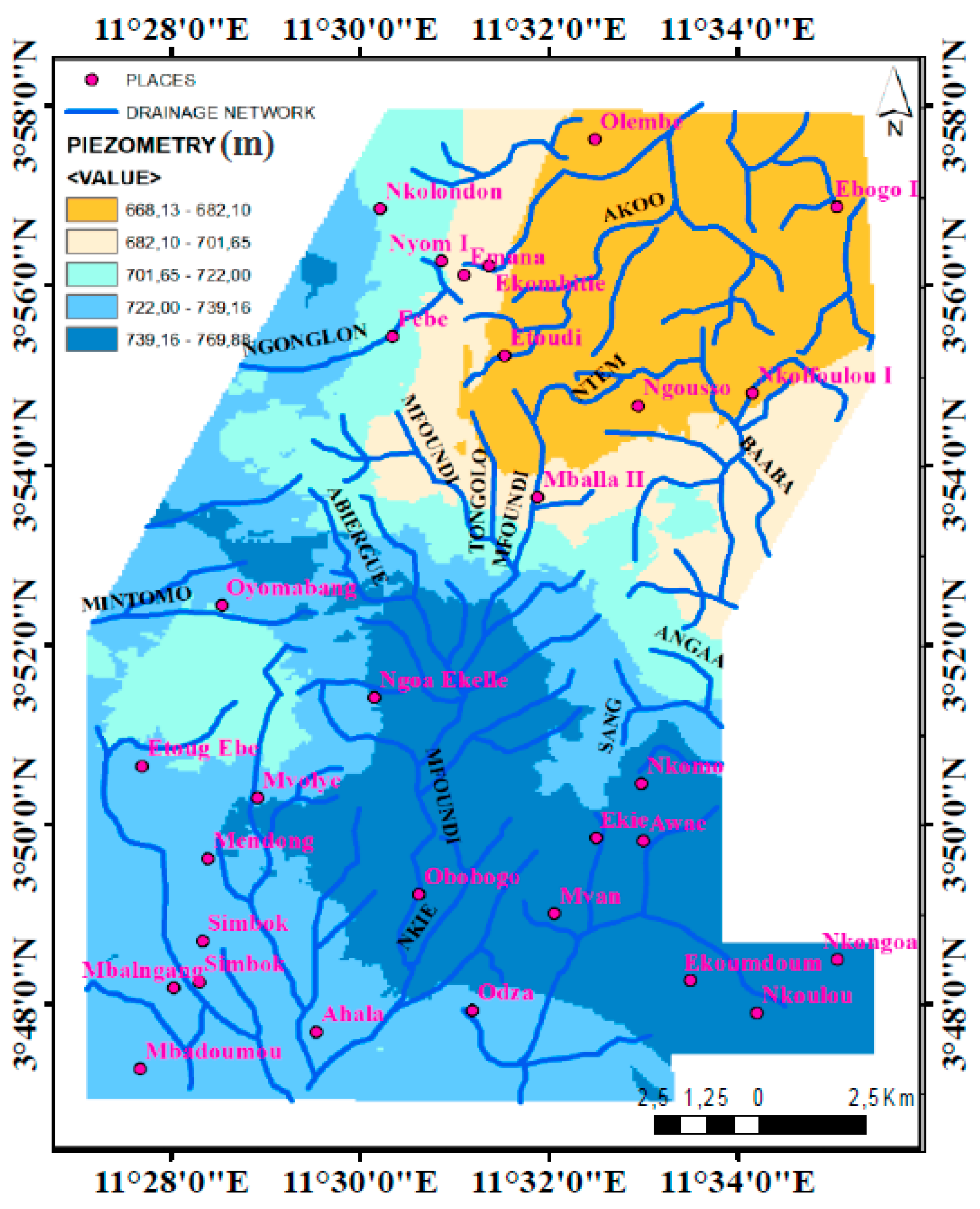
Figure 13.
Cluster dendrogram of piezometric levels.
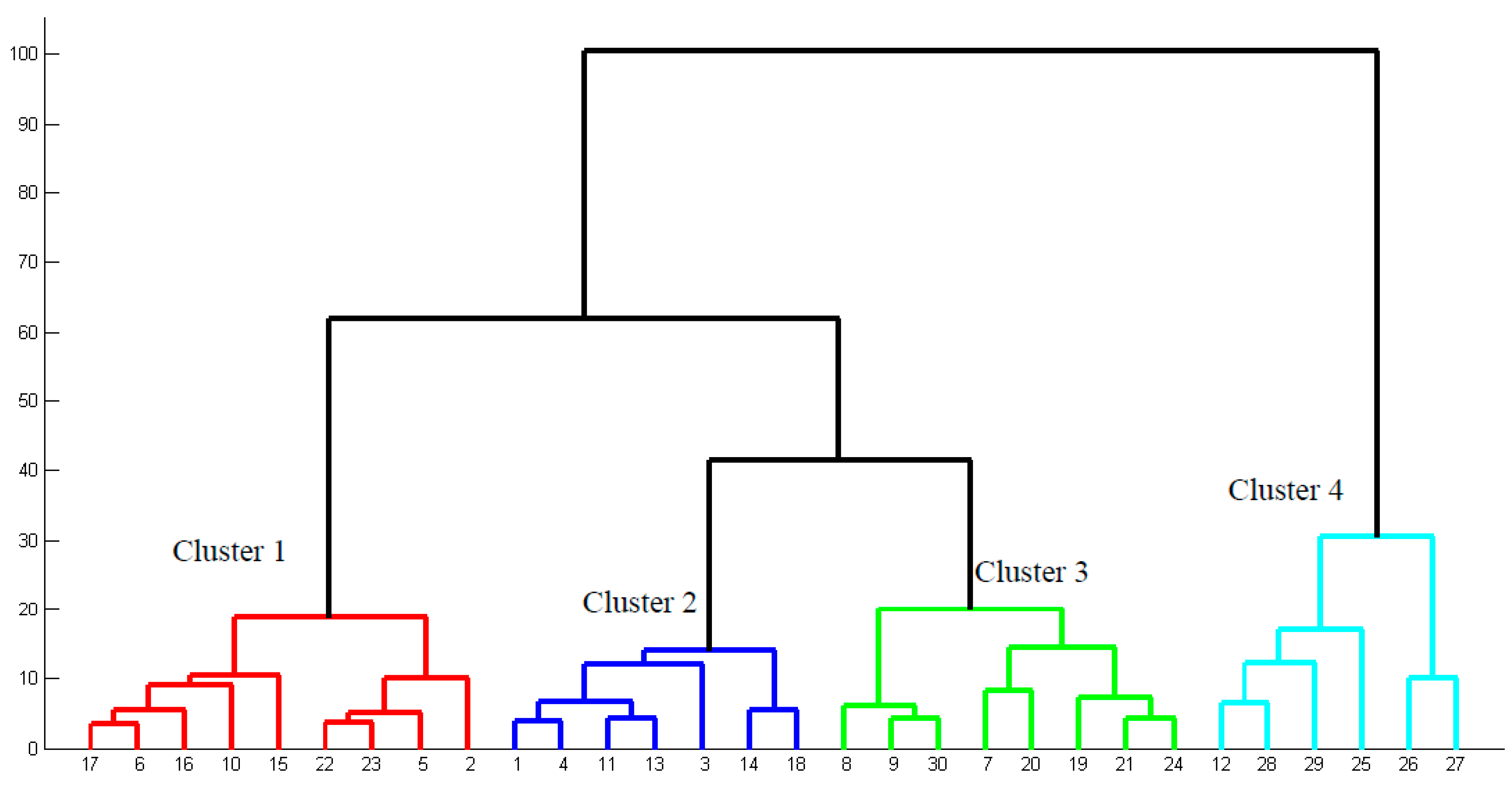
Figure 14.
Aquifer zones identified.
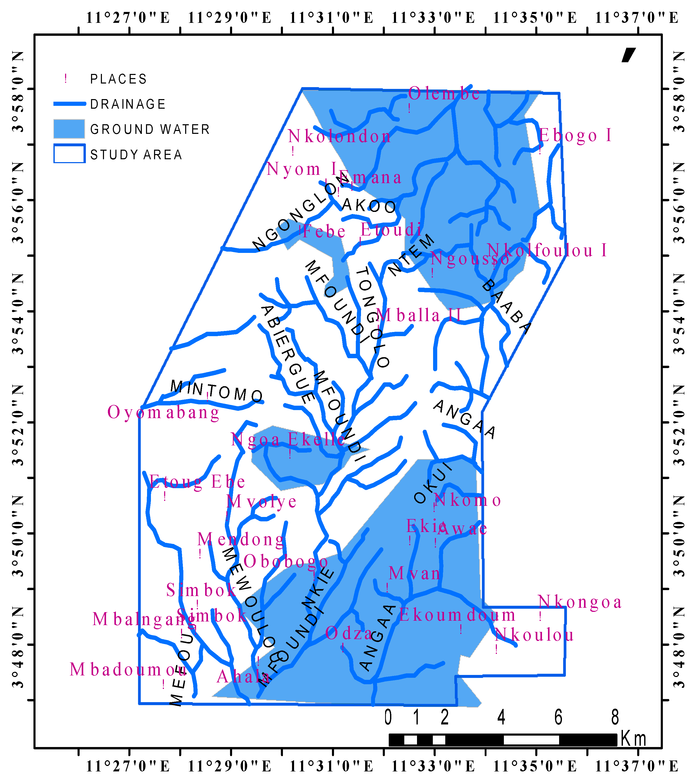
Figure 15.
Distribution of aquifers in the study area.
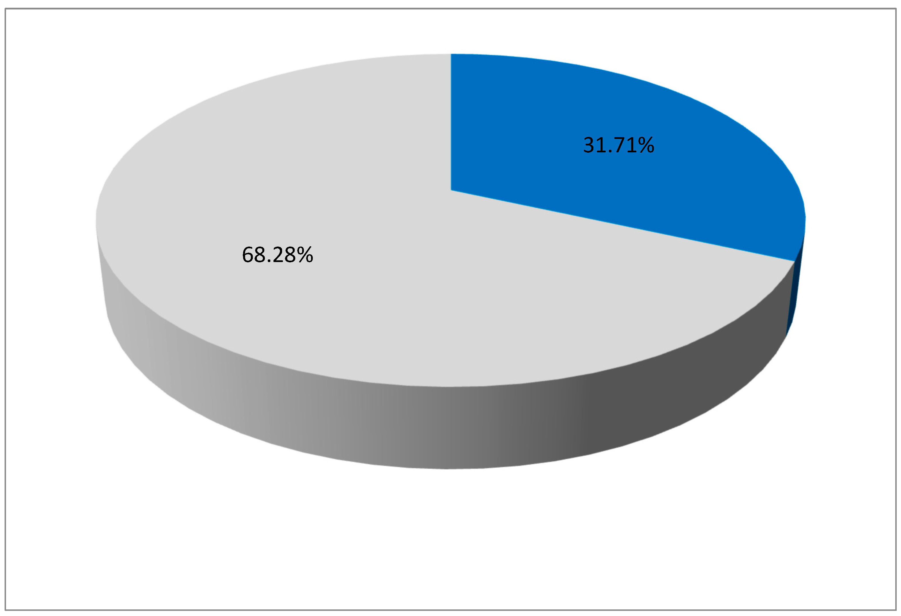
Figure 16.
Aquifer zones overlayed on land use.
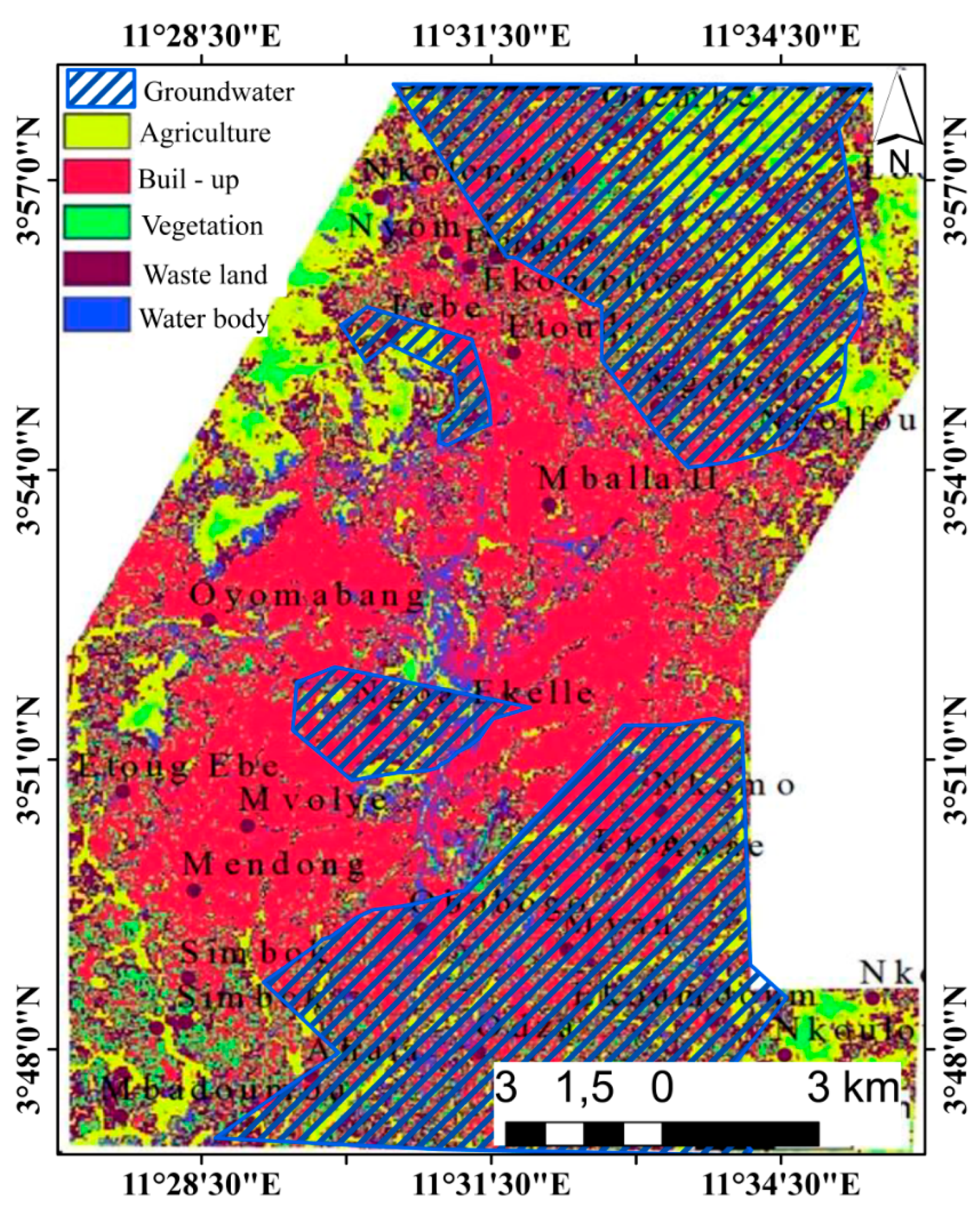

Table 1.
Classes of geomorphology.
| Elevation (m) | Area (km2) | Percentage (%) |
|---|---|---|
| 890 -1155 | 4.98 | 1.97 |
| 795-890 | 11.06 | 4.38 |
| 738-795 | 55.51 | 21.99 |
| 701-738 | 80.72 | 31.98 |
| 636-701 | 7.50 | 2.97 |
Table 2.
LULC.
| LULC | Area (km2) | Percentage (%) |
|---|---|---|
| Water body | 19.8 | 7.84 |
| Vegetation | 28 | 11.09 |
| Waste land | 62.7 | 24.84 |
| Agriculture | 20.13 | 7.97 |
| Built-up | 121.76 | 48.24 |
Table 3.
Different classes of lineament density.
| Lineament density (km/km2) | Area (km2) | Percentage (%) |
|---|---|---|
| 5.75-7.19 | 1.81 | 0.71 |
| 4.31-5.75 | 8.28 | 3.25 |
| 2.87-4.31 | 21.43 | 8.40 |
| 1.43-2.87 | 68.05 | 26.69 |
| 0-1.43 | 155.39 | 60.95 |
Table 4.
different classes of drainage density.
| Drainage density (km/km2) | Area (km2) | Percentage (%) |
|---|---|---|
| 0-1.54 | 115.27 | 45.67 |
| 1.54-4.10 | 45.67 | 22.56 |
| 4.10-6.87 | 37.00 | 14.66 |
| 6.87-9.97 | 29.76 | 11.79 |
| 9.97-17.18 | 13.39 | 5.30 |
Table 5.
different classes of slopes.
| Slope (in degree) | Area (km2) | Percentage (%) |
|---|---|---|
| 19.36-38.58 | 4.78 | 1.89 |
| 11.34-19.36 | 10.17 | 4.03 |
| 6.50-11.34 | 46.31 | 18.35 |
| 3.48-6.50 | 110.73 | 43.87 |
| 0.00-3.48 | 80.37 | 31.84 |
| Intensity of Importance | Definition |
|---|---|
| 1 | Equal Importance |
| 2 | Equal to moderate importance |
| 3 | Moderate importance |
| 4 | Moderate to strong importance |
| 5 | Strong importance |
| 6 | Strong to very strong importance |
| 7 | Very strong importance |
| 8 | Very to extremely strong importance |
| 9 | Extreme importance |
Table 7.
pair-wise comparison matrix.
| Geology | Geomorphology | LULC | Lineament density | Drainage density | Slope | |
| Geology | 1.00 | 2.00 | 3.00 | 4.00 | 4.00 | 6.00 |
| Geomorphology | 0.50 | 1.00 | 2.00 | 3.00 | 3.00 | 5.00 |
| LULC | 0.33 | 0.50 | 1.00 | 2.00 | 3.00 | 5.00 |
| Lineament density | 0.25 | 0.33 | 0.5 | 1.00 | 2.00 | 3.00 |
| Drainage density | 0.25 | 0.33 | 0.33 | 0.50 | 1.00 | 2.00 |
| Slope | 0.16 | 0.20 | 0.20 | 0.33 | 0.50 | 1.00 |
Table 8.
normalised pair-wise matrix.
| Geology | Geomorphology | LULC | Lineamentdensity | Drainagedensity | Slope | |
| Geology | 0.40 | 0.46 | 0.43 | 0.37 | 0.30 | 0.27 |
| Geomorphology | 0.20 | 0.23 | 0.28 | 0.28 | 0.22 | 0.22 |
| LULC | 0.13 | 0.11 | 0.14 | 0.18 | 0.22 | 0.23 |
| Lineament density | 0.10 | 0.08 | 0.07 | 0.09 | 0.15 | 0.14 |
| Drainage density | 0,1 | 0.08 | 0.05 | 0.05 | 0.07 | 0.09 |
| Slope | 0.07 | 0.05 | 0.03 | 0.03 | 0.04 | 0.05 |
Table 9.
Distribution of the different weights.
| S.no. | Influence factor | Classes | potentiality | Criterion weight | Rank | Normalised weight |
| 1 | geology | Gneiss | Poor | 2.00 | 0.37 | |
| 2 | Geomorphology | 636-701 m 701-738 m 738-795 m 795-890 m 890-1155 m |
Very good Good Very poor Very poor Very poor |
0.35 0.25 0.2 0.15 0.05 |
5.00 4.00 1.00 1.00 1.00 |
0.24 |
| 3 | LULC | Water bodies Built-up Wasteland Forest Agricultural Land |
Very good Very poor Poor Moderate Good |
0.47 0.3 0.125 0.08 0.025 |
5.00 1.00 2.00 3.00 4.00 |
0.17 |
| 4 | Lineament density (km/km2) | 0-1.43 1.43-2.87 2.87-4.31 4.31-5.75 5.75-7.19 |
Very poor Poor Moderate Good Very good |
0.01 0.19 0.23 0.27 0.3 |
1.00 2.00 3.00 4.00 5.00 |
0.10 |
| 5 | Drainage density (km/km2) | 0-1.54 1.54-4.10 4.10-6.87 6.87-9.97 9.97-17.18 |
Very good Good Moderate Poor Very poor |
0.34 0.23 0.16 0.15 0.12 |
5.00 4.00 3.00 2.00 1.00 |
0.07 |
| 6 | Slope (°) | 0.00-3.448 3.48-6.50 6.50-11.34 11.34-19.36 19.36-38.58 |
Very good Good Moderate Poor Very poor |
0.5 0.3 0.12 0.05 0.03 |
5.00 4.00 3.00 2.00 1.00 |
0.04 |
Table 10.
Correlation matrix.
| Longitudes | Latitudes | Piezometry | GWPI | |
| Longitudes | 1 | 0.6 | 0.8 | 0.7 |
| Latitudes | 0.6 | 1 | 0.62 | 0.66 |
| Piezometry | 0.8 | 0.62 | 1 | 0.9 |
| GWPI | 0.7 | 0.66 | 0.9 | 1 |
Table 11.
Correlation between variables and factors.
| Factors | |||||
| 3.15 | 0.46 | 0.31 | 0.08 | ||
| Variables | Longitudes | -0.49 | 0.28 | 0.78 | 0.25 |
| Latitudes | -0.45 | -0.89 | 0.06 | -0.1 | |
| Piezometry | -0.53 | 0.34 | -0.22 | -0.75 | |
| GWPI | -0.52 | 0.16 | -0.16 | 0.61 | |
Table 12.
Different classes of GWP.
| GWP | Area (km2) | Percentage (%) |
|---|---|---|
| Poor | 18.74 | 7.42 |
| Moderate | 192.86 | 76.41 |
| Good | 40.77 | 16.15 |
Table 13.
Different piezometric classes.
| Piezometry (m) | Area (km2) | Percentage (%) |
|---|---|---|
| 668.13-682.10 | 45.67 | 18.09 |
| 682.10-701.65 | 28.71 | 11.37 |
| 701.65-722.00 | 35.53 | 14.07 |
| 722.00-739.16 | 80.26 | 31.80 |
| 739.16-769.88 | 62.20 | 24.64 |
Table 14.
Integrating clusters, piezometry and potentials.
| Groundwater zone | Area (km2) | Percentage (%) |
|---|---|---|
| Groundwater | 80.85 | 31.71 |
| Hollow | 174.09 | 68.28 |
Disclaimer/Publisher’s Note: The statements, opinions and data contained in all publications are solely those of the individual author(s) and contributor(s) and not of MDPI and/or the editor(s). MDPI and/or the editor(s) disclaim responsibility for any injury to people or property resulting from any ideas, methods, instructions or products referred to in the content. |
© 2025 by the authors. Licensee MDPI, Basel, Switzerland. This article is an open access article distributed under the terms and conditions of the Creative Commons Attribution (CC BY) license (http://creativecommons.org/licenses/by/4.0/).
Copyright: This open access article is published under a Creative Commons CC BY 4.0 license, which permit the free download, distribution, and reuse, provided that the author and preprint are cited in any reuse.


