
Submitted:
06 February 2025
Posted:
08 February 2025
You are already at the latest version
Abstract
To the best of our knowledge, we define a new IoT-Osmotic simulator supporting 6G infrastructures, leveraging the similarities in Software Defined Wide Area Network (SD-WAN) architectures when used in Osmotic architectures and User-Centric Cell-Free mMIMO architectures - one of the proposed solutions for 6G infrastructures. As part of this work, we showcase the possibility of integrating SimulatorOrchestrator with a patient digital twin generating patient healthcare data, such as vital signs and emergency alerts, in smart ambulances, thus generating additional IoT streams of data, thus contextualising the approach within the healthcare domain, while showcasing the possibility of orchestrating different simulators at the same time. The combined provision of these two aspects joined with the addition of a ring network connecting all the first-mile edge nodes (i.e. Access Points) enables the definition of new packet routing algorithms streamlining previous solutions from SD-WAN architectures, thus remarking both the benefit of 6G architectures in achieving better network load balancing, as well as showcasing the limitations of previous approaches.
Keywords:
IoT
; Healthcare transportation
; 6G Architecture
; Traffic Simulators
; Patient Monitoring
1. Introduction
The healthcare sector exploits Internet of Things (IoT) technologies to improve both patient care and health outcomes by leveraging the basics of Smart City infrastructures [1,2]: by equipping ambulances with IoT sensors to transmit patients’ condition from ambulances to hospitals to allow for medical staff at the hospitals to determine and prepare any necessary patient treatment in advance of ambulance arrivals, saving valuable time [3,4,5]. Ramesha et al. [6] extend this by connecting ambulances to traffic control units for uninterruptedly routing the ambulances through synchronised traffic lights, which might be turned green alongside the route to the hospital – thereby reducing the time needed to get patients to the hospitals. Given the time-sensitive nature of ambulances rushing patients to hospitals, it is equally essential that the patient data is transmitted from the IoT-equipped ambulances to the hospitals as quickly as possible to give as much time as possible to the medical staff at the hospitals to prepare for incoming patients adequately. Due to the mobile nature of ambulances, the straight transmission of data from the ambulances to the hospitals is likely to be unstable due to unpredictable environmental obstacles, high vehicle speeds and traffic congestion. These issues lead to highly dynamic network topologies, requiring road-side units (RSUs) as edge nodes to ensure a constant, stable network connection for the ambulances. RSUs, planted across an environment, can collect patient data from nearby ambulances and forward it to the relevant hospitals for processing. In e-health applications, particularly during emergency medical transportation, the Quality of Service (QoS) requirements are stringent, with a necessity for low-latency and high-reliability communication channels. This ensures that patient data transmitted from IoT-enabled ambulances to hospitals is received without delay or loss, enabling timely medical interventions [7]. To ensure the effectiveness of IoT systems in real-world settings, researchers have stressed the importance of accurately modelling and simulating such systems [8].
As more patient data will be streamed and collected within smart cities [9] thus including real-time data collected from patients’ wearable devices [10] while at home, this extremely interconnected scenario will severely increase the amount of internet traffic within the Osmotic infrastructure, the network infrastructure in place must handle the data transfer and processing of the transmitted information in real-time, where both mobile and static IoT devices coexist. In the context of such healthcare transportation research, advanced simulation platforms are critical to evaluating and improving patient transportation strategies, including testing the necessary network infrastructure. Despite the importance of trace data for network simulators, there is limited public availability [11,12,13], which has led to the generation of traces either from real-world traffic data or, in some cases, synthetic traces generated using simulators. However, this comes with the trade-off of a lack of realism. This research extends SimulatorBridger [14] into SimulatorOrchestrator (https://github.com/LogDS/SimulatorBridger/releases/tag/v1.0, Accessed on the 18th of January, 2025) to allow for the direct ingestion of real-time communication events coming from another simulator external to the VANET, while also considering possible minimal extensions of the simulator enabling a 6G infrastructure via Cell-Free networks. As a use case of the former, we consider patients Digital Twins generating traffic to update clinicians via the Cloud in real-time on the health conditions of the patient recovering at home. This is an important step, as it showcases the possibility of extending this simulator to a general-purpose orchestrator of different simulators contextually generating events of interest.
As with [1], the UK’s new NHS electric vehicle initiative to help reduce its carbon footprint [15] was a driving force behind choosing the healthcare sector for the simulated use case of SimulatorOrchestrator. As a result of these advancements, our previous work related to SimulatorBridger [1] was extended to handle patient health information transmitted by IoT devices during the transport process and accurately simulate scenarios in which (EAs) are used to transport patients whilst ensuring the timely and secure transmission of health data. This motivates our extension of the former to support patient IoT data beyond vehicular patterns further: in the present paper, we extend the former solution also to include new communication events that might be while also including data that can be streamed in real-time by home patient care requiring ad hoc monitoring. This is particularly crucial in e-health scenarios where QoS must be guaranteed to avoid delays or data loss that could adversely affect patient outcomes. The addition of an external patient simulator required us to extend the simulator further to address the possibility of making multiple simulators interact and be orchestrated to simulate one single scenario of interest. This required a major architectural restructuring of the initial work, thus leading to a novel simulator, named SimulatorOrchestrator (See RQ №2..)
From the communication architecture perspective of a 5G network supporting SD-WAN Osmotic infrastructure, this paper addresses the main limitation of our previous work [1]. The choice of MEL allocation policy originally had no impact on network behaviour. If a communication was from a device near a busy edge node with bottlenecked MELs, it had to be processed by one of those bottlenecked MELs. If all the MELs were bottlenecked, then not only was there not an impact shown in the results in [1], but no impact should be expected. By leveraging the 6G architecture and by assuming that all the first-mile edge nodes (APs being RSUs) are connected in a MAN token ring network, we aim to load balance the transmission of packages better: we can avoid bottlenecking by re-forwarding the packet to a “quieter” edge subnetwork, i.e. a network having less traffic allocation (Figure 1). Our paper shows the effectiveness of exploiting the Million Instruction Per Second (MIPS) allocated to each MicroELement (MEL) component supporting the packet transmission (Section 3.1.3).
The paper addresses the following research questions:
- RQ №1.
- It is possible to minimally extend an Osmotic Simulator also to support 6G Cell-Free Architecture: after observing that (i) both can operate on software-defined networks (SDN) [16,17], (ii) there exists a parallelism between Edge nodes associated with computing abilities (Section 2.2) [18] and the UC CF-mMIMO Access Points (AP) (Section 2.1), (iii) the parallelism between osmotic Central Agents [14,18] and cell-free Central Processing Units [19,20,21], and (iv) given that SimulatorOrchestrator supports all of the aforementioned osmotic architecture features via SimulatorBridger [14], then our previous simulator SimulatorBridger can be minimally extended also to simulate cell-free architectures (Figure 3). By assuming almost simultaneous communication across the Edge nodes belonging to the same metropolitan area network (MAN) through a Gigabit Token Ring (Section 3.1.3), it is possible to establish connections across different area networks, thus breaking the rigid cell and edge network structure.
- RQ №2.
- It is possible to orchestrate a network simulator with another one providing additional packet transmission events to the former: by extending the interface of our previous simulator, SimulatorBridger, to run only within subsequent time intervals (Section 3) and by allowing the possibility of pause for then resuming the simulation, it is possible to concurrently run it alongside other simulators generating potential new packet transmission events (Figure 3). In this paper, we take into consideration patient digital twins transmitting healthcare data to the cloud (Section 3.1.2) running on a pre-initiated MQTT protocol (Section 2.3), and separated from VANET or Connection Counting [22] inputs for vehicular traffic (Section 3.1.1).
- RQ №3.
- The combined provision of SD-WAN and Cell-Free architectures enables efficient packet routing algorithms ensuring QoS: given the fulfilment of RQ №1., we propose a new MEL allocation policy crossing the boundaries of a single Edge network (Section 4.3) which, when combined with our previously-introduced MCFR algorithm (Section 4,23]), effectively reduces the number of active communications while increasing the packet rate (Section 5): this solution outperforms routing algorithms working on a 5G architecture not working on a Cell-Free assumption. This is achieved by centralising the execution of the routing algorithm at the Central Agent/Central Processing Unit level rather than at the single Edge gateway as in [17], thus allowing the re-route of each packet to be sent to the cloud via a specific “quiet” (e.g., non-busy) network. Preliminary results suggest that such an algorithm.
We investigate this by generating realistic traffic patterns expressed as mobility traces (MTs) through SUMO. We choose to consider those occurring in Bologna (https://github.com/DLR-TS/sumo-scenarios/tree/main/bologna/acosta, Accessed on the 18th of January, 2025), a renowned healthcare Smart City [9], which was extended by placing 3 patients at 15 of the 16 edge nodes in the smart environment: one low risk of health problems, one medium risk and one high risk. At the final edge node, we placed 15 patients, 5 at each risk level, to model a hospital with patients at different recovery levels. Patients transmit their health data towards the cloud via the edge every 10s, until they become high risk, at which point they increase the transmission rate to every 1s. This increased transmission rate aims to help provide healthcare professionals with the most up-to-date information required to treat patients with a high risk of negative health consequences.
2. Related Works
2.1. 6G Architecture
Recent work [24] highlights the potential of 6G in medical contexts, proposing an architecture where modular application functions (MAFs) dynamically interact with network resources, adapting their requirements based on current network conditions. This capability is especially relevant for healthcare, as it enables resource allocation adjustments in real-time to prioritize critical applications such as remote patient monitoring and emergency response.
One of the primary potential technologies for 6G is cell-free massive multi-input multi-output architecture (CF-mMIMO) [25]. The key idea behind CF-mMIMO is the distribution of access points (APs) throughout an environment to create a sizeable homogenous coverage area. This technology aims to combat issues with cell-based architectures, including inter-cell interference and signal degradation as a device gets further away from the cell centres [26,27]. An initial assumption within CF-MIMO systems was that all devices should be able to access all APs to overcome user performance and location-based issues. However, this results in problems scaling as the number of connecting devices grows, such as high computational complexity and high power consumption. To tackle this scalability issue, the user-centric CF-mMIMO (UC CF-mMIMO) has been proposed, where devices now need only connect with a smaller number of nearby APs. UC CF-mMIMO tackles the scaling issues while maintaining consistent coverage for all devices within the networked area [26].
Within cell-free based environments, the APs are connected to a central processing unit (CPU) which receives the data via the APs and processes all the available data [26,27,28]. To improve this architecture, mobile edge computing (MEC) technologies can be combined with the APs within a UC CF-mMIMO by equipping the APs with MEC servers, as was the case with [29] and [30]. Within the MEC UC CF-mMIMO, devices can connect to a nearby AP to transmit the data; the data can then be processed/preprocessed before being transmitted towards a central server/processing unit. Through the incorporation of MEC servers with the APs networks get the combined benefits of cell-free based technologies tackling problems with signal degradation and inter-cell interference with the benefits of MEC computing, which help tackle the ’critical latency requirements of computationally intensive tasks’ introduced with 5G technologies [29]. Within these MEC CF-mMIMO, the APs can remain connected to the CPUs via reliable front-haul or back-haul links, either wired or wireless, depending on what best suits both the network topology and environmental topology. [21,29]. Within UC CF-mMIMO, a cluster of APs can be assigned to a single MEC server, and therefore, it is also possible to have multiple MEC servers, each with a cluster of APs. It is then important for the MEC servers to be able to manage their APs correctly. This can be achieved through the use of distributed software-defined networks (SDNs) [16], as they can control the utilisation of both the MEC server resources, as well as its associated APs, through the use of software, for example, routing the incoming data towards the APs through the network towards its destination, e.g., a cloud data-centre.
Within UC CF-mMIMO it can be beneficial the efficiency of the network for all APs to be connected to a central processing unit which has perfect knowledge of the channel state information (CSI) within the network to aid with network and planning [19] coordinating the communications from the IoT devices which connect to the APs [20]. This is similar in concept to the central agent in osmotic computing [18], makes decisions on the operations performed by the other agents within the network.
By leveraging the flexibility of a cell-free network architecture in 6G, which adopts a user-centric design coupled with MEC-equipped APs/RSUs as edge nodes, we anticipate our simulator can provide seamless and high-quality connections for urban healthcare settings where smart devices rely on stable and continuous connectivity [31]. This paper aims to place the simulator at the forefront of healthcare IoT research, incorporating advanced communication frameworks that support highly responsive, data-intensive healthcare systems in smart city environments by challenging minor possible extensions and assumptions at their boundaries while determining whether those will suffice to achieve the 6G requirements.
2.2. IoT and Osmotic Simulators
IoT and Osmotic (Edge/Cloud) simulators are currently used to simulate network traffic conditions under different network and resource allocation policies for streamlining real-time communications [32]. As a compromise from modelling and simulating complex communication patterns over many devices, simulators such as [23,33] do not fully simulate all 7 OSI layers while focusing on the most relevant ones. This constraint is born of necessity due to the vast range of requirements and protocols found across disparate IoT devices, adding additional complexity to any simulation aiming to comprehensively simulate any, let alone all, of the OSI layers. Concerning the IoT and Osmotic simulator presented in the current paper, the Presentation and Session layers simulation took between 1 hour 30 minutes and 2 hours and 30 minutes real-time to simulate just 300 seconds (5 minutes). Given this disparity, it would have been impractical to attempt the simulation of all OSI layers, even if it would have led to a more realistic network and a more complete simulation. However, aside from simply losing increased realism, not simulating the full OSI stack comes at the expense of lacking any information which may be necessary for simulating cybersecurity-related VANET scenarios, such as battery-draining attacks [34]. VANETs are highly susceptible to network security breaches, impacting road congestion and public safety [35]. Furthermore, each OSI layer has its vulnerabilities, meaning for the current state-of-the-art to accurately determine how susceptible a given network topology is to attacks, all OSI layers would need to be simulated [36]. Such scenarios are outside the scope of this work, and so focusing on the Session and Presentation layers was deemed to be sufficient for this work, as our major interest is to determine how network infrastructure and specific network routing policies might drastically affect the communication delays within Smart City scenarios. Last, to the best of our knowledge, no IoT and Osmotic simulator was currently extended to also support 6G architectures.
2.3. MQTT Protocol
The MQTT publish-subscribe model is identified as a suitable real-time monitoring solution, particularly effective for mobile healthcare applications like ambulances and dynamically changing vehicular networks. This lightweight protocol ensures efficient data transfer with minimal delay, critical for transmitting patient data and vehicular traffic information in real-time [37]. MQTT helps streamline real-time monitoring systems by reducing bandwidth usage and improving response times, prioritizing only necessary data for immediate processing. Research on cooperative driving communications demonstrates the importance of timely data exchange for coordinated and ethical vehicle behaviours, highlighting the need for low-latency, real-time communication in similarly dynamic environments [38]. Similarly, recent studies on scalable network solutions for large UAV swarms emphasize the importance of efficient data management across adaptive networks, underscoring the value of robust algorithms to handle data flow in large-scale, fast-changing systems [39]. Given this, the simulator freely assumes that each patient and vehicle within the simulation already went through the preliminary phase of the protocol, thus only simulating the par where each IoT device (both patient and vehicle) publishes the content to the MQTT broker being distributed across the network across all the cloud virtual machines.
3. SimulatorOrchestrator for 6G CellFree Architectures
This paper postulates the possibility of achieving 6G architecture by simply extending an Osmotic architecture also to consider cell-free infrastructure and a better connection across all the nodes belonging to the Edge communication layer. To this end, we also show the need for further extending the routing policies to acknowledge the proposed network infrastructure better. To demonstrate this, we extend our Osmotic architecture from SimulatorOrchestrator, already encomassing the combination of a VANET simulator for vehicular traffic with an Osmotic architecture simulator, by also considering a patient Digital Twins generating additional packets with different levels of urgency, vehicular mobility, edge computing, and Osmotic computing in a smart city environment providing a Cell-Free infrastructure. The generator is specifically designed to handle situations in which real-time healthcare data is collected, transmitted, and processed. At the same time, patients are transported in vehicles equipped with IoT-enabled medical devices, such as electric ambulances (EAs). While Figure 2 describes the simulator from the perspective of the agents being simulated within the software infrastructure, Figure 3 describes the simulator as an orchestrator across different simulators.
Figure 2.
Agent components supported in SimulatorOrchestrator.
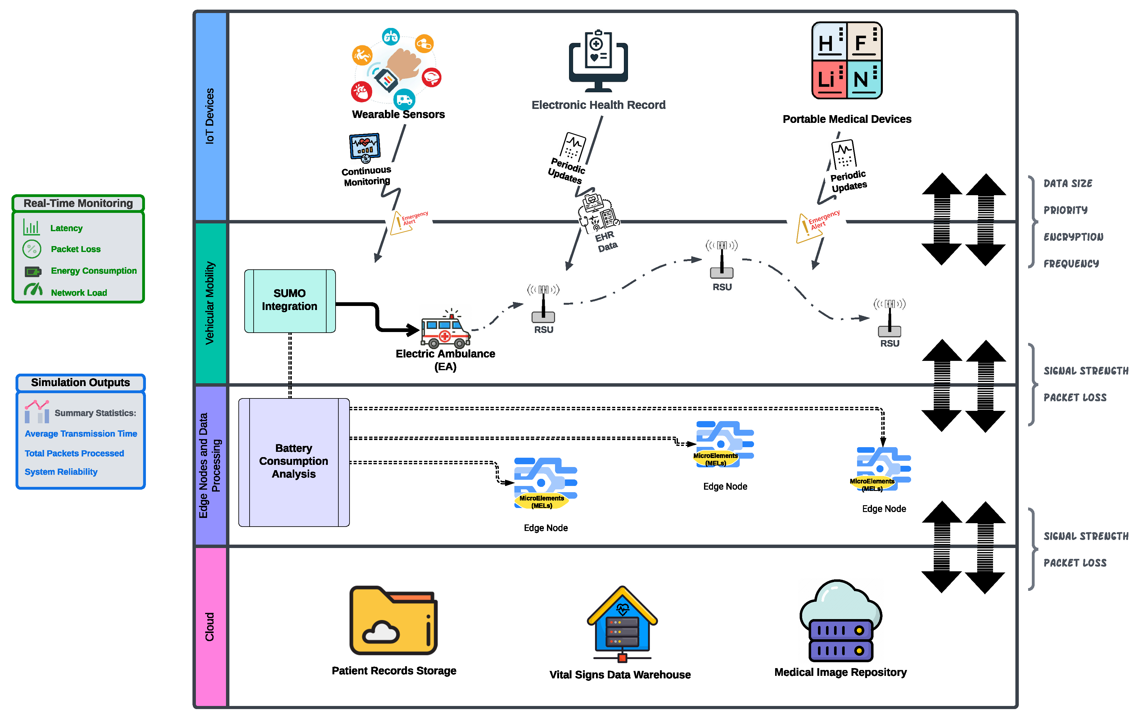
Figure 3.
Proposed Architecture for SimulatorOrchestrator: parts in blue remark extensions from previous work and ones in red reveal novel additions to the architecture.
Figure 3.
Proposed Architecture for SimulatorOrchestrator: parts in blue remark extensions from previous work and ones in red reveal novel additions to the architecture.
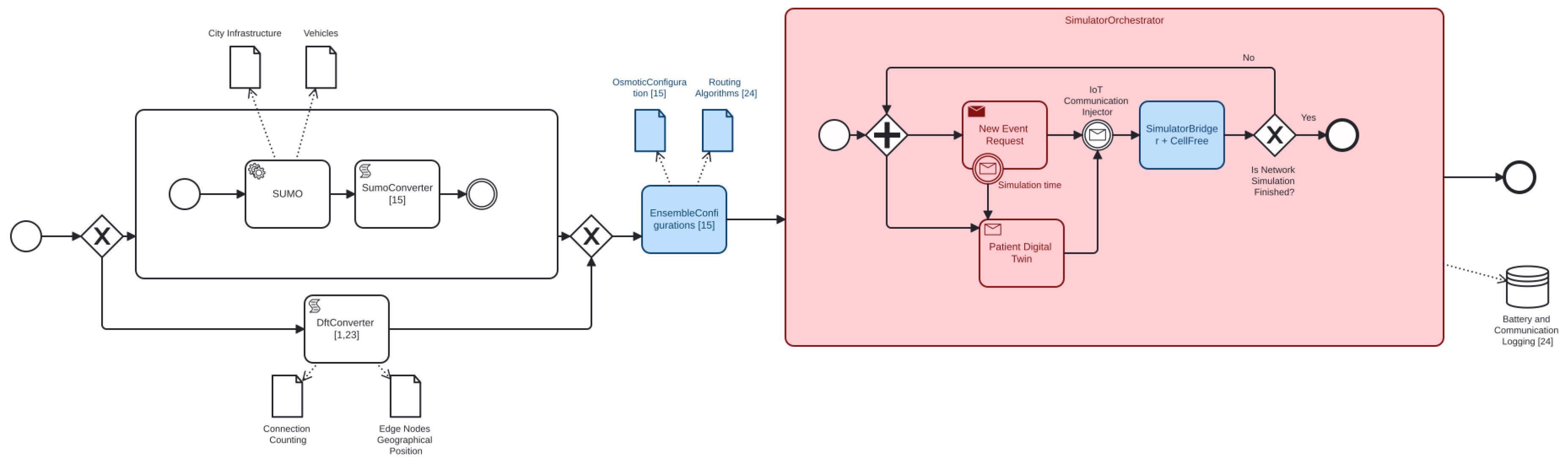
SimulatorOrchestrator procedurally generates the network infrastructure by considering either the RSU distribution within a city environment [14] or by precisely providing the exact location of their position [1,40]. Each edge subnetwork is then created from a cluster of connected components that can easily share the traffic information and constitute a single communication island completely detached from the other cells (EnsembleConfigurations). While the first configuration is the preferred choice when we possess more precise traffic vehicular information, the latter is used when we are interested in approximate IoT communications through connection counting. We consider both solutions static traffic generators, as they provide vehicular traces that cannot dynamically interact with the main simulator of choice. In particular, when running SUMO to obtain precise vehicular information, we generate precise vehicular traces per vehicle in the form of location-time-step pairs (LTSPs). This data was then stored in a SQL table [23], which will be then used by the main SimulatorBridger network communication simulator; LTSPs lead to the scheduling of ’wake-up’ simulator time events, i.e. times at which SQL data is to be injected into SimulatorBridger allowing for the positions of the vehicles to be checked and initiating any possible communication from a vehicle if near to a first-mile edge node (i.e., RSU as AP), thus reaching the nearest one [14]. This approach is only suitable for either simple situations where the results can be computed at runtime or deterministic simulators, with no dynamic behaviours, under the assumption that the cars will not change their routing algorithm depending on the possible events generated by the main networking simulator (SimulatorBridger).
However, one of the goals of SimulatorOrchestrator is the ability to combine and connect multiple simulators with the IoT simulator that would potentially need to adapt their behaviour depending on the current network status. Among those, we can also consider non-deterministic simulators relying on complex decisions that cannot simply be computed at runtime, as well as others requiring access to the current state of a different simulator to be used in their own decision-making via the database’s simulator logging the current status of the network. In such cases, it is clear that simply running each simulator before running the main Osmotic simulator and simply injecting the traces of the vehicles on the Osmotic simulator would not result in a realistic set-up. This then requires that any simulator requiring dynamic updates be run simultaneously with the main networking architecture and allow any newly generated communication initiation step to be injected in SimulatorBridger. In our case, the state of a patient’s health does not affect vehicle traffic or vice versa, so we do not need to account for how these two aspects interact, meaning we can still use the traffic simulator’s batched output. On the other hand, the network traffic from each scenario interacts and impacts the whole network, so the data from the traffic simulator and the patient health data must be injected into the IoT simulator.
The main impact of extending the previous simulator architecture so to encompass an orchestration of multiple simulators running at the same time is highlighted in red in the BPMN diagram from Figure 3: after an initialisation step, which encompasses the generation of the networking architecture from either the connection counting strategy or from a VANET simulator such as SUMO, the data resulting from this is sufficient to run the previous SimulatorBridger fully by considering vehicular updated positions via LTSP: the network simulation then finishes when there are no more networking events to be handled. When this happens, a shutdown process is started after which we collect further network statistics [18]. To allow the interaction with other simulators, SimulatorOrchestrator will require the definition of a simulation time granularity interval , after which the Osmotic simulator being SimulatorBridger is temporarily suspended. This results into an event dispatch request towards the other concurrent simulators (e.g., the Patient Digital Twins), which might generate new communication events to be injected while running SimulatorBridger occurring within the time frame of the forthcoming time intervals. When the other concurrent simulators terminate the generation of new potential communication events, the computation of SimulatorBridger is then resumed, thus continuing to handle other requests. At the time of writing, the last communication time will still be determined by the LTSP with the greatest time value, after which no further requests to the other concurrent simulators are dispatched while waiting to handle the network shutdown event.
3.1. Simulation Input
We now discuss the different kind of simulation inputs currently supported by our simulator, overall orchestrating a vehicular (Section 3.1.1) and a patient digital twin (Section 3.1.2) into the main backbone constituted by a Cell-Free Osmotic Simulator which is ready for simulating futuristic 6G Architectures before deploying them in the real world.
3.1.1. Vehicular Mobility Patterns (SUMO, Connection Counting)
When patients are transported by smart vehicles, such as electric ambulances (EAs), the data is continuously transmitted to nearby RSUs/APs/first-mile edge nodes positioned along their route. By integrating the proposed health data generator with the traffic generator, SUMO [41], the system can accurately simulate the movement of EAs, maintaining the dynamic nature of vehicular mobility. This integration leverages real urban datasets, enhancing simulation accuracy, as highlighted in our previous work [40]. SUMO provides realistic mobility traces, which are critical for linking the dynamic location of IoT-enabled devices on ambulances to the generated healthcare data streams.
For example, the generator simulates scenarios where an ambulance transmits patient health information to a hospital while navigating through urban traffic, using SUMO’s realistic simulation of vehicular movement. However, while the simulator can directly control and track the routes of smart ambulances (EAs) as in SUMO, interactions with civilian vehicles introduce additional complexities in traffic flow that cannot be fully predicted or controlled. Therefore, to account for the unpredictable nature of civilian traffic, it is essential to incorporate vehicular connection counting, as discussed in our previous work, SimulatorBridgerDfT [40]. This approach enables the integration of both controlled traffic from EAs and uncontrolled civilian traffic, creating a more comprehensive simulation that accurately reflects the complexities of urban mobility and its impact on healthcare data transmission.
3.1.2. Dynamic/Concurrent Simulators (Patient Digital Twin)
The key difference between a digital twin and a simulator is the following: while the latter mainly replicates what might happen to a product, the digital twin replicates what is happening to the entity of interest while considering the world surrounding them as a precious context, where agents’ status can be also probed through sensors (https://www.twi-global.com/technical-knowledge/faqs/simulation-vs-digital-twin, Accessed on 29th of January 2025). This makes digital twins the ideal solution to simulate patients in healthcare scenarios. In our scenario, we are still considering a simplistic patient digital twin generating health information for each patient of interest, such as vital signs in patient records: emergency alerts are handled by increasing the rate at which vital sign information is transferred through the network.
We consider MedStream Analytics (https://github.com/IshaanAdarsh/MedStream-Analytics, Accessed on 29th of January 2025) as our preliminary basis for our patient digital twin providing randomly-generated heart rate (h, in beats per minute), blood pressure (p, in mm Hg), and body temperature (t, in °C). Vital sign values are randomly generated using a Gaussian distribution, which considers mean and standard deviation values for both healthy and ill patients according to current medical literature [42,43,44]. Given the indicator function[45] returning 1 iff. the condition stated in P holds and 0 otherwise, the monitoring model considers each of the vital signs of interest (h, t, and b) to provide a health risk score as follows:
Healthy patients with transmit their data to the central agent every 10 seconds; however, once the patient’s total risk value exceeds a given threshold, they are considered at risk, transmitting their data every second. This increased update rate aims to provide health professionals with the most up-to-date information on the vital signals from the at-risk patients. Our simulation system’s core, as shown in Figure 2, considers patients as a set of IoT devices continuously monitoring and collecting health-related data. Quality of service (QoS), including low latency and high reliability, is essential for timely and accurate medical responses for better patient data monitoring.
3.1.3. Main Cell-Free/Osmotic Architecture Simulator (SimulatorBridger)
Within SimulatorOrchestrator, we are modelling a Software-Defined Wide-Area Network (SD-WAN) architecture with multi-data-centres [17]. In a Smart City scenario, first-mile edge nodes, represented as AP over RSUs receive data from the IoT devices and forward their packets to the cloud, where the packets will be processed inside a virtual machine. For each Edge network, we have a main data centre and SD-WAN controller acting as a network gateway, thus connecting it to the backbone network. As such, the SD-WAN controller component of such gateway is responsible for managing and allocating a communication channel for enabling effective packet transmission. Thus, the SD-WAN is also the main responsible for running different routing algorithms [23] and re-pathing the packet communication channel if required [17]. Edge networks all have the same resources but different numbers of hosts. Each edge network has the same number of maximum hosts; their first-mile edge nodes are connected to the main data centre through switches that can be differentiated into aggregate switches, which are connected to core switches, which finally connect to a gateway on the backbone network.As a result, each edge network is a Tree Network [46]. As the backbone network connects each edge network to the main cloud network, such gateways ultimately enable each IoT packet to reach the cloud. Upon reaching the cloud, data is processed and stored more efficiently, enabling a deeper analysis and longer-term storage. Furthermore, the cloud infrastructure provides a feedback loop through which insights and processed data can be sent back to first-mile edge nodes or IoT devices in real time, enabling real-time decision-making and adjustments to patient care as necessary. Additionally, given SimulatorOrchestrator employs osmotic computing, the IoT devices do not directly interact with the first-mile edge nodes: any IoT communication is mediated by MicroELements software components [47], which are instantiated within a first-mile edge node’s network and that can be assimilated to Virtual Machines handling transmission requests of IoT devices towards the cloud. First-mile edge nodes can have multiple MELs which are then able to aid with load-balancing. We, within this work, compare the effectiveness of different MEL allocation policies suitable for a 6G, cell-free environment to determine which best optimise the resource utilisation of the MELs within the first-mile edge nodes.
Similarly to the cell-free based architectures, the original IoTSim-Osmosis-RES architecture [18] the base of SimulatorBridger [14] has a central agent controller being connected to each first-mile edge node within each subnetwork while monitoring the global state of resource utilization, as well as routing data flows through dedicated communication channels. The present paper enhances the former strategy by also supporting the redirection of the packets from the nearest first-mile edge node directly accessible by an IoT device, to a “quieter” one belonging to a non-bottlenecked communication network. In fact, in our previous network topology [14], the only first-mile edge nodes which could be chosen for a given IoT transmission were the ones in which the IoT device were located. This meant that, if a particular edge subnetwork handled a large number of IoT device communications, the central agent could not have used the resources from quieter subnetwork exhibiting less communications. In the present architecture, packets can be redirected from one edge to the other via a dedicated ring network [48] only connecting all the first-mile edge nodes, and being used for the only purpose of re-dispatching the packets across different edge subnetworks. This enables the central agent’s selection of any first-mile edge node as the mediator of the communication towards the cloud as initiated by the IoT device, thus increasing the pool of available network resources the central agent has at its disposal.
To streamline the packet forwarding and not re-duplicate communication resources, the ring network do not directly connect the first-mile edge nodes with the cloud data-centre or the other nodes within each Edge network (the gateway and the switch nodes), while still requiring that all the edge nodes belong to the same city, and that all the edge networks belong to the same metropolitan area network (MAN). Given that within the edge network data-centres nodes are the root nodes for a Tree Network [46] where the intermediate nodes are switches, the ring network only connects a minority of the nodes, with the full communication transfer towards the cloud still requiring data transmission via the vast majority of the network nodes.
3.2. Simulation Output
SimulatorBridger utilizes load-balancing algorithms, such as round-robin, enhancing its ability to handle high device density in emergency healthcare settings. The generator includes a module that simulates and analyzes IoT device density and battery consumption, illustrated in Figure 2, providing insights into energy usage across various healthcare scenarios. Power management is critical for IoT-based healthcare systems, particularly in continuous monitoring, where devices must remain functional over extended periods. Studies highlight the importance of secure, energy-efficient data transmission to protect sensitive health data while maintaining battery life [49,50]. In this paper, we limit the study of the simulator to the sole processing time and number of connections active per second.
4. Packet Routing and Management
To address the challenges of processing healthcare data in real-time, the generator includes a simulation of cell-free architecture build on top of the pre-existing computing environments considering a Central Agent connected to the Data Centers governing each edge network [14]. It models the interactions between mobile IoT devices, which those on ambulances, and static first-mile edge nodes, RSUs, ensuring that data can be processed and transmitted efficiently even under varying network conditions. The generator also incorporates elements of Osmotic computing such as MELs. By simulating different MEL allocation policies and their impact on communication times, the generator provides insights into the optimization of data processing in healthcare scenarios.
Within SimulatorOrchestrator, the Central Agent has now knowledge of both the processing capabilities of the MELs, their current processing load, as well as the SDN bandwidth allocations of all of the communication channels within the network. Using this data the central agent is then given the power to choose which MELs an IoT device communicates with, and depending on the routing algorithm chosen which MEL within the network processes a given communication. In our previous solution [1,23], a round robin policy decided which MEL will initiate the communication to the cloud for the IoT device, this same MEL was also responsible for processing the communication incoming from the IoT device before forwarding it to the cloud; the round robin policy only selected from the Edge’s MELs within the nearest Edge infrastructure to the IoT device initiating the communication. To enable SimulatorOrchestrator to simulate environments compliant with the unravelling 6G standard requiring more connectivity and smart solutions for ensuring QoS, unprecedented from our previous implementation, we extended the central agent to both monitor and control the entirety of the network, as well as instructing the MEL receiving the packet from the IoT device to re-forward their packet via the token ring if a better Edge MEL was found to initiate the communication with the cloud. This ultimately extends the previous SD-WAN protocol: while previously the main edge gateway was solely responsible for the packet routing strategy, a more interconnected network also enables the Central Agent to take decisions in this regard. The present paper will show that such a decision will result into a more efficient packet transmission enabling faster communication transfer, which are going to be crucial in emergency or life-threatening situations.
4.1. Dynamic Packet Routing for Edge Sub-Networks
As discussed in Section 3.1.3, the edge networks are managed by gateways being data-centres with SDN controllers: as such, they route the transmission from the IoT devices (e.g., vehicles) to the backbone network, which is connected to the cloud data-centres. Software-Defined Networking (SDN) allows for the precise management of network traffic flow within IoT city infrastructure by the SDN controllers through software. These SDN controllers can control the different areas within a network’s topology, such as its network switches, allowing it to decide how best to manage a network’s resources [14]. Given both the SD-WAN and SDN controllers use software to optimise the routing of the transmissions up to cloud data-centre, different routing algorithms can be used to control the path these transmissions take. Within this work, we compare two different routing algorithms: Shortest Path Maximum Bandwidth [17], being an extension of Dijkstra’s shortest path algorithm [51], and Minimum Cost Flow Routing [23], based on a multi-source and multi-target extension the minimum cost flow problem [52], and their impact on network delay within the cell-free architecture.
SPMB is a modified shortest path Dijkstra algorithm which aims to find the shortest path for each transmission to take toward the cloud data-centre with the minimum number of traversing network nodes. If multiple shortest paths exist, the one with the highest available bandwidth is selected. The pseudocode for this algorithm can be found in [17].
MCFR [23] maps latency minimisation as a multi-source, multi-target minimum cost flow problem. The latency between two network nodes is set to be directly proportional to the distance between the two nodes. The sources for this algorithm are the communicating IoT devices, and VMs in the destination cloud data centre are the targets, and the flow is the number of communicating IoT devices. This defines a network in which both IoT devices and MELs can act as sources communicating with target MELs, provided they are within the communication radius of the target MELs, and a channel capacity has an upper bound of the number of communications the target MELs can currently handle.
4.2. Packet Limiter
Regardless of the active routing algorithm, we consider a packet limiter strategy [23], effectively limiting how many active communications each MEL can have with the cloud data centre. MELs consider communications active until the cloud data centre has processed the communication and notified the IoT device that the communication is “finished”. The limiter algorithm is set to a threshold of 3 communications active between each MEL and the cloud data centre; all other communications which arrive at each MEL are held in a waiting queue on the MEL until an active communication finishes and a new communication can be sent from this MEL.
4.3. MEL “Quietest” Allocation Policies
The goal of our MEL allocation policies is to aid in the load balancing of the network load. We could simply send all the network traffic to one MEL, but this would clearly bottleneck this MEL, and all the other MEL would simply be wasted resources. The best MEL policies aim to maximise the efficiency of the network, utilising as much of the network’s transmission capabilities at all times when transferring communications from the IoT devices to the cloud. Thus, we want to seek the “quietest” (i.e. the less busy) MELs within the network to mediate the communication with the cloud.
The Central Agent and CPU within the cell-free architecture dictates which MEL initiates the transmission on behalf of the IoT device after the MEL receives the request from the IoT device. The same MEL performed these two actions within SimulatorBridger, but as SimulatorOrchestrator now contains a ring network solely connecting the first-mile edge nodes containing the MELs, we can decouple these two processes from the same MEL thus obtaining better transmission balancing. We are modelling this ring network as instantaneously transmitting communications between MELs as we are focussed on how the network between the MELs and the cloud is affected by this new architecture, and this transmission time along the ring network will be negligible compared to the overall transmission time. This decision comes with the obvious cost of additional realism, particularly worthy of note is the fact that bottlenecks can arise within the ring network itself [53], which we are not modelling with our idealised instantaneous transmissions. As per the previous simulator, IoT devices are simulated to only tranmit to the MEL within their communication radius [14].
The ring network enables the Central Agent/CPU to chose the optimal MELs to process incoming communication: this boils down to the definition of novel MEL allocation policies beyond the simplistic MEL selection among the ones directly available through the ones reachable from the first-mile edge node appearing in the first mile communication with the IoT device. The choice between the two different routing algorithms, SPMB and MCFR, also affects the path a communication might take through the SDN-SDWAN architecture, as such these two algorithms differ both how but also when the decision is made in decided the path a communication will follow through the network. Therefore, we have different MEL allocation policies for the different routing algorithms.
4.3.1. MEL Quietest Allocation for SPMB
The SPMB algorithm reassigns communications at the beginning of the IoT transmission time. Then, the central agent checks for the best MEL to initiate the communication on behalf of the IoT device, at which point it was sent along the ring network to that MEL.
Algorithm 1 uses information on the MIPS (million instructions per second) available to each MEL to make the informed decisions of which MEL is spending less resources at transmission time. Without any further information, communications are initially assigned to the MEL the IoT device communicates with by default (currentMEL, Line 8). Before actually starting processing the information, it is reallocated to a quieter MEL when possible (Line 7) and sent along the ring network to the quieter MEL. When a MEL is given a task, such as processing a communication, it uses some of its computational power to do so, and in doing so depletes the remaining available resources for new tasks. When the central agent is deciding which MEL to allocate a new job to, it selects the MEL with the most available MIPS (Line 5). In the case of multiple options, it arbitrarily selects the MEL firstly yielded by the for loop (Line 4). Given that the MIPS values are not updated until the task is started, in the event of a batch of communications, the central agent may have to allocate multiple MELs before the MELs can begin their transmission and then actually starting consuming MIPS resources: this, in the worst case scenario, would lead to just allocate the entire batch one same MEL. To prevent this behaviour, the MIPS value for that MEL is subtracted by . We decided upon this value as, throughout preliminary experiments, produced the best transmission times, but is otherwise arbitrary. Additionally, if the MIPS value is below 0.1 then the subtracted amount changes to 0.1 multiplied by the current value (Line 6). This, overall, leads to decreasing the priority of a given MEL directly proportionally to the time this was originally picked.
| Algorithm 1 MIPS-based Quietest Allocation for SPMB (SPMB Quietest) |
|
Require: melMIPS: a function mapping each MEL to their current remaining MIPS value
|
4.3.2. MEL Quietest Allocations for MCFR
When the MCFR algorithm is used, the MEL allocation the policy outlined above for SPMB is no longer applicable. While SPMB makes an earlier decision regarding which MEL will start processing on behalf of the IoT device, our MCFR implementation reassigns the MELs as soon as they arrive at the initial MELs by design and before any communication starts and, therefore, before any MIPS usage can be updated. This means if any MCFR Quietest policies attempt to allocate MELs based on the MELs’ relative current workloads, they would be doing so with outdated information. To remedy this issue, whilst still aiming to maximise the efficiency of the network, we made improvements to the two algorithms found in [1], namely: Round Robin allocation policy per MEL and Round Robin allocation policy per IoT Device, utilising the additional functionality provided by the ring network. For quiet first-mile edge nodes with quiet MELs, there should be no impact to the network in changing which quiet MEL is chosen.
Despite the addition of the ring network, the fundamental behaviour of the two allocation policies is the same. The first round robin policy, Quietest, sends each i-th communication to the i-th MEL until each MEL has been allocated a communication, at which point the algorithm returns to the first MEL. Similarly, the round-robin policy per IoT device Quietest, results in the i-th communication from each device being sent to the i-th MEL. This can be achieved by simply changing the location of the data structures and keeping track of the MEL allocation: while a global counter allows the former to be achieved, keeping track of the allocation per IoT device enables the second protocol to be achieved. This approach is summarised in Algorithm 2. The only exception to this behaviour is when the central agent needs to reallocate MELs for multiple communications simultaneously. For a batch of size N, the central agent will allocate N MELs, or all MELs if N is larger than the total number of MELs, for this batch. The communications themselves will then be allocated to the MELs closest to their originating device.
|
Algorithm 2 MCFR MEL Allocation Policies. denotes a graph of a function Quietest: #edgeNet and MELsCount are updated globally Quietest: #edgeNet and MELsCount are updated locally per IoT device |
|
Require: : physical distance function between physical devices (IoT, MELs in first-mile Edge nodes) ls: associates each IoT device to the current Nearest MEL #edgeNet: associates each edge network with the number of times being chosen MELsCount: associates each MEL with the number of times being chosen e2M: defines MELs belonging to a single edge network thisLoop: counting the number a MEL is choosen at each iteration
|
As previously mentioned, first-mile edge nodes are hosts within edge network data centres controlled by SDN controllers. If there are not communicating IoT devices near a potential host, then that host is inactive, which means some edge networks have more hosts and therefore more MELs than others. If allocation policies do not consider this fact, then simply evenly distributing the network load across the MELs results in some edge networks needing to route more communications towards the backbone gateway than others. The updated round-robin algorithms account for this fact by first choosing the edge network via round-robin and then choosing a MEL on that edge network via round-robin.
5. Experimental Analysis
We now outline our experiments comparing the network performance of cell-free 6G architecture generalising over a pre-existing cellular 5G architecture: the former enables the Quietest MEL allocation strategy while the latter only encompasses the usage of the Nearest one within the same network. The 5G infrastructure also utilises the round robin per MEL allocation policy [1], and both architectures have a network latency of 1 ms. The vehicles transmit communication towards a nearby edge node every 75ms, provided they are within the communication radius of an Edge, which still simulates 5G Edge nodes. As outlined in Section 4.3, there are different MEL allocation policies which are implemented depending on the chosen routing algorithm. Within SimulatorOrchestrator we change the architecture by deciding whether a MEL processes communications from an IoT device within the edge network local to the IoT device, 5G, or if they can be transferred to a more optimal, quiet MEL by the central agent along the ring network, 6G. We will be referring to these architectures as ’Nearest’, for the 5G architecture and ’Quietest’ for the 6G cell-free architecture and accompanying MEL allocation policy - outlined in Section 4.3. Given that there are two MEL allocation policies for MCFR, the round robin per MEL and round robin per IoT device will be referred to as Quietest and Quietest, respectively.
As per Section 1, we place 60 patients in the environment: 3 at 15 of the 16 first-mile edge nodes and 15 at the 16th first-mile edge node to model a hospital. To model patients within the smart environment, IoT devices were placed at each of the edge nodes. As shown in [1], it is sufficient to know only how many communications are received at the edge nodes to model the behaviour of the overall network accurately, therefore we do not need accurate position data for the patients, only which edge node they transmitted their health data towards. Patients, whilst healthy, transmit their data every 10s, which changes to every 1s when their health data determines they are an at-risk patient.
We run the simulation for 300 simulated seconds, including vehicles equipped with IoT sensors and patients transmitting their health data, both towards a cloud data-centre via the edge. Finally, we consider both the limiter algorithm and the network packet routing algorithms such as SPMB and MCFR (Section 4.1), where the former limits each MEL to 3 active communications between itself and the cloud as in [23]. After running the simulator, we collect all the logged information within our relational database and counduct the analysis over the observed simulated behaviour.
5.1. Active Communications (AC) and Processing Times on the Edge
For this work we are interested in how the 6G architecture affects the overall transmission of communications from IoT device to the cloud, via the edge, therefore, Figure 4, in contrast to the limiter algorithm from Section 4.2, considers communications active from the moment the IOT device transmits them. The most obvious result from Figure 4 is that the 6G cell-free architecture does in fact improve the performance of the network. This is shown that even the slowest quietest run, MCFR Quietest, being 1900s faster the fastest Nearest run, MCFR Nearest. This result aligns with expectations: communications are processed faster as routing communications towards the MELs with the current lowest workload, which can seen in Figure 5, and therefore transmitted towards the cloud earlier, lowering the overall time taken for communication to both reach the cloud, which allows the cloud to start processing communications earlier, which in turn helps lower the total time for communications to “finish”. Also aligning with expectations is SPMB quietest, we achieve lower final time than with SPMB Nearest. SPMB Quietest exploits the central agent from the cell-free architecture with the information on the current MIPS available for a new job, allowing the central agent to assign jobs to the MELs with the highest available MELs. This is in contrast to the Nearest implementation, where communications are sent to the nearest edge node, and then assigned to a MEL in round-robin fashion; this means that, if the edge node is in a busy area, then all the MELs will be busy/bottlenecked and so all communications originating in this area are sent to bottlenecked MELs. Thus, it takes longer for both communications and, therefore, the packets are transmitted towards the cloud later: so, the overall time to transfer communications from the IoT devices to the cloud takes longer, resulting in a higher final time.
First and foremost, the 6G cell-free architecture has significantly improved the network’s performance. The cell-free architecture, with the addition of the central agent and ring network, allowed for improved MEL allocation policies to select MELs based on which were best suited in real-time to transmit communication towards the cloud, no longer being constrained to selecting MELs based on their physical locations within the environment. These architectural improvements aimed to reduce the overall time taken to transmit all the communications from the IoT devices towards the cloud. Using the start and final times from Figure 4 we can obtain the overall time for all the communications to reach the cloud under each configuration. Comparing the overall times for the Nearest and Quietest MEL allocation polices for each of the two different routing algorithms shows these architectural improvements resulted in a 32.29% reduction in the time taken to transmit all the communications for SPMB and a 24.77% and a 42.35% reductions for MCFR Quietest and Quietest policies respectively. MCFR performed better under the 5G cellular configuration, ’Nearest’ configurations on Figure 4, than SPMB, suggesting it is able to route the communications through the network more efficiently.
Although MCFR Quietest results in the shortest overall transmission time for communications from IoT devices to cloud centre, the SPMB Quietest MIPS-based algorithm, 4.3.1, results in the lowest average edge processing time per communication, Figure 5. This aligns with expectations as the SPMB Quietest MIPS-based algorithm specifically looks in real-time at the available MIPS on each MEL and chooses the MEL with the most available MIPS when needed. In contrast, the MCFR Quietest algorithms look to balance the workload across the MELs, expecting that this will result in the MELs evenly sharing the total processing workload and preventing bottlenecks. In short, the SPMB chooses the MEL specifically best suited to process a given communication; the MCFR algorithms distribute the workload across the MELs to prevent the edge networks from becoming overloaded.
As a result of the introduction of a Cell-Free 6G architecture, we observe that the previous results on the 5G without token ring and central agent involvement (SPMB Nearest and MCFR Nearest) cannot be transferred to this novel solution. We initially showed in [1] that both MCD and MT data behave the same under specific 5G settings. 6G now prefers MT data: as per Section 4.3.2, we are now favouring re-routing a packet to be transmitted from a less busy edge sub-network rather than forcing the choice only between MELs belonging to the same Edge network. Adding the ring network and orchestrated re-routing mediated by the Central Agent enables better load balancing, thus helping to decongest trafficked networks.
From Figure 4, each of the 5 runs resulted in 35000-36000 communications, although each run should be subject to the same network load from the IoT devices, both vehicle and patient. This results from different MELs being available at different times depending on their assigned workload, which depends on both the routing algorithm and the MEL allocation policies. A crude way to account for this variation is to divide the total number of communications by the total time taken to transfer all the communications toward the cloud, final times subtract start times from Figure 4. Table 1 shows that by doing this, we get the same trend as simply looking at the final times: MCFR Quietest, round robin per IoT device, is the fastest to transfer communications to the cloud, and SPMB Nearest is the slowest. This means we can discount this variance for this analysis, and future work can determine how consequential the lower communication number is to any data analysis performed by a smart city.
5.2. Cloud Processing Times
The results so far have focussed on the MEL processing and how the different architectures affect the MEL processing of the communications, impacting the final simulation times shown in Figure 4. However, as was seen in [23], if many communications start reaching the cloud too quickly, processing times on the cloud will increase, as its resources are split to the virtual machines processing the data provided by all incoming communications. As per Figure 6, both MCFR Quietest configurations cause the cloud processing times to spike early in the simulation. This is because the edge nodes with these configurations process communications more quickly than the other configurations, transmitting communications towards the cloud more quickly. Whilst this does mean more communications reach the cloud in a shorter span of time, it also results in communications reaching the cloud more rapidly than the cloud can process its current communications. This leads to the number of communications concurrently processing at the cloud to spike, which causes an increase of the time taken to process the communications in their entirety.
5.3. Temporal Distance Between the Start of the First Communication and End of the Last One
By comparing Figure 6 with Figure 7, specifically focussing on the vertical bars, we observe that the spike in processing rises and falls with the number of active communications between the MELs and the cloud. The spikes in the cloud processing times for these two algorithms coincide with the number of communications active between the IoT devices and the cloud rising above 60 communications, the red line in Figure 7. For MCFR Quietest the number of communications active between the MELs and the cloud spikes almost immediately, Figure 7, this correlates the cloud processing for MCFR Quietest also spiking not long into the simulation, Figure 6. Once the time reaches approximately 1250s, shown by the vertical blue bar in Figure 7, the number of active communications drops below the initial spike and continues to fall for the rest of the simulation; this correlates with the peak cloud processing time, which also occurs after approximately 1250s, see the blue bar in Figure 6. The same behaviour can also be seen for MCFR Quietest; the cloud can handle the initial burst of communications, meaning the number of active communications doesn’t spike until approximately 500s into the simulation, the leftmost green bar in Figure 7, which correlates with the spike in cloud processing occurring at approximately 500s, left most green bar in Figure 6. As with MCFR Quietest, once the number of communications active between the MELs and the cloud begins to drop, at approximately 1900s, right most green bar in Figure 7, the cloud processing times start to decrease from the peak, which also occurs at approximately 1900 s, right most green bar in Figure 6.
This correlation suggests a relationship between the MELs transmission rate and the cloud processing times. When each of the MELs have many communications to transmit, they can do so quickly, as a combination of the processing improvements brought by the central agent and ring network coupled with the improved routing of communications through the network from the MCFR algorithm. However, this increased rate of transmission by the MELs also increases to the rate at which communications reach the cloud. From Figure 6, this rate is shown to be too high for the cloud to process its current workload before receiving new communications, as the MELs can maintain above 60 active communications between the IoT devices and the cloud (Figure 7). The cloud processing only recovers once the rate of MEL transmission slows. The correlation found between Figure 6 and Figure 7 suggests this only occurs once the total number of communications remaining to transmit also drops, as the number of active communications in the network drops well below the apparent 60 communication threshold for cloud processing bottlenecks. This, therefore, suggests the limiter algorithm [23] can no longer adequately limit the rate at which communications reach the cloud, leading to the return of the cloud processing bottlenecks addressed within [23].
6. Discussion
The simulator simulates 300s in 90 and 150 real-time minutes; such variation ultimately depends on the architecture (5G or 6G), its Osmotic configuration, and the routing algorithm. This long simulator run-time also justifies our simulator accounting for the Presentation and Session layers of the OSI stack. Due to this limitation, wireless communication simulation will not account for real-world network behaviours such as contention [54]; notwithstanding the former, our simulator is consistent with previous network simulators’ assumptions in this domain, particularly IoTSim-Osmosis-RES [18], which was the basis for our initial SimulatorBridger work.
In our previous work [1], the connection-counting approach mapped each counted communication to a fresh IoT device at a given time. Using communication counting for healthcare devices required a more precise mapping, which was then revised in the current pipeline. As a result, the round-robin per IoT device policy would send all communications in a given area to the same MEL, as all the counted devices communicated only once. As we now possess the information of which device originates the communication in the form of the patient ID from the patient sending the data and vehicle ID from the mobility traces, we can better simulate the overall network behaviour, thus resulting in a more faithful simulation of the round-robin per IoT device policy.
The SPMB algorithm did not result in the overall fastest total transmission time despite resulting in the best average edge processing times per communication, suggesting that the MCFR algorithm is better suited for routing a realistic network load from the IoT devices to the cloud. In [23], both SPMB and MCFR were stress tested for the 3G, 4G and 5G cellular networks, and the results showed that the optimal algorithm was dependent on the cellular network is use, although the differences were small. With a more realistic workload in this work MCFR compared to SPMB resulted in a shorter overall transmission time of all the communications from the IoT devices to the cloud data-centre. This was true when comparing the two ’Nearest’ configurations, and when comparing the SPMB Quietest with MCFR Quietest. When comparing the communications transmitted per second from Table 1, and not simply the overall transmission times, both MCFR Quietest algorithms outperform the SPMB Quietest algorithm. This is a result of the MCFR algorithm aiming to choose the best route for a communication through the network, with the smallest latency, and not simply the shortest path, like SPMB.
The fact that the round robin policy per IoT per device, Quietest, outperformed the round robin policy per MEL, Quietest for MCFR may initially seem counter-intuitive as Quietest should be more evenly distributing the communications across the network. However, due to the specific behaviour of the MCFR algorithm this is not the case. The MCFR algorithm, when choosing a network link between network nodes within the SDN controlled data-centres, aims to choose the link with the highest bandwidth. The Quietest algorithm, whilst minimising the usage of the specific links between individual hosts and their connected aggregate switches, maximises the number of links the bandwidth available to the aggregate switches needs to be shared between. This is due to Quietest causing every MEL, and therefore every edge node / host to transmit a communication per MEL up the tree network towards their connected aggregate switch, using a share of the bandwidth. The result of MCFR Quietest is a network saturated with partially used links, each using an equal share of the bandwidth total available to the aggregate switches. Essentially, MCFR and the round robin policy per MEL are working against each other, slowing down the network. In contrast, MCFR Quietest, only uses one link towards the aggregate switches at a time. Each first communication from vehicle is towards the same MEL on a given edge node / host, meaning the bandwidth available to the aggregate switch can be fully utilised on the link connecting it to that host. The second communications from the vehicles then moves to a different edge network entirely, keeping these communications from affecting the transmission of the first. MCFR Quietest is not immune to the network saturation issue affecting MCFR Quietest. In cases of many connecting IoT devices all starting the first communication at different times there will be instances in which there will be multiple hosts within an edge network are simultaneously transmitting towards the same aggregate switch, which will lower the available to each link. However, this issue is not due to a core aspect of the algorithm, meaning the network will self-correct as the number of simultaneously communicating devices reduces. Additionally this can be mitigated for with MCFR Quietest through the addition of more edge networks, as this will allow the number of simultaneously communicating devices to increase before there is a hit to the network. Finally, despite this issue MCFR Quietest, with this saturation issue, still performs significantly better than the 5G cellular MEL allocation policies, meaning this is not a disqualifying issue for MCFR Quietest, for which this is a temporary issue which only arises when the network becomes particularly busy. This saturation issue serves a motivation for any future work making additional improvements to the network to get the maximal benefit from the MCFR Quietest algorithm.
To make the most of the MCFR Quietest configurations, particularly Quietest as this was otherwise the best performing algorithm, further improvements need to be made to address these increasing cloud processing times. One solution could be a more proactive approach to MEL selection. The SPMB Quietest algorithm resulted in the lowest average edge processing time per communication (Figure 5), due to the selection of the best MEL in real-time to process a given communication based its available MIPS. The MCFR algorithms could not make use of this data due to the algorithm scheduling routes through the network earlier (Section 4.3.2), and so the MIPS data available at MEL selection would be out of date by the time a given communication was actually being processed. However, a predictive approach could be implemented, potentially training an A.I. model to select MELs based on the likely workload of the MELs when they process the communication. Combining this approach with the MCFR Quietest approach to form a weighted round robin per IoT device, where the algorithm would factor the likely available MIPS, would a gain the improved MEL processing from the SPMB Quietest algorithm, whilst maintaining the improved routing through the network from the MCFR algorithm. This will also motivate the need for AI to provide a greater support in decision making processes, especially related to learn more flexible routing policies.
Other, simpler, solutions could be implemented such as improving upon the limiter algorithm itself. The limiter could be set network wide, limiting the overall network to 60 communication (Figure 7); the limiter could be tuned to rely on bandwidth and not a fixed limit; or the limiter could even be made explicitly time-based, only allowing the transmission of a set number of communications per second. The drawback of these solutions is that they would inevitably slow down the overall transmission of communications from the IoT devices towards the cloud. Therefore, further analysis will also consider other possible ways to improve cloud processing times by calibrating the processing power or potentially adding more cloud data-centres for processing the incoming load of IoT data rather than the single one encompassed by both our simulator and previous Osmotic simulators [32]. The benefit of these approaches is that they would not require intentionally slowing down the overall transmission of communications towards the cloud, they would, however, require additional costs and resources if deployed in a real smart city, which tuning the limiter algorithm would not. The best compromise solution most likely will encompass a fine-tuned combination of both adding additional computational power/cloud data-centres and an improved limiter algorithm.
As outlined in Section 4.3.2 when discussing Quietest policies and with reference to Algorithm 2, when the central agent needs to simultaneously reallocate MELs for communications at the same time, the central agent will find the best MELs in quietMELs (Line 3). Next, the communications will be sent to the MELs nearest their originating IoT device (Line 10). However, two issues might occur. First, multiple communications initiated from the same area might end up to the same nearest MEL. As a result of this “multi-reallocation”, there will be MELs from quietMELs which do not get any communication while others might get more than one. This will unnecessarily slow down the processing of some of the communications as the MELs that receive communications now need to split their processing capabilities across multiple communications. Second, the algorithms keep track of how many times the central agent makes a MEL available for allocation, not how many communications are sent along the ring network to each MEL: in the former scenario, all MELs, regardless of how many communications they each receive, will be treated the same moving forward - as if they each received one communication each (Lines 5 and 6). In future allocations, some of these MELs will be quieter than the central agent thinks while others will be busier. This can lead to the network’s overall efficiency falling, as the central agents view of which are the quietest MELs is no longer perfect.
Notwithstanding the aforementioned issues, which mainly affect the MCFR Quietest algorithms, when using MCFR Quietest the total transmission time to route all communications from the IoT devices to the cloud was reduced by 42.35% compared to MCFR Nearest; and was even 17.61% faster than the SPMB Quietest, see Figure 4. As such, amending this algorithm to count, not how many times the central agent selects a MEL, but instead how many communications are actually routed along the ring network to a MEL, will more accurately track the number of total connections made between each MEL and the cloud. This will not only eliminate the issues with the current implementation, but will more effectively distribute the network traffic across the network, and, as a result, lead to even further reductions in the total transmission time for all communications from the IoT devices to the cloud.
Last, while designing our simulator, we implicitly assumed that all the edge nodes belong to the same municipality area, thus assuming that all the edge nodes will be automatically connected to the token ring. On the other hand, if we assume to simulate different smart cities together, this will automatically connect multiple edge devices to the same token ring. Future works will consider extending the simulator better to isolate edge networks into different and separate token rings: for example, multiple cities could each have their own ring networks and then send their data to the same cloud data-centre. This means data still needs to be routed from the edge nodes to the cloud data-centres, the ring network simply acts as an aid to the central agent in identifying and selecting the optimal edge node within a smart environment from which to send a given communication. This would also require extending the current simulator to better simulate the behaviour of token ring networks and their interaction.
7. Conclusion and Future Works
Variations in the number of active communications between MCD and MT raise critical questions about how different communication strategies, instantiated by multiple or fewer devices, affect cloud data processing times. Understanding how MEL allocation policies within edge and cloud devices influence communication times is important. This is particularly relevant when processing medical data on the cloud, where the efficiency of handling vast amounts of sensitive information is crucial. It is imperative to understand the relationships between the Osmotic network and the 6G architecture infrastructure to ensure timely and accurate data processing in healthcare. Exploring further optimal cloud architecture designs in such high-load scenarios could increase processing efficiency and reduce latency, thereby improving the reliability and effectiveness of cloud-based medical services. Understanding how different configurations affect data processing times can lead to improved cloud architectures that enhance the performance and reliability of healthcare applications. As remarked by the latest results on Osmotic architecture [32,47], by optimizing the handling of connections and the overall network performance, we can ensure more efficient and effective management of data in Smart City scenarios, ultimately leading to better patient outcomes and more reliable healthcare services.
This paper presents for the first time an extension of a Osmotic simulator for better supporting a 6G architecture by exploiting a Cell-Free architecture by working upon the Central Agent assumption for orchestrating the Edge networks from our previous paper [14], where there is always a direct link between Edge devices and Central Agent by leveraging the assumptions from previous literature on Software Defined Network architectures [18]. We simulate cell-free massive MIMO (CF mMIMO) by assuming that all the Edge nodes are also connected in a Gigabit Ring Network, via which the packet is dispatched towards the best Edge device that is then, in turn, starts to transmit the packed to the cloud via the entire network infrastructure. Experiments shows that the combined provision of a novel SDN routing algorithm firstly proposed in our previous work [23] alongside the Cell-Free assumption provides a significant improvement over the transmission times of the packets on the network. This is a preliminary work showing the possibility of improving over the 5G architecture solutions to meet the 6G technology criteria of ultra-low latency, massive connectivity, and highly reliable communication—features, which are also crucial for healthcare IoT applications.
Aside from addressing the improvements to SimulatorOrchestrator outlined in the previous section, future work will address how influencing vehicular traffic patterns impacts healthcare outcomes, expanding the system’s capabilities to account for broader network effects on patient monitoring and response times. This integration would further validate the system’s applicability to real-time IoT-based healthcare systems, offering insights into emergency response dynamics and network management under various vehicular traffic conditions.
In terms of security, existing IoT simulators, thus including the present one, often lack comprehensive communication and security features necessary for accurately modeling and mitigating real-time cybersecurity threats, such as battery-draining attacks [55]. Addressing this gap, the IoTSimSecure framework, as discussed in [34], introduced a novel simulation tool specifically designed to mitigate battery depletion attacks and enhance the security and longevity of IoT devices in various smart environments, including healthcare. Future work will then outline which minor extensions are required to also capture lower architectural layers required for the Cybersecurity algorithms without the need for the full ISO layer stack. Given the potentiality of the proposed approach, future work will address the possibility of extending the main architecture by designing a full-bridged orchestrator interconnecting different simulators together in a cohesive view [56].
Author Contributions
Conceptualization, methodology, formal analysis G.R, A.R.; writing—review and editing B.G., writing—original draft preparation G.R, A.R.; supervision, project administration B.G.; data curation, validation software G.R., A.R.; funding acquisition B.G., M.G.; investigation, resources B.G., M.G. All authors have read and agreed to the published version of the manuscript.
Institutional Review Board Statement
Not applicable.
Informed Consent Statement
Not applicable.
Data Availability Statement
The codebase and datasets are available at https://github.com/LogDS/SimulatorOrchestrator/releases/tag/v1.0 (Accessed on 6th of February, 2025).
Conflicts of Interest
The authors declare no conflict of interest.
References
- Almutairi, R.; Gillgallon, R.; Bergami, G.; Morgan, G. Approximating Real-Time IoT Interaction Through Connection Counting: A QoS Perspective. In Proceedings of the 2024 20th International Conference on Wireless and Mobile Computing, Networking and Communications (WiMob); 2024; pp. 260–265. [Google Scholar] [CrossRef]
- Ranjan, R.; Sahana, B.C. A Comprehensive Roadmap for Transforming Healthcare from Hospital-Centric to Patient-Centric through Healthcare Internet of Things (IoT). Engineered Science.
- Kalaivani, K.; Valarmathi, G.; Akshayaa, U.; Chitra, V.; Venusamy, K. Smart Ambulance with IOT and Periodic Data Analysis. In Proceedings of the 2022 International Conference on Communication, Computing and Internet of Things (IC3IoT); 2022; pp. 1–4. [Google Scholar] [CrossRef]
- Jeong, Y.S.; Shin, S.S. An IoT healthcare service model of a vehicle using implantable devices. Cluster Comput. 2018, 21, 1059–1068. [Google Scholar] [CrossRef]
- Agrawal, S.; Aarthy, S.T.; Kolangiammal, S. Development of Advanced Healthcare System in Ambulance using IoT Environment. Journal of Physics: Conference Series 2021, 1964, 062021. [Google Scholar] [CrossRef]
- M, R.; N, A.; Nareshkumar, A.; V, D.G.; Gururaj, B. An Integrated IoT Technology for Health and Traffic Monitoring System with Smart Ambulance. In Proceedings of the 2022 IEEE North Karnataka Subsection Flagship International Conference (NKCon); 2022; pp. 1–6. [Google Scholar] [CrossRef]
- Shen, X.; Kato, N.; Lin, X. Wireless Technologies for ehealthcare. IEEE Wireless Communications 2010, 17, 10–11. [Google Scholar] [CrossRef]
- Mashudi, N.A.; Kaidi, H.M.; Sarip, S.; Latiff, L.A. The modelling and simulation of IoT system in healthcare applications. International Journal of Advanced Technology and Engineering Exploration 2021, 8, 167–177. [Google Scholar] [CrossRef]
- Bertini, F.; Bergami, G.; Montesi, D.; Veronese, G.; Marchesini, G.; Pandolfi, P. Predicting Frailty Condition in Elderly Using Multidimensional Socioclinical Databases. Proc. IEEE 2018, 106, 723–737. [Google Scholar] [CrossRef]
- Debelle, H.; Packer, E.; Beales, E.; Bailey, H.G.B.; Mc Ardle, R.; Brown, P.; Hunter, H.; Ciravegna, F.; Ireson, N.; Evers, J.; et al. Feasibility and usability of a digital health technology system to monitor mobility and assess medication adherence in mild-to-moderate Parkinson’s disease. Front Neurol 2023, 14, 1111260. [Google Scholar] [CrossRef]
- Doering, M.; Pögel, T.; Pöttner, W.B.; Wolf, L. A new mobility trace for realistic large-scale simulation of bus-based DTNs. In Proceedings of the Proceedings of the 5th ACM Workshop on Challenged Networks, New York, NY, USA, 2010; CHANTS’10,p.71–74. [CrossRef]
- Avin, C.; Ghobadi, M.; Griner, C.; Schmid, S. On the Complexity of Traffic Traces and Implications. Proc. ACM Meas. Anal. Comput. Syst. 2020, 4. [Google Scholar] [CrossRef]
- Jiang, X.; Liu, S.; Gember-Jacobson, A.; Schmitt, P.; Bronzino, F.; Feamster, N. Generative, High-Fidelity Network Traces. In Proceedings of the Proceedings of the 22nd ACM Workshop on Hot Topics in Networks, New York, NY, USA, 2023; HotNets’23,p.131–138. [CrossRef]
- Almutairi, R.; Bergami, G.; Morgan, G.; Gillgallon, R. Platform for Energy Efficiency Monitoring Electrical Vehicle in Real World Traffic Simulation. In Proceedings of the 2023 IEEE 25th Conference on Business Informatics (CBI). IEEE; 2023; pp. 1–8. [Google Scholar]
- Cheshire, N. ; Merseyside. NHS Rolls Out New Electric Vehicles to Help Patients and the Planet, 2024. [Accessed: 2024-07-18].
- Ammar, H.A.; Adve, R.; Shahbazpanahi, S.; Boudreau, G.; Srinivas, K.V. User-Centric Cell-Free Massive MIMO Networks: A Survey of Opportunities, Challenges and Solutions. IEEE Communications Surveys & Tutorials 2022, 24, 611–652. [Google Scholar] [CrossRef]
- Alwasel, K.; Jha, D.N.; Hernandez, E.; Puthal, D.; Barika, M.; Varghese, B.; Garg, S.; James, P.; Zomaya, A.; Morgan, G.; et al. IoTSim-SDWAN: A simulation framework for interconnecting distributed datacenters over Software-Defined Wide Area Network (SD-WAN). Journal of Parallel and Distributed Computing 2020, 143. [Google Scholar] [CrossRef]
- Szydlo, T.; Szabala, A.; Kordiumov, N.; Siuzdak, K.; Wolski, L.; Alwasel, K.; Habeeb, F.; Ranjan, R. IoTSim-Osmosis-RES: Towards autonomic renewable energy-aware osmotic computing. Software: Practice and Experience 2022, 52, 1698–1716. [Google Scholar] [CrossRef]
- Zhang, Y.; Di, B.; Zhang, H.; Lin, J.; Xu, C.; Zhang, D.; Li, Y.; Song, L. Beyond Cell-Free MIMO: Energy Efficient Reconfigurable Intelligent Surface Aided Cell-Free MIMO Communications. IEEE Transactions on Cognitive Communications and Networking 2021, 7, 412–426. [Google Scholar] [CrossRef]
- Zhang, J.; Zhang, J.; Björnson, E.; Ai, B. Local Partial Zero-Forcing Combining for Cell-Free Massive MIMO Systems. IEEE Transactions on Communications 2021, 69, 8459–8473. [Google Scholar] [CrossRef]
- Elhoushy, S.; Ibrahim, M.; Hamouda, W. Downlink Performance of CF Massive MIMO Under Wireless-Based Fronthaul Network. IEEE Transactions on Communications 2023, 71, 2632–2653. [Google Scholar] [CrossRef]
- Almutairi, R.; Bergami, G.; Morgan, G. SimulatorBridgerDfT: A Real-Data Simulator for IoT-Osmotic Interactions. In Proceedings of the Proceedings of the 2024 12th International Conference on Information Technology: IoT and Smart City (In press), New York, NY, USA, 2025; ICIT’24.
- Gillgallon, R.; Bergami, G.; Morgan, G. Testing Routing Strategies by Simulating the Mobile IoT Edge/Cloud Continuum. In Proceedings of the ISC2-2024 (In press.). IEEE; 2025. [Google Scholar]
- Processing Modular Application Functions in Future Medical 6G Radio Access Networks. In Proceedings of the 2024 20th International Conference on Wireless and Mobile Computing, Networking and Communications (WiMob), 2024, pp. 1–6. [CrossRef]
- Choi, T.; Kanno, I.; Ito, M.; Chen, W.Y.; Molisch, A.F. A Realistic Path Loss Model for Cell-Free Massive MIMO in Urban Environments. In Proceedings of the GLOBECOM 2022 - 2022 IEEE Global Communications Conference; 2022; pp. 2468–2473. [Google Scholar] [CrossRef]
- Kassam, J.; Castanheira, D.; Silva, A.; Dinis, R.; Gameiro, A. A Review on Cell-Free Massive MIMO Systems. Electronics 2023, 12. [Google Scholar] [CrossRef]
- Xing, J.; Lv, T.; Li, W.; Ni, W.; Jamalipour, A. Joint Optimization of Beamforming and Noise Injection for Covert Downlink Transmissions in Cell-Free Internet of Things Networks. IEEE Internet of Things Journal 2024, 11, 10525–10536. [Google Scholar] [CrossRef]
- Löschenbrand, D.; Hofer, M.; Bernadó, L.; Zelenbaba, S.; Zemen, T. Towards Cell-Free Massive MIMO: A Measurement-Based Analysis. IEEE Access 2022, 10, 89232–89247. [Google Scholar] [CrossRef]
- Mukherjee, S.; Lee, J. Edge Computing-Enabled Cell-Free Massive MIMO Systems. IEEE Transactions on Wireless Communications 2020, 19, 2884–2899. [Google Scholar] [CrossRef]
- Femenias, G.; Riera-Palou, F. Mobile Edge Computing Aided Cell-Free Massive MIMO Networks. IEEE Transactions on Mobile Computing 2024, 23, 1246–1261. [Google Scholar] [CrossRef]
- Zong, J.; Liu, Y.; Liu, H.; Wang, Q.; Chen, P. 6G cell-free network architecture. In Proceedings of the 2022 IEEE 2nd International Conference on Electronic Technology, Communication and Information (ICETCI). IEEE; 2022; pp. 421–425. [Google Scholar]
- Murturi, I.; Dustdar, S. DECENT: A Decentralized Configurator for Controlling Elasticity in Dynamic Edge Networks. ACM Trans. Internet Technol. 2022, 22. [Google Scholar] [CrossRef]
- Almutairi, R.; Bergami, G.; Morgan, G. Advancements and Challenges in IoT Simulators: A Comprehensive Review. Sensors 2024, 24. [Google Scholar] [CrossRef]
- Almutairi, R.; Bergami, G.; Morgan, G. Poster: IoTSimSecure: Towards an IoT Simulator Supporting Cyber-Threat Detection Algorithms. In Proceedings of the 2024 IEEE 8th International Conference on Fog and Edge Computing (ICFEC); 2024; pp. 102–103. [Google Scholar] [CrossRef]
- Almutairi, R.; Bergami, G.; Morgan, G. Systematic Literature Review of VANET Simulators: Comparative Analysis, Technological Advancements, and Research Challenges. In Proceedings of the 2024 International Symposium on Parallel Computing and Distributed Systems (PCDS); 2024; pp. 1–11. [Google Scholar] [CrossRef]
- Sullivan, S.; Brighente, A.; Kumar, S.A.P.; Conti, M. 5G Security Challenges and Solutions: A Review by OSI Layers. IEEE Access 2021, 9, 116294–116314. [Google Scholar] [CrossRef]
- Alshammari, H.H. The internet of things healthcare monitoring system based on MQTT protocol. Alexandria Engineering Journal 2023, 69, 275–287. [Google Scholar] [CrossRef]
- Sidorenko, G.; Thunberg, J.; Vinel, A. Cooperation for Ethical Autonomous Driving. In Proceedings of the 2024 20th International Conference on Wireless and Mobile Computing, Networking and Communications (WiMob); 2024; pp. 391–395. [Google Scholar] [CrossRef]
- Coupechoux, M.; Darbon, J.; Kélif, J.M.; Sigelle, M. A Scalable Algorithm for the Optimal Trajectory of a Massive Swarm of UAV Base Stations Using Lagrangian Mechanics. In Proceedings of the 2024 20th International Conference on Wireless and Mobile Computing, Networking and Communications (WiMob); 2024; pp. 683–688. [Google Scholar] [CrossRef]
- Almutairi, R.; Bergami, G.; Morgan, G. SimulatorBridgerDfT: A Real-Data Simulator for IoT-Osmotic Interactions. In Proceedings of the Proceedings of the 12th International Conference on Information Technology: IoT and Smart City (ICIT 2024).; ACM,December2024.
- López, P.Á.; Behrisch, M.; Bieker-Walz, L.; Erdmann, J.; Flötteröd, Y.; Hilbrich, R.; Lücken, L.; Rummel, J.; Wagner, P.; WieBner, E. Microscopic Traffic Simulation using SUMO. In Proceedings of the ITSC. IEEE; 2018; pp. 2575–2582. [Google Scholar]
- Ball, J.; Dains, J.; Flynn, J.; Solomon, B.; Stewart, R. Vital Signs and Pain Assessment. In Seidel’s Guide to Physical Examinationn, 10th ed.; Ball, J., Dains, J., Flynn, J., Solomon, B., Stewart, R., Eds.; Elsevier: St Louis, MO, USA, 2023; chapter6,pp.79–92. [Google Scholar]
- Simel, D.L. Approach to the Patient : History and Physical Examination. In Goldman-Cecil Medicin, 26th ed.; Goldman, L., Schafer, A., Eds.; Elsevier: Philadelphia, PA, USA, 2023; chapter6,pp.79–92. [Google Scholar]
- Lo, O.; Fan, L.; Buchanan, W.J.; thuemmler, C. Technical Evaluation of an E-Health Platform. In Proceedings of the Proceedings of the IADIS International Conference e-Health; Macedo,M.,Ed.,Lisbon,Portugal,2012.
- Kleene, S.C. Introduction to Metamathematics; P. Noordhoff N.V.: Groningen, 1952. [Google Scholar]
- Barrie, S. Networking Bible, 1st ed.; Wiley Publishing, Inc: Indianapolis, 2009. [Google Scholar]
- Carnevale, L.; Celesti, A.; Galletta, A.; Dustdar, S.; Villari, M. From the Cloud to Edge and IoT: a Smart Orchestration Architecture for Enabling Osmotic Computing. 05 2018, pp. 419–424. [CrossRef]
- Singh, H.; Singh, S.; Malhotra, R. Modeling, Evaluation and Analysis of Ring Topology for Computer Applications Using Simulation. International Journal of Computer Science and Mobile Computing, IJCSMC 2013, 2, 1–10. [Google Scholar]
- Kapoor, B.; Nagpal, B.; Alharbi, M. Secured healthcare monitoring for remote patient using energy-efficient IoT sensors. Computers and Electrical Engineering 2023, 106, 108585. [Google Scholar] [CrossRef]
- Balakrishnan, D.; Rajkumar, T.D.; Dhanasekaran, S.; Murugan, B. Secure and energy-efficient data transmission framework for IoT-based healthcare applications using EMCQLR and EKECC. Cluster Computing 2024, 27, 2999–3016. [Google Scholar] [CrossRef]
- Dijkstra, E.W. A note on two problems in connexion with graphs. Numerische Mathematik 1959, 1, 269–271. [Google Scholar] [CrossRef]
- Ahuja, R.K.; Magnanti, T.L.; Orlin, J.B. Network flows: theory, algorithms, and applications; Prentice-Hall, Inc.: USA, 1993. [Google Scholar]
- Manoharan, L.; Kumar, V.V.; David, V.; Reddy, K.; Enamala, D.; Raghavendra, R. Minimizing Congestion in Ring Topology Using Node-to-Node Path-Finding Algorithm. In Proceedings of the 2024 International Conference on Advances in Data Engineering and Intelligent Computing Systems (ADICS); 2024; pp. 1–6. [Google Scholar] [CrossRef]
- Goransson, P. Secure roaming in 802.11 networks, 1st ed.; Newnes/Elsevier: Amsterdam ; Boston, 2007.
- Almutairi, R.; Bergami, G.; Morgan, G. Advancements and Challenges in IoT Simulators: A Comprehensive Review. Sensors 2024, 24, 1511. [Google Scholar] [CrossRef]
- Bergami, G. Towards automating microservices orchestration through data-driven evolutionary architectures. Serv. Oriented Comput. Appl. 2024, 18, 1–12. [Google Scholar] [CrossRef]
Figure 1.
Extending the previous SimulatorBridger Osmotic Architecture [1] (A) into SimulatorOrchestrator’s Osmotic/Cell-Free Architecture (B) as proposed in the current paper.
Figure 1.
Extending the previous SimulatorBridger Osmotic Architecture [1] (A) into SimulatorOrchestrator’s Osmotic/Cell-Free Architecture (B) as proposed in the current paper.
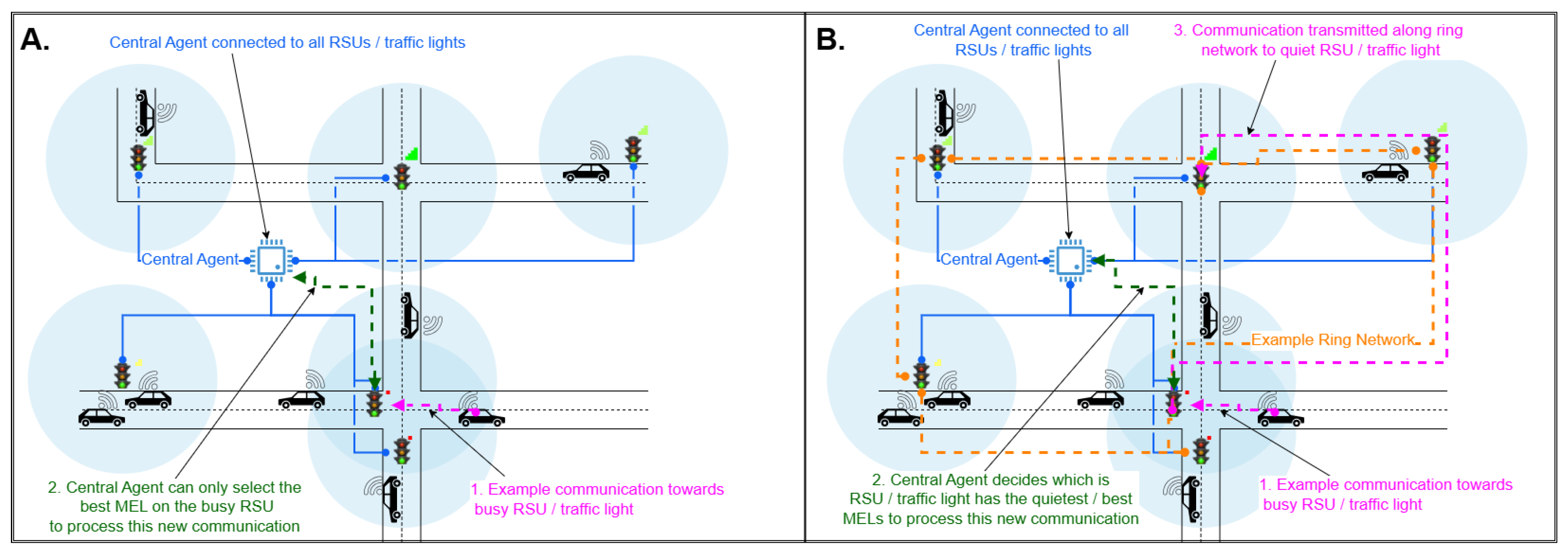
Figure 4.
Visualizing the start times, end times and number of active communications (ACs) for each of the 5 runs comparing the Nearest and Quietest architectures for both SPMB and MCFR.
Figure 4.
Visualizing the start times, end times and number of active communications (ACs) for each of the 5 runs comparing the Nearest and Quietest architectures for both SPMB and MCFR.
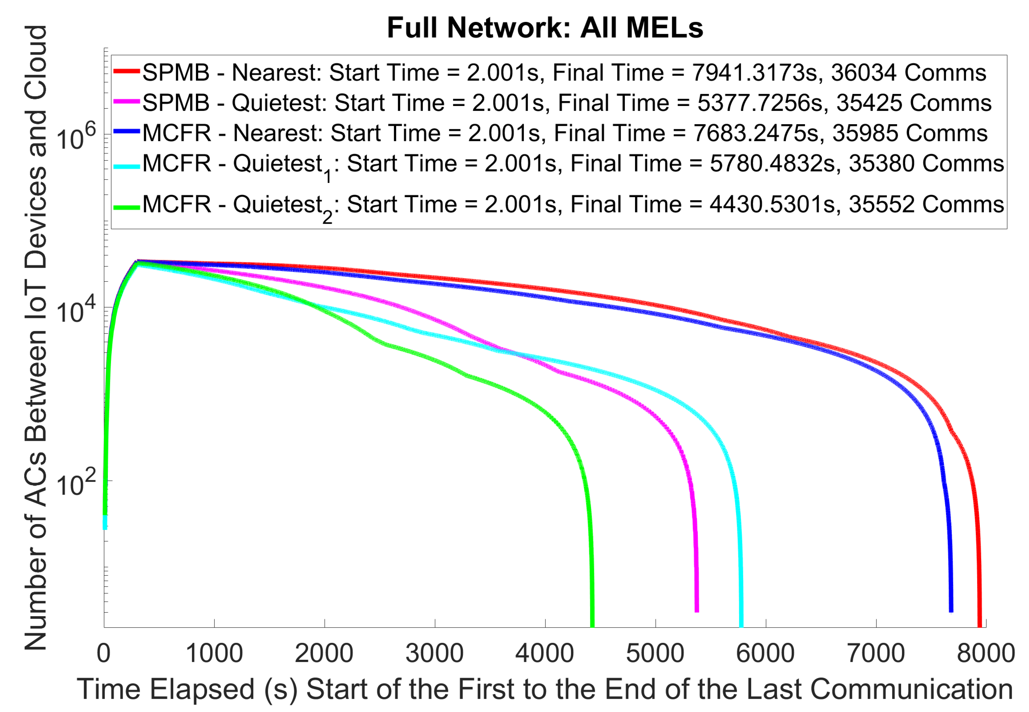
Figure 5.
Visualizing the impact of both the routing algorithm and network architecture on the edge processing times.
Figure 5.
Visualizing the impact of both the routing algorithm and network architecture on the edge processing times.

Figure 6.
The impact of routing algorithm over a specific architecture on the cloud processing times.
Figure 6.
The impact of routing algorithm over a specific architecture on the cloud processing times.
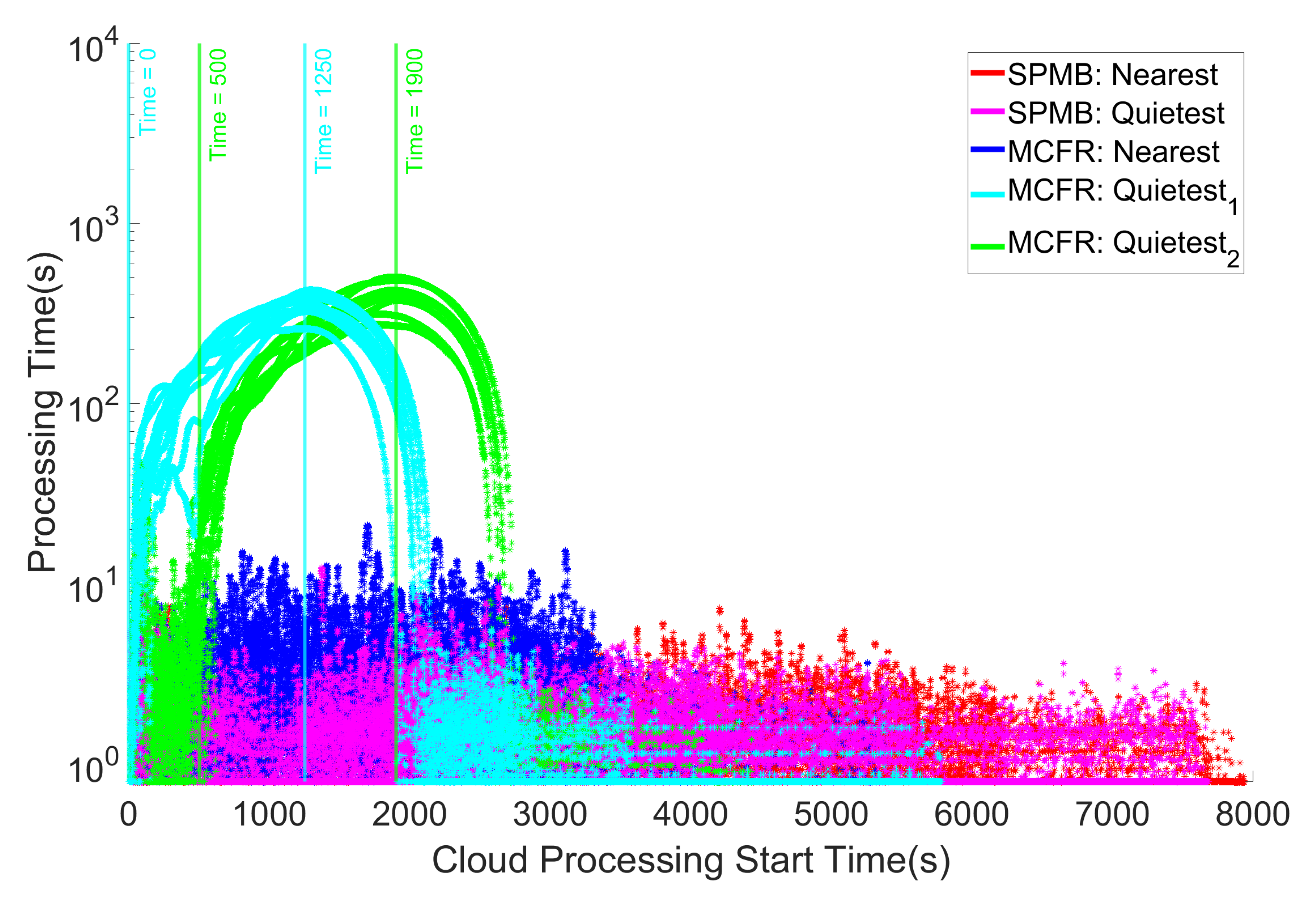
Figure 7.
Visualizing the start times, end times and number of active communications (ACs) between the MELs and the Cloud for each of the 5 runs comparing the Nearest and Quietest architectures for both SPMB and MCFR.
Figure 7.
Visualizing the start times, end times and number of active communications (ACs) between the MELs and the Cloud for each of the 5 runs comparing the Nearest and Quietest architectures for both SPMB and MCFR.
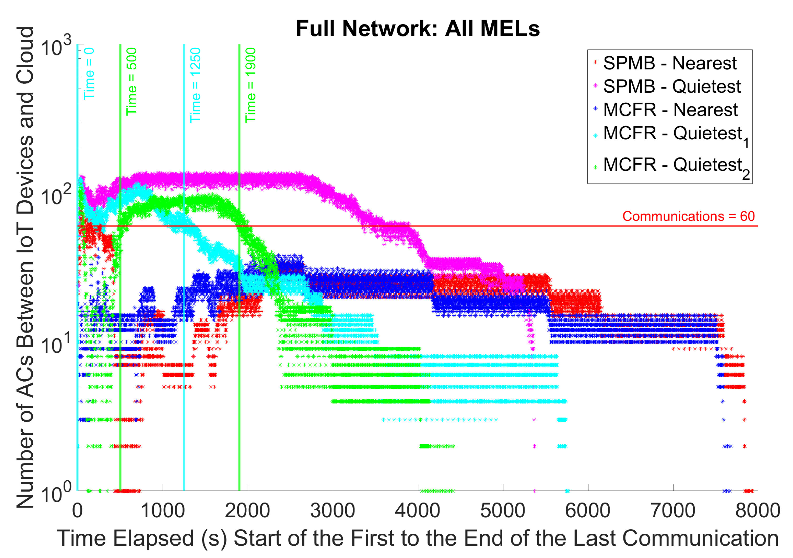

Table 1.
Packet Rate from IoT to the Cloud.
| Configuration | Communications per second |
|---|---|
| SPMB - Nearest | 4.54 |
| SPMB - Quietest | 6.59 |
| MCFR - Nearest | 4.68 |
| MCFR - Quietest | 6.12 |
| MCFR - Quietest | 8.02 |
Disclaimer/Publisher’s Note: The statements, opinions and data contained in all publications are solely those of the individual author(s) and contributor(s) and not of MDPI and/or the editor(s). MDPI and/or the editor(s) disclaim responsibility for any injury to people or property resulting from any ideas, methods, instructions or products referred to in the content. |
© 2025 by the authors. Licensee MDPI, Basel, Switzerland. This article is an open access article distributed under the terms and conditions of the Creative Commons Attribution (CC BY) license (http://creativecommons.org/licenses/by/4.0/).
Copyright: This open access article is published under a Creative Commons CC BY 4.0 license, which permit the free download, distribution, and reuse, provided that the author and preprint are cited in any reuse.


