
Submitted:
06 February 2025
Posted:
07 February 2025
You are already at the latest version
Abstract
A large group of people, nowadays, has been suffering from chronic sleep disorders and diseases, resulting in wide attention on sleep quality assessment. Conventional sleep-staging networks frequently consider multiple channel inputs, hindering the feasibility of the network to single-channel input or other sensor data input. In this paper, we proposed an Auto-SleepNet: a CPU-driven and end-to-end deep learning network for sleep stage classification using single-lead electroencephalogram (EEG) signals. The network is composed of a tailored Auto-Encoder for feature extraction and correction, and an LSTM network for temporal-signal classification. Compared with multi-lead connections, our design renders a higher accuracy in comparison to state-of-the-art, provides a meaningful reference for simplifying the hardware requirements of the EEG measurement device, and simultaneously lowers the computational loads significantly. We used the Per-Class precision (PR), Recall (RE), Per-Class F1 Score, overall accuracy, confusion matrix, and Cohen’s kappa coefficient (κ) to evaluate the performance. The overall accuracy, RE, and Cohen’s Kappa of our model are 95.7%, 95.19% and 0.91, respectively. Compared to state-of-the-art methods mentioned in the paper, Auto-SleepNet outperforms single-channel methods by 13.97%, and multiple-channel methods by 15.97% on average. Furthermore, it is not compulsory to use a GPU to train our Auto-SleepNet. Experiments show that our model can converge in 15.6 minutes using a CPU only. The results highlight the practicability of the network to sleep stage classification problems.
Keywords:
Deep Learning
; electroencephalogram
; Long Short-Term Memory
; Single-channel EEG
; Sleep Staging
1. Introduction
Sleep takes up around one-third of people’s lives, and good sleep quality can maintain one’s productive work throughout the day. Unfortunately, sleep deprivation and disorders are prevalent and strongly affect a substantial portion of the global population and impose significant welfare costs [1,2,3,4,5]. In the past decades, sleep staging mainly depended on the experience of human experts and symptoms reported by patients, which is, however, costly both for the government and the public, and prone to errors if the patients failed to describe their symptoms completely and accurately.
The classification of sleep stages aids in the understanding of brain states and unconscious processes [6]. There are mainly two sleep staging criteria that receive worldwide recognition. In 1968, Rechtschaffen and Kales (R&K) proposed a sleep staging method that divides sleep stages into Wake, rapid eye movement (REM), and non-REM (NREM) [7]. This criterion was later revised in 2007 by the American Academy of Sleep Medicine (AASM), which further divides NREM into three stages, namely N1, N2, N3 or S1, S2, and S3 [8].
In recent decades, deep learning has made great breakthroughs and an increasing number of conventional methods have begun to be surpassed by deep learning. The most seen method to identify sleep stages are multiple-channel approaches [20,21,22,29,33,35]. Using multiple-channel signals as input enjoys a higher accuracy in classification, because the network may have richer and more direct prior information. However, those methods increase the demand for the sleep dataset, which means patients should wear electrodes for several nights to collect at least a dozen channels of data, and the data should be annotated one-by-one by human experts. This requirement, unfortunately, is always not easy for scholars and organizations without collaborations with medical institutes, hindering the possibility of generalizing the method. As a result, the difficulty in acquiring sleep datasets has daunted scholars who even enjoy rich knowledge in the research field and therefore has become the most time-consuming part of sleep staging research. There is a potential meaning in single-channel sleep staging both in research and industrial fields, as the requirement for collecting the sleep dataset is much lower and the algorithm is easy to be implemented on portable devices for sleep quality assessment. Unfortunately, the network may not be able to obtain sufficient prior information from only one channel, which may bring the algorithm a lower classification accuracy than multi-channel methods [12,13,18,26,27,29,31,44].
We proposed a single-channel deep learning network that renders remarkably higher accuracy yet with lower computational loads, called Auto-SleepNet. The main contributions are as follows:
Auto-SleepNet is composed of a tailored Auto-Encoder and a Bi-directional Long Short-Term Memory (Bi-LSTM) network. The Auto-Encoder solves the overfitting problem presenting ubiquitously in the encoder-decoder structures by employing a novel design. Compared with the state-of-the-art, ours provides a higher accuracy in classifying sleep stages in comparison to state-of-the-art.
Training our Auto-SleepNet is easy. The model converges in a remarkably short time even using a CPU. Compared with state-of-the-art methods, our model does not necessarily require a GPU for training but can still outperform the state-of-the-art methods mentioned in this paper both in the results and convergence time.
We have also compared our method with multiple-channel ones. Contrary to the usual intuition, ours achieves a final classification accuracy of 95.7%, which has outperformed the state-of-the-art multiple-channel models significantly while leveraging less input information than those.
Since the property of our Auto-SleepNet is based on single-channel EEG for sleep staging of the subject, the complexity of manually analyzing multi-channel EEG signal is greatly reduced, reducing the cost of human resources and the possible cost of the EEG measurement device.
2. Methodology
2.1. Structure Overview
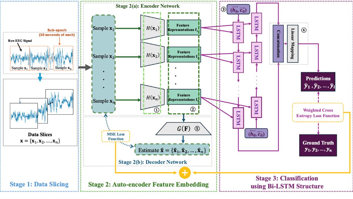
A detailed structure of Auto-SleepNet is shown in Figure 1. It consists of three main processes: data slicing, Auto-Encoder feature embedding, and classification using a Bi-LSTM network. The whole training process is driven by a combined loss function, i.e., a mean square error (MSE) loss function and a cross-entropy loss function. This deep neural network can be trained end-to-end for sleep stage classification. Different from other two-stage models [37,38,39], the proposed one tailors a stable training process, thus balancing the two training phases, namely the signal encoding phase and classification phase, and in turn avoiding the overfitting problem widely existing in the field of representation learning [40,41]. For the data slicing stage, each single-channel EEG signal is sliced into sub-epochs of 30 seconds each in an overlapped manner as recommended by AASM. Next, each sub-epoch is taken as input to the feature extraction network. This network is designed for dimensionality reduction while reserving the effective features as well as possible by comparing the restored signal with its corresponding original single-channel EEG input. In Stage 3, the extracted features are fed into an LSTM network. The features are regarded as a large vocabulary set, where each single-lead input is encoded as a short but lossless vector and the size of the whole training dataset is a vocabulary set. Therefore, this design can fully use the spatial and temporal correlation of each vector.
Figure 1b shows the way of resizing each original 1×3000 sub-epoch. We designed two Max-Pooling layers and one Dropout layer in the encoding phase, and symmetrically, restore the sub-epoch in the decoding phase by two Max-Unpooling layers with similar settings. The Dropout layer is embedded in Encoding Block 2. Experiments show that the final compression results can benefit from this structure, since redundant information in time domain can be reduced and compressed effectively, increasing the learning complexity and simultaneously preventing the network from learning the information irrelevant to the learning objective.
① Encoder network for the sliced data samples . It is noteworthy that the parameters of all the encoder networks are shared. The input and output details of the network can be seen in Figure 1b, and the network structure of the encoder and decoder can be seen in Figure 2a,b.
② The feature representations of each sliced data sample form a feature sequence , where are arranged in chronological order.
③ Initial state of the LSTM network, where is the initial hidden state and the initial cell of the forward pass. The initial state of the backward pass is represented by ().
④ Outputs of the two directions are concatenated and passed through fully connected layers to make predictions.
⑤ Decoder network for decoding the feature representations . The objective is to construct an unbiased and highly condensed representation of the sliced data samples by calculating the MSE between true data samples and the output from the decoder network.
Figure 1 The processing pipeline of the proposed method. The raw EEG signal is first sliced to several sub-epochs of 30 seconds each in an overlapped manner. The sliced epochs are taken as different training samples and fed into the Auto-Encoder feature embedder. The Auto-Encoder can encode the time-series data, i.e., 30-second sub-epochs, into efficient and highly condensed feature representations, which are then corrected by a decoder network and supervised by their own original input sub-epoch. The error between the Auto-Encoder output and the original input is calculated by an MSE loss function. In one training batch, all the feature representations are arranged in chronological order and fed into a Bi-directional LSTM network. Next, the two-directional outputs of the LSTM network are concatenated and linearly mapped to one-hot predictions of the classes. Finally, the true label is compared with the predicted label by calculating a cross-entropy loss function and the error is added with the MSE loss to form an end-to-end training.
2.2. Feature Encoding and Classification
A fundamental problem of sequence modeling is to compress context into a smaller vector [14]. The effectiveness of the encoding network directly affects the convergence speed of the entire model. As proved by our experiments and mentioned in the work [40,41], a naïve Auto-Encoder network is extremely easy to overfit, as it is oversimple for the model to learn some shortcuts irrelevant to the main training task, causing it to converge quickly in a different way than expected. The frequent practice is to create some barriers to the training, such as introducing noise to the input data, but the effects of those actions are extremely limited. Different from the above, we tailored a novel Auto-Encoder for data embedding which can effectively avoid overfitting by introducing several max-pooling and un-pooling layers and one dropout layer in the network, and by involving an end-to-end training strategy to balance the encoding and classification process so that the training cannot be stopped earlier than expected. Therefore, the proposed network is end-to-end trained and supervised by two combined loss functions. The data slicing is the initial step for classifying such time-series data. The encoder network is composed of two encoding blocks, two max pooling layers, and one hidden encoding block.
The method to process original EEG data is shown in Figure 2a. A single-channel EEG signal is sliced into 30-second sub-epochs in an overlapped manner. Then, each sub-epoch is treated as a data sample and fed into the Auto-Encoder. All the trainable parameters updated by those samples are sharable, hence the Auto-Encoders shown in Figure 2a can be seen as a model of a whole.
The encoder network is shown in Figure 2b. Borrowed an idea from the standard ResNet structure, in the first encoding block the kernel size of the convolutional layer is designed to be 50 and the stride is 6, because EEG signals are redundant in the time domain hence should be compressed as much as possible in the first stage to facilitate the learning efficiency. The two max pooling layers here can create barriers to the learning process and in turn avoid overfitting. In the final stage of the encoder network, the high-level features are passed through a hidden layer with the settings shown in the blue block in Figure 2b to obtain the feature representation .
Given a sequence of EEG epochs represented by , the sleep staging network is to model the conditional probability , where is the total number of sub-epochs in the dataset, each scalar in is the true sleep stage, and each vector in represents a 30-second EEG sub-epoch.
First, we apply data standardization to ensure that the training and testing datasets are from the same distribution. We standardize the original training data to remove the mean and scale it to unit variance, as depicted in Eq. (1):
where and are respectively the mean value and standard deviation of the training dataset. is the normalized dataset, and is the set of corresponding original sub-epochs. Note that the test dataset should also be normalized by the same training configuration because the mean and variance of the test dataset are not available prior to training.
Given a sequence of EEG epochs represented by , the sleep staging network is to model the conditional probability , where is the total number of sub-epochs in the dataset, each scalar in is the true sleep stage, and each vector in represents a 30-second EEG sub-epoch. We introduced an MSE loss function to achieve self-correction of the encoded sub-epochs, ensuring that the encoded features accurately represent the original data. The loss function for data encoding is shown in Eq. (2):
where represents the sub-epoch. stands for the estimate of the corresponding sub-epoch after going through the Auto-Encoder. represents the encoder network, while the decoder network. The objective of this Auto-Encoder is to learn a highly condensed and precise representation of the input sub-epoch, i.e., in Eq. (3):
As shown in Eq. (4), is the targeted chronological sequence of feature representation that will be fed into the classification network for sleep staging:
In the Auto-Encoder network, is the extracted representative feature matrix of the i-th 30-second PSG sub-epoch in the training dataset, and is arranged in chronological order, composing a feature sequence F.
Inspired by [45], in our network we also adopted a Bi-LSTM structure to ensure the temporal features can be fully extracted. The feature sequence F with hidden state is processed in both the forward and backward directions. Mathematically, the inputs and outputs of the LSTM network are given by Eq. (5):
where is the hidden state at time step , the cell of time , and the feature vector at time step in the feature sequence F, arranged in the same order as in . Before training the LSTM network, the hidden state and cell should be initialized to all zeros. To predict , the last hidden states are concatenated and fed into the fully connected layer to output the final predicted class.
2.3. Loss Functions for the End-to-End Training
Borrowing ideas from other remarkable work [47-50], we used a weighted cross entropy loss function to avoid the imbalance of the prediction. Eq. (6) explains the mechanism we used for balancing the weights of each class.
where represents the total number of samples in the training dataset, i.e., total number of sub-epochs, the true class of the current sub-epoch i, and the predicted class of the sub-epoch of the network. is the current true class, and is the total number of samples of class . The policy to give a weight to each class is , meaning that the weight to each class is inversely proportional to the number of samples of this class. Therefore, penalizes the classes with a clear numerical advantage over others by multiplying with the term .
End-to-end network training is desirable in this problem since it learns the global solution directly in contrast to multiple-stage training that estimates local solutions in separate stages. Our experiments have also proved that training in an end-to-end manner can avoid the overfitting problem of the Auto-Encoder more effectively than other typical operations, such as adding noise. The overall loss function for the training is given in Eq. (7).
where and are respectively the training coefficients that adjust the weights of the two loss functions in the training. In the real training process, we set and .
3. Evaluation
3.1. Dataset Organization
The public dataset we used for evaluation is the SleepEDFx dataset. The SleepEDFx dataset used in this study is a publicly available dataset that has been anonymized and made publicly available for research purposes. This is a collection of sleep recordings from healthy subjects contributed to PhysioNet and presented in European Data Format (EDF) [42]. It contains two types of PSG record, namely SC for 20 healthy subjects without sleep-related disorders and ST for 22 subjects of a study on Temazepam effects on sleep. Each record includes two-channel EEGs from the Fpz-Cz and Pz-Oz channels, a single-channel EOG, and a single-channel EMG. Each half-minute epoch is labeled as one of eight classes (W, REM, N1, N2, N3, N4, MOVEMENT, UNKNOWN) according to R&K rules [20,45].
A detailed enumeration of samples corresponding to the five sleep stages in SleepEDF is presented in Table 1.
After reorganizing the raw dataset into sub-epochs in 30 seconds, the sample size of each class is presented in Table 2.
3.2 Results Evaluation
The Auto-SleepNet was evaluated by the Per-Class precision (PR), Recall (RE), Per-Class F1 Score, overall accuracy (Acc. in Table 5), confusion matrix, and Cohen’s kappa coefficient (κ). The way to calculate those evaluation indices is given as follows:
where is the element in the i-th row and j-th column of the confusion matrix and c is the number of sleep stages, i.e., five stages in this study [9].
PR represents the prediction precision with which the model discriminates the current sleep stage from the others. RE represents the accuracy with which the model predicts the sleep stage. Overall accuracy represents the class-wise prediction accuracy of each class. Since F1 is calculated from the harmonic mean of the PE and RE, it can be more informative than the overall accuracy, especially in the case of an imbalanced class distribution. κ indicates the agreement between the true label and prediction, ranging between 0 and 1. The higher the value, the more consistent the true and prediction labels.
Table 3 shows the confusion matrix of our final training result. We summarized the result by performing 5-fold cross-validation. Confusion matrix is an effective method for evaluating classification performance by showing the accuracy rate of each class and cross-class. In Table 3, the expected result is that the larger the value on the diagonal, where ‘True Label’ and ‘Predicted Label’ overlap, the better the performance of this model. Auto-SleepNet shows a state-of-the-art performance in classifying the five sleep stages. For the class N1, the accuracy is slightly lower than others by virtue of the lack of training samples in the public dataset.
The averaged overall accuracy and RE are 95.7% and 95.19%, respectively. The rest of the results can be seen in Table 4, which compares our result with other state-of-the-art that use SleepEDF as the dataset. Auto-SleepNet has outperformed single-channel methods by 13.97%, and multiple-channel methods by 15.97% on average, in terms of the overall accuracy. Unlike the problem with other methods, where it is difficult to balance the training and test results, our method can show relatively better compatibility between the two. This is because the design of the Auto-Encoder can better explain the features of the data and the end-to-end mechanism fits the data more properly and efficiently. Furthermore, our model exhibits a relatively better convergence speed compared to other deep learning models.
Figure 3 displays the real-time sleep scoring of Auto-SleepNet. The blue line represents the classification result by Auto-SleepNet, while the orange line represents the true sleep stages. It can be seen that most of the sleep stages can be classified accurately.
We used a MacBook Pro equipped with 64-GiB memory and a graphics processing unit (GPU) for the training, yet our model can converge in a short time even without using a GPU, namely spending 15.6 minutes for convergence. Table 5 describes the machine specifications used to train Auto-SleepNet and state-of-the-art and the time spent by our model and others. Other models, however, mostly spent infinite time to converge using a central processing unit (CPU), therefore the specific time is replaced by a short dash ‘-’.
4. Conclusions
Sleep-related disorders have long plagued a large group of people of various ages, and sleep staging is of great significance for understanding human sleep status and improving sleep quality. In this study, we proposed an end-to-end automatic sleep staging network, called Auto-SleepNet, for single-lead sleep staging. Compared to other existed networks, ours achieves a significant improvement on sleep stage classification accuracy while simplifies the hardware requirement and lower the computational loads. This network would provide a meaningful reference for single-channel sleep staging problems. In the future, the application of Auto-SleepNet would make sleep staging more accessible to the public and researchers without professional equipment for collecting multiple-channel EEG signals.
Acknowledgments
The authors gratefully acknowledge the financial support of the non-wearable and non-invasive photonic sleep monitoring system based on an optical fiber sensor with machine learning (HKPU 1-WZ01) and the Shenzhen-Hong Kong-Macao Science and Technology Plan C SGDX (2020110309520303 K-ZGCQ).
References
- Perslev, M.; Darkner, S.; Kempfner, L.; Nikolic, M.; Jennum, P.J.; Igel, C. U-Sleep: resilient high-frequency sleep staging. npj Digit. Med. 2021, 4, 1–12. [Google Scholar] [CrossRef]
- Mousavi, S.; Afghah, F.; Acharya, U.R. SleepEEGNet: Automated sleep stage scoring with sequence to sequence deep learning approach. PLOS ONE 2019, 14, e0216456. [Google Scholar] [CrossRef] [PubMed]
- Ohayon, M.M. Epidemiology of insomnia: what we know and what we still need to learn. Sleep Med. Rev. 2002, 6, 97–111. [Google Scholar] [CrossRef] [PubMed]
- T. Roth, C. Coulouvrat, G. Hajak, et al., “Prevalence and perceived health associated with insomnia based on DSM-IV-TR; International Statistical Classification of Diseases and Related Health Problems, Tenth Revision; and Research Diagnostic Criteria/International Classification of Sleep Disorders, Second Edition criteria: results from the America Insomnia Survey”, Biological Psychiatry, 2011, 15; 69(6):592-600. [CrossRef]
- Phan, H.; Andreotti, F.; Cooray, N.; Chen, O.Y.; De Vos, M. SeqSleepNet: End-to-End Hierarchical Recurrent Neural Network for Sequence-to-Sequence Automatic Sleep Staging. IEEE Trans. Neural Syst. Rehabil. Eng. 2019, 27, 400–410. [Google Scholar] [CrossRef] [PubMed]
- M. Jones, V. L. Itti, and B. R. Sheth, Electrocardiogram sleep staging on par with expert polysomnography. Cold Spring Harbor Laboratory Press, 2023, 2023. [CrossRef]
- Wolpert, E.A. A Manual of Standardized Terminology, Techniques and Scoring System for Sleep Stages of Human Subjects. Arch. Gen. Psychiatry 1969, 20, 246–247. [Google Scholar] [CrossRef]
- R. B. Berry, et al., “The AASM manual for the scoring of sleep and associated events”, Rules, Terminology and Technical Specifications, Darien, Illinois, American Academy of Sleep Medicine, 2012, 176.2012(2012): 7.
- M, H.; M.N, S. A Review on Evaluation Metrics for Data Classification Evaluations. Int. J. Data Min. Knowl. Manag. Process. 2015, 5, 01–11. [CrossRef]
- S., C.V.; E., R. A Novel Deep Learning based Gated Recurrent Unit with Extreme Learning Machine for Electrocardiogram (ECG) Signal Recognition. Biomed. Signal Process. Control. 2021, 68. [CrossRef]
- Liu, Y.; Lin, Y.; Jia, Z.; Wang, J.; Ma, Y. A new dissimilarity measure based on ordinal pattern for analyzing physiological signals. Phys. A: Stat. Mech. its Appl. 2021, 574. [Google Scholar] [CrossRef]
- Supratak, A.; Dong, H.; Wu, C.; Guo, Y. DeepSleepNet: A Model for Automatic Sleep Stage Scoring Based on Raw Single-Channel EEG. IEEE Trans. Neural Syst. Rehabil. Eng. 2017, 25, 1998–2008. [Google Scholar] [CrossRef]
- Supratak and, Y. Guo, “TinySleepNet: An Efficient Deep Learning Model for Sleep Stage Scoring based on Raw Single-Channel EEG,” Annu. Int. Conf. IEEE Eng. Med. Biol. Soc., vol. 2020, pp. 641–644, Jul. 2020. [CrossRef]
- M. Perslev, M. H. Jensen, S. Darkner, et al., “Utime: A fully convolutional network for time series segmentation applied to sleep staging,” Adv. Neural Inf. Process. Syst., vol. 32, pp. 4415–4426, 2019.
- Phan, H.; Andreotti, F.; Cooray, N.; Chen, O.Y.; De Vos, M. DNN Filter Bank Improves 1-Max Pooling CNN for Single-Channel EEG Automatic Sleep Stage Classification. In Proceedings of the 2018 40th Annual International Conference of the IEEE Engineering in Medicine and Biology Society (EMBC), Honolulu, HI, USA, 18–21 July 2018; pp. 453–456. [Google Scholar]
- Andreotti, F.; Phan, H.; Cooray, N.; Lo, C.; Hu, M.T.M.; De Vos, M. Multichannel Sleep Stage Classification and Transfer Learning using Convolutional Neural Networks. In Proceedings of the 2018 40th Annual International Conference of the IEEE Engineering in Medicine and Biology Society (EMBC), Honolulu, HI, USA, 18–21 July 2018. [Google Scholar]
- Tsinalis, O.; Matthews, P.M.; Guo, Y. Automatic Sleep Stage Scoring Using Time-Frequency Analysis and Stacked Sparse Autoencoders. Ann. Biomed. Eng. 2015, 44, 1587–1597. [Google Scholar] [CrossRef]
- Lee, S.; Yu, Y.; Back, S.; Seo, H.; Lee, K. SleePyCo: Automatic sleep scoring with feature pyramid and contrastive learning. Expert Syst. Appl. 2023, 240. [Google Scholar] [CrossRef]
- Phan, H.; Chen, O.Y.; Tran, M.C.; Koch, P.; Mertins, A.; De Vos, M. XSleepNet: Multi-View Sequential Model for Automatic Sleep Staging. IEEE Trans. Pattern Anal. Mach. Intell. 2021, 44, 1–1. [Google Scholar] [CrossRef]
- S. A. Imtiaz and E. Rodriguez-Villegas, “An open-source toolbox for standardized use of PhysioNet Sleep EDF Expanded Database,” Annu. Int. Conf. IEEE Eng. Med. Biol. Soc., vol. 2015, pp. 6014–6017, 2015. [CrossRef]
- Phan, H., Mikkelsen K., Oliver Y. C., Philipp Koch, Alfred Mertins, and Maarten D. V., “SleepTransformer: Automatic Sleep Staging with Interpretability and Uncertainty Quantification”, 2021.
- Li, Y.; Xu, Z.; Zhang, Y.; Cao, Z.; Chen, H. Automatic sleep stage classification based on a two-channel electrooculogram and one-channel electromyogram. Physiol. Meas. 2022, 43, 07NT02. [Google Scholar] [CrossRef] [PubMed]
- Satapathy, S.K.; Loganathan, D. Multimodal Multiclass Machine Learning Model for Automated Sleep Staging Based on Time Series Data. SN Comput. Sci. 2022, 3, 1–20. [Google Scholar] [CrossRef]
- Yang, C.; Xiao, C.; Westover, M.B.; Sun, J. Self-Supervised Electroencephalogram Representation Learning for Automatic Sleep Staging: Model Development and Evaluation Study. JMIR AI 2023, 2, e46769. [Google Scholar] [CrossRef] [PubMed]
- An, P.; Yuan, Z.; Zhao, J.; Jiang, X.; Du, B. An effective multi-model fusion method for EEG-based sleep stage classification. Knowledge-Based Syst. 2021, 219, 106890. [Google Scholar] [CrossRef]
- Tang, M.; Zhang, Z.; He, Z.; Li, W.; Mou, X.; Du, L.; Wang, P.; Zhao, Z.; Chen, X.; Li, X.; et al. Deep adaptation network for subject-specific sleep stage classification based on a single-lead ECG. Biomed. Signal Process. Control. 2022, 75, 106890. [Google Scholar] [CrossRef]
- Urtnasan, E.; Park, J.-U.; Joo, E.Y.; Lee, K.-J. Deep Convolutional Recurrent Model for Automatic Scoring Sleep Stages Based on Single-Lead ECG Signal. Diagnostics 2022, 12, 1235. [Google Scholar] [CrossRef]
- X. Cai, Z. Jia, and Z. Jiao, “Two-Stream Squeeze-and-Excitation Network for Multi-modal Sleep Staging”, 2021 IEEE International Conference on Bioinformatics and Biomedicine (BIBM), 2021, 1262-1265. [CrossRef]
- Fan, J.; Sun, C.; Long, M.; Chen, C.; Chen, W. EOGNET: A Novel Deep Learning Model for Sleep Stage Classification Based on Single-Channel EOG Signal. Front. Neurosci. 2021, 15, 573194. [Google Scholar] [CrossRef]
- M. Dutt, M. Goodwin, and C. Omlin, “Automatic Sleep Stage Identification with Time Distributed Convolutional Neural Network”, 2021 International Joint Conference on Neural Networks (IJCNN), 2021, 1-7. [CrossRef]
- Kuo, C.-E.; Chen, G.-T.; Liao, P.-Y. An EEG spectrogram-based automatic sleep stage scoring method via data augmentation, ensemble convolution neural network, and expert knowledge. Biomed. Signal Process. Control. 2021, 70, 102981. [Google Scholar] [CrossRef]
- Sun, C.; Fan, J.; Chen, C.; Li, W.; Chen, W. A Two-Stage Neural Network for Sleep Stage Classification Based on Feature Learning, Sequence Learning, and Data Augmentation. IEEE Access 2019, 7, 109386–109397. [Google Scholar] [CrossRef]
- Abdollahpour, M.; Rezaii, T.Y.; Farzamnia, A.; Saad, I. Transfer Learning Convolutional Neural Network for Sleep Stage Classification Using Two-Stage Data Fusion Framework. IEEE Access 2020, 8, 180618–180632. [Google Scholar] [CrossRef]
- H. Xi, Y. Wang, S. Cui, and R. Niu, “Two-stage Multi-task Learning for Automatic Sleep Staging Method”, Proceedings of the 2021 4th International Conference on Artificial Intelligence and Pattern Recognition, 2021, 710-715. [CrossRef]
- Bengio, Y.; Courville, A.; Vincent, P. Representation Learning: A Review and New Perspectives. IEEE Trans. Pattern Anal. Mach. Intell. 2013, 35, 1798–1828. [Google Scholar] [CrossRef]
- Mandal, M.; Vipparthi, S.K. An Empirical Review of Deep Learning Frameworks for Change Detection: Model Design, Experimental Frameworks, Challenges and Research Needs. IEEE Trans. Intell. Transp. Syst. 2021, 23, 6101–6122. [Google Scholar] [CrossRef]
- Malan, N.; Sharma, S. Motor Imagery EEG Spectral-Spatial Feature Optimization Using Dual-Tree Complex Wavelet and Neighbourhood Component Analysis. IRBM 2022, 43, 198–209. [Google Scholar] [CrossRef]
- Zhou, D.; Xu, Q.; Zhang, J.; Wu, L.; Xu, H.; Kettunen, L.; Chang, Z.; Zhang, Q.; Cong, F. Interpretable Sleep Stage Classification Based on Layer-Wise Relevance Propagation. IEEE Trans. Instrum. Meas. 2024, 73, 1–10. [Google Scholar] [CrossRef]
- Zhou, D.; Xu, Q.; Wang, J.; Xu, H.; Kettunen, L.; Chang, Z.; Cong, F. Alleviating Class Imbalance Problem in Automatic Sleep Stage Classification. IEEE Trans. Instrum. Meas. 2022, 71, 1–12. [Google Scholar] [CrossRef]
- Q. Xu, D. Zhou, J. Wang, J. Shen, L. Kettunen, and F. Cong, “Convolutional Neural Network Based Sleep Stage Classification with Class Imbalance”, 2022 International Joint Conference on Neural Networks (IJCNN), Padua, Italy, 2022: 1-6. [CrossRef]
- Zhou, D.; Wang, J.; Hu, G.; Zhang, J.; Li, F.; Yan, R.; Kettunen, L.; Chang, Z.; Xu, Q.; Cong, F. SingleChannelNet: A model for automatic sleep stage classification with raw single-channel EEG. Biomed. Signal Process. Control. 2022, 75, 103592. [Google Scholar] [CrossRef]
- Kemp, B.; Zwinderman, A.; Tuk, B.; Kamphuisen, H.; Oberye, J. Analysis of a sleep-dependent neuronal feedback loop: the slow-wave microcontinuity of the EEG. IEEE Trans. Biomed. Eng. 2000, 47, 1185–1194. [Google Scholar] [CrossRef]
- Korkalainen, H.; Leppanen, T.; Duce, B.; Kainulainen, S.; Aakko, J.; Leino, A.; Kalevo, L.; Afara, I.O.; Myllymaa, S.; Toyras, J. Detailed Assessment of Sleep Architecture With Deep Learning and Shorter Epoch-to-Epoch Duration Reveals Sleep Fragmentation of Patients With Obstructive Sleep Apnea. IEEE J. Biomed. Heal. Informatics 2020, 25, 2567–2574. [Google Scholar] [CrossRef]
- T. Pham and R. Mouček, "Automatic Sleep Stage Classification by CNN-Transformer-LSTM using single-channel EEG signal," 2023 IEEE International Conference on Bioinformatics and Biomedicine (BIBM), Istanbul, Turkiye, 2023, pp. 2559-2563. [CrossRef]
- Seo, H.; Back, S.; Lee, S.; Park, D.; Kim, T.; Lee, K. Intra- and inter-epoch temporal context network (IITNet) using sub-epoch features for automatic sleep scoring on raw single-channel EEG. Biomed. Signal Process. Control. 2020, 61, 102037. [Google Scholar] [CrossRef]
Figure 1.
(a) Overview of the proposed network. (b) The input and output of the Auto-Encoder (left), and a zoomed-in comparison between the two (right).
Figure 1.
(a) Overview of the proposed network. (b) The input and output of the Auto-Encoder (left), and a zoomed-in comparison between the two (right).
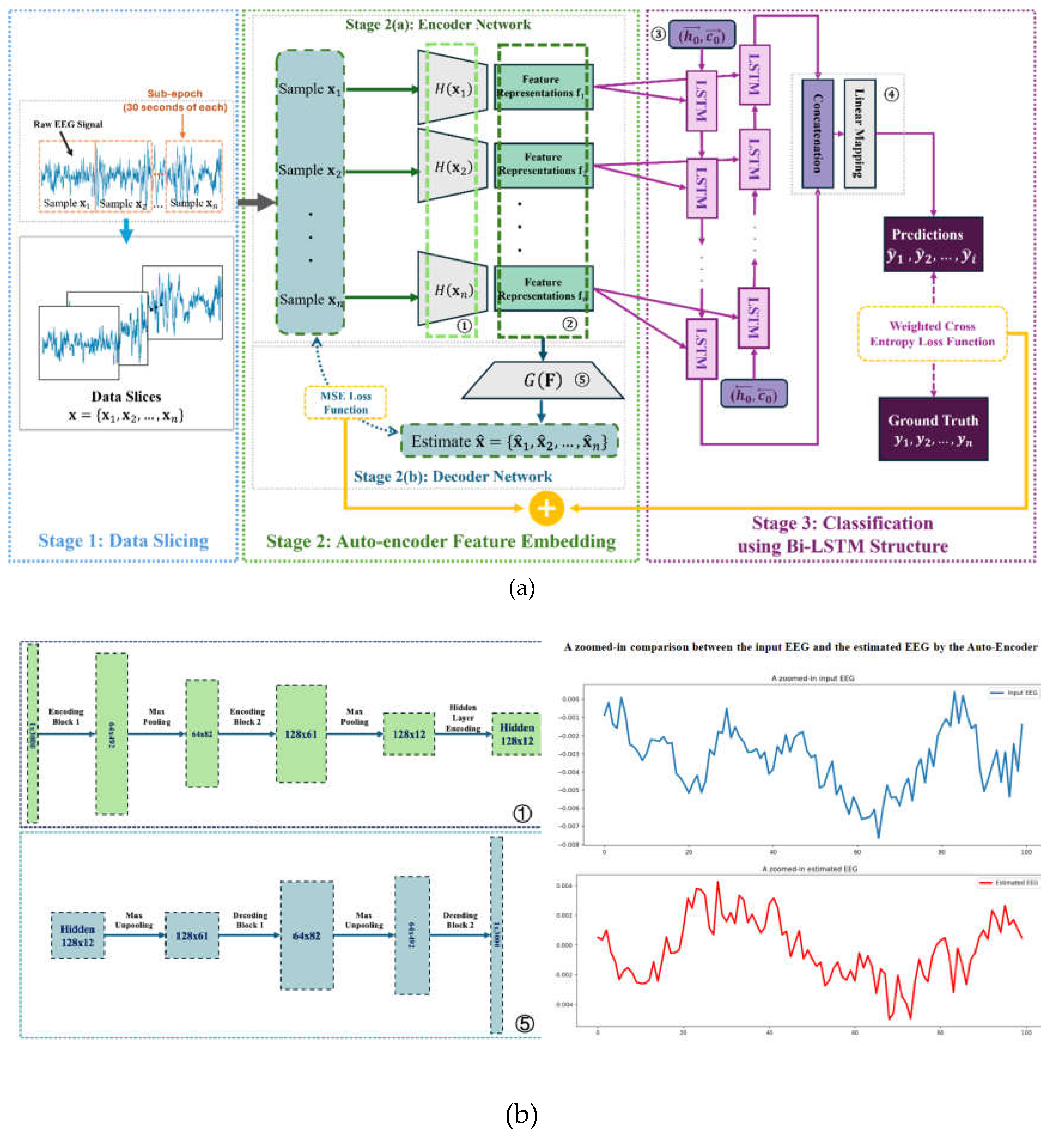
Figure 2.
(a) Data slicing method. (b) Detailed structure of the encoder network. In practice, the learnable parameters are sharable among each encoder. (c) Detailed structure of the decoder network. In practice, the learnable parameters are sharable among each decoder.
Figure 2.
(a) Data slicing method. (b) Detailed structure of the encoder network. In practice, the learnable parameters are sharable among each encoder. (c) Detailed structure of the decoder network. In practice, the learnable parameters are sharable among each decoder.
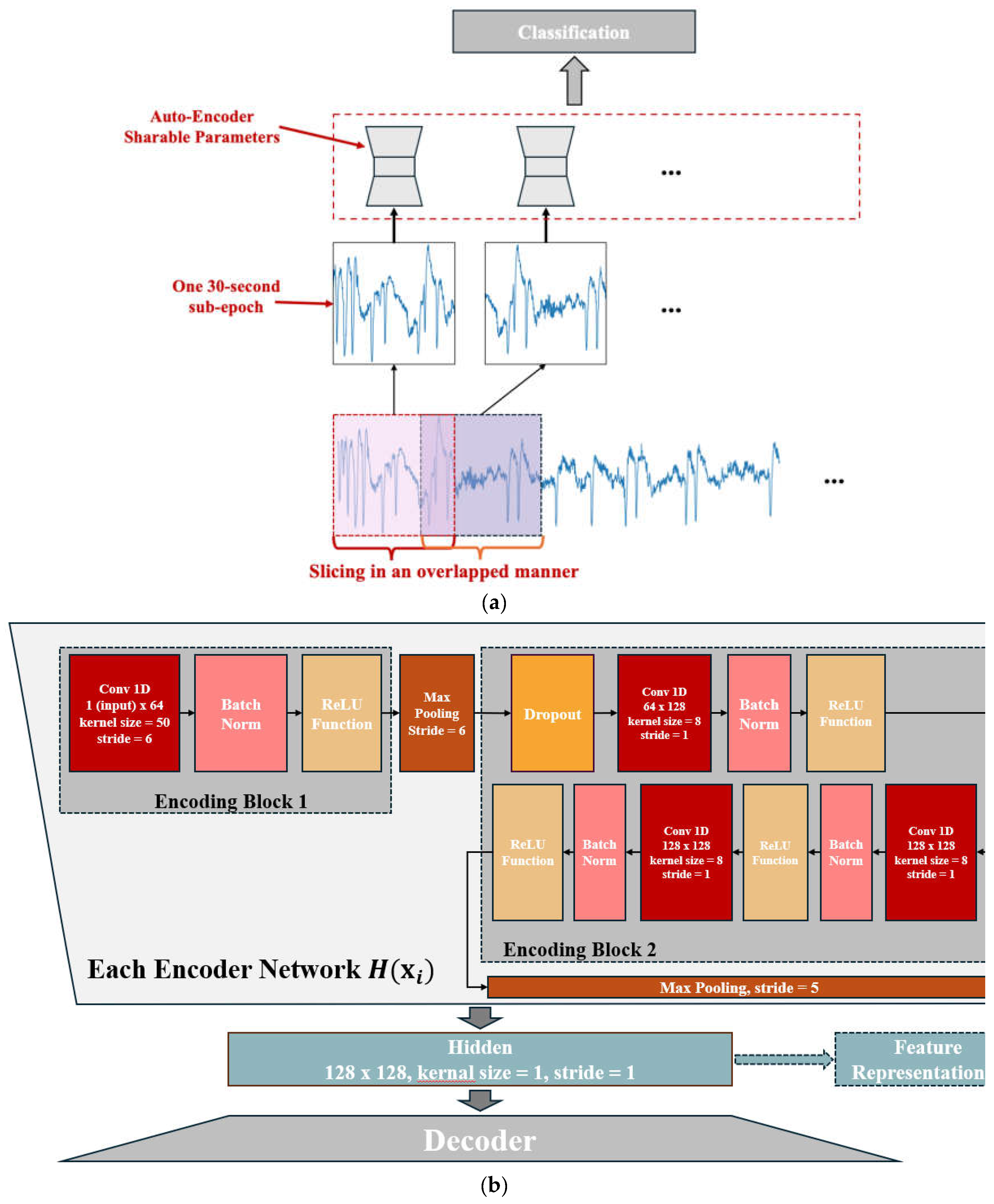
Figure 3.
Real-time sleep scoring of Auto-SleepNet.
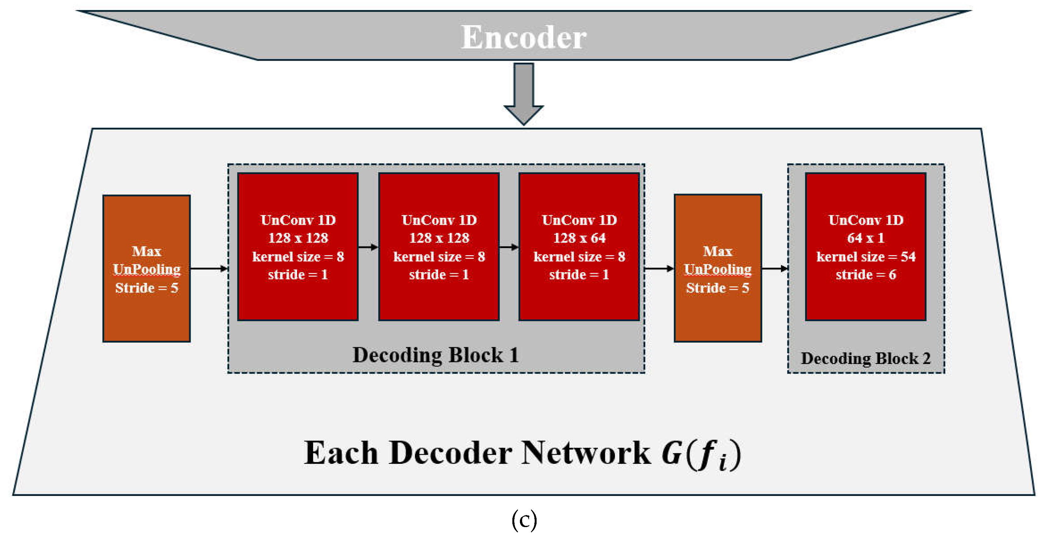

Table 1.
Sample size of each sleep class (the length of each data sample is ).
| Dataset | W | N1 | N2 | N3 | REM | Total |
|---|---|---|---|---|---|---|
| SleepEDF | 8,285 (20%) |
2,804 (7%) |
17,799 (42%) |
5,703 (13%) |
7,717 (18%) |
42,308 |
Table 2.
The class-wise number of 30-second sub-epochs after the reorganization.
| Class | W | N1 | N2 | N3 | REM |
|---|---|---|---|---|---|
| Number of Training Samples | 53,574 | 2,149 | 13,034 | 4,242 | 5,665 |
| Number of Test Samples | 14,178 | 571 | 3,485 | 1,062 | 1,460 |
Table 3.
Confusion matrix of the averaged training result.
| True Label | Predicted Label | ||||
|---|---|---|---|---|---|
| W | N1 | N2 | N3 | REM | |
| W | 14,009 | 28 | 48 | 16 | 77 |
| N1 | 75 | 267 | 77 | 0 | 152 |
| N2 | 24 | 22 | 3,151 | 98 | 190 |
| N3 | 4 | 0 | 136 | 922 | 0 |
| REM | 23 | 76 | 142 | 1 | 1,218 |
Table 4.
Comparisons between our model and other state-of-the-art.
| Method | EEG Dataset | Input Channel | Acc. (%) | Per-Class F1 Score (%) | Cohen’s Kappa | ||||
|---|---|---|---|---|---|---|---|---|---|
| W | N1 | N2 | N3 | REM | |||||
| Our Method | SleepEDF | Single | 95.7 | 99.0 | 35.0 | 89.0 | 89.0 | 78.0 | 0.91 |
| IITNet [45] | SleepEDF | Single | 83.6 | 84.7 | 29.8 | 86.3 | 87.1 | 72.8 | 0.77 |
| SleePyCo [18] | SleepEDF | Single | 84.6 | 93.5 | 50.4 | 86.5 | 80.5 | 84.2 | 0.79 |
| SleepTransformer [21] | SleepEDF | Single | 81.4 | 91.7 | 40.4 | 84.3 | 77.9 | 77.2 | 0.74 |
| TinySleepNet [13] | SleepEDF | Single | 83.1 | 92.8 | 51.0 | 85.3 | 81.1 | 80.3 | 0.77 |
| U-Time [14] | SleepEDF | Single | 81.3 | 92.0 | 51.0 | 83.5 | 74.6 | 80.2 | 0.75 |
| SleepEEGNet [46] | SleepEDF | Single | 80.0 | 91.7 | 44.1 | 82.5 | 73.5 | 76.1 | 0.73 |
| DeepSleepNet [12] | SleepEDF | Single | 82.0 | 84.7 | 46.6 | 85.9 | 84.8 | 82.4 | 0.76 |
| Phan et al [15] | SleepEDF | Multiple | 79.8 | - | - | - | - | - | - |
| Andreotti et al [16] | SleepEDF | Multiple | 76.8 | - | - | - | - | - | - |
| Tsinalis et al [17] | SleepEDF | Multiple | 78.9 | - | - | - | - | - | - |
| XSleepNet [19] | SleepEDF | Multiple | 84.0 | 93.3 | 49.9 | 86.0 | 78.7 | 81.8 | 0.78 |
| SeqSleepNet [5] | SleepEDF | Multiple | 82.6 | - | - | - | - | - | 0.76 |
Table 5.
Comparison with other models in terms of machine specifications.
| Method | Memory Usage for the Evaluation | GPU | Network Size | Time to Converge by GPU (Min.) | Time to Converge by CPU (Min.) |
|---|---|---|---|---|---|
| Ours | 64 GiB | Optional | 2.39 MB | 4.00 | 15.6 |
| IITNet [45] | 64 GiB | Compulsory | 40.4 MB | 111.09 | - |
| SleePyCo [23] | 64 GiB | Compulsory | 194 MB | 523.03 | - |
| SleepTransformer[26] | 64 GiB | Compulsory | 39.7 MB | 200.30 | - |
| TinySleepNet [13] | 64 GiB | Compulsory | 56.6 MB | 230.04 | - |
| U-Time [14] | 64 GiB | Compulsory | 300 MB | 220.03 | - |
| SleepEEGNet [46] | 64 GiB | Compulsory | 68.9 MB | 370.70 | - |
| DeepSleepNet [12] | 64 GiB | Compulsory | 59.9 MB | 270.00 | - |
| Phan et al [15] | 64 GiB | Compulsory | 49.00 MB | 110.10 | - |
| Andreotti et al [16] | 64 GiB | Compulsory | 89.9 MB | 260.10 | - |
| Tsinalis et al [17] | 64 GiB | Compulsory | 48.8 MB | 170.05 | - |
| XSleepNet [19] | 64 GiB | Compulsory | 66.8 MB | 260.60 | - |
| SeqSleepNet [5] | 64 GiB | Compulsory | 76.8 MB | 220.20 | - |
Disclaimer/Publisher’s Note: The statements, opinions and data contained in all publications are solely those of the individual author(s) and contributor(s) and not of MDPI and/or the editor(s). MDPI and/or the editor(s) disclaim responsibility for any injury to people or property resulting from any ideas, methods, instructions or products referred to in the content. |
© 2025 by the authors. Licensee MDPI, Basel, Switzerland. This article is an open access article distributed under the terms and conditions of the Creative Commons Attribution (CC BY) license (http://creativecommons.org/licenses/by/4.0/).
Copyright: This open access article is published under a Creative Commons CC BY 4.0 license, which permit the free download, distribution, and reuse, provided that the author and preprint are cited in any reuse.


