Submitted:
05 February 2025
Posted:
06 February 2025
You are already at the latest version
Abstract
Cancer is a major global health concern and one of the leading causes of death worldwide. As such, the study of cancer treatment and control has become an essential area of research in biomedical engineering. One critical aspect of cancer treatment is the prevention of cancer cell proliferation. This article proposes a novel approach in a cancer model with zero initial conditions once and another with random initial conditions by a Model Predictive Controller(MPC) developed by Reinforcement Learning. Models are treated by 3 different treatment methods including chemotherapy, anti-angiogenic and the combination of both treatment methods is used to evaluate the effectiveness and reduction of the number of cancer cells and the improvement of disease outcomes. Our results show that although chemotherapy is necessary to weaken cancer cells, the combination of both treatment methods reduces the number of cancer cells by approximately 65%, and this shows the effectiveness of the combination of two treatment methods with the help of a Model Predictive Controller(MPC) developed by Reinforcement Learning by reducing the number of tumor cells in the targeted location.
Keywords:
Chemotherapy
; Anti-angiogenic
; Model Predictive Control
; Reinforcement Learning
1. Introduction
Cancer is one of the most pressing health challenges of our time. It is the second leading cause of death worldwide, with millions of new cases diagnosed every year. Despite significant advances in cancer treatment and research, much remains to be done to find effective treatments [11]. Several types of cancer treatment methods exist, including surgery, immunotherapy, radiotherapy, chemotherapy, and others. Surgery is often the most effective treatment for localized tumors in the early stages [4], as it can remove the tumor completely. However, it cannot be used in cases of metastasis, and there is also a risk of damage to adjacent tissues.
Methods such as radiotherapy and chemotherapy are therapeutic methods based on targeted molecular therapy. Chemotherapy is the most common cancer treatment method [4,22] and, in some cases, the only treatment available. In chemotherapy and radiotherapy: 1. Cancer cells tend to grow rapidly, and chemotherapy drugs also work based on the mechanism of rapidly destroying growing cells, and since these drugs move throughout the body, they can also affect normal and healthy cells that are growing rapidly. Therefore, damage to healthy cells is the main side effect of chemotherapy and radiotherapy. 2. Cancer cells change shape to survive during chemotherapy treatment, so chemotherapy is often stopped alone [11].
In recent years, a new type of immunotherapy has emerged that targets the blood vessels that supply tumours with nutrients and oxygen. This therapy is known as anti-angiogenic therapy and has shown great promise in the fight against cancer. Anti-angiogenic therapy is a form of molecular targeted therapy that drugs prevent the formation of new blood vessels to feed the tumour and also prevent tumour growth to a critical level [1,7,12,19]. Compared to other treatments, one of the main advantages of anti-angiogenic therapy is that tumor cells do not become resistant to anti-angiogenic drugs. Also, anti-angiogenic drugs have less side effects on patients due to their non-toxicity. [11]. However, it is important to note that anti-angiogenic therapy does not remove the entire tumor but only stops its growth and keeps it at the initial stage. Therefore, this method is usually used in combination with conventional methods to remove the entire tumor [13,19]. Among other cancer treatment methods in the last few decades, we can mention immunotherapy, which has become an important part of treating some types of cancer. This treatment uses the body’s immune system to treat cancer with fewer side effects than targeted molecular treatments, such as chemotherapy [2,3]. However, despite the many available treatment methods and the disadvantages of each method, combination therapy as an optimal treatment method is still an open issue.
There are various mathematical models to investigate the interaction between tumor and immune system [4], for example, Kuznetsov et al. [5], de Vladar & González [6], Stepanova’s classic article and Hahnfeldt’s dynamic tumor growth model [14]. In an article published in 1999 [14], a simple system with a few ordinary differential equations was presented by Hahnfeldt et al., which described the growth of tumor cell numbers in the presence of an angiogenesis inhibitor as a treatment. With the help of this model and selection of inputs, the interaction between tumor growth and immune system activity during cancer development is described. This model was then modified in articles in 2005, 2011 and 2012 [15-17]. One of the key findings of this model is that for small volumes of cancer, the immune system can effectively control cancer growth. However, for larger cancer volumes, cancer dynamics can suppress immune dynamics. This highlights the importance of combining different treatment methods to achieve optimal results.
The use of controllers in cancer treatment is common. Among the controllers, the multiple model predictive controller (MMPC) was used in a 2017 article to determine the optimal treatment plan for a combination of chemotherapy and immunotherapy in the modified Stepanova model [10]. The results showed that the use of MMPC led to a decrease in tumor volume and drug dosage, making it an efficient strategy. In the article [9], which was published in 2020, unlike the rest of the articles that used the optimal control strategy, a positive T-S phase controller was proposed for the combined treatment of cancer under combined immunotherapy and chemotherapy, and It has been found that the volume of tumor cells and the doses of drugs used have been reduced to a minimum. These findings demonstrate the potential of using controllers in cancer treatment to optimize treatment plans and improve patient outcomes.
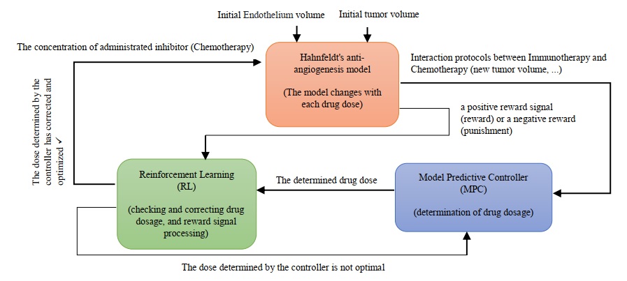
Cancer treatment has been challenging due to the complex and dynamic nature of the human body and the cancer system. The constantly changing environment and the activity of cancer cells make it difficult to develop effective treatments. Despite the numerous treatments and methods available, cancer has not been completely eliminated, and at best, its size has been fixed or reduced. This is due to uncertainties, disturbances, and unknown factors that have not been considered in the treatment process. To address this challenge, we used two treatment methods, chemotherapy and anti-angiogenesis, as a branch of immunotherapy, and then the combination of each method as cancer treatment methods. We propose a new approach that utilizes reinforcement learning (RL) to develop a predictive controller for determining the drug dosage amount that can be most effective at any moment. RL is a learning technique that enables an agent to learn through interaction with the environment and determine the best action to take in any situation to achieve optimal results. Therefore, the uncertainty factor is eliminated by this method. We have developed a model predictive controller with the concept of reinforcement learning to determine the dosage amount of the drug that can be most effective at any moment according to the unstable conditions of the system. Also, MPC is proposed to achieve this goal, which can be used for both immunotherapy and chemotherapy. The efficiency of the method is shown through simulation. As shown here, these results will help guide the development of combination therapies. In a general view, the research method is shown in Figure 1.
The rest of this paper is organized as follows: Section 2 provides a description of the model and the control problem. In Section 3, a controller is developed based on the model predictive control scheme with the concept of reinforcement learning. The simulation results and discussion are presented in section 4. Finally, conclusions are presented in Section 5.
2. Materials and Methods
In this part, the system model is explained and then we examine the problem of the controller.
2.1. Model of Tumor Dynamic Growth
We consider the dynamic model of tumor growth under anti-angiogenic therapy first developed in 1999 by Hahnfeldt et al. [14]. The developed nonlinear dynamic model is presented at [16]. By adding integrated administrated inhibitor as a new term to the model [17] and assuming that the clearance rate of the administrated inhibitor is known, the final and simpler dynamic model of tumor growth under angiogenesis inhibitor can be described as follows [12,15,18]:
(1)
The endothelium is a single layer of squamous endothelial cells that line the interior surface of blood vessels and lymphatic vessels. The model parameters values are presented in Table 1.
2.2. Controller İmplementation Problem
The main goal of anti-cancer drugs is to reduce tumor cells, but at the same time, it has destructive effects on the body Therefore, it is necessary to design an MPC controller based on RL to combine treatment methods, so that RL can modify the drug dose to have the most optimal effect on MPC performance. However, we will achieve the best dose of drug injection for less damage to the body and also to speed up the healing process.
2.3. Controller Design
In this section, the goal is to implement a controller in such a way that it can correct its performance in the most optimal way according to the existing conditions at any moment.
The most important benefit of this controller compared to the rest of them is that it can deal with the limitations directly and effectively. [20]. The way the MPC works is that it can predict the next output of the control system using the inputs and outputs from the previous process and thus provide a real-time solution to the problem. The MPC base algorithm is shown in Figure 2, as described in [21].
2.4. Model Predictive Controller
As mentioned, MPC predicts the output according to the input and previous output of the process and its goal is to minimize the difference between the predicted path and the desired path. MPC performs this action with a series of calculations and execution on control actions and placing the predicted path under the constraints. An important step to design MPC is to set an objective function, which is defined as follows:
(2)
The limitations of this system are as follows:
By definition of the chemotherapy and anti-angiogenic agents, the following inequalities are obtained if the maximum dose rates become normalize to 1:
(3)
(4)
The tumour volume and the immune-competent cell density can be positive or zero.
(5)
(6)
3. Theory and Calculation
3.1. Reinforcement Learning-Based Model Predictive Controller Design
Designing an optimal model-based controller for nonlinear systems is one of the most challenging problems in the control theory. In this section, a Reinforcement Learning-based Model Predictive controller is developed for cancer therapy.
Reinforcement learning is one of the machine learning algorithms in which learning is done through the data received from the environment or interaction with the environment. In reinforcement learning, the agent knows the current state(St) and then the agent performs an action in the current state(At) and enters the new environment(St+1). For each action that the agent performs, the state of the system changes and then receives a positive reward signal (reward) or a negative reward (punishment) from the environment (Rt+1). After that, the agent processes the received reward. In the new state, the agent performs a new action based on the processing of the previous reward. Therefore, with every action it takes, the artificial intelligence (AI) learns to do what will get the most reward or the least punishment in every situation. The function in which the agent chooses a specific action in a specific situation is called policy. The special advantage of reinforcement learning is the control of systems whose dynamics we do not have. For example, an environment that is unstable or disturbed. The agent aims to obtain the strategy that maximizes the total received reward. Figure 3 presents a schematic view of the RL problem. The principles of reinforcement learning are shown as a flowchart in Figure 4.
The reinforcement learning framework is formalized according to the Markov Decision Process (MDP). Most reinforcement learning problems can be expressed in the form of a Markov Decision Process. In this process, states change and there are several states, and with each action, the environment changes from one state to another. In MDP, we calculate the optimal policy analytically based on our actions and states. The property of MDP is that the next state and the reward only depend on the previous state and the performed action, and the next state is not dependent on the history. In this process, by applying restrictions, actions are always chosen to take us to the permitted and available states. The Markov Decision Process is shown in Figure 5.
MDP is defined as as the description of the RL mathematical model system. It is necessary to mention that the transition probability matrix is not required in the model-free reinforcement learning algorithm environment and is learned to approximate . The MDP parameters and definitions are presented in Table 5.
The action-value estimates are updated as follows, where by observing a transition :
(7)
To reach an optimal policy, random actions follow the −greedy method, ε is a small positive number and decreases over time, and random actions are performed with this probability.
In simple terms, the smaller the value of ε, the less random actions will be taken to reach the optimal policy. Therefore, with this policy, there is an interaction between exploration and exploitation. The −greedy policy is shown in Figure 6.
The state value at the time instant k is defined through the mapping such that where:
(8)
The reward value at the time step is derived as follows to find out how much of the actions taken was desirable:
(9)
Once the is trained, the optimal action for at the is chosen by the agent or the controller as:
(10)
The −greedy policy parameters and definitions are presented in Table 6.
3.2. Method of Operation
According to the previous two sections, the method of operation is as follows:
Reinforcement learning corrects the dosage based on MPC performance. It means that the controller is running a platform and RL receives and corrects a function from it; so it can be said that we put another model under a double corrector on MPC performance. Therefore, MPC determines the drug dose and RL, as a corrector, has its effect on the controller and determines the final amount of the optimal dose. The performance of the designed system components and their interaction with each other are shown in Figure 7.
4. Results
The values related to parameters and initial conditions used in simulations and modeling are presented in Table 1 and Table 3 and in order to reach the best drug dosage in unstable conditions. The experiments and simulations described in this section relied on MATLAB and were developed and designed by RL-based MPC to Control the tumor system by immune and anti-angiogenesis. Based on the weighting matrixes, different time steps and different sample time, strategies were devised for each therapy. In figures Q represents chemotherapy, P represents anti-angiogenesis immunotherapy and P+Q represents mixed-therapy.
Figure 8. shows that 50% of the cells are subjected to immunotherapy and the remaining 50%
are subjected to chemotherapy, and no restrictions applied for Reinforcement Learning in the
controller. The results indicate that in the chemotherapy treatment method, the slope of decreasing
the number of tumor cells is much faster than the immunotherapy treatment method, and in the
combined treatment method, chemotherapy has a greater effect than immunotherapy and the tumor
cell reduction graph is more similar to chemotherapy graph. The number of tumor cells in both
treatment methods and the combined method have a downward trend.
Figure 9. shows the results of the simulation by using RL and without considering the initial conditions in a period of 30 days and with time steps N=2, N=5, N=10. Also, the optimal control sequence corresponding to each time step is also shown. According to the graph of the percentage of the remaining cells after 30 days and also according to the optimal control sequence, it can be seen that the maximum optimization occurs in time step N=2 And the optimization in this time step is always upward and the controller in each moment has more effective behavior than the previous moment and the total optimization rate is almost 80%. After that, the optimization in step N=10 is better than N=5, because in N=10, although the optimality of the controller has successive ascending and descending behaviors in different stages, the total optimality is equal to 70%. In N=5, although at the beginning of the process, the optimization was downward and after step-2, it has had always an upward behavior, overall the optimization rate was only 35%.
Figure 10. shows the results of the simulation by using RL and with considering the random initial conditions in a period of 30 days and with time steps N=2, N=5, N=10. Also, the optimal control sequence corresponding to each time step is also shown. According to the graph of the percentage of remaining cells after 30 days and also according to the optimal control sequence, it can be seen that the maximum optimization occurs in the time step N=5, because the optimization process is always upward and although it is slower at the beginning, at the end, the optimal slope will be steeper and the optimal percentage is equal to 90%. After that, the optimization in the time step N=2 is better than N=10, because the optimization in this time step is always upward and the controller behaves more effectively at each moment than the previous moment, and the optimality percentage is almost equal to 80%. . However, in N=10, despite the sharp end slope, the optimality of the controller along the path has successive ascending and descending behaviors in different stages, and the optimality rate is 70%.
5. Discussion and Conclusions
According to the results of article [18], we found that the chemotherapy by using reinforcement learning alone is effective in cancer treatment. Also, according to the results of article [10], it was observed that applying both chemotherapy and immunotherapy methods by using a Multiple Model Predictive Controller (MMPC) is more effective than using only one treatment method. In this article as the simulation results in the previous section show, in general, with the help of the system model and using a model predictive control developed by RL, it can be seen that chemotherapy alone can decrease the number of cells and tumor growth in the long term and take the system from a malignant state to a benign state. Although there is a downward trend in the number of cells in the end, chemotherapy does not decrease the number of cells at the beginning and its effectiveness is determined in the long term. Also, although at the beginning of the work, the reduction of the number of cells is evident by the immunotherapy method, in general, its downward course is very slow. What distinguishes this article from previous and similar works and gives it superiority is that: 1. The results of both treatment methods have been examined individually and in combination. 2. A model predictive controller developed by RL has been used to apply a specific and required dose of medicine for treatment. 3. The optimality process of the developed controller in each time step has also been investigated.
Based on Hahnfeldt ’s mathematical model which is in [14], we applied a model predictive controller developed by reinforcement learning to observe the effectiveness of the combination of two treatment methods, namely chemotherapy and anti-angiogenesis immunotherapy. Since the system is constantly changing, the controller predicts the drug dose, then reinforcement learning examines that dose. If the predicted dose is the most optimal (highest reward), the drug is delivered to the patient, but if the predicted dose is not optimal, the controller will predict a new dose to be injected to be checked again by reinforcement learning. This process continues according to the time steps until the best drug dose is determined for the effect and then it is applied to the system. According to the results of the simulation, taking into account all the different conditions and different time steps, the combination of the two methods reduces the number of cells by almost 65%, and this shows the effectiveness of the combination of the two treatment methods with the help of a developed model Predictive controller by RL. Also, when there are no initial conditions, the developed controller has optimality in the time step N=2, and when random initial conditions are applied, it has optimality in the time step N=5. Because in these time stages and in almost every stage, the controller has a more effective behavior compared to the previous stage to achieve the most effective dose, and the percentage of optimality is higher than the rest of the cases.
Glossary
| Anti-angiogenic drug | A drug or substance that keeps new blood vessels from forming. | Cancer | A disease of the body’s cells |
| Model predictive control (MPC) | An optimal control technique in which the calculated control actions minimize a cost function for a constrained dynamical system over a finite, receding, horizon. | Reinforcement learning (RL) | A machine learning (ML) technique that trains software to make decisions to achieve the most optimal results. |
| Chemotherapy | A drug treatment that uses powerful chemicals to kill fast-growing cells in your body | Anti-angiogenic therapy | It is a treatment method that prevents the growth of new blood vessels. |
References
- Lugano, R. , Ramachandran, M., & Dimberg, A. Tumor angiogenesis: causes, consequences, challenges and opportunities. Cellular and Molecular Life Sciences, 2020, 77, 1745–1770. [Google Scholar]
- William Jr, W. N. , Heymach, J. V., Kim, E. S., & Lippman, S. M. Molecular targets for cancer chemoprevention. Nature reviews Drug discovery, 2009, 8, 213–225. [Google Scholar] [PubMed]
- Strom, T. , Harrison, L. B., Giuliano, A. R., Schell, M. J., Eschrich, S. A., Berglund, A.,... & Torres-Roca, J. F. Tumour radiosensitivity is associated with immune activation in solid tumours. European Journal of Cancer, 2017, 84, 304–314. [Google Scholar] [PubMed]
- Mohammadi, M. , Aghanajafi, C., Soltani, M., & Raahemifar, K. Numerical investigation on the anti-angiogenic therapy-induced normalization in solid tumors. Pharmaceutics, 2022, 14, 363. [Google Scholar] [PubMed]
- Kuznetsov, V. A. , Makalkin, I. A., Taylor, M. A., & Perelson, A. S. Nonlinear dynamics of immunogenic tumors: parameter estimation and global bifurcation analysis. Bulletin of mathematical biology, 1994, 56, 295–321. [Google Scholar] [PubMed]
- de Vladar, H. P. , & González, J. A. Dynamic response of cancer under the influence of immunological activity and therapy. Journal of Theoretical Biology, 2004, 227, 335–348. [Google Scholar] [PubMed]
- Cess, C. G. , & Finley, S. D. Multiscale modeling of tumor adaption and invasion following anti-angiogenic therapy. Computational and Systems Oncology, 2022, 2, e1032. [Google Scholar]
- d’Onofrio, A., Ledzewicz, U., & Schättler, H. (2012). On the dynamics of tumor-immune system interactions and combined chemo-and immunotherapy. New challenges for cancer systems biomedicine, 249-266.
- Ahmadi, E. , Zarei, J., Razavi-Far, R., & Saif, M. A dual approach for positive T–S fuzzy controller design and its application to cancer treatment under immunotherapy and chemotherapy. Biomedical Signal Processing and Control, 2020, 58, 101822. [Google Scholar]
- Sharifi, N. , Ozgoli, S., & Ramezani, A. Multiple model predictive control for optimal drug administration of mixed immunotherapy and chemotherapy of tumours. Computer methods and programs in biomedicine, 2017, 144, 13–19. [Google Scholar]
- Stamatakos, G. S. , Antipas, V. P., & Uzunoglu, N. K. A spatiotemporal, patient individualized simulation model of solid tumor response to chemotherapy in vivo: the paradigm of glioblastoma multiforme treated by temozolomide. IEEE Transactions on Biomedical Engineering, 2006, 53, 1467–1477. [Google Scholar] [PubMed]
- Drexler, D. A. , Sápi, J., Szeles, A., Harmati, I., Kovács, A., & Kovács, L. (2012, May). Flat control of tumor growth with angiogenic inhibition. In 2012 7th IEEE International Symposium on Applied Computational Intelligence and Informatics (SACI) (pp. 179-183). IEEE.
- Ergun, A., Camphausen, K., & Wein, L. M. Optimal scheduling of radiotherapy and angiogenic inhibitors. Bulletin of mathematical biology 2003, 65, 407–424.
- Hahnfeldt, P. , Panigrahy, D., Folkman, J., & Hlatky, L. (1999). Tumor development under angiogenic signaling: a dynamical theory of tumor growth, treatment response, and postvascular dormancy. Cancer research, 59(19), 4770-4775.
- Drexler, D. A. , Kovács, L., Sápi, J., Harmati, I., & Benyó, Z. Model-based analysis and synthesis of tumor growth under angiogenic inhibition: a case study. IFAC Proceedings Volumes, 2011, 44, 3753–3758. [Google Scholar]
- Sápi, J. , Drexler, D. A., Harmati, I., Sápi, Z., & Kovács, L. (2012, January). Linear state-feedback control synthesis of tumor growth control in anti-angiogenic therapy. In 2012 IEEE 10th International Symposium on Applied Machine Intelligence and Informatics (SAMI) (pp. 143-148). IEEE.
- Ledzewicz, U., & Schattler, H. (2005, December). A synthesis of optimal controls for a model of tumor growth under angiogenic inhibitors. In Proceedings of the 44th IEEE Conference on Decision and Control (pp. 934-939). IEEE.
- Yazdjerdi, P., Meskin, N., Al-Naemi, M., Al Moustafa, A. E., & Kovács, L. (2019). Reinforcement learning-based control of tumor growth under anti-angiogenic therapy. Computer methods and programs in biomedicine, 173, 15-26.
- Liu, J. , Zhang, Q., Yang, D., Xie, F., & Wang, Z. (2022). The role of long non-coding RNAs in angiogenesis and anti-angiogenic therapy resistance in cancer. Molecular Therapy-Nucleic Acids.
- Wang, L. X., & Wan, F. (2001). Structured neural networks for constrained model predictive control. Automatica, 37(8), 1235-1243.
- Ekaputri, C. , & Syaichu-Rohman, A. (2012, July). Implementation model predictive control (MPC) algorithm-3 for inverted pendulum. In 2012 IEEE Control and System Graduate Research Colloquium (pp. 116-122). IEEE.
- Bodzioch, M. , Bajger, P., & Foryś, U. Angiogenesis and chemotherapy resistance: optimizing chemotherapy scheduling using mathematical modeling. Journal of Cancer Research and Clinical Oncology, 2021, 147, 2281–2299. [Google Scholar]
Figure 1.
The research method.
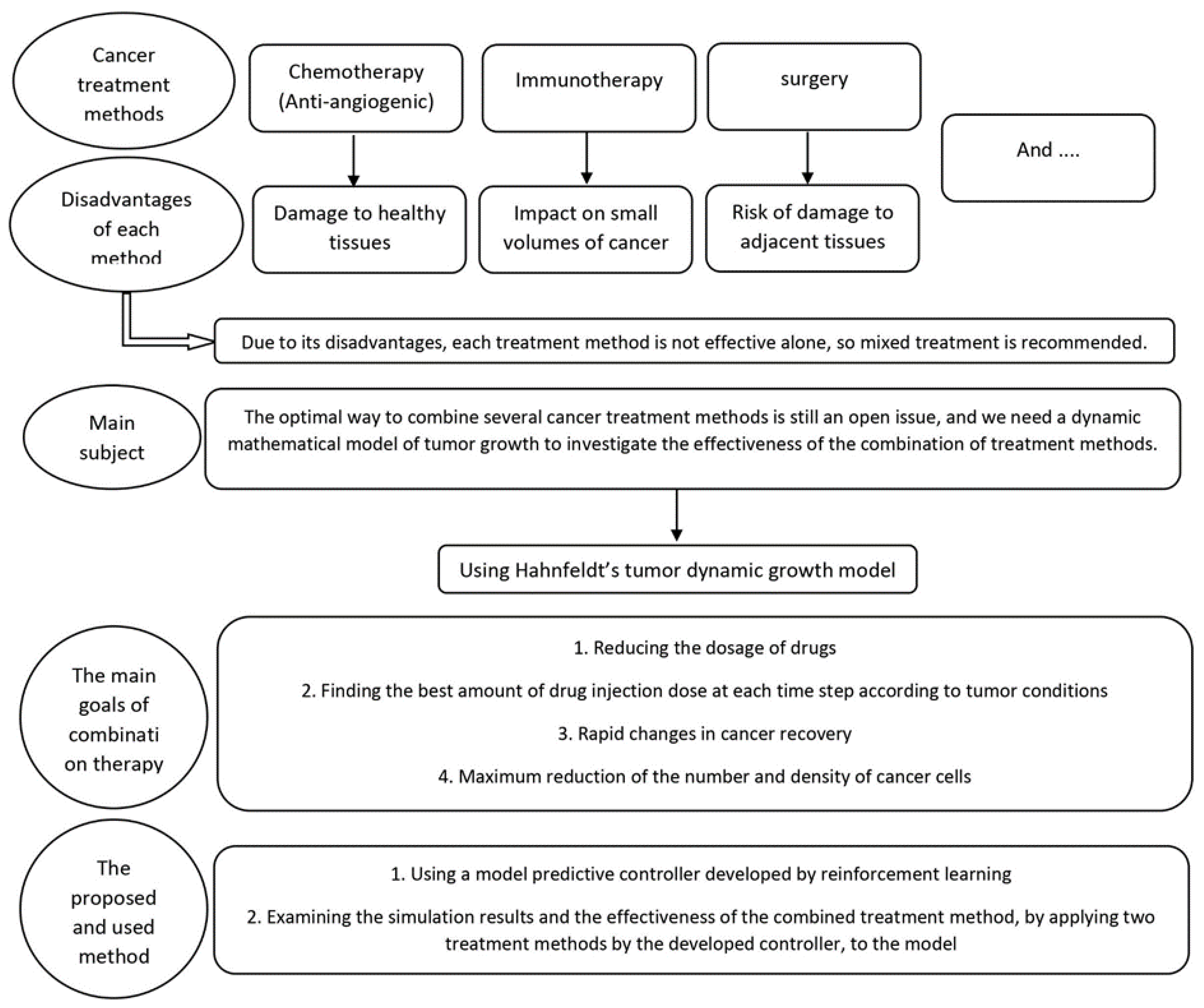
Figure 2.
MPC base diagram [21].
Figure 2.
MPC base diagram [21].
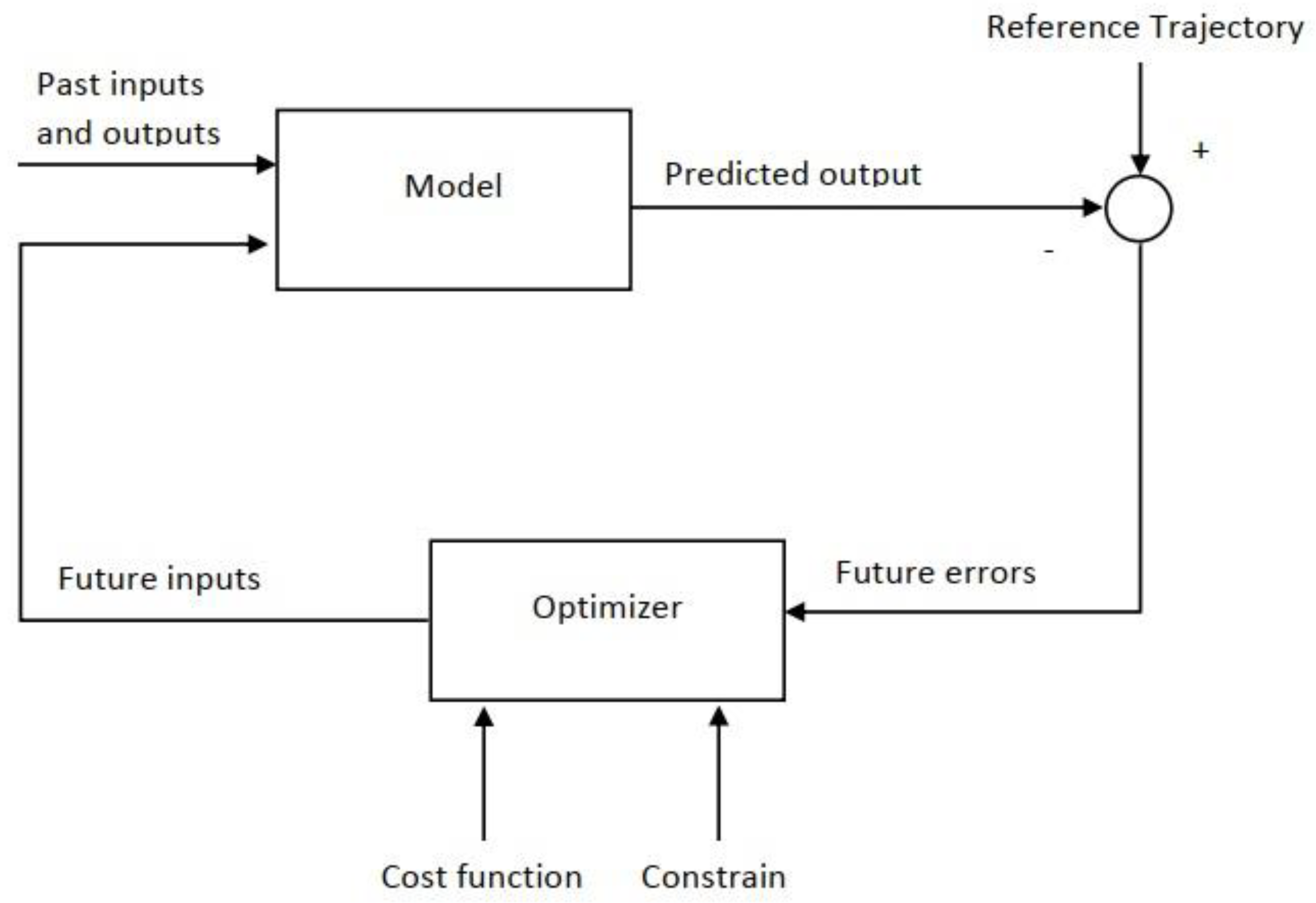
Figure 3.
Reinforcement learning schematic.
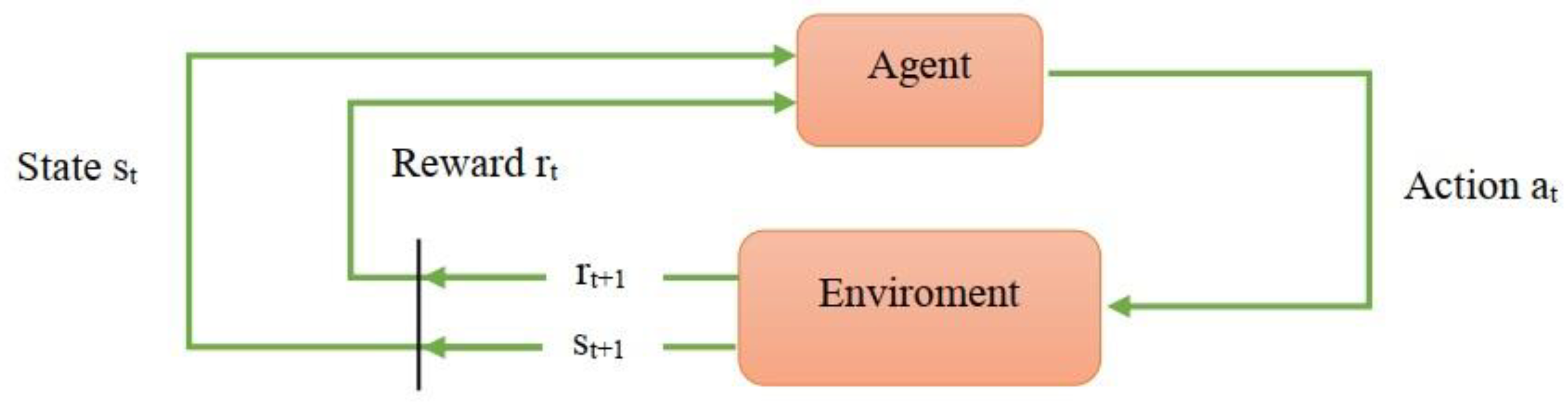
Figure 4.
The principles of Reinforcement Learning.
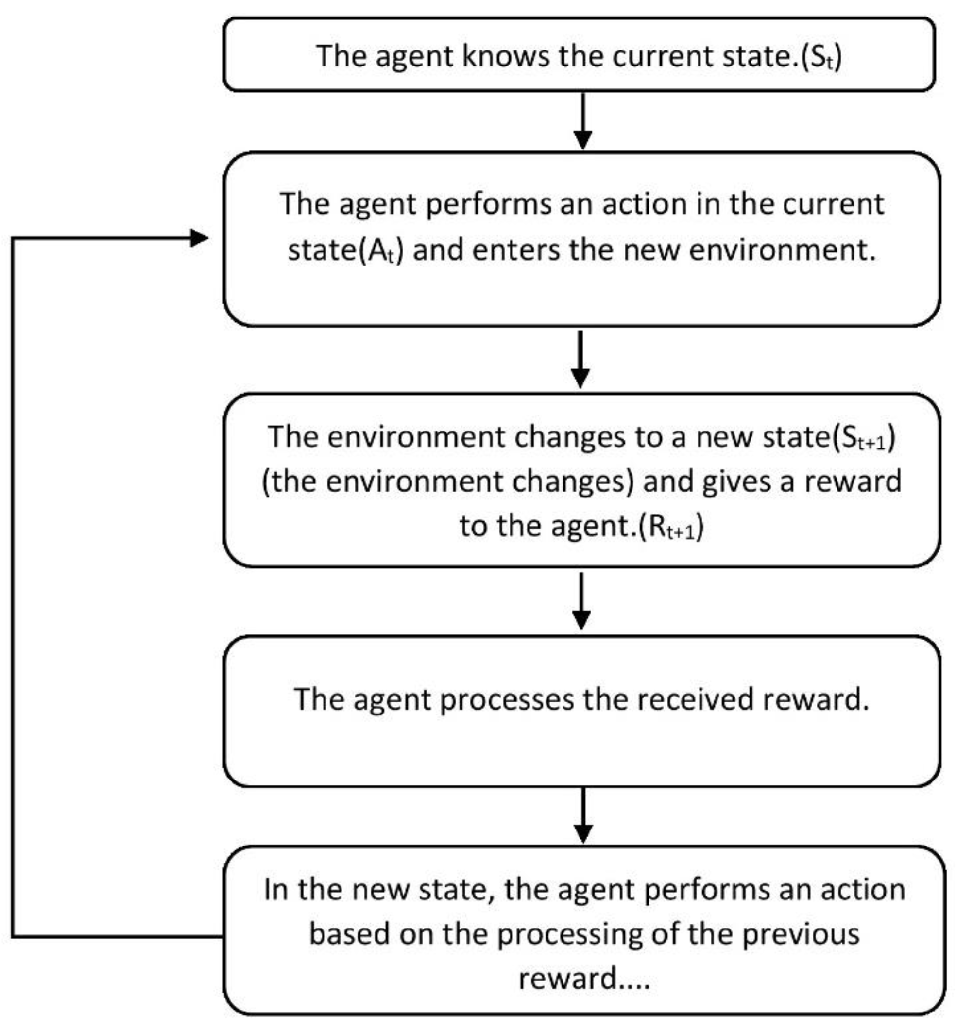
Figure 5.
The Markov Decision Process.
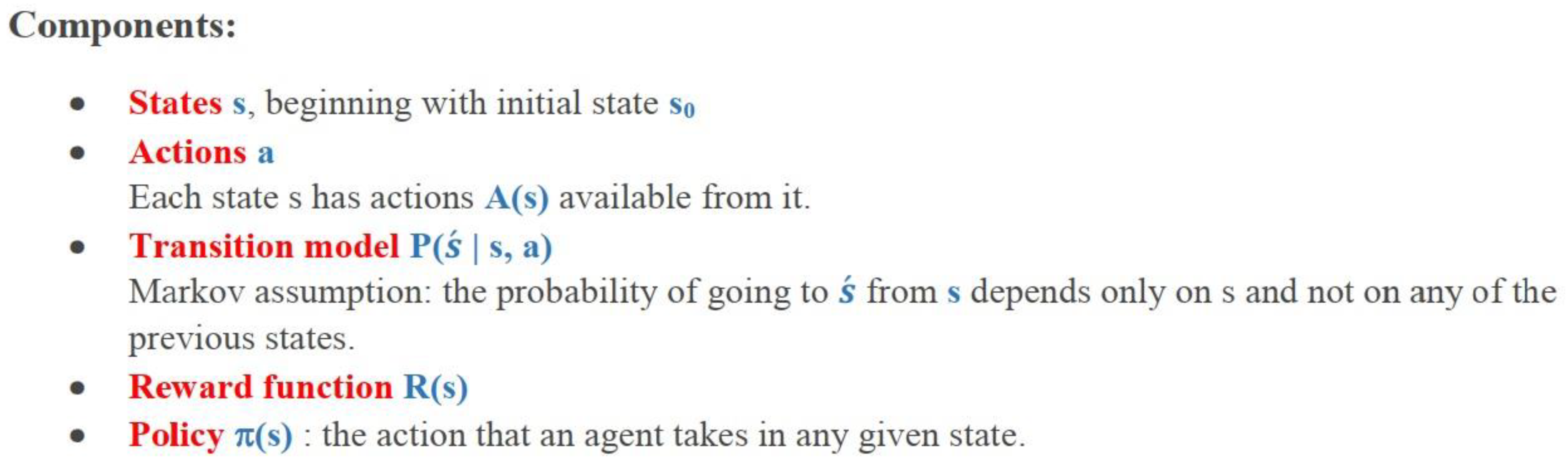
Figure 6.
Choose the action using ε−greedy policy.
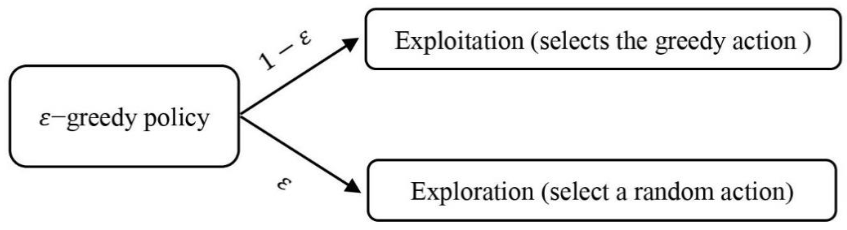
Figure 7.
The performance of the designed system components and their interaction with each other.
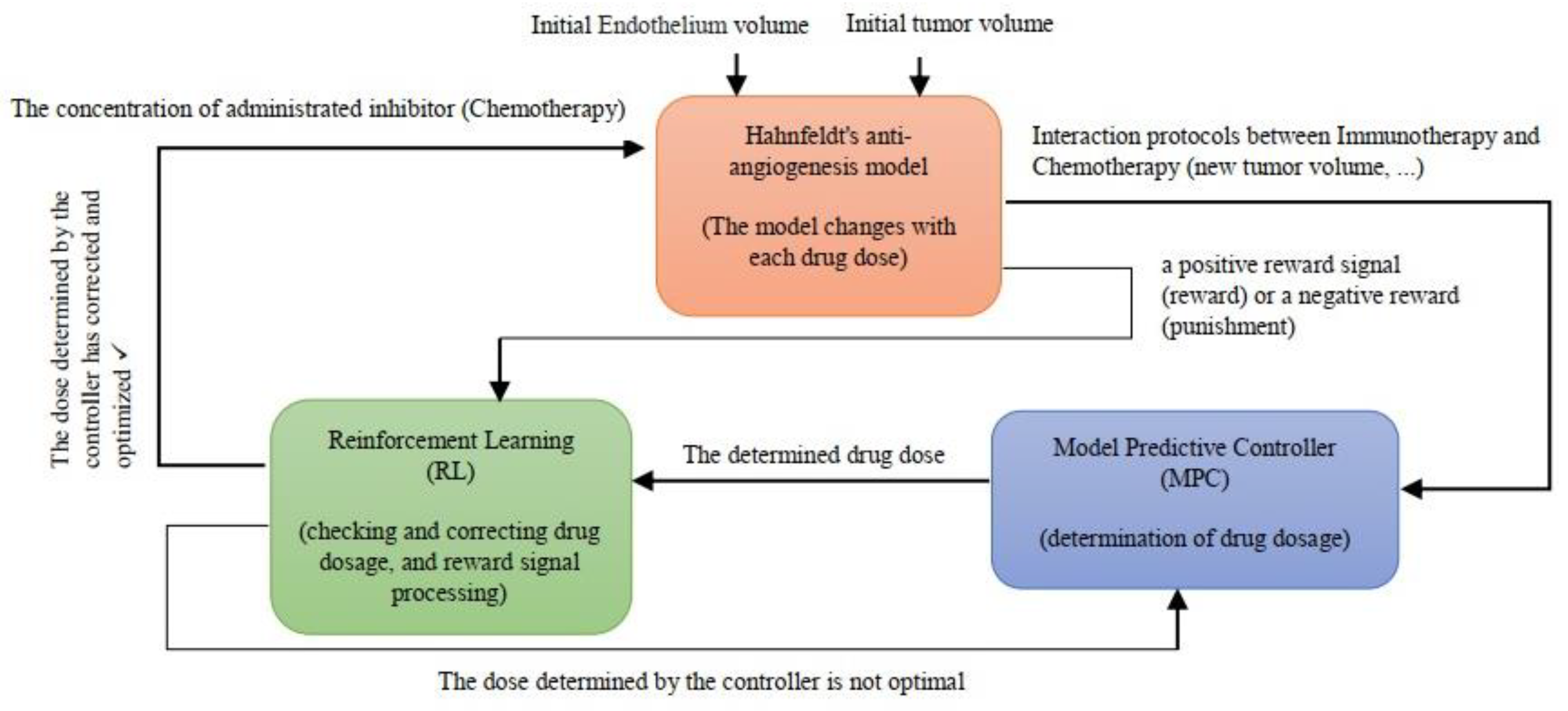
Figure 8.
The number of cells without applying a constraint by RL to the controller.
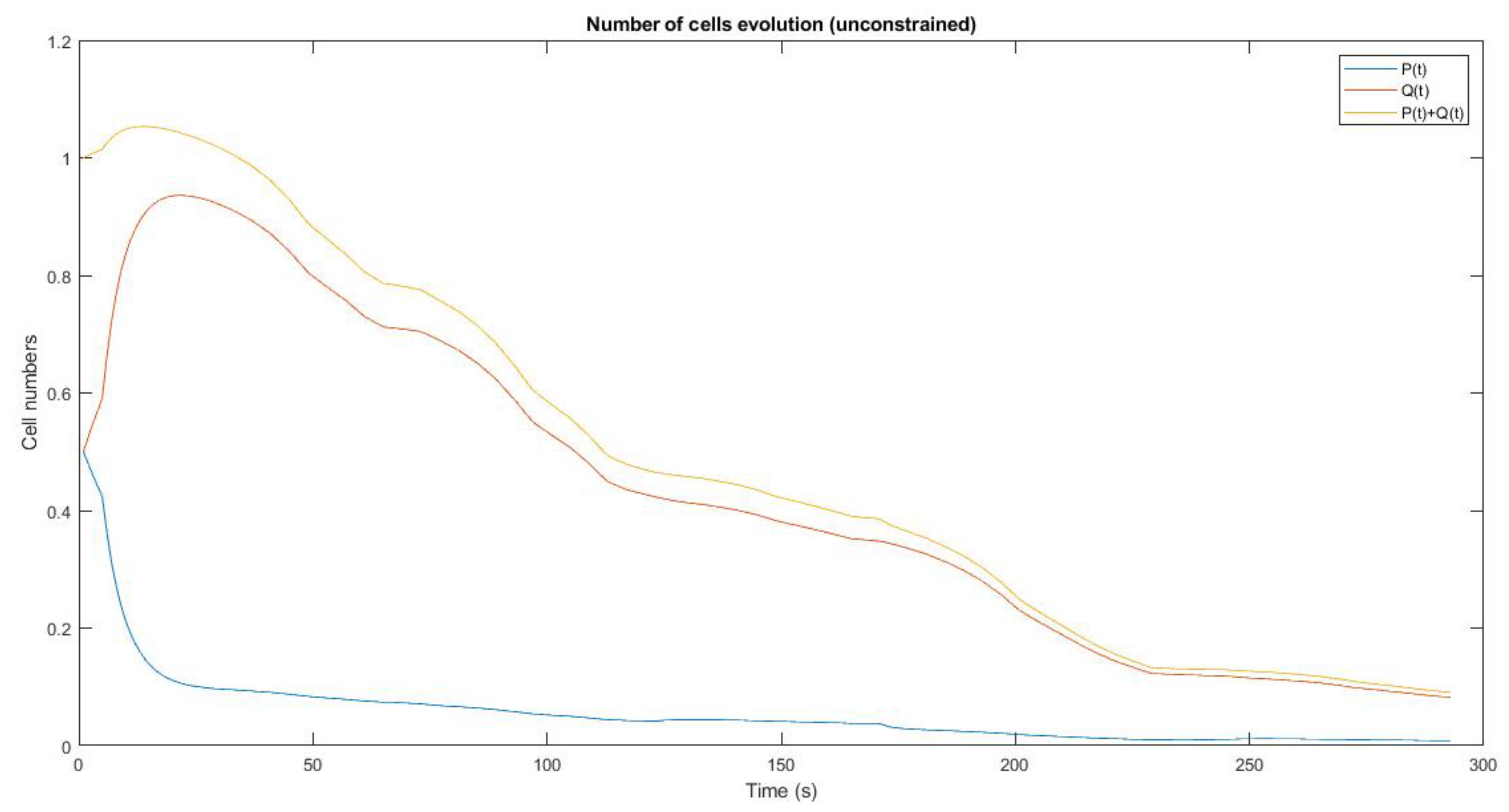
Figure 9.
The number of cells and optimal control sequence by using RL and without the initial conditions in different time steps.
Figure 9.
The number of cells and optimal control sequence by using RL and without the initial conditions in different time steps.
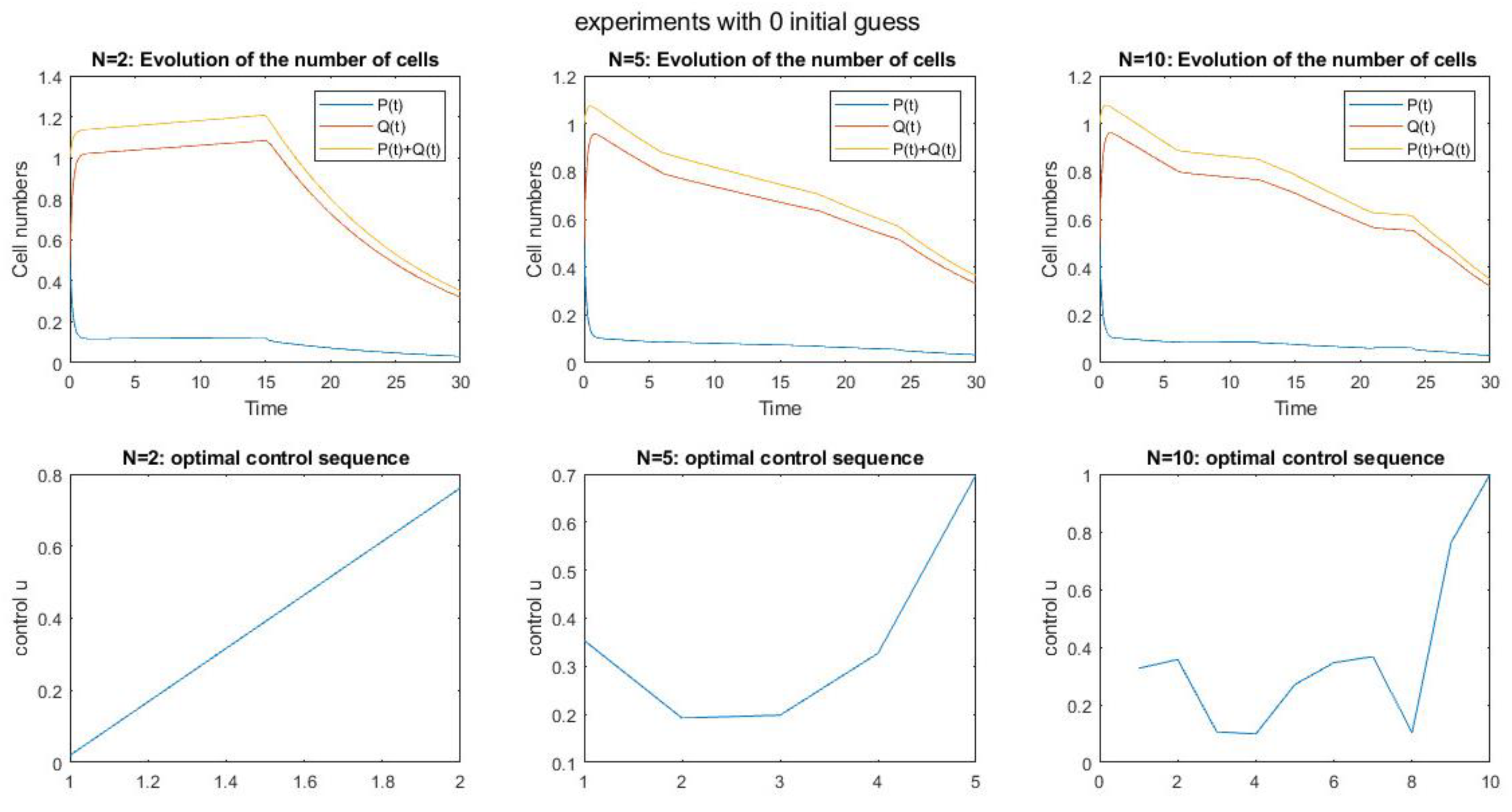
Figure 10.
The number of cells and optimal control sequence by using RL and with random initial conditions in different time steps.
Figure 10.
The number of cells and optimal control sequence by using RL and with random initial conditions in different time steps.
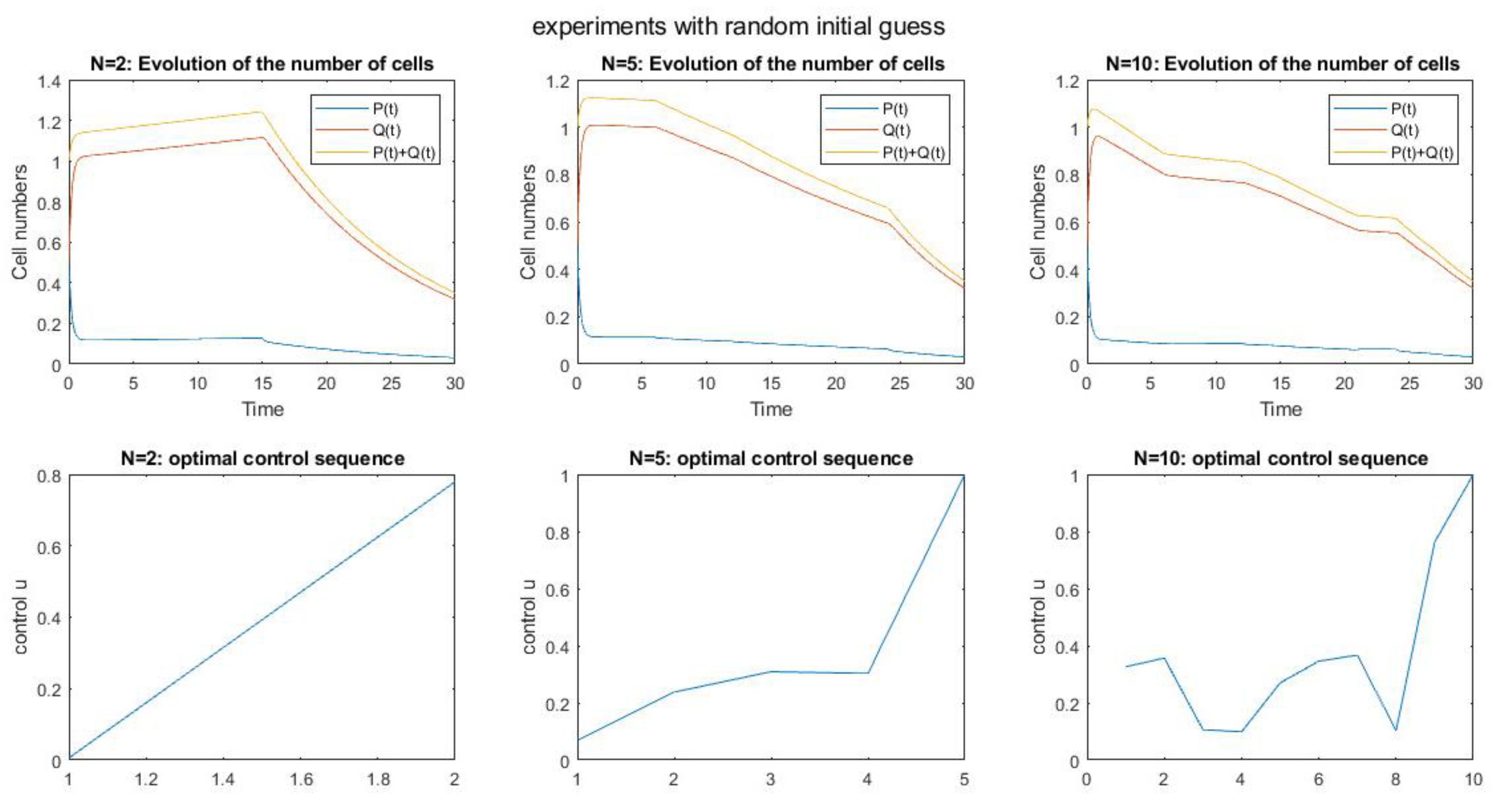

Table 1.
parameters value of dynamic system [18].
Table 1.
parameters value of dynamic system [18].
| Parameter | Value | Definition | Dimension |
|---|---|---|---|
| 0.192 | Tumor growth rate | 1/day | |
| 0 | Spontaneous loss of functional vasculature | 1/day | |
| 1.3 | clearance rate of inhibitor | 1/day | |
| b | 5.85 | stimulatory effect | 1/day |
| d | 0.0873 | inhibition effect of the tumor | 1/mm2.day |
| e | 0.66 | drug killing parameter | kg/mg.day |
Table 2.
The model parameters definitions [18].
Table 2.
The model parameters definitions [18].
| Parameter | Definition | Dimension |
|---|---|---|
| Tumor volume | mm3 | |
| Endothelial volume | mm3 | |
| Concentration of an administrated inhibitor | mg/kg | |
| The concentration of an administrated inhibitor | mg/kg | |
| Administrated inhibitor rate | mg/kg/day | |
| Tumor cells | 106 cells | |
| Immune competent density | Non-dimensional |
Table 3.
parameters value of MPC [10].
Table 3.
parameters value of MPC [10].
| Parameter | Value | Dimension | Definition |
|---|---|---|---|
| - | 106 cells | Tumor cells | |
| - | non-dimensional | Immune competent density | |
| 0.37451 | 1/day | Penalties |
Table 4.
The model parameters definitions of MPC [10].
Table 4.
The model parameters definitions of MPC [10].
| Parameter | Definition |
|---|---|
| Desired output | |
| The estimated output of the system at instant | |
| The prediction horizon | |
| Weighting matrices on output errors and is defined , | |
| Weighting matrices on control signals and is defined, | |
| Penalties on errors in tumor cells | |
| Penalties on immune competent density | |
| Penalties on | |
| Penalties on |
Table 5.
The MDP policy parameters and definitions.
| Parameter | Definition |
|---|---|
| A finite set of states | |
| A finite set of actions | |
| Current state () | |
| New state or environment ( | |
| An action () takes a state to | |
| The probability of transition to by taking an action in a state | |
| A state transition probability matrix | |
| The reward of taking an action in a state | |
| A reward function | |
| The discrete states in the set and | |
| The total number of states | |
| Elements of action set and | |
| The total number of actions | |
| The action-value function | |
| The expected sum of future rewards of taking a given actionin a state | |
| The optimal action-value function | |
| learning rate that affects the size of correction after each iteration () | |
| ζ | Discount factor which highlights the importance of the future rewards for values near to 1 and importance of immediate rewards for values near to zero. ( |
Table 6.
The ε−greedy policy parameters and definitions.
| Parameter | Definition |
|---|---|
| The desired tumor volume in | |
| Sampling time | |
| Time step | |
| The reward value | |
| Each state at the time step |
Disclaimer/Publisher’s Note: The statements, opinions and data contained in all publications are solely those of the individual author(s) and contributor(s) and not of MDPI and/or the editor(s). MDPI and/or the editor(s) disclaim responsibility for any injury to people or property resulting from any ideas, methods, instructions or products referred to in the content. |
© 2025 by the authors. Licensee MDPI, Basel, Switzerland. This article is an open access article distributed under the terms and conditions of the Creative Commons Attribution (CC BY) license (http://creativecommons.org/licenses/by/4.0/).
Copyright: This open access article is published under a Creative Commons CC BY 4.0 license, which permit the free download, distribution, and reuse, provided that the author and preprint are cited in any reuse.


