Submitted:
03 February 2025
Posted:
05 February 2025
Read the latest preprint version here
Abstract
Accurate identification of druggable pockets is essential for structure-based drug design. However, most pocket-identification algorithms prioritize their geometric properties over downstream docking performance. To address this limitation, we developed RAPID-Net, a pocket-finding algorithm for seamless integration with docking workflows. When guiding AutoDock Vina, RAPID-Net outperforms DiffBindFR on the PoseBusters benchmark and enables blind docking on large proteins that AlphaFold 3 cannot process as a whole. Furthermore, RAPID-Net surpasses PUResNet and Kalasanty in docking accuracy and pocket-ligand intersection rates across diverse datasets, including PoseBusters, Astex Diverse Set, BU48, and Coach420. When accuracy is evaluated as ``at least one correct pose in the ensemble'', RAPID-Net outperforms AlphaFold 3 on the PoseBusters benchmark, suggesting that our approach can be further improved with a suitable pose reweighting tool offering a cost-effective and competitive alternative to AlphaFold 3 for docking. Finally, using several therapeutically relevant examples, we demonstrate the ability of RAPID-Net to identify remote functional sites, highlighting its potential to facilitate the development of innovative therapeutics.
Keywords:
Protein–ligand interactions
; Blind docking
; Binding pocket prediction
; Soft mask segmentation
; Deep residual network
; Convolutional Neural Network
1. Introduction and Problem Statement
Molecular docking is the computational problem of predicting the most favorable ligand binding poses in a protein-ligand complex, given the experimentally determined or computer-simulated protein structure and the initial conformation of the ligand [1]. It plays a key role in drug development, typically following target identification when the biological molecule responsible for a disease is identified and validated as a therapeutic target [2]. Once the target is identified, molecular docking is used for structure-based drug discovery and development [3,4] to identify and optimize potential lead compounds [5,6]. The docking results can guide virtual screening workflows, enabling the selection of promising candidates from vast chemical libraries [7,8]. This process helps to determine whether a compound has potential for drug development [9]. By significantly improving the speed and efficiency of early drug discovery, molecular docking reduces the time and costs associated with the development of new therapeutics [10].
Typical protein-ligand docking pipelines rely on users specifying the binding pocket, and docking programs such as AutoDock Vina [11,12], GOLD [13], and Glide [14], use grids to confine their search to known or hypothesized protein’s interaction sites. However, in the absence of such information – in “blind” or binding-site-agnostic settings – protein-ligand docking becomes significantly more difficult [15], as the docking algorithm must scan the entire protein surface, dramatically increasing the computational complexity. Traditional blind docking methods often rely on extensive sampling to explore potential binding sites across the whole protein, but this approach is computationally and time-intensive, making it impractical for large-scale virtual screening tasks [16,17].
With the advent of advanced protein structure prediction methods [18]–including AlphaFold [19], ColabFold [20], OpenFold [21], and RosettaFold [22]–the number of generated protein structures has surged, often without any corresponding ligand information. Meanwhile, only about of human coding genes currently serve as commercial drug targets, leaving a vast array of disease-related targets unexplored [23]. Despite this immense potential, most new drug research and development remains focused on a limited set of well-established targets, underscoring the urgent need for novel druggable targets [24]. As more proteins lacking known binding pocket information are considered in drug discovery [25], the demand for ligand docking approaches that do not rely on prior knowledge of the binding site has grown significantly, highlighting the necessity for binding-site-agnostic methods.
At the same time, many existing protein binding site identification algorithms are evaluated primarily on the geometric properties of their predicted pockets [26], rather than on how accurately they guide subsequent ligand docking. In this work, our primary objective is to develop a pocket-finding algorithm that can be readily integrated with standard docking software and provide accurate, efficient guidance in binding-site-agnostic settings. We evaluate its performance both in terms of docking accuracy–using AutoDock Vina 1.2.5 [12]–and the geometric characteristics of the generated pockets.
In terms of underlying pocket prediction function, existing algorithms can be broadly classified into classical and Machine Learning (ML)-driven approaches [26]. Classical methods rely on expert-defined rules or heuristics to detect pockets, whereas ML-driven algorithms learn to extract features from protein data without explicit human instructions. In this work, we adopt the definition of Machine Learning by François Chollet as “the effort to automate intellectual tasks normally performed by humans” [27]. From this perspective, the main objective of an ML framework is to unveil a meaningful data representation that allows pocket-prediction rules to emerge automatically, rather than being manually hardcoded.
Furthermore, “Deep Learning (DL) is a specific subfield of Machine Learning: a new take on learning representations from data that puts an emphasis on learning successive layers of increasingly meaningful representations” [27]. In the context of pocket identification in our study, these layers of data representations are realized through Deep Neural Networks (DNNs). Finally, in contrast to DL, so-called “shallow” learning approaches typically employ only one or a small number of consecutive data representation layers [27].
In the following Sections, we describe our DL model for pocket identification, named RAPID-Net (ReLU Activated Pocket Identification for Docking). We tested RAPID-Net on various benchmarks to demonstrate its efficiency and analyzed its predictions on several therapeutically important proteins. In Section 2, we discuss the architecture and design rationale behind our model. In Section 3, we present the RAPID-Net training pipeline, highlighting its key differences from existing approaches, including the use of ReLU activation in the last layer of the network to operate on a “soft” rather than binary labels. Using the RAPID-Net model developed in Section 2 and Section 3, in Section 4 we integrate it into a docking protocol that is subsequently used for docking. In Section 5, we describe the evaluation metrics used to assess the quality of the model’s predictions. Section 6 and Section 7 report docking results on the PoseBusters [28] and Astex Diverse Set [29] datasets, respectively. For completeness and to provide a direct side-by-side comparison with existing pocket prediction algorithms, Section 8 evaluates the geometric characteristics of predicted pockets on the Coach420 [30] and BU48 [31] datasets. To demonstrate the ability of RAPID-Net to identify distant binding sites, Section 9 analyzes its predictions for several therapeutically important proteins with known distal sites. Finally, in Section 10, we reach our conclusions and outline the potential directions for future work.
Figure 1.
Alpha-spheres predicted by FPocket and the majority-voted pocket predicted by our RAPID-Net model for the ABHD5 protein.
Figure 1.
Alpha-spheres predicted by FPocket and the majority-voted pocket predicted by our RAPID-Net model for the ABHD5 protein.
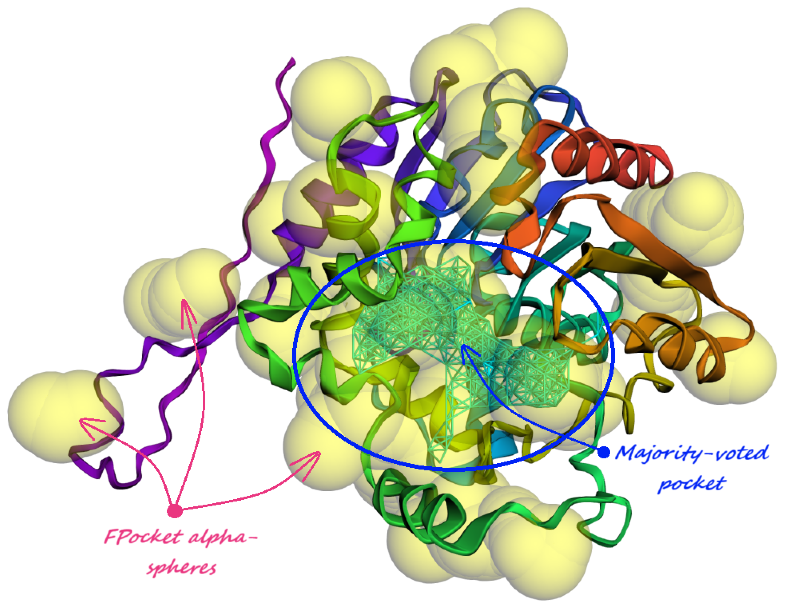
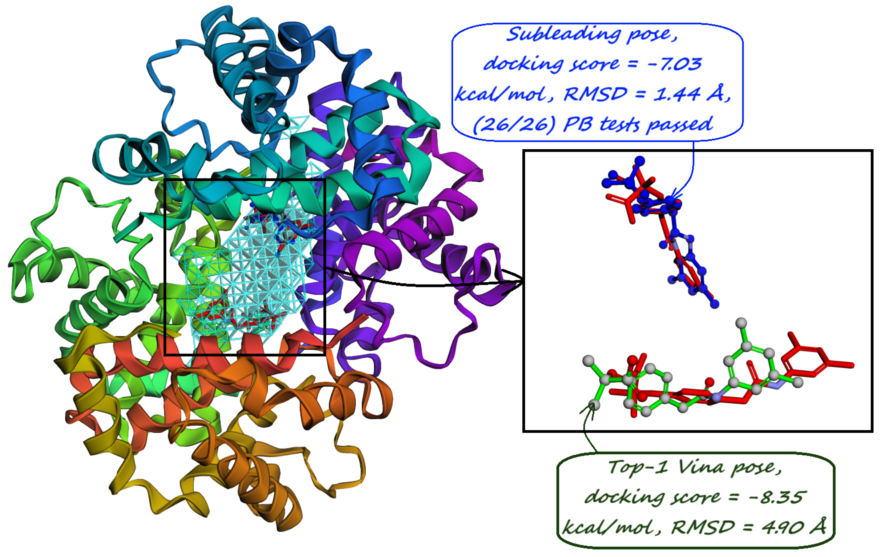
Figure 2.
8DP2 protein structure from the PoseBusters dataset [28]. The Top-1 Vina pose is docked in a predicted sub-pocket devoid of true ligand binding pose, while the subleading pose correctly occupies a second predicted sub-pocket and passes all validation tests.
Figure 2.
8DP2 protein structure from the PoseBusters dataset [28]. The Top-1 Vina pose is docked in a predicted sub-pocket devoid of true ligand binding pose, while the subleading pose correctly occupies a second predicted sub-pocket and passes all validation tests.
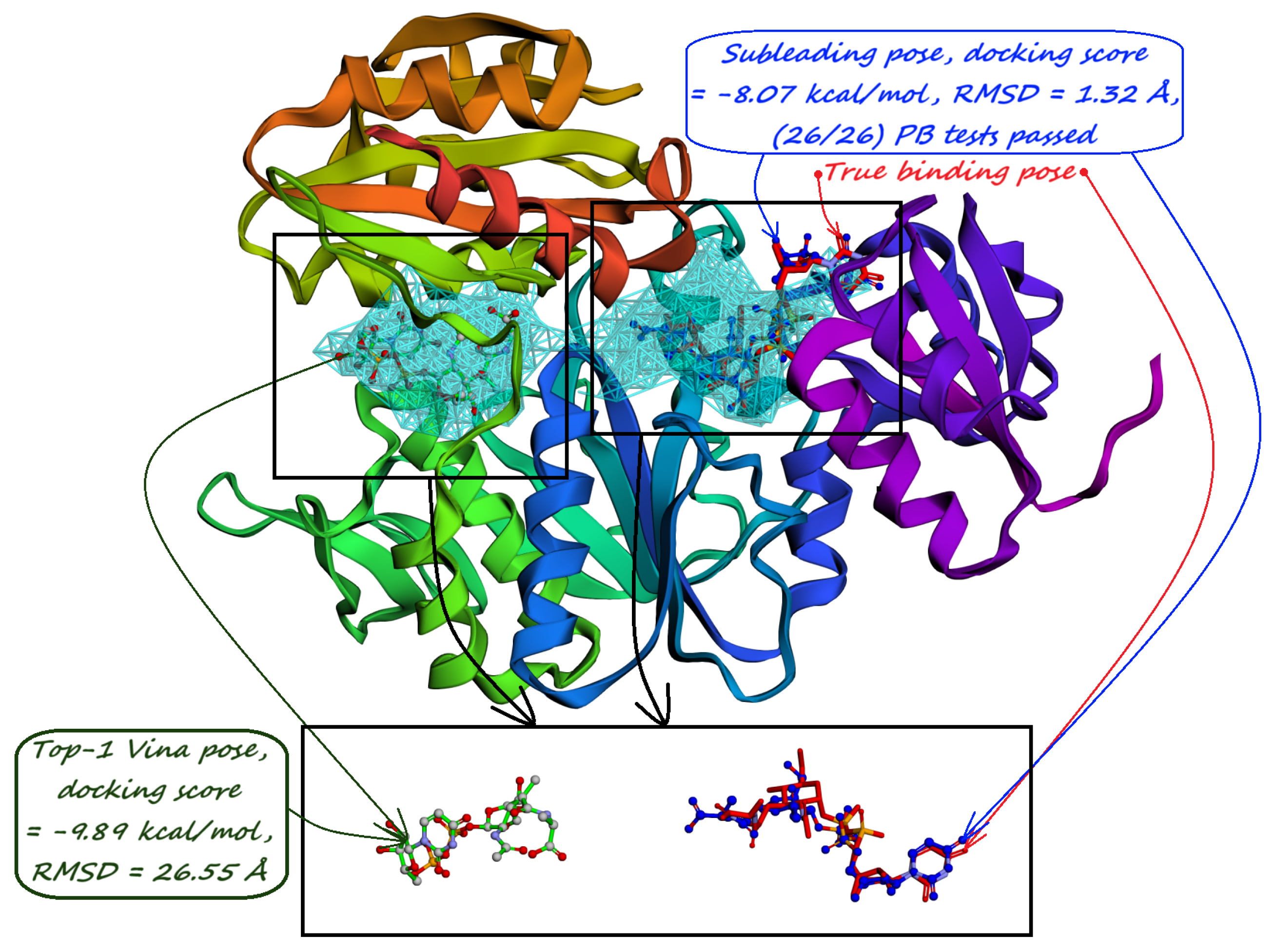
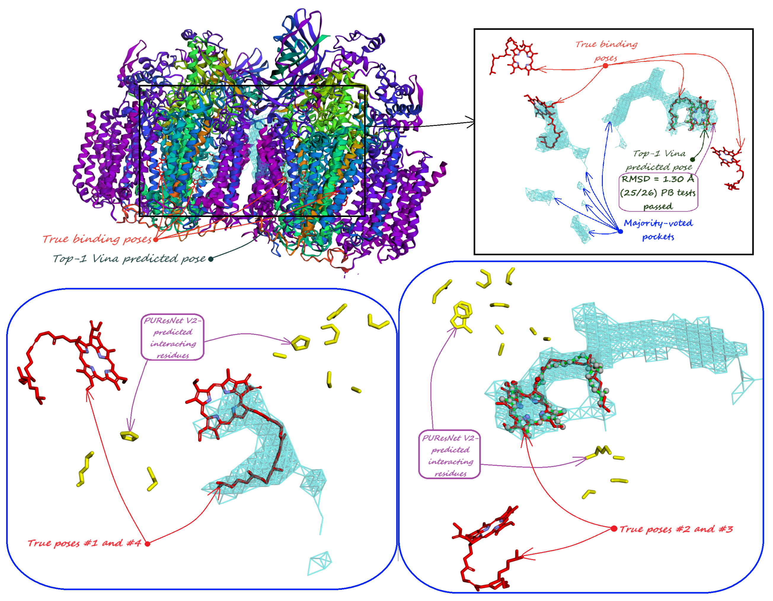
Figure 3.
For the 8F4J protein structure from the PoseBusters [28] dataset, our docking approach passes the RMSD test and 25/26 PoseBusters [28] validation checks, outperforming AlphaFold 3 [32], which cannot process the structure as a whole. Unlike residue-focused methods such as PUResNet V2 [33], which produce complex predictions that are difficult to interpret, our approach offers clear, plug-and-play guidance for docking grid selection, as illustrated in the bottom panel.
2. Design Rationale Behind Our Model
When predicting likely binding pockets, there is a well-known trade-off between precision and recall. A recent evaluation of pocket prediction methods based on the geometrical properties of their predicted pockets [26] highlights this trade-off. Currently available ML methods such as VN-EGNN [34], GrASP [35], and PUResNet [36] achieve high precision (over 90%), but they systematically predict a small number of pockets, leading to low recall. As [26] points out, generating multiple predictions, some of which may be false positives, is often more useful than potentially missing viable binding sites.
To address this shortcoming and mitigate low recall, we develop RAPID-Net as an ensemble-based model to improve the stability of prediction accuracy and coverage of potential binding sites. RAPID-Net consists of five independently trained model replicas to aggregate results and increase the reliability of its predictions. For subsequent docking, RAPID-Net returns two types of pockets:
- Majority-voted pockets: Consisting of voxels predicted by at least 3 out of 5 ensemble models, for high-confidence predictions.
- Minority-reported pockets: Consisting of voxels predicted by at least 1 out of 5 ensemble models, increasing the overall recall.
As demonstrated on diverse benchmark datasets in the following Sections, including PoseBusters [28], Astex Diverse Set [29], Coach420 [30], and BU48 [31], the proposed ensemble-based approach yields more stable and reliable performance compared to current ML-driven pocket predictors, both considering the majority-voted and minority-reported pockets.
For instance, consider the 8DP2 protein from the PoseBusters [28] dataset, illustrated in Figure 2. RAPID-Net predicts two majority-voted sub-pockets connected by a link. However, because no ligand binding occurs in one of these sub-pockets, it constitutes a false positive. By contrast, one of the subleading poses binds within the second predicted sub-pocket and passes all tests. This example demonstrates RAPID-Net’s ability to balance accuracy and recall, providing a comprehensive and robust pocket prediction framework for complex docking tasks. Furthermore, as shown in the following Sections, the minority-reported pockets predicted by our model are often shallow pockets corresponding to secondary binding sites, in contrast to the more prominent majority-voted pockets.
On the other hand, FPocket [37] typically predicts many, often overlapping alpha-spheres, making it difficult or even impossible to segment the protein surface clearly. FPocket [37] can place alpha spheres in adjacent but distinct pockets, introducing ambiguity in the definition of distinct docking regions. As an illustration, for the ABHD5 protein structure obtained from AlphaFold [19] shown in Figure 1, the majority-voted pocket predicted by our model forms a compact clearly defined region. If FPocket [37] was used in the docking pipeline instead, nearly the entire protein surface would need to be included, drastically increasing computational costs.
The drawbacks of overly large search grids can be illustrated by the 8F4J protein structure from the PoseBusters [28] (PB) dataset, shown in the top panel of Figure 3. Even advanced docking platforms such as AlphaFold 3 [32], which incorporate FPocket [37] to locate potential docking sites, cannot process the entire 8F4J protein as a whole: “Another PDB entry (8F4J) was too large to inference the entire system (over 5,120 tokens), so we included only protein chains within of the ligand of interest.” [32]. In contrast, as shown in Figure 3 and discussed further in the text, the RAPID-Net guidance allows AutoDock Vina [11,12]to generate a pose passing the test and satisfy 25/26 PoseBusters (PB) tests.
Types of outputs from pocket predictors. The type of output produced by pocket predictors can be divided into three main categories.
Kalasanty [38] and PUResNet V11 [36] both detect potential ligand-binding pockets using a voxel-based representation, where each voxel is in size.
In contrast, PRANK [39] and DeepPocket [40] reweight the alpha-spheres identified by the rule-based FPocket [37] algorithm. As a result, these methods inherit FPocket’s initial search space and any associated cascading errors. Moreover, alpha-sphere-based approaches may lack sufficient granularity and can struggle to capture subtle variations among binding sites.
GrASP [35], IF-SitePred [41], VN-EGNN [34], and PUResNetV2 [33] provide predictions of potential ligand interactions at the residue level. Although these predictions can reveal important binding details, they are less suitable for docking workflows that require a well-defined three-dimensional region for accurate ligand placement and orientation. By precisely defining these regions, the computational search space is reduced as docking is restricted to reasonable binding pockets. As illustrated in the bottom panel of Figure 3, residue-level predictions can be difficult to interpret when defining a reasonable search grid.
Although some studies reweight residues to guide blind docking [42], and others [25] employ voxelized pocket prediction models–such as PUResNet [36]–in tandem with AutoDock Vina [12], our work focuses on developing a voxel-based cavity prediction model that seamlessly integrates into the docking pipeline. This voxel-based approach not only provides well-defined search regions but also facilitates a more modular and interpretable workflow compared to less structured docking strategies, as illustrated in Figure 5 and discussed further in Section 4.
Furthermore, as discussed in Section 6, improving the accuracy of pocket identification directly improves docking results. In particular, AutoDock Vina [12], guided by our pocket predictor, outperforms the state-of-the-art DiffBindFR [43] docking tool, which otherwise scans the entire protein surface in “blind” settings.
Our model architecture. Figure 4 depicts the architecture of our proposed RAPID-Net model, which is similar to U-Net [44] with encoder and decoder branches. However, we implement several notable adaptations.
First, we include residual connections only in the encoder part of the model, as our experiments show that they are highly beneficial there, but lead to overfitting if included in the decoder. This approach differs from Kalasanty [38], which omits residual blocks altogether [45], and PUResNet [36], which uses them throughout the network.
Second, although the standard SE-ResNet [46] architecture typically includes attention blocks at multiple layers, studies on breast-cancer imaging [47] and Raman spectra classification [48] have shown that using a single attention block can be highly effective while mitigating overfitting. Our experiments similarly suggest that in inherently noisy datasets, adding too many attention modules can amplify noise and degrade performance.
As we demonstrate in the following Sections, adopting a moderate level of attention, limiting residual connections, and incorporating a modified loss function significantly improves performance compared to earlier models.
Figure 4.
Schematic representation of RAPID-Net (ReLU-Activated Pocket Identification for Docking). Key improvements that distinguish RAPID-Net from previous approaches include a ReLU activation in the final layer, the usage of a soft dice loss function, including a single SE-attention block, and removing redundant residual connections.
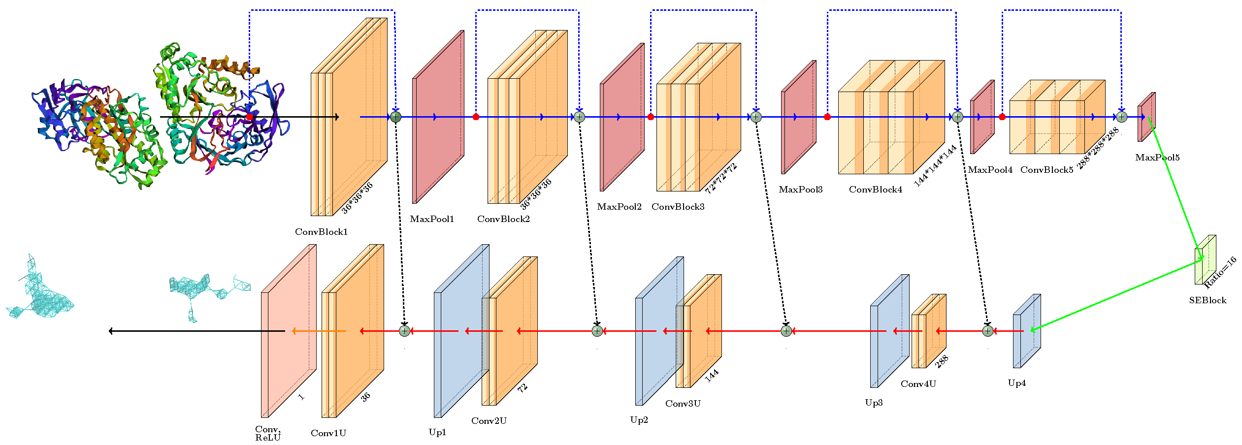
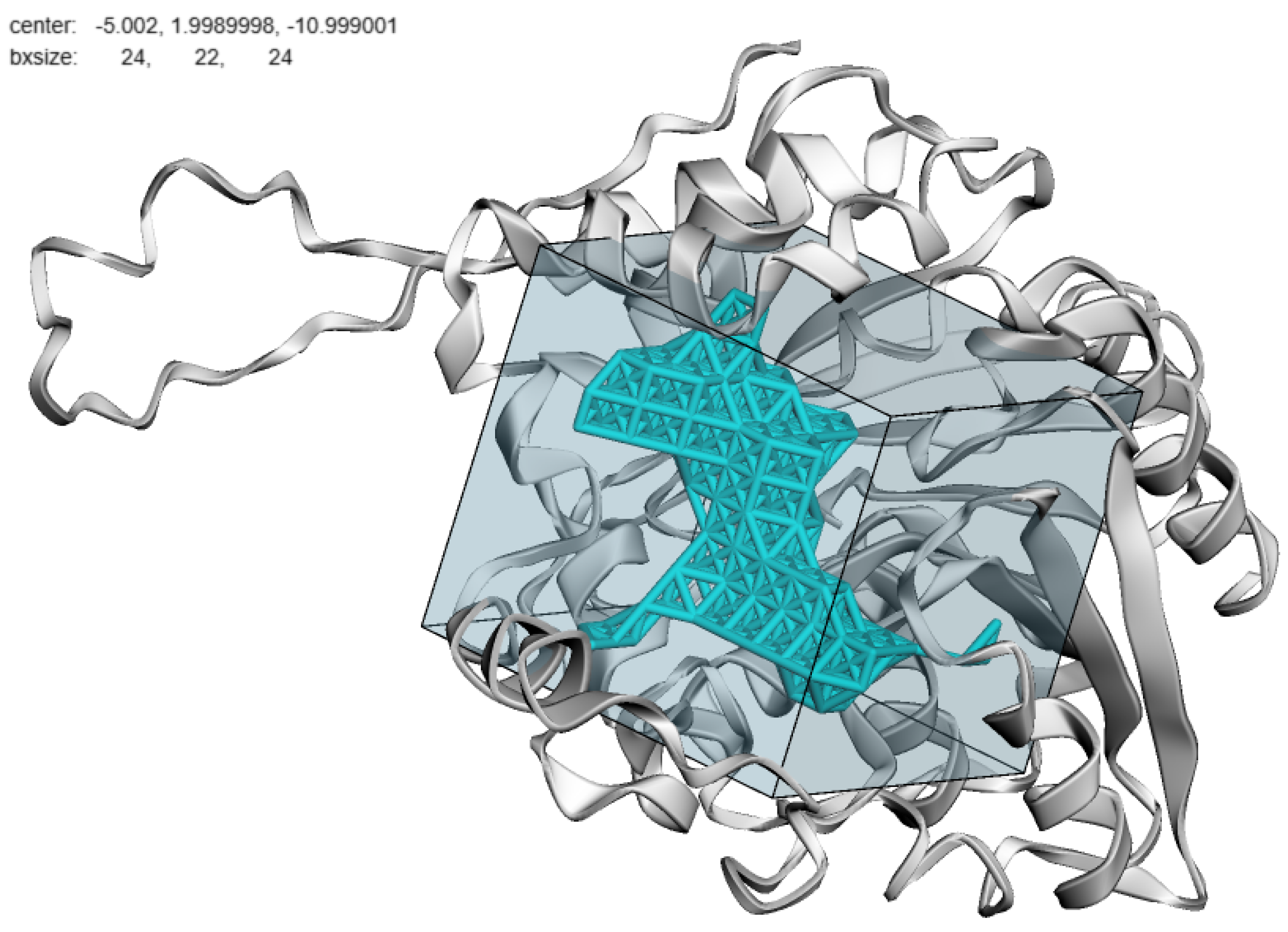
Figure 5.
Majority-voted pocket predicted by RAPID-Net and its corresponding search grid with 2 Å threshold for ABHD5 protein.
Figure 5.
Majority-voted pocket predicted by RAPID-Net and its corresponding search grid with 2 Å threshold for ABHD5 protein.
3. Model Training and Inference Pipeline
We trained our model using the sc-PDB [49] dataset, which contains protein structures with annotated binding sites. In this dataset, cavities are defined using VolSite [50], which maps the pharmacophore properties of nearby protein atoms onto a three-dimensional grid. This method assumes that ligand-induced conformational changes remain relatively small [51], treating each cavity atom as a “pseudoatom” to denote an interaction point rather than a physical atom.
Following [36], we used a curated subset of sc-PDB [49] in which redundant protein structures were filtered out based on their Tanimoto index [52]. Each protein structure was then placed in a grid, with each voxel corresponding to a unit cell. We extracted 18 features per voxel using the tfbio [53] package to provide a representation of the protein environment for the model training.
In contrast to previous studies, we apply the medical image segmentation practices [54,55,56] to perform soft segmentation of ligand-binding pockets, rather than treating it as a strict binary classification problem. In Kalasanty [38] and PUResNet [36], each voxel is considered part of a binding pocket if it contains at least one cavity pseudoatom. The number of pseudoatoms per voxel is then clipped to the range , and the model is trained with a Dice loss function as part of a binary classification task:
where and represent the binary masks of the true and predicted pockets, respectively, ∩ indicates their intersection, and and denote the number of occupied voxels in the true and predicted masks, respectively.
Recently, PUResNet V2 [33] sought to improve performance by replacing the Dice loss function with a focal loss [57]. However, our extensive experiments indicate that adopting a “soft” approach [54,55,56] is better suited in this context. In contrast to the binary “yes/no” classification of occupied voxels, the density of pseudoatoms serves as an indicator of the proximity of a voxel to the interior or boundary of a pocket. Higher densities typically occur near polar or charged residues and ligand functional groups, whereas lower densities are often associated with hydrophobic regions.
Drawing inspiration from medical image segmentation methods [54,55,56], we replace the sigmoid output in the final layer with a ReLU [58] (hence the name of our model, ReLU Activated Pocket Identification for Docking, RAPID-Net):
For the model training, we also replace the conventional Dice loss in Eq. 1 with its “soft” variant:
Several ways of implementing the “soft” Dice loss have been proposed [55,56], but we found that this simplest version, based on the norm, works best.
To mitigate class imbalance, as the number of non-interacting voxels sharply exceeds the number of interacting ones, we applied class reweighting using scikit-learn [59]. During inference, a voxel is classified as part of a binding pocket if the model output exceeds . When ensembling five models, we apply morphological closing using the binary_closing function from the scipy.ndimage package [60] to mitigate sparsity in the predicted pocket regions across model replicas.
Unlike previous approaches that use cavity6.mol2 labels [36,38], we train our model with threshold-less pocket labels (cavityALL.mol2). In cavity6.mol2, annotations are restricted to regions within of the ligand’s heavy atoms [49], potentially overlooking distal functional regions such as allosteric pockets, exosites, or flexible loops. These sites can critically influence drug binding and resistance, making them key therapeutic targets. Secondary binding sites, which often lie beyond the boundary, mediate interactions with larger substrates or cofactors and help position them within the catalytic pocket, as further discussed in Section 9. By adopting threshold-less labels, our model identifies both catalytic and more distant sites, thereby improving predictions for proteins that contain such secondary binding regions.
This approach also makes the Distance Center Center (DCC) metric, which was previously used to evaluate Kalasanty [38] and PUResNet [36], less relevant. DCC defines the distance between the geometrical center of the predicted pocket and the true ligand binding pose, but “tunnels” can extend from the primary binding pocket to distal residues that lie far from the ligand but have significant therapeutic implications (see Section 9 for examples). Furthermore, the threshold-less pocket definition is less sensitive to the ligand size, thereby improving the generalizability of our model.
4. Docking Protocol and its Rationale
For each predicted pocket, we define the center of the search grid as the average of the maximum and minimum x, y, and z coordinates of all pseudoatoms in the pocket:
where and are the maximum and minimum coordinates, respectively. The grid dimensions are then given by:
Figure 5 illustrates this setup for the majority-voted pocket in the ABHD5 protein with a threshold value of 2 Å.
For each majority-voted pocket, we generate search grids with thresholds of and . For minority-reported pockets, we use thresholds of , , , and . This strategy accounts for large ligands, such as those in the PoseBusters [28] dataset, which may extend beyond the predicted pockets, and also reduces potential inaccuracies in our model’s pocket predictions.
As an example, Figure 6 shows the 8FAV protein from the PoseBusters dataset [28], where none of the predicted pockets overlap with one of the true ligand binding poses. However, the docking still succeeds because the expanded search grid thresholds encompass the true binding site. This case demonstrates how geometry-based evaluation metrics, such as those in [26], can overlook the practical success of docking, even if the pocket predictions are imperfect.
To demonstrate that the accuracy of our model is primarily a result of architectural and training improvements–not merely ensembling–we also provide single-model predictions from Kalasanty [38], PUResNet [36], and individual RAPID-Net runs. Similarly, for each predicted pocket, we generate grids with , , , and thresholds.
5. Test Benchmarks and Evaluation Metrics
We evaluate docking performance as the percentage of Top-1 Vina poses with a root mean square deviation (RMSD) below 2 Å between the predicted and one of the true ligand poses if multiple true poses are available. RMSD is calculated as:
where N is the number of ligand atoms, and are positions of the i-th atom in the true and predicted poses, respectively, and is the Euclidean norm. RMSD is computed using the CalcRMS function in RDKit [61].
Docking methods like AutoDock Vina [12] balance speed and accuracy [62], utilizing “fast and dirty” scoring functions. A common strategy to enhance their accuracy is to generate an ensemble of potential poses and then identify the best pose among them using more accurate scoring tools, for example [63,64]. Fast scoring functions enable the efficient exploration of numerous poses, while more accurate methods are reserved for refinement and final pose selection. To account for this approach, we also compute the ensemble RMSD accuracy as “at least one pose in the ensemble is correct”, highlighting the potential gains from precise rescoring. Since our primary focus is on improving pocket identification rather than developing new rescoring functions, we defer such work to the future. Our goal here is to illustrate the potential of our method when combined with an appropriate rescoring tool.
Additionally, we evaluate the PB-success rate, defined as the percentage of poses with Å that pass all 26/26 chemical validity checks defined by PoseBusters [28].
Finally, similarly to [36], we compute the Pocket-Ligand Intersection (PLI) score to quantify the proportion of ligand atoms residing within the predicted pocket. Unlike [36], which computes a voxel-based intersection, we measure the average fraction of ligand heavy atoms located within 5 Å of at least one pocket pseudoatom, yielding a more intuitive metric:
where is the number of ligand heavy atoms within 5 Å of any pocket pseudoatom, and is the total number of heavy atoms in the ligand.
However, unlike [36], we compute this ratio for all protein-ligand pairs in the dataset rather than restricting it to cases where the ligand is centered within of the pocket center. If no pockets are predicted, the PLI is set to zero. When a protein has multiple predicted pockets or multiple ligand poses, we report the maximum PLI value across all possibilities. For completeness, we also indicate how many proteins have at least one predicted pocket and how many have at least one ligand pose within the defined search grids.
Our first dataset to evaluate docking efficiency is the PoseBusters [28] dataset, which consists of complexes released since 2021. Since these complexes are novel and were not available when current docking programs were developed, the PoseBusters [28] dataset provides a rigorous assessment of their generalization abilities. For instance, several docking algorithms that claimed superior accuracy on CASF 2016 [62] dataset, perform drastically worse on PoseBusters [28]. Additionally, we evaluate docking accuracy on the Astex Diverse Set [29]. Although this dataset is older than PoseBusters [28], it remains a challenging benchmark for many algorithms that had previously reported high accuracy on CASF 2016 [62].
We distinguish between two docking scenarios: those that use “prior knowledge” of the binding site (which is typically unavailable in real-world applications) and truly “blind” settings that lack this information. In both the PoseBusters [28] and Astex [29] datasets, when the binding site is assumed to be known, the reference ligand coordinates are used to center a bounding box. However, to evaluate RAPID-Net under truly “blind”, binding-site-agnostic conditions, we omit these reference ligands entirely.
In addition to docking accuracy, for completeness, we report the PLI rates for PoseBusters [28] and Astex [29] datasets. For direct comparison with PUResNet [36], we also evaluate PLI for the Coach420 [30] and BU48 [31] datasets, excluding any structures that appear in the training set as specified in [36]. Lastly, to highlight the advantages of our model architecture and training approach, we report docking accuracy for both single RAPID-Net models and their ensembled version. PLI is calculated for individual models, majority-voted pockets, and minority-reported pockets.
6. Evaluation on the PoseBusters Dataset
We obtained the following results by docking on the PoseBusters [28] dataset using the aforementioned protocol. Figure 7 shows the percentage of predictions with and the corresponding PB-success rates. When guided by the ensembled RAPID-Net, AutoDock Vina [12] achieved 55.8% RMSD-correct predictions and a 54.9% PB-success rate, outperforming DiffBindFR [43], which scored 50.2% and 49.1%, respectively. This result highlights the crucial impact of accurate pocket identification on the subsequent docking accuracy. Our approach uses targeted docking with the widely used AutoDock Vina [12], whereas DiffBindFR [43] scans the entire protein surface.
Furthermore, as shown in Figure 7, docking driven by individual RAPID-Net models–the ensemble components–outperforms PUResNet [36] and Kalasanty [38] in docking accuracy. Ensembling RAPID-Net models further improves docking accuracy by providing more stable results. The distribution of RMSD values for the Top-1 predicted Vina poses is shown in Figure 8.
Note the issue of low recall discussed above. While the RAPID-Net ensemble predicts pockets in all 308 structures, PUResNet [36] and Kalasanty [38] predict pockets in only 278 and 263 protein structures, respectively. Since we evaluate accuracy in “blind” docking settings, cases with no predicted pockets are treated as failures by default.
Not all predicted pockets are positioned correctly. Of the 308 structures where RAPID-Net predicts at least one pocket, 307 contain at least one true ligand binding pose entirely within a search grid, meaning that docking can be successful in 307 out of 308 cases. In the remaining case, docking would inevitably fail due to an inaccurate search grid location. By contrast, PUResNet [36] and Kalasanty [38] have only 265 and 249 structures, respectively, where at least one true ligand pose is located completely within the search grid. This demonstrates that our model not only accurately identifies pockets in favorable protein structures but also provides reliable predictions across the entire dataset.
For the 8BTI protein structure illustrated in Figure 10, the Top-1 Vina pose fails, but one of the subleading poses passes all tests. In contrast, for the 7XFA protein structure shown in Figure 11, neither the Top-1 nor any of the subleading Vina poses satisfy the RMSD test, with the closest pose in the ensemble having . This occurs even though the majority-voted pocket predicted by our model covers most of the true ligand binding pose with .
Similarly to the 8BTI structure shown in Figure 10, surprisingly many protein structures have a pattern when the Top-1 Vina pose fails the RMSD test, but one of the subleading poses passes it. As shown in Figure 12, when evaluating RMSD as “at least one pose among the ensemble is correct”, AutoDock Vina [12] actually outperforms AlphaFold 3 [32] with the pocket specified, achieving 93.8% versus 93.2% RMSD < 2 Å accuracy rate. This difference becomes even more pronounced in the “blind” docking settings, where AutoDock Vina [12], guided by the ensemble of RAPID-Net models, results in a 92.2% RMSD < 2 Å success rate compared to 80.5% for AlphaFold 3 [32]. Furthermore, RAPID-Net performs better than PUResNet [36] and Kalasanty [38] in guiding AutoDock Vina [12], as can be observed in Figure 12.
To illustrate the extent of Vina’s limitations in pose ranking, Figure 13 shows the distribution of ranks for subleading poses that pass the RMSD < 2 Å test. In particular, poses ranked far from Top-1 sometimes succeed. For illustration, we consider the cases where the Top-1 Vina pose fails but poses ranked between 31 and 35, very far from the top, successfully pass the RMSD < 2 Å test. An example of this was previously shown in Figure 2.
Figure 14 illustrates the 7PRI protein structure, which contains two true ligand binding poses–one largely covered by the majority-voted pocket predicted by RAPID-Net, and the other by a minority-reported pocket. The Top-1 Vina pose, which fails the RMSD < 2 Å test, is docked in the minority-reported pocket. A subleading pose in the same pocket passes the test, underscoring the importance of minority-reported pockets in occasionally yielding correct predictions.
Figure 15 shows the 7P1F protein structure, where both true ligand binding poses lie largely in the majority-voted pockets predicted by RAPID-Net. Although the Top-1 Vina is docked in one of these pockets and fails the RMSD < 2 Å test, a subleading pose lands in another majority-voted pocket, closer to the second true ligand pose, and passes the test.
Figure 16 illustrates the 7NUT protein with two true ligand binding poses, both largely within the majority-voted pockets. Both the Top-1 Vina pose, which failed the RMSD < 2 Å test, and the subleading pose, which passed the test, are located in the same majority-voted pocket near one of the true binding poses.
Finally, in the 7A9E protein structure shown in Figure 17, RAPID-Net predicts a single majority-voted pocket. The Top-1 Vina pose is docked in the wrong part of that pocket, while a subleading pose successfully passes the RMSD < 2 Å test by aligning with one of the true binding poses in another part of the pocket.
These results suggest that the AutoDock Vina [12] sampling mechanism is robust and reliably generates near-native binding poses within the ensemble. However, its main limitation is its ranking power: although it reliably generates poses, it struggles to distinguish correct poses from incorrect ones in its ranking.
This limitation highlights a strong potential for future improvements in our combined scheme. Integrating a more accurate reweighting or rescoring tool than the Vina scoring function could enhance the selection of the best pose, leading to improved overall accuracy. This approach offers a promising alternative to computationally expensive docking tools such as AlphaFold 3 [32], potentially achieving similar or better performance with less computational overhead.
The distributions of the grids leading to RMSD-correct Top-1 poses and subleading poses (when the Top-1 pose fails) are shown in Figure 18. Notably, a large portion of the larger grids results in poses that pass the RMSD < 2 Å test.
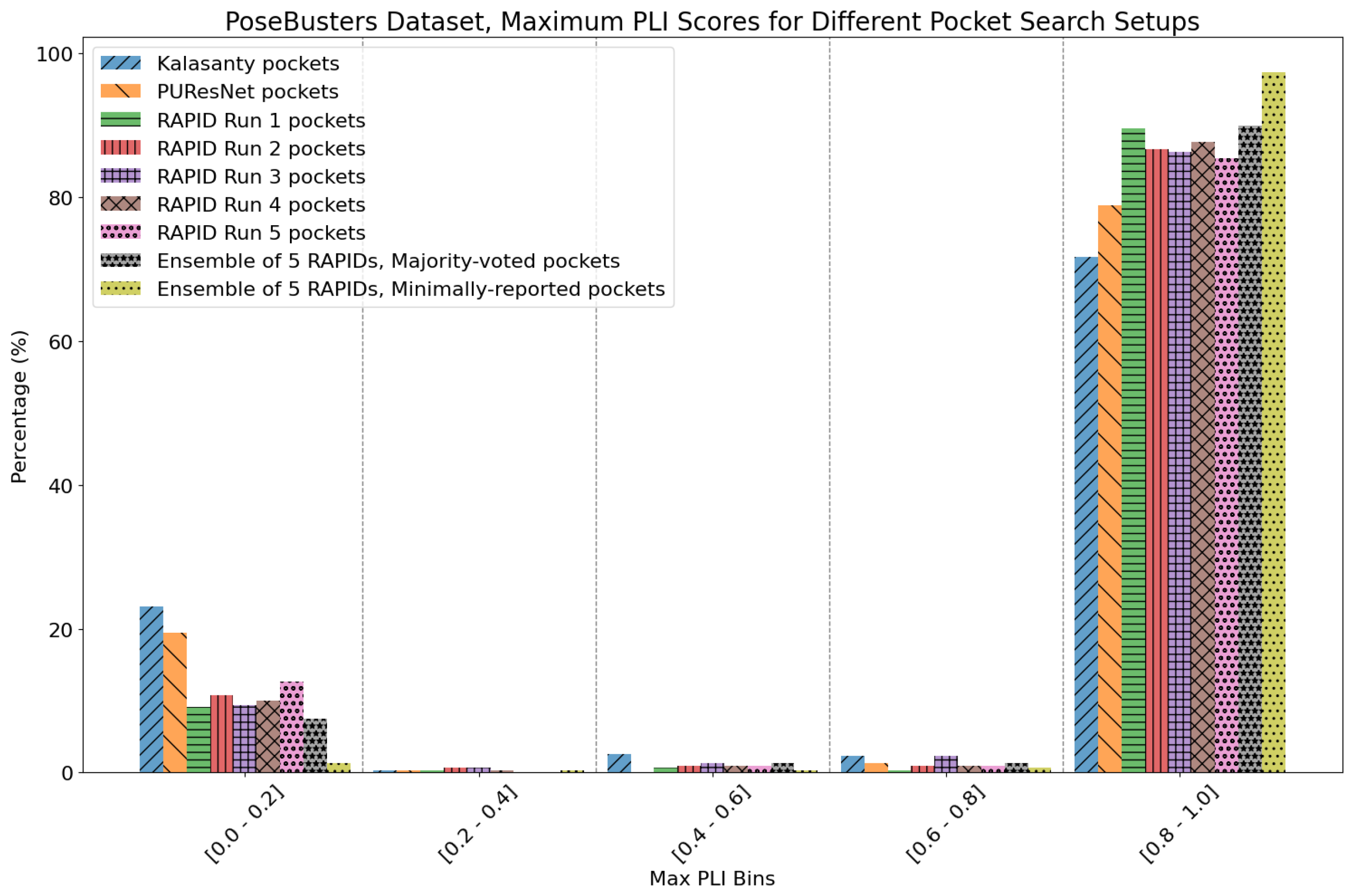
Finally, Figure 19 shows the distribution of PLI values for PUResNet [36], Kalasanty [38], and RAPID-Net for this dataset. All five replicas of RAPID-Net outperform both PUResNet [36] and Kalasanty [38]. Majority voting stabilizes the PLI predictions, and including minority-reported pockets further improves the PLI.
Figure 10.
For the 8BTI protein structure, the Top-1 Vina pose is incorrect, but the subleading pose passes all tests.
Figure 10.
For the 8BTI protein structure, the Top-1 Vina pose is incorrect, but the subleading pose passes all tests.
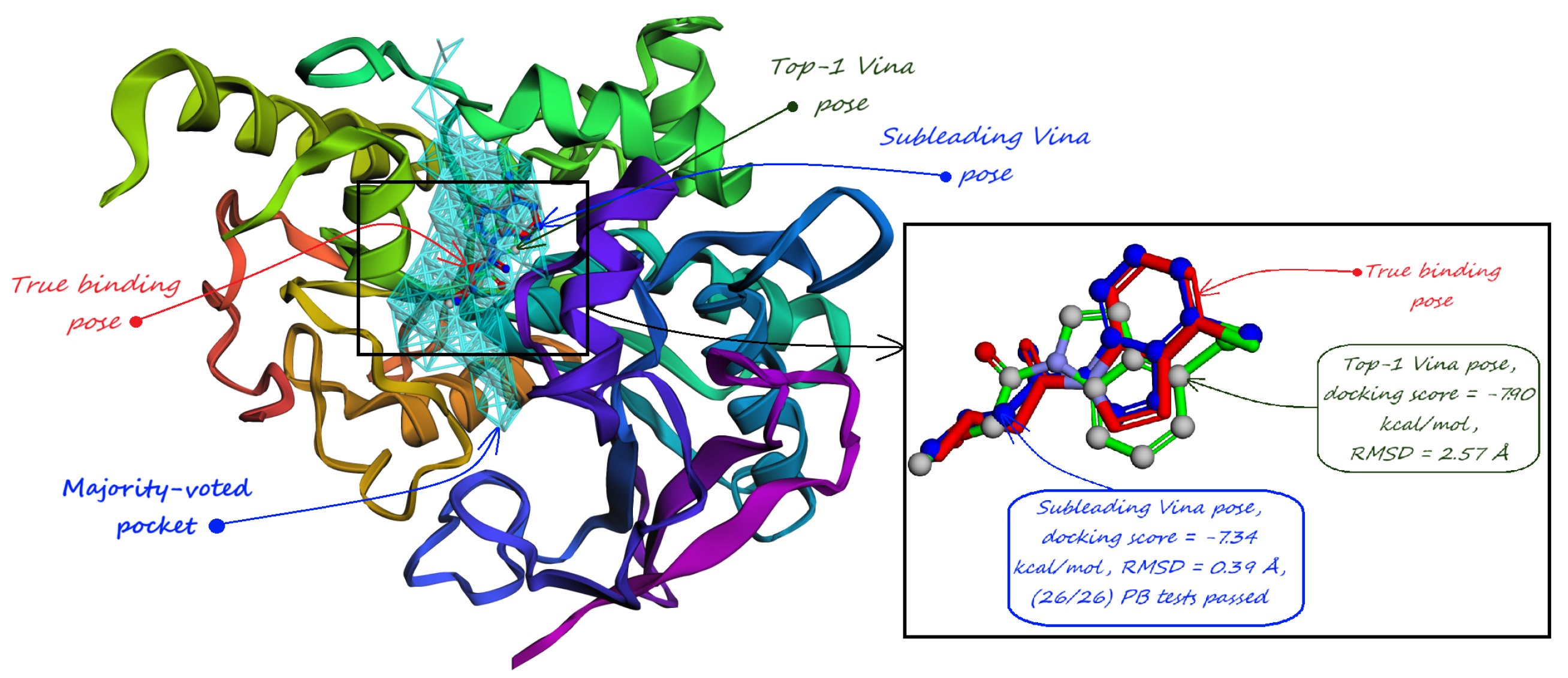
Figure 11.
For the 7XFA protein structure, neither the Top-1 nor any of the subleading Vina predicted poses pass the RMSD test, despite the predicted pocket covering the ligand with .
Figure 11.
For the 7XFA protein structure, neither the Top-1 nor any of the subleading Vina predicted poses pass the RMSD test, despite the predicted pocket covering the ligand with .
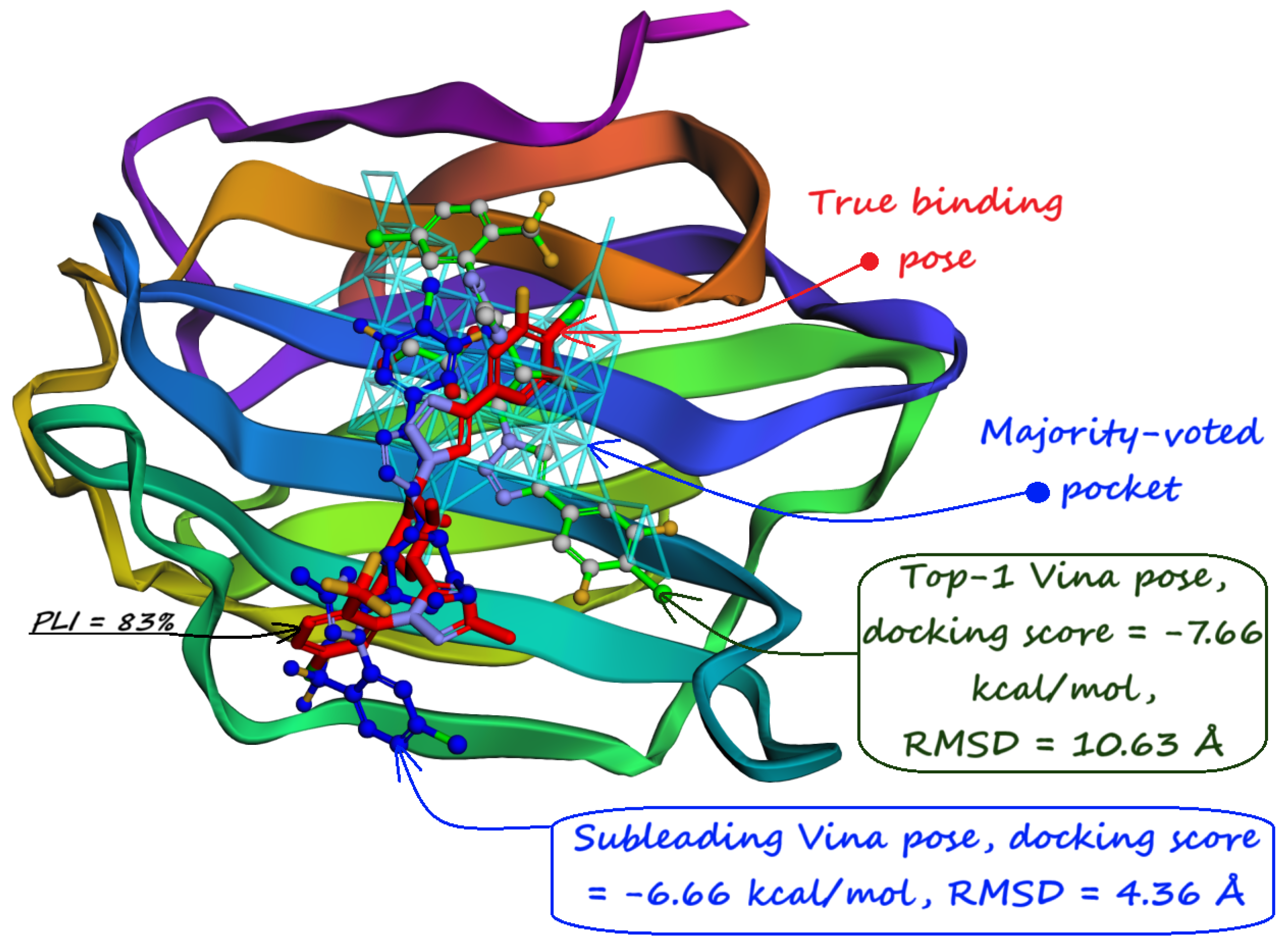
Figure 12.
Solid bars represent Top-1 accuracies. Dashed segments indicate the accuracy achievable when at least one pose in the ensemble is correct–potentially attainable with a more accurate reweighting tool.
Figure 12.
Solid bars represent Top-1 accuracies. Dashed segments indicate the accuracy achievable when at least one pose in the ensemble is correct–potentially attainable with a more accurate reweighting tool.
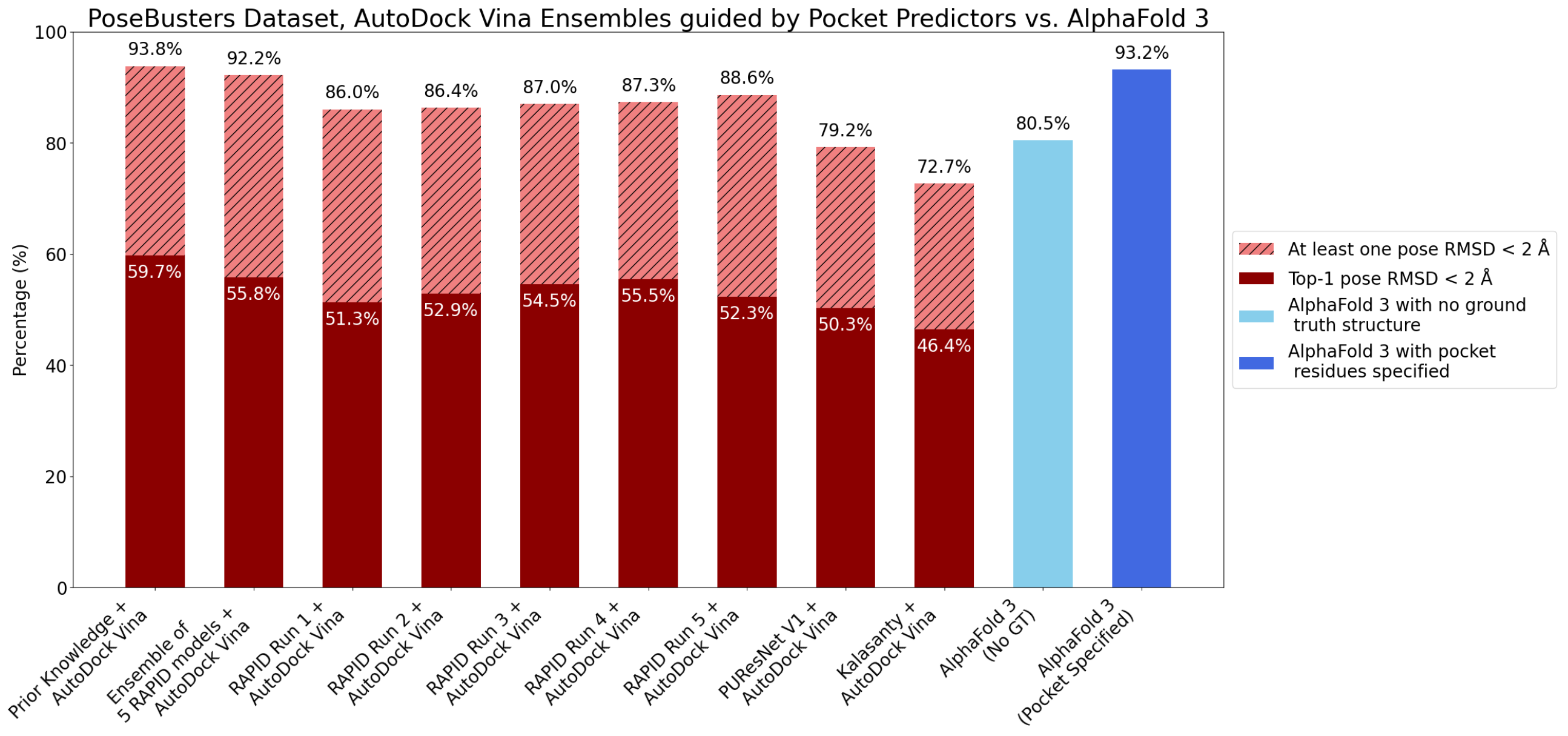
Figure 13.
Ranks of subleading Vina poses that pass the RMSD < 2 Å test when the Top-1 Vina pose fails for PoseBusters [28] dataset.
Figure 13.
Ranks of subleading Vina poses that pass the RMSD < 2 Å test when the Top-1 Vina pose fails for PoseBusters [28] dataset.
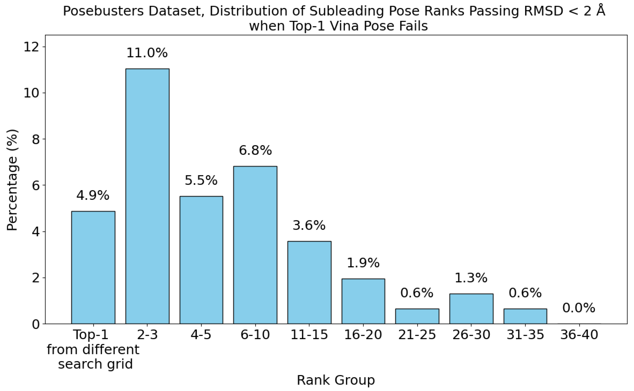
Figure 14.
For the 7PRI protein structure, the Top-1 Vina pose fails while a subleading one succeeds. In (a), the majority-voted pockets are shown in cyan, and one of the true ligand binding poses largely overlaps with one of them. In (b), minimally-reported pockets are displayed.
Figure 14.
For the 7PRI protein structure, the Top-1 Vina pose fails while a subleading one succeeds. In (a), the majority-voted pockets are shown in cyan, and one of the true ligand binding poses largely overlaps with one of them. In (b), minimally-reported pockets are displayed.
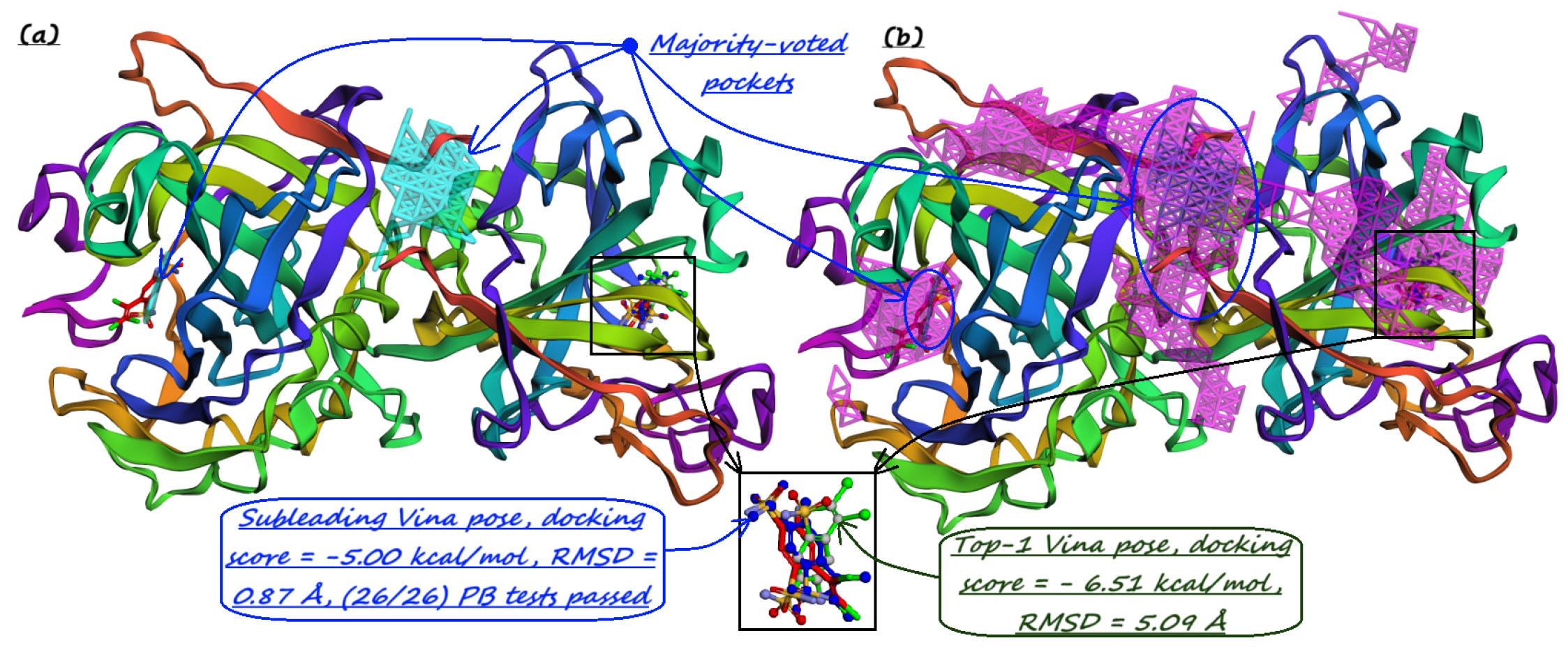
Figure 15.
In the 7P1F protein structure, two true ligand binding poses exist, both largely within the majority-voted pockets predicted by RAPID-Net. The Top-1 Vina pose is within one of these pockets but is inaccurate, failing the RMSD < 2 Å test. However, a subleading pose occupies a different pocket and passes all tests.
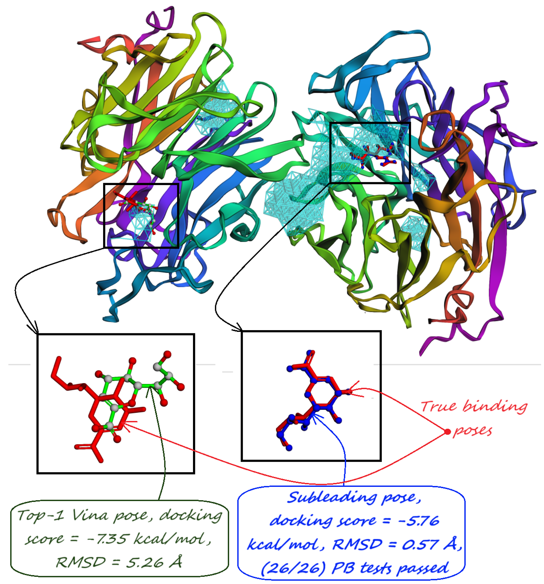
Figure 16.
For the 7NUT protein structure, there are two true ligand binding poses, both largely within majority-voted pockets predicted by RAPID-Net. The Top-1 Vina pose failing the RMSD < 2 Å test and a subleading pose passing the test are in the same majority-voted pocket.
Figure 16.
For the 7NUT protein structure, there are two true ligand binding poses, both largely within majority-voted pockets predicted by RAPID-Net. The Top-1 Vina pose failing the RMSD < 2 Å test and a subleading pose passing the test are in the same majority-voted pocket.

Figure 17.
In the 7A9E protein structure, RAPID-Net predicts a single majority-voted pocket. The Top-1 Vina pose is located in an incorrect part of that pocket, whereas a subleading pose that passes the RMSD < 2 Å test–aligning with one of the true ligand binding poses–is found in another part of the same pocket.
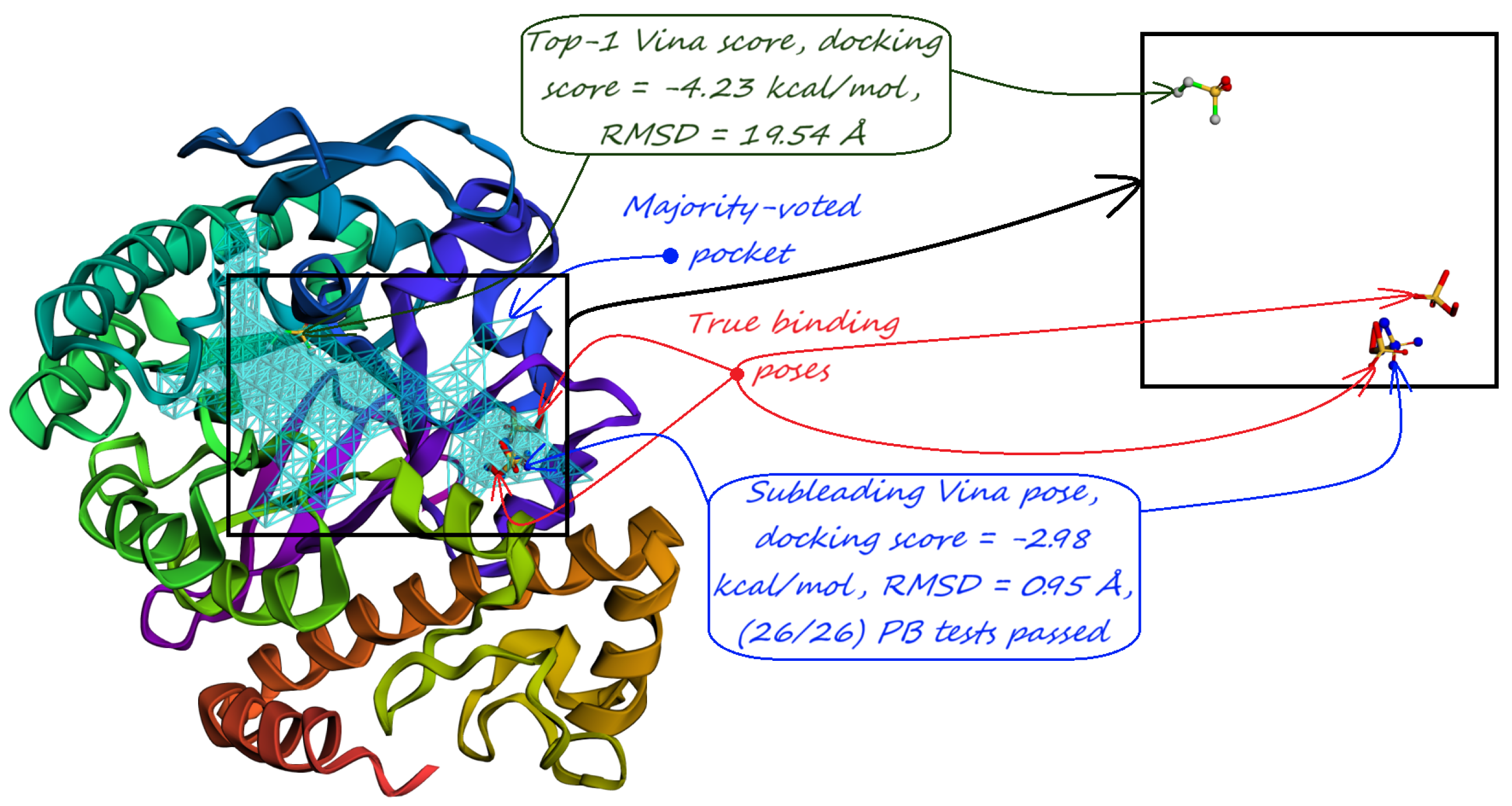
Figure 18.
Distribution of search grids leading to poses that pass the RMSD < 2 Å test, for Top-1 Vina poses and for subleading poses when the Top-1 Vina pose fails for PoseBusters [28] dataset.
Figure 18.
Distribution of search grids leading to poses that pass the RMSD < 2 Å test, for Top-1 Vina poses and for subleading poses when the Top-1 Vina pose fails for PoseBusters [28] dataset.
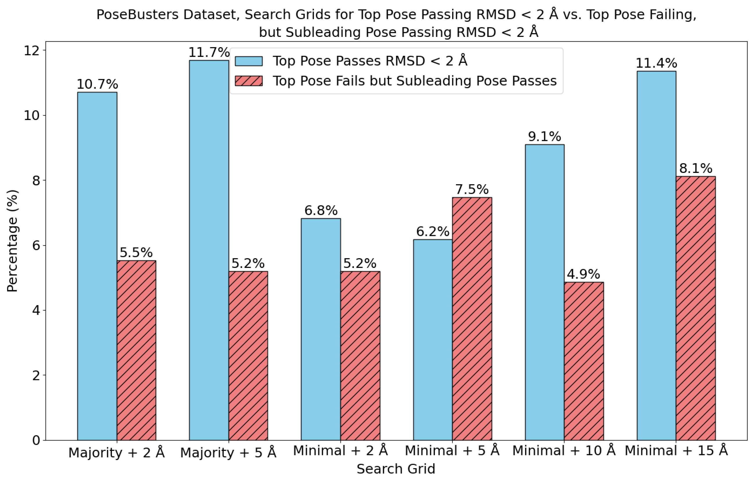
Figure 19.
Distribution of the maximum PLI scores corresponding to the pockets predicted by RAPID-Net, PUResNet [36], and Kalasanty [38] for the PoseBusters dataset [28].
To highlight the necessity of model ensembling to provide stable pocket predictions, Table 1 summarizes the level of pocket and ligand overlap and lists:
- The number of protein structures with at least one predicted pocket (shown in the “Nonzero” column). Since no protein in all our datasets is a true negative, failure to predict any pocket for a given structure is automatically an incorrect prediction.
- The number of structures with viable search grids encompassing at least one true ligand binding pose (“Within ” column), where the docking may succeed.
- The average Pocket-Ligand Intersection (PLI) value for all protein structures.
For the RAPID-Net model, individual runs show variability in pocket prediction quality. For example, Run 5 predicts pockets for all 308 protein structures but with lower accuracy, resulting in the lowest average PLI of 86.32% among the five runs. In contrast, Run 1 fails to predict pockets for one structure out of 308 but achieves the highest average PLI of 90.17% among five runs. Combining predictions via majority voting among these RAPID-Net runs increases the average PLI to 91.44%. Further incorporating minority-reported pockets boosts the average PLI even higher, to 98.09%. In the final ensemble of pockets predicted by RAPID-Net, all 308 protein structures have at least one predicted pocket and only one structure lacks a search grid covering at least one true ligand binding pose. These observations highlight the importance of combining pocket predictions from multiple runs to achieve reliable results for subsequent docking.
7. Evaluation on the Astex Diverse Set
The docking results of AutoDock Vina [12] guided by different pocket-finding algorithms for the Astex Diverse Set [29], consisting of 85 protein structures, are shown in Figure 20. The corresponding RMSD distribution of the Top-1 predicted Vina poses is presented in Figure 21, and the associated PLI scores are shown in Figure 22.
Several striking features emerge from these graphs. First, although each individual Run of our model outperforms the docking accuracy achieved when guiding AutoDock Vina [12] using PUResNet [36] or Kalasanty [38], ensembling these individual Runs does not improve the overall docking accuracy. This happens even though the ensembled version of RAPID-Net achieves a higher ligand-pocket intersection, as shown in Figure 22 and Table 2.
Furthermore, unlike the PoseBusters [28] dataset, when AutoDock Vina [12] is guided by Kalasanty [38] on the Astex Diverse Set [29], it achieves better docking accuracy than when guided by PUResNet [36], even though PUResNet [36] has more structures with at least one true ligand binding pose completely within the search grid (72 vs. 70, respectively).
Nevertheless, when considering ensemble accuracy–achieved either by the Top-1 pose or any subleading pose, as illustrated in Figure 23–the ensembled version of RAPID-Net outperforms each of its individual Runs: 95.3% versus 92.9%, 87.1%, 89.4%, 90.6%, and 91.8%, respectively. Additionally, PUResNet [36] and Kalasanty [38] both achieve the same ensemble accuracy of 78.8%. Figure 25 shows the distribution of subleading poses’ ranks passing the RMSD tests when the Top-1 Vina pose fails. For example, Figure 26 illustrates the 1G9V protein structure, where a subleading pose ranked 39 – very far from the Top-1 pose – successfully passes all validation tests, while the Top-1 Vina pose fails.
A comparison of Table 1 and Table 2 alongside Figure 12 and Figure 23 shows that RAPID-Net achieves a higher PLI rate on the Astex Diverse Set [29] than on the PoseBusters [28] dataset. However, the Top-1 docking accuracy is higher for PoseBusters [28], while the “at least one correct pose in the ensemble” accuracy is better for the Astex Diverse Set [29]. These results further emphasize and illustrate that, in addition to accurate pocket identification, another major bottleneck in the docking process is the accurate reranking of the generated poses.
In the next Section, we compare our model against other available pocket predictors in terms of PLI metrics using their original test datasets to enable a direct side-by-side comparison.
Figure 20.
Comparison of docking accuracies for the Astex Diverse Set [29] when AutoDock Vina [12] is guided by different pocket prediction algorithms.
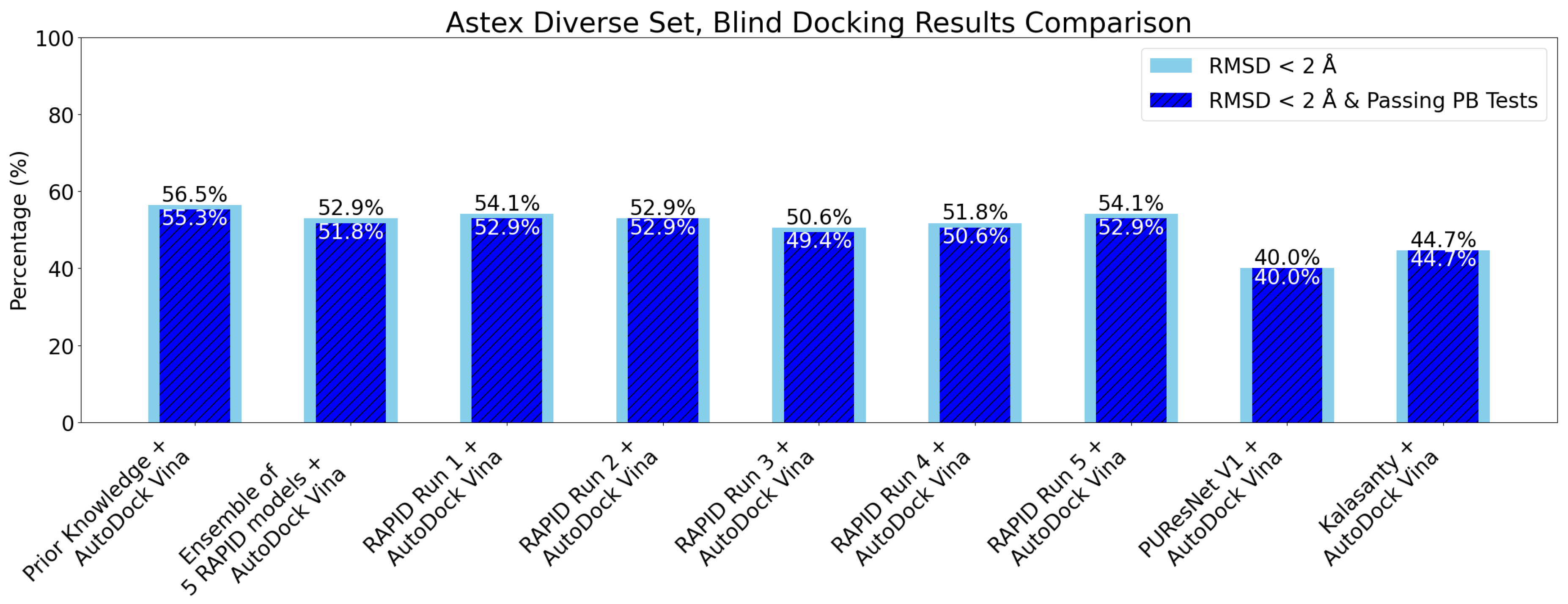
Figure 21.
Distribution of RMSD values for Top-1 Vina predicted poses in the Astex Diverse Set [28]. When multiple true ligand poses are available, the RMSD to the closest one is considered.
Figure 21.
Distribution of RMSD values for Top-1 Vina predicted poses in the Astex Diverse Set [28]. When multiple true ligand poses are available, the RMSD to the closest one is considered.
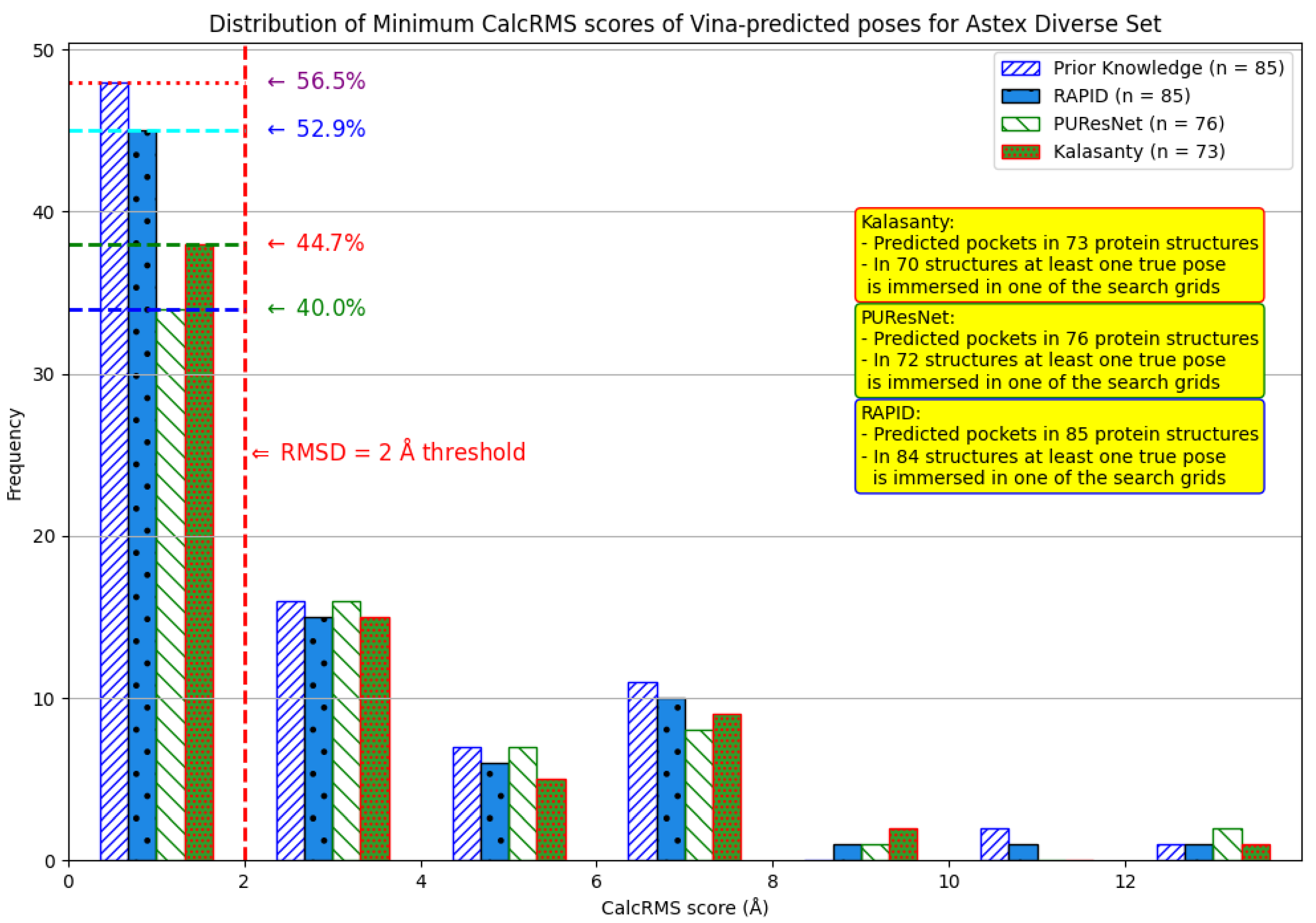
Figure 22.
Distribution of the maximum PLI scores corresponding to the pockets predicted by RAPID-Net, PUResNet [36], and Kalasanty [38] for the Astex Diverse Set [29].
Figure 23.
Docking accuracy of AutoDock Vina [12] for the Astex Diverse Set [29] when guided by different pocket prediction algorithms, comparing Top-1 and ensemble accuracy.
Figure 24.
Distribution of search grids leading to poses that pass the RMSD < 2 Å test, for Top-1 Vina poses and for subleading poses when the Top-1 Vina pose fails, for Astex Diverse Set [29].
Figure 24.
Distribution of search grids leading to poses that pass the RMSD < 2 Å test, for Top-1 Vina poses and for subleading poses when the Top-1 Vina pose fails, for Astex Diverse Set [29].
Figure 25.
Ranks of subleading Vina poses that pass the RMSD < 2 Å test when the Top-1 Vina pose fails for Astex Diverse Set [29].
Figure 25.
Ranks of subleading Vina poses that pass the RMSD < 2 Å test when the Top-1 Vina pose fails for Astex Diverse Set [29].
Figure 26.
In the 1G9V protein structure from Astex Diverse Set [29], two true ligand binding poses are observed within the same majority-voted pocket predicted by RAPID-Net. While the Top-1 Vina pose fails the RMSD test, the subleading one passes all validation tests.
Figure 26.
In the 1G9V protein structure from Astex Diverse Set [29], two true ligand binding poses are observed within the same majority-voted pocket predicted by RAPID-Net. While the Top-1 Vina pose fails the RMSD test, the subleading one passes all validation tests.
8. Evaluation on Coach420 and BU48 Datasets
For direct comparison with Kalasanty [38] and PUResNet [36], we evaluate the corresponding PLI rates on the Coach420 [30] and BU48 [31] datasets. Following [36], we exclude protein structures present in the training sets, resulting in 298 and 62 protein-ligand structures for Coach420 [30] and BU48 [31], respectively.
Unlike the original PUResNet [36] paper where PLI values were evaluated only on protein structures where the distance-center-to-center (DCC) between predicted pocket centers and ligand centers was , we report the results for all protein structures, over the whole dataset. This comparison seems more appropriate because a rough initial approximation to set up the search grid is often sufficient to achieve successful docking, as illustrated in Figure 6. Furthermore, as discussed in the next Section, the RAPID-Net model sometimes predicts meaningful “tunnels” or “bridges” to distant binding sites that indirectly influence ligand binding. In such cases, the DCC metric becomes irrelevant since it does not reflect the functional importance of these remote interactions.
Table 3 and Figure 27 summarize the results for the Coach420 dataset [30]. Except for Run 3, every RAPID-Net run surpasses PUResNet [36] and Kalasanty [38] in terms of an average PLI score. Furthermore, when comparing the number of protein structures in which at least one true ligand binding pose is entirely within the search grid, up to the largest grid with a threshold of , all RAPID-Net Runs outperform both PUResNet [36] and Kalasanty [38]. Similarly, Table 4 and Figure 28 present the results for the BU48 dataset [31]. Here, all RAPID-Net Runs, except Run 5, outperform both Kalasanty and PUResNet in terms of an average PLI and the number of protein structures where at least one true ligand binding pose is completely contained within the search grids.
Different RAPID-Net Runs have varying performances across the four test datasets, reflecting the inherent element of randomness in the model training. For example, on the PoseBusters [28] dataset, Run 2 has the fewest protein structures with viable predicted search grids, as shown in Table 1. In contrast, Run 3 produces the fewest viable grids for the Astex Diverse Set [29] and Coach420 [30], as shown in Table 2 and Table 3, while Run 5 shows the lowest PLI for BU48 [31], as shown in Table 4. Notably, despite having lower coverage on Coach420 [30] and BU48 [31], Run 5 achieves the highest “at least one correct pose in the ensemble” rate on PoseBusters [28], as shown in Figure 12.
These results further emphasize the importance of ensembling model predictions to capture all potential binding sites and account for variability in model training. By combining five RAPID-Net models, we mitigate performance defects of individual model Runs, yielding more robust and reliable results. At the same time, as can be observed from all the data that we presented, across all four test datasets, RAPID-Net consistently exhibits stronger generalization ability than both PUResNet [36] and Kalasanty [38].
In addition to docking accuracy and the coverage of true ligand binding poses by predicted pockets, it is crucial to identify relevant distant sites that indirectly influence ligand binding, which is the topic of the next Section.
9. Identification of Allosteric Sites, Exosites, and Flexible Regions for Drug Design
To illustrate RAPID-Net’s ability to identify remote sites of therapeutic interest, we consider four proteins where such sites are well documented.
Thrombin (RCSB PDB: 1DWC) The RCSB PDB entry 1DWC [65] is the crystal structure of human -thrombin in complex with the inhibitor MD-805. Thrombin plays a pivotal role in the coagulation cascade and is therefore a key target in treating acute coronary syndromes [66]. As shown in Figure 29, Kalasanty [38] and PUResNet [36] predict binding pockets largely surrounding the ligand. By contrast, our model, RAPID-Net, detects an additional bulge extending towards residues 71, 73, 75, 76, and 77. These residues belong to the anion-binding Exosite I, which interacts with negatively charged substrates and cofactors such as fibrinogen, thrombomodulin, and COOH-terminal peptide of hirudin [67,68,69,70,71]. Our model’s prediction, a “tunnel” connecting the active site to the Exosite I in Figure 29, suggests possible long-range interactions, consistent with previous studies of long-range allosteric communication in thrombin [71].
Human Carbonic Anhydrase I (RCSB PDB: 1AZM) and II (RCSB PDB: 3HS4) Human carbonic anhydrase I (hCAI) in complex with a sulfonamide drug (PDB: 1AZM) [72] and hCAII in complex with acetazolamide (AZM) (PDB: 3HS4) [73] are key targets for glaucoma treatment [74] and diuretic therapy [75], with broader potential for treating obesity, cancer, and Alzheimer’s disease [75]. In both isoforms, His64 acts as the primary proton shuttle [76,77,78].
As shown in Figure 30a, while PUResNet V1 [36] and Kalasanty [38] predict the primary ligand binding region in 1AZM, our model additionally predicts a hook-shaped bulge wrapping around His64, suggesting an allosteric interaction.
In hCAII (3HS4), a histidine cluster (His3, His4, His10, His15, His17, His64) mediates proton exchange between the active site and the environment [75]. Notably, 3HS4 contains two additional AZM molecules in shallow surface pockets–one previously identified [79,80] and another in a novel binding site [73].
As shown in Figure 30b, RAPID-Net identifies two majority-voted pockets: one around the catalytic site and another one near the histidine cluster. As shown in Figure 30c, the minority-reported pockets predicted by our model have with these secondary binding poses in shallow pockets. This highlights the ability of our model to predict all binding sites in the protein, both primary and secondary.
In comparison, for this protein structure, Kalasanty [38] predicts only the main binding site, PUResNet V1 [36] detects none, and PUResNet V2 [33] identifies only the interacting residues within the main binding site.
Ls-AChBP (RCSB PDB: 2ZJV). RCSB PDB ID 2ZJV [81] represents Lymnaea stagnalis acetylcholine-binding protein (AChBP) bound to neonicotinoid clothianidin. AChBP serves as a model for nicotinic acetylcholine receptors (nAChRs) and their allosteric transitions [82], providing insights into therapies for neurological disorders such as Alzheimer’s disease, schizophrenia, depression, attention deficit hyperactivity disorder, and tobacco addiction [83,84,85].
For the 2ZJV protein structure, neither Kalasanty [38] nor PUResNet V1 [36] predict any pockets. However, the majority-voted pockets from our model and the interacting residues of PUResNet V2 [33] illustrated in Figure 31 are predicted around all five true ligand binding positions.
Furthermore, our model’s pockets include distinct bridges toward residues Thr155-Asp160 in the flexible F-loop, suggesting indirect ligand interactions. This finding aligns with the results from [81], who highlighted that induced-fit movements of loop regions, including the F-loop, are essential for ligand recognition by neonicotinoids.
These examples demonstrate our model’s capability to identify regions influencing ligand binding–even without direct ligand contact. By revealing distal regions such as Exosite I in thrombin, His64 in hCA, and remote loop segments in Ls-AChBP, our approach provides key structural insights that can drive allosteric inhibitor design and broader therapeutic innovation.
10. Discussion and Conclusions
As the number of protein structures without known binding sites continues to grow, performing binding-site-agnostic (or “blind”) docking has become crucial for structure-guided drug design. Successful blind docking relies heavily on accurately identifying the search grid where the ligand is likely to bind. However, most existing pocket prediction tools operate irrespectively of docking pipelines and are evaluated using metrics that do not directly correlate with docking success. To address this gap, we developed RAPID-Net, an ML-based pocket identification tool specifically designed for seamless integration with docking pipelines. We tested RAPID-Net’s effectiveness in guiding blind docking using AutoDock Vina 1.2.5 [12], but our approach can be easily adapted to any docking software that requires a well-defined search grid.
When guided by RAPID-Net, AutoDock Vina [12] outperforms DiffBindFR [43] by over 5% in blind docking accuracy on the PoseBusters [28] dataset, highlighting the direct relationship between improved pocket identification and increased docking accuracy. Furthermore, RAPID-Net provides precise and compact search grids, enabling the docking of ligands to large proteins such as 8F4J from the PoseBusters [28] dataset, which tools like AlphaFold 3 [32] cannot process in whole, highlighting the critical importance of accurate and focused search areas for effective docking.
We found that another major factor limiting docking accuracy is the proper reranking of generated poses. Notably, when assessing accuracy based on whether at least one pose in the ensemble is correct (instead of only the top-ranked pose), AutoDock Vina [12] surpasses AlphaFold 3 [32] in accuracy on PoseBusters [28] dataset. This advantage becomes even more significant in blind docking scenarios. With RAPID-Net’s guidance, AutoDock Vina 1.2.5 [12] exceeds AlphaFold 3’s performance by over 10% on the PoseBusters [28] dataset. These findings suggest that, in addition to precise pocket identification, developing improved reranking tools could further enhance the docking accuracy of our combined scheme by effectively selecting the most favorable poses from those generated.
We attribute the success of RAPID-Net to the following key changes and innovations we introduced:
- Soft Labeling and ReLU Activation: Unlike conventional binary segmentation tasks, we applied soft labels and ReLU activation in the output layer, drawing inspiration from medical image segmentation techniques. This approach enables the model to more effectively differentiate between the internal regions of pockets and their boundaries.
- Attention Mechanism: We integrated a single attention block within the encoder-decoder bottleneck, enhancing the model’s ability to focus on relevant features while reducing the risk of overfit in inherently noisy data environments.
- Simplified Architecture: By eliminating excessive residual connections, we streamlined the model architecture, resulting in improved performance. This simplification was effective given the noisy nature of the dataset.
Finally, our model demonstrated the ability to identify “bridges” to distal sites located more than away from the ligand binding site, which are crucial for therapeutic applications, making RAPID-Net a promising tool for uncovering such areas and providing valuable insights for broader therapeutic strategies.
In summary, RAPID-Net not only improves the accuracy of pocket identification and subsequent docking but also opens new avenues for targeting remote therapeutic sites, highlighting its potential in the field of computational drug discovery.
Usage of Our Model and Reproducibility of Results
All code and relevant data (proteins, pockets, poses) are publicly available on GitHub 2. To reproduce our results, interested readers should download these files and follow the instructions provided in our repository.
To apply our trained model to predict pockets for other proteins and perform subsequent docking with AutoDock Vina [12], we provide an accompanying notebook with step-by-step guidance in the same repository. Additionally, our pocket predictor can be integrated with other docking tools, for example, by using spherical search grids. Users may also refine the ensemble of poses generated by AutoDock Vina [12] guided by our pocket predictor by any preferred reweighting method, leveraging our pocket predictions to improve docking accuracy.
Author Contributions
YB designed the neural network, conducted model training and docking experiments, and drafted the manuscript. IH and AB contributed to data analysis and provided medical expertise. CVK supervised the research and contributed to data analysis. All authors contributed to the proofreading and approved the final version of the manuscript.
Acknowledgments
Research reported in this publication was supported by the National Institute of Diabetes and Digestive and Kidney Diseases of the National Institutes of Health under award number R01DK076629. We are grateful to Richard J. Barber and the Barber Integrative Metabolic Research Program for financial support. We also thank James Granneman and Kelly McNear for valuable discussions.
References
- Kukol, A.; et al. Molecular modeling of proteins; Vol. 443, Springer, 2008.
- An, J.; Totrov, M.; Abagyan, R. Comprehensive identification of “druggable” protein ligand binding sites. Genome Informatics 2004, 15, 31–41. [Google Scholar] [PubMed]
- De Ruyck, J.; Brysbaert, G.; Blossey, R.; Lensink, M.F. Molecular docking as a popular tool in drug design, an in silico travel. Advances and Applications in Bioinformatics and Chemistry 2016, pp. 1–11.
- Rezaei, M.A.; Li, Y.; Wu, D.; Li, X.; Li, C. Deep learning in drug design: protein-ligand binding affinity prediction. IEEE/ACM transactions on computational biology and bioinformatics 2020, 19, 407–417. [Google Scholar] [CrossRef] [PubMed]
- Vamathevan, J.; Clark, D.; Czodrowski, P.; Dunham, I.; Ferran, E.; Lee, G.; Li, B.; Madabhushi, A.; Shah, P.; Spitzer, M.; et al. Applications of machine learning in drug discovery and development. Nature reviews Drug discovery 2019, 18, 463–477. [Google Scholar] [CrossRef]
- Saikia, S.; Bordoloi, M. Molecular docking: challenges, advances and its use in drug discovery perspective. Current drug targets 2019, 20, 501–521. [Google Scholar] [CrossRef] [PubMed]
- Zoete, V.; Grosdidier, A.; Michielin, O. Docking, virtual high throughput screening and in silico fragment-based drug design. Journal of cellular and molecular medicine 2009, 13, 238–248. [Google Scholar] [CrossRef]
- Lionta, E.; Spyrou, G.; K Vassilatis, D.; Cournia, Z. Structure-based virtual screening for drug discovery: principles, applications and recent advances. Current topics in medicinal chemistry 2014, 14, 1923–1938. [Google Scholar] [CrossRef] [PubMed]
- Patrick, G.L. An introduction to medicinal chemistry; Oxford university press, 2023.
- Hernández-Santoyo, A.; Tenorio-Barajas, A.Y.; Altuzar, V.; Vivanco-Cid, H.; Mendoza-Barrera, C. Protein-protein and protein-ligand docking. Protein engineering-technology and application 2013, pp. 63–81.
- Trott, O.; Olson, A.J. AutoDock Vina: improving the speed and accuracy of docking with a new scoring function, efficient optimization, and multithreading. Journal of computational chemistry 2010, 31, 455–461. [Google Scholar] [CrossRef]
- Eberhardt, J.; Santos-Martins, D.; Tillack, A.F.; Forli, S. AutoDock Vina 1.2. 0: New docking methods, expanded force field, and python bindings. Journal of chemical information and modeling 2021, 61, 3891–3898. [Google Scholar] [CrossRef]
- Verdonk, M.L.; Cole, J.C.; Hartshorn, M.J.; Murray, C.W.; Taylor, R.D. Improved protein–ligand docking using GOLD. Proteins: Structure, Function, and Bioinformatics 2003, 52, 609–623. [Google Scholar] [CrossRef]
- Friesner, R.A.; Banks, J.L.; Murphy, R.B.; Halgren, T.A.; Klicic, J.J.; Mainz, D.T.; Repasky, M.P.; Knoll, E.H.; Shelley, M.; Perry, J.K.; et al. Glide: a new approach for rapid, accurate docking and scoring. 1. Method and assessment of docking accuracy. Journal of medicinal chemistry 2004, 47, 1739–1749. [Google Scholar] [CrossRef]
- Grasso, G.; Di Gregorio, A.; Mavkov, B.; Piga, D.; Labate, G.F.D.; Danani, A.; Deriu, M.A. Fragmented blind docking: a novel protein–ligand binding prediction protocol. Journal of Biomolecular Structure and Dynamics 2022, 40, 13472–13481. [Google Scholar] [CrossRef]
- Hassan, N.M.; Alhossary, A.A.; Mu, Y.; Kwoh, C.K. Protein-ligand blind docking using QuickVina-W with inter-process spatio-temporal integration. Scientific reports 2017, 7, 15451. [Google Scholar] [CrossRef] [PubMed]
- Koes, D.R.; Baumgartner, M.P.; Camacho, C.J. Lessons learned in empirical scoring with smina from the CSAR 2011 benchmarking exercise. Journal of chemical information and modeling 2013, 53, 1893–1904. [Google Scholar] [CrossRef] [PubMed]
- Shen, Y. Predicting protein structure from single sequences. Nature Computational Science 2022, 2, 775–776. [Google Scholar] [CrossRef] [PubMed]
- Jumper, J.; Evans, R.; Pritzel, A.; Green, T.; Figurnov, M.; Ronneberger, O.; Tunyasuvunakool, K.; Bates, R.; Žídek, A.; Potapenko, A.; et al. Highly accurate protein structure prediction with AlphaFold. nature 2021, 596, 583–589. [Google Scholar] [CrossRef]
- Mirdita, M.; Schütze, K.; Moriwaki, Y.; Heo, L.; Ovchinnikov, S.; Steinegger, M. ColabFold: making protein folding accessible to all. Nature methods 2022, 19, 679–682. [Google Scholar] [CrossRef]
- Ahdritz, G.; Bouatta, N.; Floristean, C.; Kadyan, S.; Xia, Q.; Gerecke, W.; O’Donnell, T.J.; Berenberg, D.; Fisk, I.; Zanichelli, N.; et al. OpenFold: Retraining AlphaFold2 yields new insights into its learning mechanisms and capacity for generalization. Nature Methods 2024, pp. 1–11.
- Baek, M.; DiMaio, F.; Anishchenko, I.; Dauparas, J.; Ovchinnikov, S.; Lee, G.R.; Wang, J.; Cong, Q.; Kinch, L.N.; Schaeffer, R.D.; et al. Accurate prediction of protein structures and interactions using a three-track neural network. Science 2021, 373, 871–876. [Google Scholar] [CrossRef]
- Overington, J.P.; Al-Lazikani, B.; Hopkins, A.L. How many drug targets are there? Nature reviews Drug discovery 2006, 5, 993–996. [Google Scholar] [CrossRef]
- Santos, R.; Ursu, O.; Gaulton, A.; Bento, A.P.; Donadi, R.S.; Bologa, C.G.; Karlsson, A.; Al-Lazikani, B.; Hersey, A.; Oprea, T.I.; et al. A comprehensive map of molecular drug targets. Nature reviews Drug discovery 2017, 16, 19–34. [Google Scholar] [CrossRef]
- Huang, Y.; Zhang, H.; Jiang, S.; Yue, D.; Lin, X.; Zhang, J.; Gao, Y.Q. DSDP: a blind docking strategy accelerated by GPUs. Journal of Chemical Information and Modeling 2023, 63, 4355–4363. [Google Scholar] [CrossRef]
- Utgés, J.S.; Barton, G.J. Comparative evaluation of methods for the prediction of protein–ligand binding sites. Journal of Cheminformatics 2024, 16, 126. [Google Scholar] [CrossRef] [PubMed]
- Chollet, F. Deep learning with Python; Simon and Schuster, 2021.
- Buttenschoen, M.; Morris, G.M.; Deane, C.M. PoseBusters: AI-based docking methods fail to generate physically valid poses or generalise to novel sequences. Chemical Science 2024, 15, 3130–3139. [Google Scholar] [CrossRef] [PubMed]
- Hartshorn, M.J.; Verdonk, M.L.; Chessari, G.; Brewerton, S.C.; Mooij, W.T.; Mortenson, P.N.; Murray, C.W. Diverse, high-quality test set for the validation of protein- ligand docking performance. Journal of Medicinal Chemistry 2007, 50, 726–741. [Google Scholar] [CrossRef] [PubMed]
- Roy, A.; Yang, J.; Zhang, Y. COFACTOR: an accurate comparative algorithm for structure-based protein function annotation. Nucleic Acids Research 2012, 40, W471–W477. [Google Scholar] [CrossRef]
- Huang, B.; Schroeder, M. LIGSITE csc: predicting ligand binding sites using the Connolly surface and degree of conservation. BMC Structural Biology 2006, 6, 1–11. [Google Scholar] [CrossRef]
- Abramson, J.; Adler, J.; Dunger, J.; Evans, R.; Green, T.; Pritzel, A.; Jumper, J.M. Accurate structure prediction of biomolecular interactions with AlphaFold 3. Nature 2024, pp. 1–3.
- Jeevan, K.; Palistha, S.; Tayara, H.; Chong, K.T. PUResNetV2.0: a deep learning model leveraging sparse representation for improved ligand binding site prediction. Journal of Cheminformatics 2024, 16, 1–16. [Google Scholar] [CrossRef]
- Sestak, F.; Schneckenreiter, L.; Brandstetter, J.; Hochreiter, S.; Mayr, A.; Klambauer, G. VN-EGNN: E (3)-Equivariant Graph Neural Networks with Virtual Nodes Enhance Protein Binding Site Identification. arXiv preprint arXiv:2404.07194 2024.
- Smith, Z.; Strobel, M.; Vani, B.P.; Tiwary, P. Graph attention site prediction (grasp): Identifying druggable binding sites using graph neural networks with attention. Journal of chemical information and modeling 2024, 64, 2637–2644. [Google Scholar] [CrossRef]
- Kandel, J.; Tayara, H.; Chong, K.T. PUResNet: prediction of protein-ligand binding sites using deep residual neural network. Journal of cheminformatics 2021, 13, 1–14. [Google Scholar] [CrossRef]
- Le Guilloux, V.; Schmidtke, P.; Tuffery, P. Fpocket: an open source platform for ligand pocket detection. BMC bioinformatics 2009, 10, 1–11. [Google Scholar] [CrossRef]
- Stepniewska-Dziubinska, M.M.; Zielenkiewicz, P.; Siedlecki, P. Improving detection of protein-ligand binding sites with 3D segmentation. Scientific Reports 2020, 10, 5035. [Google Scholar] [CrossRef]
- Krivák, R.; Hoksza, D. Improving protein-ligand binding site prediction accuracy by classification of inner pocket points using local features. Journal of cheminformatics 2015, 7, 1–13. [Google Scholar] [CrossRef] [PubMed]
- Aggarwal, R.; Gupta, A.; Chelur, V.; Jawahar, C.; Priyakumar, U.D. DeepPocket: ligand binding site detection and segmentation using 3D convolutional neural networks. Journal of Chemical Information and Modeling 2021, 62, 5069–5079. [Google Scholar] [CrossRef] [PubMed]
- Carbery, A.; Buttenschoen, M.; Skyner, R.; von Delft, F.; Deane, C.M. Learnt representations of proteins can be used for accurate prediction of small molecule binding sites on experimentally determined and predicted protein structures. Journal of Cheminformatics 2024, 16, 32. [Google Scholar] [CrossRef] [PubMed]
- Shen, A.; Yuan, M.; Ma, Y.; Du, J.; Wang, M. PGBind: pocket-guided explicit attention learning for protein–ligand docking. Briefings in Bioinformatics 2024, 25, bbae455. [Google Scholar] [CrossRef]
- Zhu, J.; Gu, Z.; Pei, J.; Lai, L. DiffBindFR: an SE(3) equivariant network for flexible protein-ligand docking. Chemical Science 2024, 15, 7926–7942, Supplementaryinformationavailable:PDF(1982K),. [Google Scholar] [CrossRef]
- Ronneberger, O.; Fischer, P.; Brox, T. U-Net: Convolutional networks for biomedical image segmentation. arXiv preprint arXiv:1505.04597 2015.
- He, K.; Zhang, X.; Ren, S.; Sun, J. Deep residual learning for image recognition. In Proceedings of the Proceedings of the IEEE conference on computer vision and pattern recognition, 2016, pp. 770–778.
- Hu, J.; Shen, L.; Sun, G. Squeeze-and-excitation networks. In Proceedings of the Proceedings of the IEEE conference on computer vision and pattern recognition, 2018, pp. 7132–7141.
- Jiang, Y.; Chen, L.; Zhang, H.; Xiao, X. Breast cancer histopathological image classification using convolutional neural networks with small SE-ResNet module. PloS One 2019, 14, e0214587. [Google Scholar] [CrossRef]
- Balytskyi, Y.; Kalashnyk, N.; Hubenko, I.; Balytska, A.; McNear, K. Enhancing Open-World Bacterial Raman Spectra Identification by Feature Regularization for Improved Resilience against Unknown Classes. Chemical & Biomedical Imaging 2024, 2, 442–452. [Google Scholar]
- Desaphy, J.; Bret, G.; Rognan, D.; Kellenberger, E. sc-PDB: a 3D-database of ligandable binding sites—10 years on. Nucleic Acids Research 2015, 43, D399–D404. [Google Scholar] [CrossRef]
- Desaphy, J.; Azdimousa, K.; Kellenberger, E.; Rognan, D. Comparison and druggability prediction of protein–ligand binding sites from pharmacophore-annotated cavity shapes. Journal of Chemical Information and Modeling 2012, 52, 2287–2299. [Google Scholar] [CrossRef]
- Kellenberger, E.; Schalon, C.; Rognan, D. How to measure the similarity between protein ligand-binding sites? Current Computer-Aided Drug Design 2008, 4, 209. [Google Scholar] [CrossRef]
- Bajusz, D.; Rácz, A.; Héberger, K. Why is Tanimoto index an appropriate choice for fingerprint-based similarity calculations? Journal of Cheminformatics 2015, 7, 1–13. [Google Scholar] [CrossRef] [PubMed]
- García-García, J.; Others. tfbio: Molecular features featurization library for TensorFlow. https://github.com/gnina/tfbio, 2018. Accessed: YYYY-MM-DD.
- Gros, C.; Lemay, A.; Cohen-Adad, J. SoftSeg: Advantages of soft versus binary training for image segmentation. Medical Image Analysis 2021, 71, 102038. [Google Scholar] [CrossRef] [PubMed]
- Wang, Z.; Popordanoska, T.; Bertels, J.; Lemmens, R.; Blaschko, M.B. Dice semimetric losses: Optimizing the dice score with soft labels. In Proceedings of the International Conference on Medical Image Computing and Computer-Assisted Intervention, Cham, 2023; pp. 475–485.
- Milletari, F.; Navab, N.; Ahmadi, S.A. V-net: Fully convolutional neural networks for volumetric medical image segmentation. In Proceedings of the 2016 Fourth International Conference on 3D Vision (3DV). IEEE, 2016, pp. 565–571.
- Lin, T.Y.; Goyal, P.; Girshick, R.; He, K.; Dollár, P. Focal Loss for Dense Object Detection. In Proceedings of the Proceedings of the IEEE International Conference on Computer Vision (ICCV), October 2017, pp. 2980–2988.
- Nair, V.; Hinton, G.E. Rectified Linear Units Improve Restricted Boltzmann Machines. In Proceedings of the Proceedings of the 27th International Conference on Machine Learning (ICML), 2010, pp. 807–814.
- Pedregosa, F.; Varoquaux, G.; Gramfort, A.; Michel, V.; Thirion, B.; Grisel, O.; Blondel, M.; Prettenhofer, P.; Weiss, R.; Dubourg, V.; et al. Scikit-learn: Machine Learning in Python. Journal of Machine Learning Research 2011, 12, 2825–2830. [Google Scholar]
- Virtanen, P.; Gommers, R.; Oliphant, T.E.; Haberland, M.; Reddy, T.; Cournapeau, D.; Burovski, E.; Peterson, P.; Weckesser, W.; Bright, J.; et al. SciPy 1.0: Fundamental Algorithms for Scientific Computing in Python. Nature Methods 2020, 17, 261–272. [Google Scholar] [CrossRef] [PubMed]
- Landrum, G. Rdkit documentation. Release 2013, 1, 4. [Google Scholar]
- Su, M.; Yang, Q.; Du, Y.; Feng, G.; Liu, Z.; Li, Y.; Wang, R. Comparative assessment of scoring functions: the CASF-2016 update. Journal of chemical information and modeling 2018, 59, 895–913. [Google Scholar] [CrossRef] [PubMed]
- Li, H.; Han, L.; Liu, W.; Wang, R. DELPHI Scorer: A Machine-Learning-Based Scoring Function for Protein-Ligand Interactions. Journal of Chemical Information and Modeling 2017, 57, 47–55. [Google Scholar] [CrossRef]
- Shen, C.; Zhang, X.; Deng, Y.; Gao, J.; Wang, D.; Xu, L.; Kang, Y. Boosting protein–ligand binding pose prediction and virtual screening based on residue–atom distance likelihood potential and graph transformer. Journal of Medicinal Chemistry 2022, 65, 10691–10706. [Google Scholar] [CrossRef]
- Banner, D.W.; Hadváry, P. Crystallographic analysis at 3.0-A resolution of the binding to human thrombin of four active site-directed inhibitors. Journal of Biological Chemistry 1991, 266, 20085–20093. [Google Scholar] [CrossRef]
- Weitz, J.I.; Buller, H.R. Direct thrombin inhibitors in acute coronary syndromes: present and future. Circulation 2002, 105, 1004–1011. [Google Scholar] [CrossRef]
- Crawley, J.T.B.; Zanardelli, S.; Chion, C.K.N.K.; Lane, D.A. The central role of thrombin in hemostasis. Journal of Thrombosis and Haemostasis 2007, 5, 95–101. [Google Scholar] [CrossRef]
- Adams, T.E.; Huntington, J.A. Thrombin-cofactor interactions: structural insights into regulatory mechanisms. Arteriosclerosis, thrombosis, and vascular biology 2006, 26, 1738–1745. [Google Scholar] [CrossRef] [PubMed]
- Bock, P.; Panizzi, P.; Verhamme, I. Exosites in the substrate specificity of blood coagulation reactions. Journal of Thrombosis and Haemostasis 2007, 5, 81–94. [Google Scholar] [CrossRef] [PubMed]
- Troisi, R.; Balasco, N.; Autiero, I.; Vitagliano, L.; Sica, F. Exosite binding in thrombin: a global structural/dynamic overview of complexes with aptamers and other ligands. International Journal of Molecular Sciences 2021, 22, 10803. [Google Scholar] [CrossRef] [PubMed]
- Petrera, N.S.; Stafford, A.R.; Leslie, B.A.; Kretz, C.A.; Fredenburgh, J.C.; Weitz, J.I. Long range communication between exosites 1 and 2 modulates thrombin function. Journal of Biological Chemistry 2009, 284, 25620–25629. [Google Scholar] [CrossRef] [PubMed]
- Chakravarty, S.; Kannan, K. Drug-protein interactions: refined structures of three sulfonamide drug complexes of human carbonic anhydrase I enzyme. Journal of molecular biology 1994, 243, 298–309. [Google Scholar] [CrossRef]
- Sippel, K.H.; Robbins, A.H.; Domsic, J.; Genis, C.; Agbandje-McKenna, M.; McKenna, R. High-resolution structure of human carbonic anhydrase II complexed with acetazolamide reveals insights into inhibitor drug design. Acta Crystallographica Section F: Structural Biology and Crystallization Communications 2009, 65, 992–995. [Google Scholar] [CrossRef]
- Pfeiffer, N. Innovative glaucoma therapy: Glaucoma therapy with topical carbonic anhydrase inhibitors. Der Ophthalmologe: Zeitschrift der Deutschen Ophthalmologischen Gesellschaft 2001, 98, 953–960. [Google Scholar] [CrossRef]
- Supuran, C.T. Carbonic anhydrases: Novel therapeutic applications for inhibitors and activators. Nature Reviews Drug Discovery 2008, 7, 168–181. [Google Scholar] [CrossRef]
- Silverman, D.N.; Lindskog, S. The catalytic mechanism of carbonic anhydrase: implications of a rate-limiting protolysis of water. Accounts of Chemical Research 1988, 21, 30–36. [Google Scholar] [CrossRef]
- Nair, S.K.; Christianson, D.W. Unexpected pH-dependent conformation of His-64, the proton shuttle of carbonic anhydrase II. Journal of the American Chemical Society 1991, 113, 9455–9458. [Google Scholar] [CrossRef]
- Lomelino, C.L.; Andring, J.T.; McKenna, R. Crystallography and its impact on carbonic anhydrase research. International journal of medicinal chemistry 2018, 2018, 9419521. [Google Scholar] [CrossRef] [PubMed]
- Jude, K.M.; Banerjee, A.L.; Haldar, M.K.; Manokaran, S.; Roy, B.; Mallik, S.; Srivastava, D.; Christianson, D.W. Ultrahigh resolution crystal structures of human carbonic anhydrases I and II complexed with “two-prong” inhibitors reveal the molecular basis of high affinity. Journal of the American Chemical Society 2006, 128, 3011–3018. [Google Scholar] [CrossRef]
- Srivastava, D.; Jude, K.M.; Banerjee, A.L.; Haldar, M.; Manokaran, S.; Kooren, J.; Mallik, S.; Christianson, D.W. Structural analysis of charge discrimination in the binding of inhibitors to human carbonic anhydrases I and II. Journal of the American Chemical Society 2007, 129, 5528–5537. [Google Scholar] [CrossRef] [PubMed]
- Ihara, M.; Okajima, T.; Yamashita, A.; Oda, T.; Hirata, K.; Nishiwaki, H.; Morimoto, T.; Akamatsu, M.; Ashikawa, Y.; Kuroda, S.; et al. Crystal structures of Lymnaea stagnalis AChBP in complex with neonicotinoid insecticides imidacloprid and clothianidin. Invertebrate Neuroscience 2008, 8, 71–81. [Google Scholar] [CrossRef] [PubMed]
- Taly, A.; Corringer, P.J.; Guedin, D.; Lestage, P.; Changeux, J.P. Nicotinic receptors: allosteric transitions and therapeutic targets in the nervous system. Nature reviews Drug discovery 2009, 8, 733–750. [Google Scholar] [CrossRef]
- Arneric, S.P.; Holladay, M.; Williams, M. Neuronal nicotinic receptors: a perspective on two decades of drug discovery research. Biochemical pharmacology 2007, 74, 1092–1101. [Google Scholar] [CrossRef] [PubMed]
- Levin, E.D.; Rezvani, A.H. Nicotinic interactions with antipsychotic drugs, models of schizophrenia and impacts on cognitive function. Biochemical Pharmacology 2007, 74, 1182–1191. [Google Scholar] [CrossRef]
- Romanelli, M.N.; Gratteri, P.; Guandalini, L.; Martini, E.; Bonaccini, C.; Gualtieri, F. Central nicotinic receptors: structure, function, ligands, and therapeutic potential. ChemMedChem: Chemistry Enabling Drug Discovery 2007, 2, 746–767. [Google Scholar] [CrossRef]
| 1 | PUResNet V1[36] predicts cavities where the ligand is likely to reside, whereas PUResNet V2 [33] predicts residues likely to interact with the ligand. For simplicity, we refer to PUResNet V1 as “PUResNet” throughout the text, as in this work we focus on cavities for generating an accurate search grid for subsequent docking. |
| 2 |
Figure 6.
For the 8FAV protein structure, our model predictions are inaccurate, and none of the true ligand binding poses are within one of the predicted pockets. Nevertheless, the docking is successful because the search grids with large thresholds smooths out this drawback.
Figure 6.
For the 8FAV protein structure, our model predictions are inaccurate, and none of the true ligand binding poses are within one of the predicted pockets. Nevertheless, the docking is successful because the search grids with large thresholds smooths out this drawback.
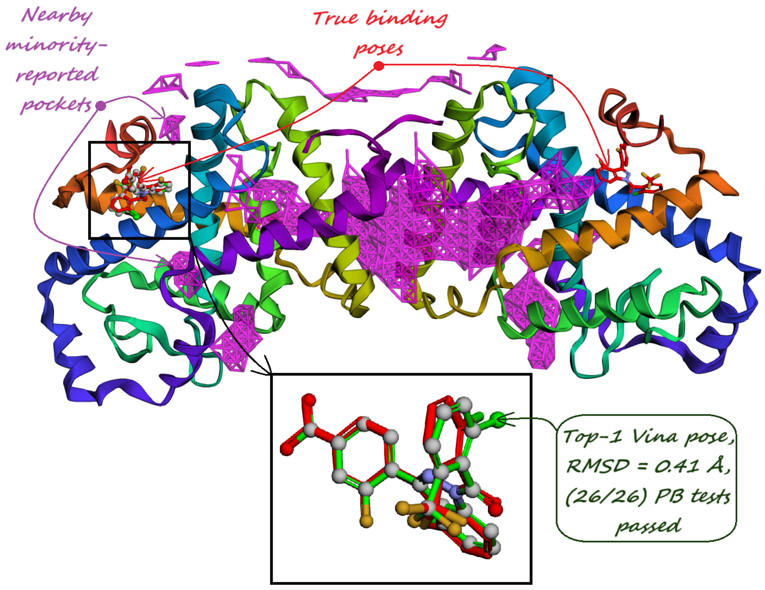
Figure 7.
Comparison of Top-1 Vina accuracies when guided by different pocket identification algorithms, and a DiffBindFR-Smina [43], for PoseBusters [28] dataset.

Figure 8.
Distribution of RMSD values for Top-1 Vina predicted poses in the PoseBusters [28] dataset. When multiple true ligand poses are available, RMSD to the closest one is reported.
Figure 8.
Distribution of RMSD values for Top-1 Vina predicted poses in the PoseBusters [28] dataset. When multiple true ligand poses are available, RMSD to the closest one is reported.
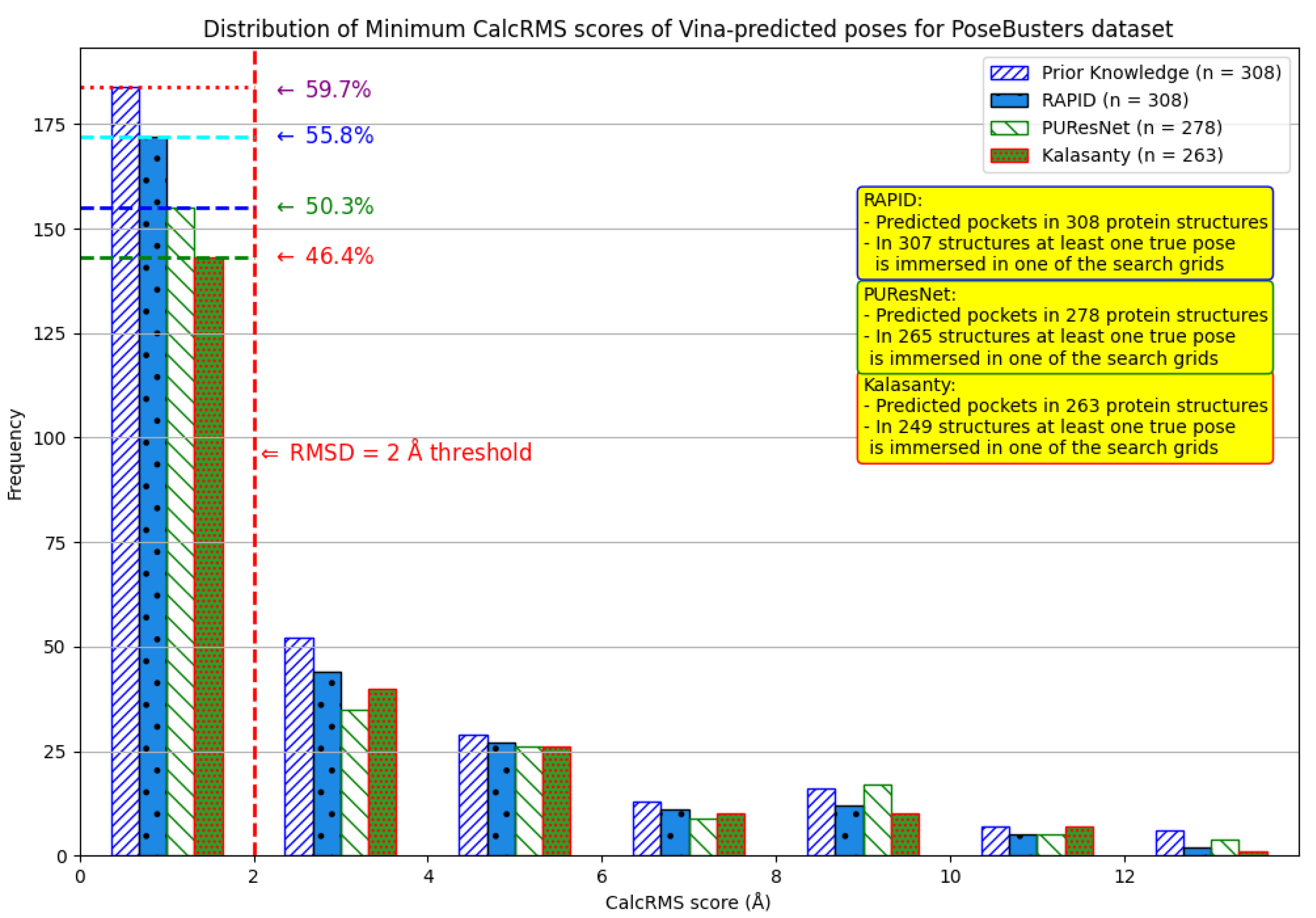
Figure 9.
In 7KZ9 protein structure, RAPID-Net predicts majority-voted pockets around both true binding poses, and the Top-1 Vina pose passes all tests.
Figure 9.
In 7KZ9 protein structure, RAPID-Net predicts majority-voted pockets around both true binding poses, and the Top-1 Vina pose passes all tests.
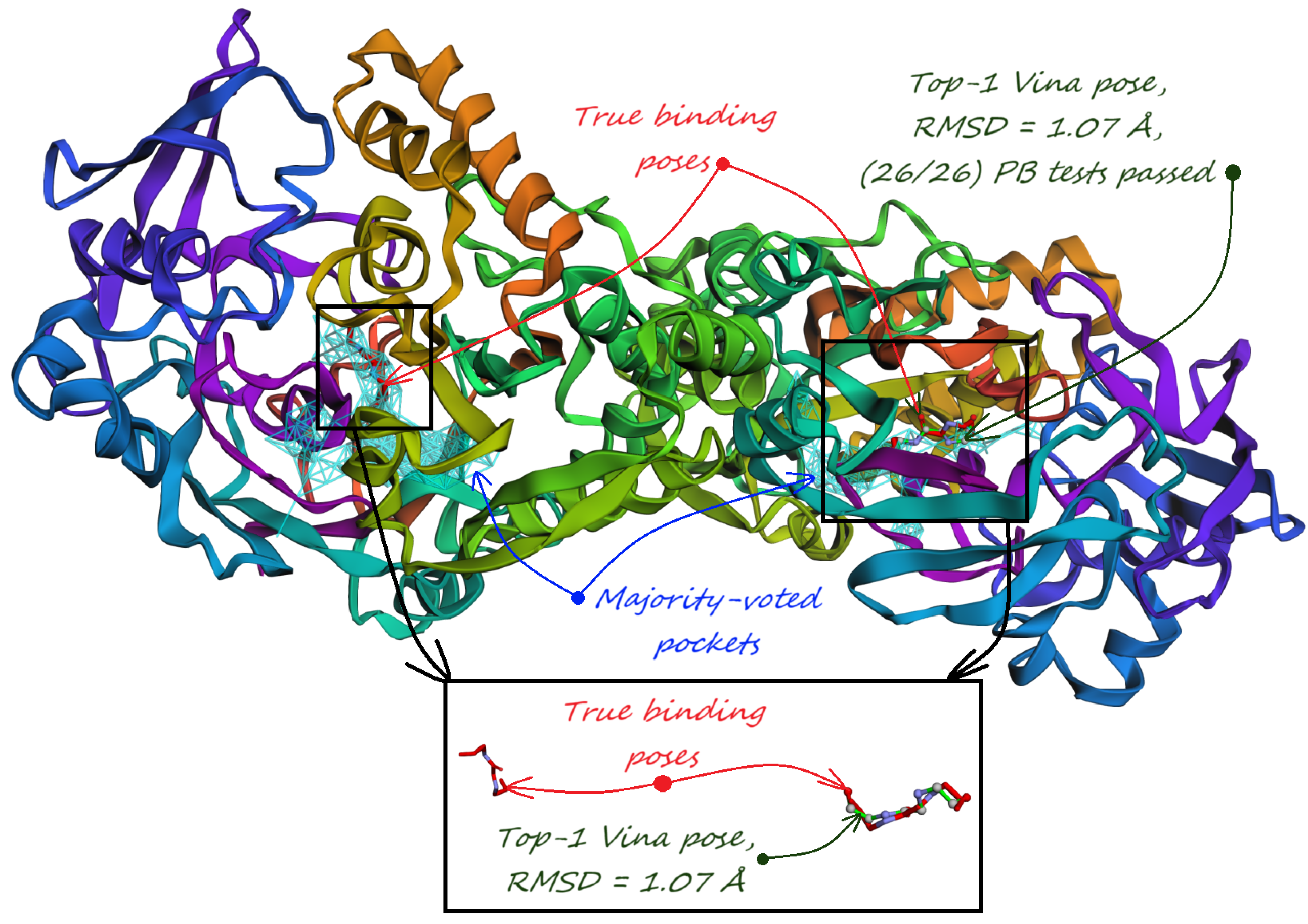
Figure 27.
Distribution of the maximum PLI scores corresponding to the pockets predicted by RAPID-Net, PUResNet [36], and Kalasanty [38] for the Coach420 [30] dataset.
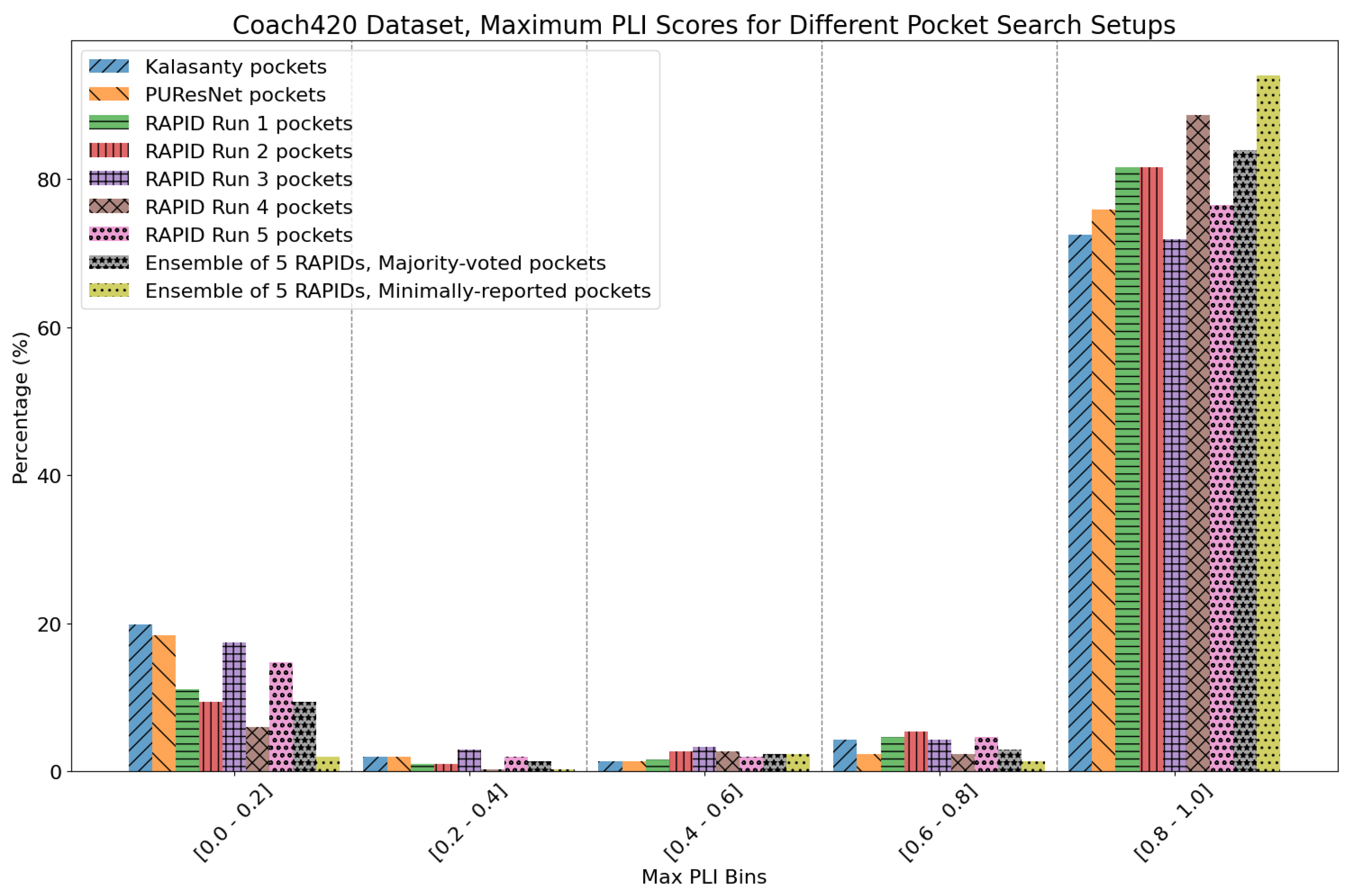
Figure 28.
Distribution of the maximum PLI scores corresponding to the pockets predicted by RAPID-Net, PUResNet [36], and Kalasanty [38] for the BU48 [31] dataset.
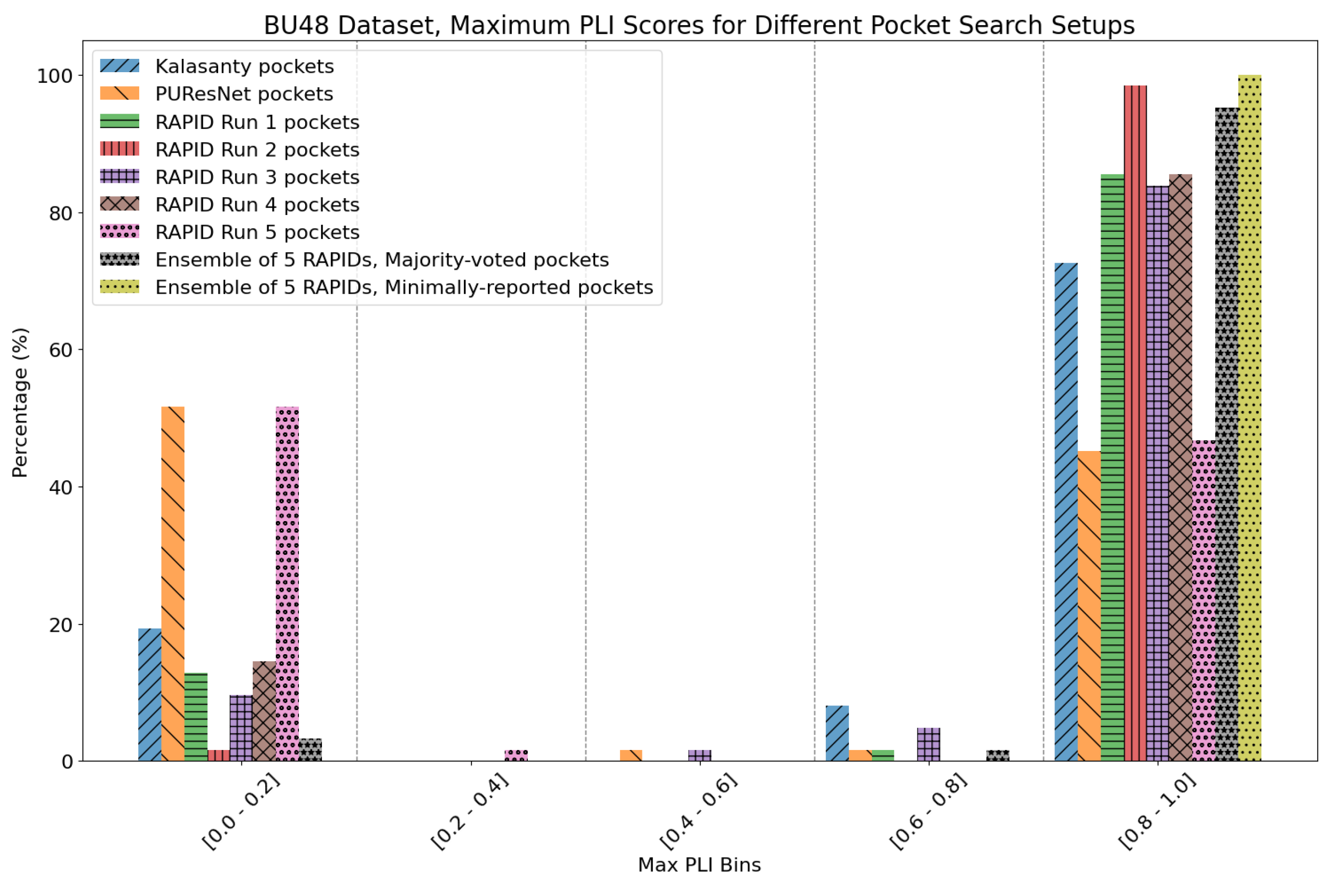
Figure 29.
Thrombin (RCSB PDB: 1DWC). Pockets predicted by Kalasanty [38] and PUResNet [36] are shown as green and orange dots respectively. The majority-voted pocket predicted by our model is shown as cyan sticks where one can observe a distinct bulge towards the residues belonging to Exosite I.
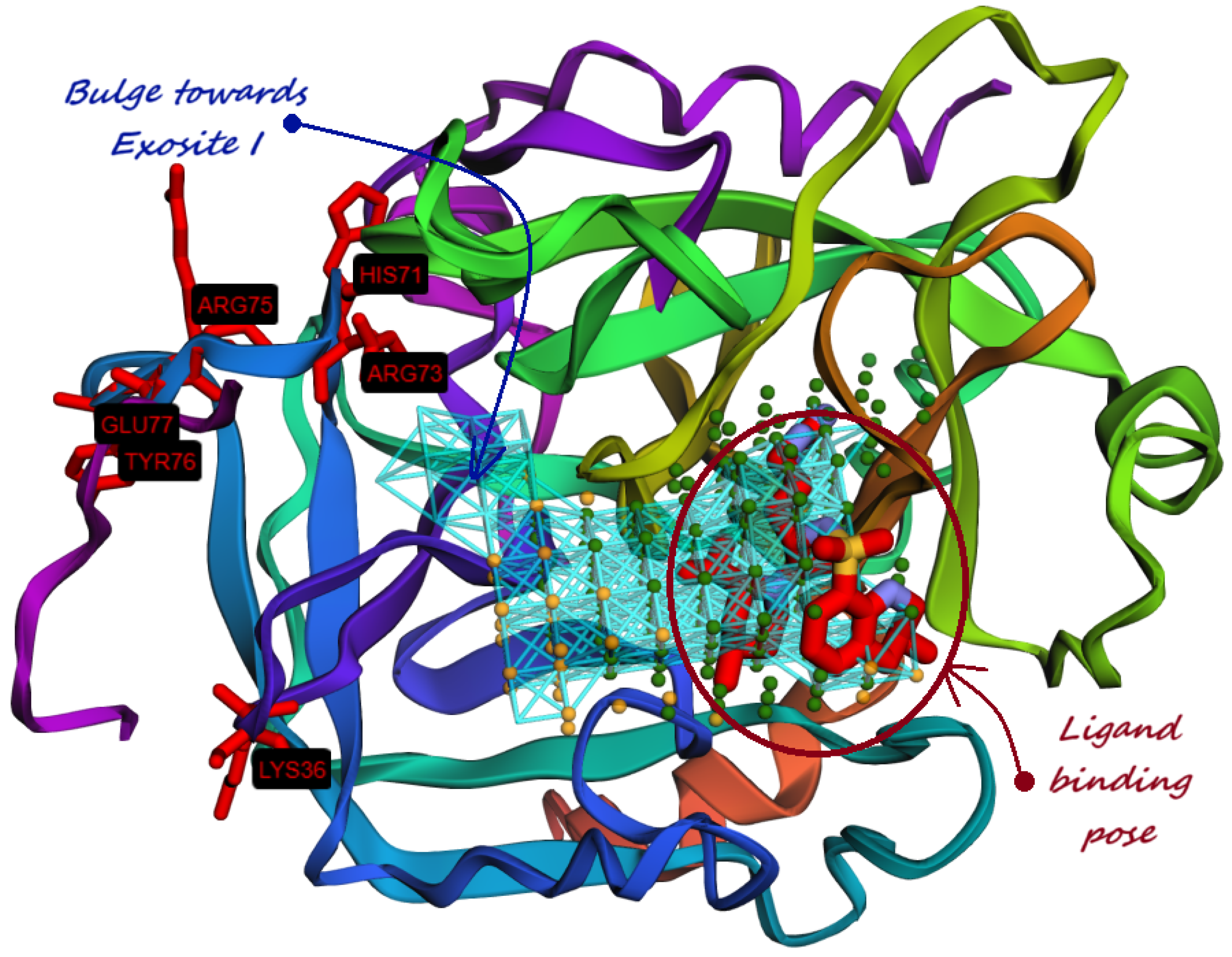
Figure 30.
Pockets predicted by Kalasanty [38] and PUResNet [36] are shown as green and orange dots, respectively. Majority-voted pockets predicted by RAPID-Net are represented by cyan sticks, while the minimally-reported pockets are shown by purple sticks. The interacting residues predicted by PUResNet V2 [33] are shown in yellow.
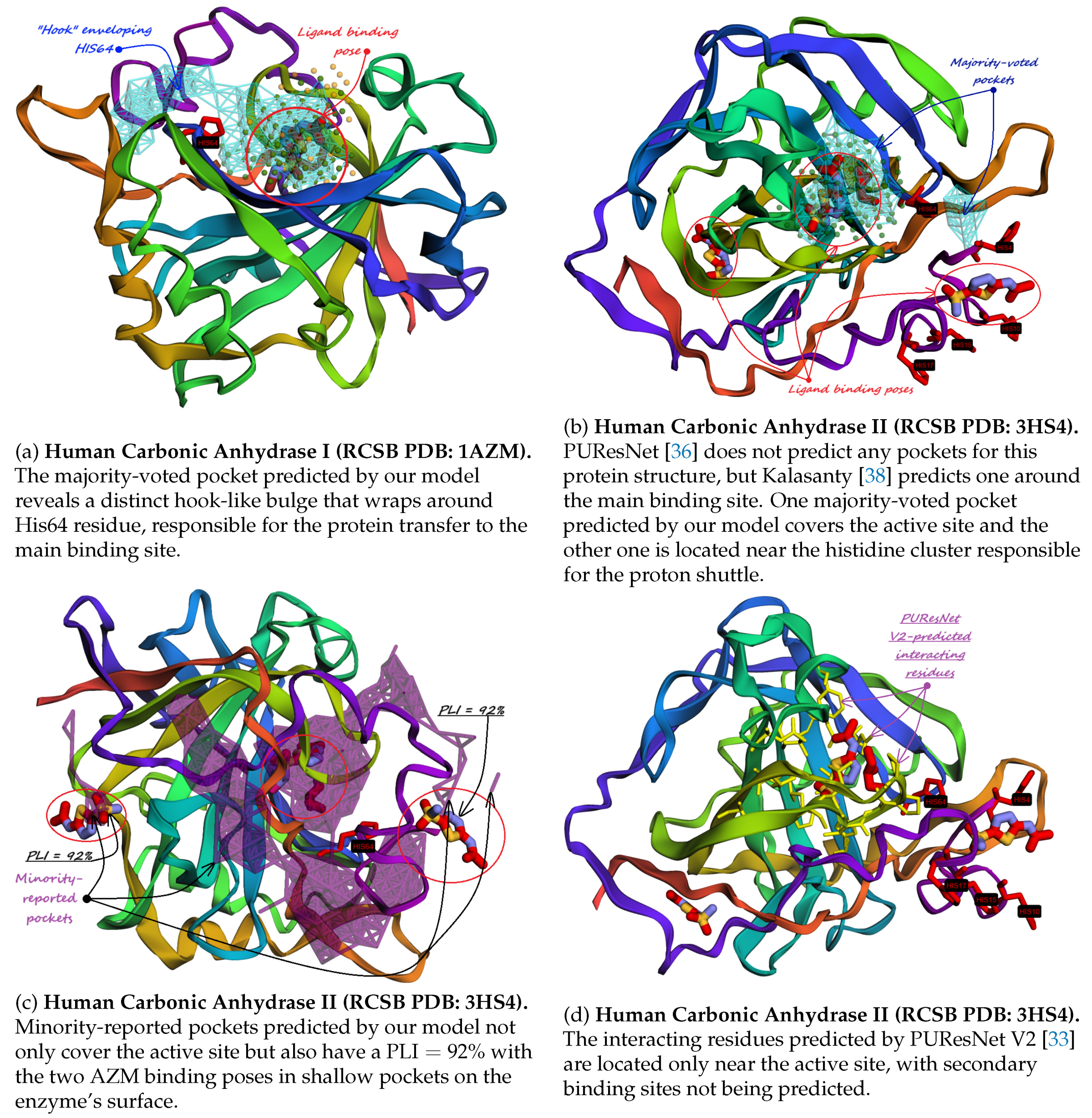
| (a) Human Carbonic Anhydrase I (RCSB PDB: 1AZM). The majority-voted pocket predicted by our model reveals a distinct hook-like bulge that wraps around His64 residue, responsible for the protein transfer to the main binding site. | (b) Human Carbonic Anhydrase II (RCSB PDB: 3HS4). PUResNet [36] does not predict any pockets for this protein structure, but Kalasanty [38] predicts one around the main binding site. One majority-voted pocket predicted by our model covers the active site and the other one is located near the histidine cluster responsible for the proton shuttle. |
| (c) Human Carbonic Anhydrase II (RCSB PDB: 3HS4). Minority-reported pockets predicted by our model not only cover the active site but also have a with the two AZM binding poses in shallow pockets on the enzyme’s surface. | (d) Human Carbonic Anhydrase II (RCSB PDB: 3HS4). The interacting residues predicted by PUResNet V2 [33] are located only near the active site, with secondary binding sites not being predicted. |
Figure 31.
Ls-AChBP (RCSB PDB: 2ZJV). The majority-voted pocket predicted by our model has a distinct bridge towards the Thr155-Asp160 region belonging to the F loop. Kalasanty [38] and PUResNet V1 [36] do not predict any pockets for this protein structure, while PUResNet V2 [33] predicts interacting residues only in the immediate vicinity of the binding pose.
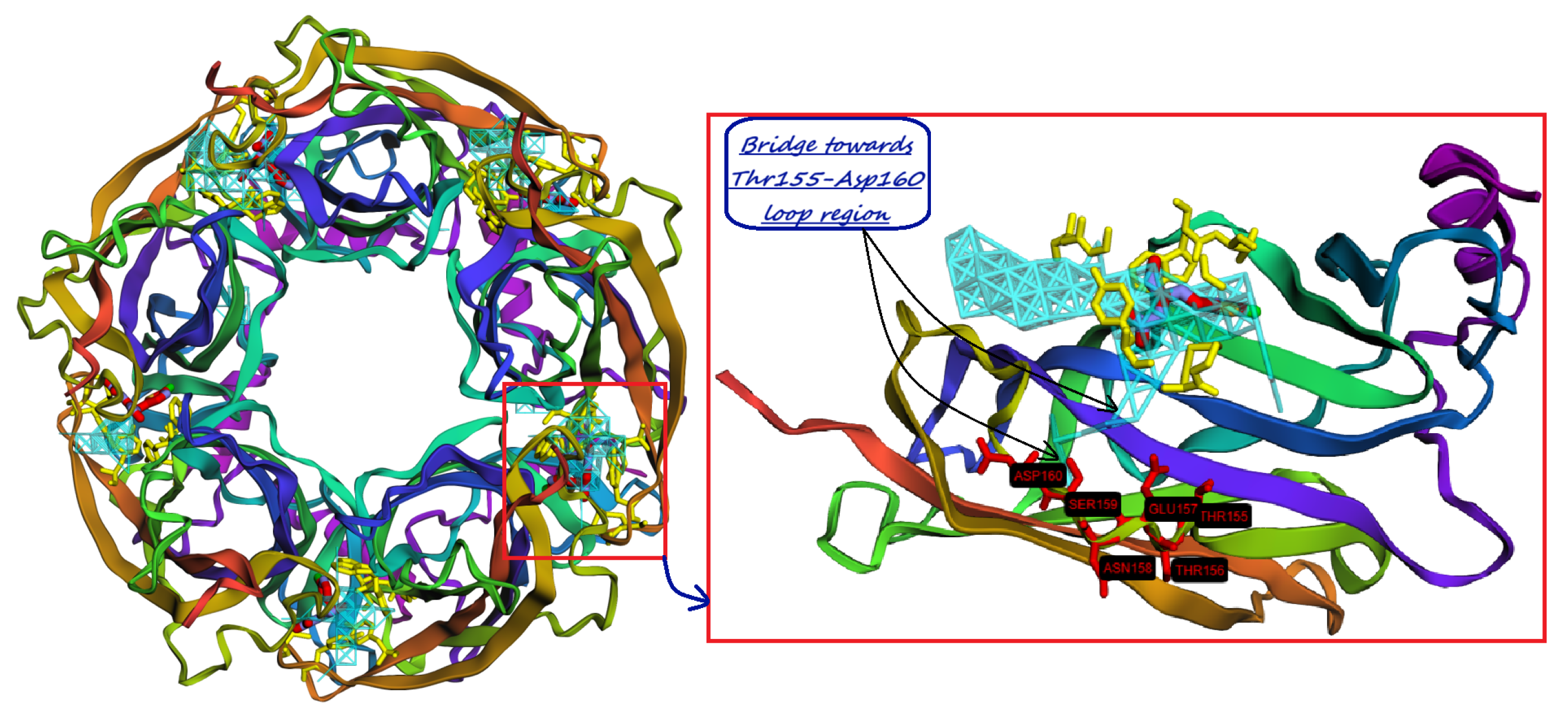

Table 1.
Comparison of pocket predictions across different methods for PoseBusters [28] dataset consisting of 308 protein structures.
Table 1.
Comparison of pocket predictions across different methods for PoseBusters [28] dataset consisting of 308 protein structures.
| Method | Nonzero | Within 15 Å | PLI |
|---|---|---|---|
| Kalasanty | 263 | 249 | 74.34% |
| PUResNet | 278 | 265 | 79.51% |
| RAPID Run 1 | 307 | 298 | 90.17% |
| RAPID Run 2 | 305 | 289 | 87.90% |
| RAPID Run 3 | 308 | 296 | 88.71% |
| RAPID Run 4 | 308 | 300 | 88.57% |
| RAPID Run 5 | 308 | 292 | 86.32% |
| RAPID ensemble | 308 | 307 | 91.44%/98.09% |
Table 2.
Comparison of pocket predictions across different methods for Astex Diverse Set [29] consisting of 85 protein structures.
Table 2.
Comparison of pocket predictions across different methods for Astex Diverse Set [29] consisting of 85 protein structures.
| Method | Nonzero | Within 15 Å | PLI |
|---|---|---|---|
| Kalasanty | 73 | 70 | 78.72% |
| PUResNet | 76 | 72 | 82.36% |
| RAPID Run 1 | 85 | 83 | 94.83% |
| RAPID Run 2 | 85 | 79 | 89.00% |
| RAPID Run 3 | 85 | 78 | 91.09% |
| RAPID Run 4 | 85 | 83 | 92.61% |
| RAPID Run 5 | 85 | 81 | 92.47% |
| RAPID ensemble | 85 | 84 | 97.15%/98.82% |
Table 3.
Comparison of pocket predictions across different methods for Coach420 [30] dataset consisting of 298 protein structures.
Table 3.
Comparison of pocket predictions across different methods for Coach420 [30] dataset consisting of 298 protein structures.
| Method | Nonzero | Within 15 Å | PLI |
|---|---|---|---|
| Kalasanty | 273 | 248 | 76.41% |
| PUResNet | 280 | 259 | 78.37% |
| RAPID Run 1 | 296 | 285 | 85.68% |
| RAPID Run 2 | 298 | 279 | 86.48% |
| RAPID Run 3 | 293 | 264 | 76.78% |
| RAPID Run 4 | 298 | 288 | 91.39% |
| RAPID Run 5 | 298 | 275 | 80.59% |
| RAPID ensemble | 298 | 297 | 86.75%/95.49% |
Table 4.
Comparison of pocket predictions across different methods for BU48 [31] dataset consisting of 62 protein structures.
Table 4.
Comparison of pocket predictions across different methods for BU48 [31] dataset consisting of 62 protein structures.
| Method | Nonzero | Within 15 Å | PLI |
|---|---|---|---|
| Kalasanty | 54 | 53 | 77.80% |
| PUResNet | 42 | 39 | 46.90% |
| RAPID Run 1 | 61 | 60 | 86.52% |
| RAPID Run 2 | 62 | 62 | 97.57% |
| RAPID Run 3 | 61 | 60 | 86.68% |
| RAPID Run 4 | 60 | 58 | 84.47% |
| RAPID Run 5 | 62 | 43 | 46.97% |
| RAPID ensemble | 62 | 62 | 95.79%/99.82% |
Disclaimer/Publisher’s Note: The statements, opinions and data contained in all publications are solely those of the individual author(s) and contributor(s) and not of MDPI and/or the editor(s). MDPI and/or the editor(s) disclaim responsibility for any injury to people or property resulting from any ideas, methods, instructions or products referred to in the content. |
© 2025 by the authors. Licensee MDPI, Basel, Switzerland. This article is an open access article distributed under the terms and conditions of the Creative Commons Attribution (CC BY) license (http://creativecommons.org/licenses/by/4.0/).
Copyright: This open access article is published under a Creative Commons CC BY 4.0 license, which permit the free download, distribution, and reuse, provided that the author and preprint are cited in any reuse.


