Starobinsky Inflation with T-Model Kähler Geometries

1. Introduction

Starobinsky inflation (SI) [1] stands out among the remaining viable inflationary models (for reviews see Refs. [2,3,4,5]) thanks to its simplicity, elegance and observational success. Despite its original realization by the (arbitrary) addition of the ${\mathcal{R}}^2$ term – where $\mathcal{R}$ is the Ricci scalar – to the standard Einstein action, this inflationary model can be also driven by a scalar field with a suitable potential. Indeed, it is well known that gravity theories based on higher derivative terms of the type ${\mathcal{R}}^m$ with $m>1$ are equivalent to standard gravity theories with one additional scalar degree of freedom [6]. From the proposed particle-physics incarnations of this inflationary model (and its variant called $\alpha$-SI) – for reviews see Refs. [7,8,9,10] – prominent position occupies its embedding within Supergravity (SUGRA) which is the natural extension of Supersymmetry (SUSY) to planckian mass scales [11]. Despite the fact that SUSY is not yet discovered at LHC [12], its presence – probably at higher energies – is a natural and mostly inevitable consequence of superstring theory [13]. Even without direct experimental signatures, SUSY has constructive impact on the stabilization of the electroweak vacuum and on several problems of modern Particle Cosmology such as inflation, baryogenesis and dark matter.

Trying to classify the most popular SUGRA realizations of SI we can single out indicatively the following categories – for alternatives see, e.g., Refs. [6,14,15,16,17,18]:

• Wess-Zumino models with a matter-like inflaton [19,20,21,22,23,24]. Polynomial superpotentials, W, – of the Wess-Zumino form [11] – are adopted in this class of models and the Kähler potentials K parameterize specific Kähler manifolds of the form $SU(N_{\mathrm{m}},1)/SU\left(N_{\mathrm{m}}\right)\times U\left(1\right)$, inspired by the no-scale models [25,26] of SUSY breaking. The stabilization of the inflaton-accompanying modulus at a Planck-scale value [20] is achieved by a deformation of the internal geometry.
• Ceccoti-like [27] models with a modulus-like inflaton [20,28,29,30,31,32,33,34,35,36,37]. Similar K’s are used here whereas W is linear [38] with respect to the matter-like inflaton-accompanying field which may be stabilized at the origin via several mechanisms [6,10,35,39,40,41,42,43]. In a subclass of these models [31,32,33,34,36,37], the conjecture of induced gravity [44,45] is incorporated leading to a dynamical generation of the reduced Planck scale, $m_{\mathrm{P}}$ through the vacuum expectation value (v.e.v) of the inflaton at the end of its evolution.
• Models with a strong linear non-minimal coupling to gravity [46,47,48] – or a strong linear contribution into this coupling [49] – which remain unitarity safe [50] up to the Planck scale.
• Models which exhibit a pole [51,52,53,54,55] of order one in the kinetic term of the inflaton [56,57,58]. As in every SI model, the inflationary potential develops one shoulder for large $\widehat{\varphi }$ values, where $\widehat{\varphi }$ is the canonically normalized inflaton which can be expressed in terms of the original field $\varphi$ as [58]

  $$\varphi =1-e^{-\sqrt{2/N}\widehat{\varphi }}(:\mathrm{E-Model} \mathrm{Normalization}).$$

  (1.1)
  The presence of the real positive variable N – aligned with the conventions of [58] – leads to a generalized version of SI called $\alpha$-SI [20] or E-Model inflation. This model can be contrasted with the T-Model inflation [59,60] which arises thanks to a pole of order two in the inflaton kinetic term and features a potential with two symmetric plateaus away from the origin. Namely, the $\varphi -\widehat{\varphi }$ relation assumes the form

  $$\varphi =tanh\left(\widehat{\varphi }/\sqrt{2N}\right)(:\mathrm{T-Model} \mathrm{Normalization}).$$

  (1.2)
  Independently of their particularities, both models share [8] common predictions for the inflationary observables and for this reason they are called collectively $\alpha$-attractors [5,61,62,63].

In our present investigation, stimulated by Ref. [60] – see also Ref. [64] –, we propose another embedding of SI within $\mathcal{N}=1$ standard Poincaré SUGRA which is exclusively based on the presence of a pole of order two in the inflaton kinetic term, i.e., it is based on the $\varphi -\widehat{\varphi }$ relation of Eq. (1.2). Namely, the scalar potential, expressed in terms of the initial (non-canonical) inflaton, $\varphi$, is written as

$$V_{\mathrm{I}}={\lambda }^2{({\varphi }^{n/2}-M^2)}^2/{(1+\varphi )}^{n_{\mathrm{d}}}withM\ll m_{\mathrm{P}}=1.$$

(1.3)

For $n=n_{\mathrm{d}}=2$, $V_{\mathrm{I}}$ has been motivated in Refs. [29,60] via a breaking of conformal symmetry in a non-SUSY framework. It also appears in unified models of no-scale $\alpha$-SI with SUSY breaking [65]. Here we extend the analysis in the context of SUGRA providing a method which allows the generation of $V_{\mathrm{I}}$ from conveniently selected W and K. Our particle content includes besides the inflaton superfield(s) an extra gauge singlet superfield which assist in the stabilization of the SUGRA potential during SI [38]. Moreover, we employ monomial W’s consistent with an R and a global or gauge $U{\left(1\right)}_X$ symmetry. On the other hand, the K’s respect the R and the gauge symmetry and are holomorphically equivalent to those yielding Eq. (1.2) [56,66,67,68]. In other words, K has the well-known form employed in T-model inflation [56,66] up to a number of extra holomorphic and anti-holomorphic terms which do not influence the resulting Kähler metric. The one pair of these terms endows K with a shift symmetry which facilitates the performance of inflation – cf. Refs. [56,66,67,68]. The second pair provides a breaking of the aforementioned shift symmetry which is already violated mildly in W. Both violations are natural in the ’t Hooft sense [69] for low enough values of the exponent $n_{\mathrm{d}}$ in K and the coupling constant $\lambda$ entered in W. The particular importance of an enhanced shift symmetry in taming the so-called $\eta$-problem of inflation in SUGRA is already recognized for gauge singlets, e.g., in [70,71,72,73,74,75] and non-singlets, e.g., in Refs. [36,48,76,77,78,79].

Compared to the aforementioned implementations of SI within SUGRA, the present version assures a totally symmetric Kähler manifold together with a simple W. Let us recall that polynomial W’s with R symmetry are reconciled with a K which does not parameterize specific Kähler manifold in Ref. [58] whereas totally symmetric K’s usually require complicate W’s – see e.g. Refs. [20,30,56,57,61]. On the contrary, the employed here W’s are very common in particle physics and so the inflaton can be easily identified with a field already present in the theory, e.g, the right-handed sneutrino [70,80,81] or a superheavy Higgs superfield responsible for the spontaneous breaking of a gauge symmetry [36,37]. Also, it is expected that this scheme assures naturally a low enough reheating temperature, potentially consistent with the gravitino constraint and non-thermal leptogenesis [31,36,37,83,84] if connected with a version of the Minimal SUSY Standard Model (MSSM). Furthermore, our proposal does not require tuning of parameters – besides a mild one in the initial conditions –, it is not based on any conjecture such as that of induced gravity [10,31,32,33,34,35,36,37] and provides a relative flexibility as regards the observables. At last, it offers us the opportunity to exemplify the Kähler potential engineering which allows to obtain the various desired factors of $V_{\mathrm{I}}$ in Eq. (1.3) together with a desirable Kähler metric.

We below describe how we can formulate SI in the context of SUGRA in Section 2 and we specify two versions of SI: one employing a gauge-singlet inflaton in Section 3 called for short Chaotic Starobinsky Inflation (CSI) and one with a gauge non-singlet inflaton leading to the breaking of a gauge group called Higgs Starobinsky Inflation (HSI) in Section 4. Our conclusions are summarized in Section 6. In Appendix A we demonstrate that our proposed K’s enjoy an enhanced shift symmetry. Throughout the text, the subscript $,\chi$ denotes derivation with respect to (w.r.t) the field $\chi$ and charge conjugation is denoted by a star (^*). Unless otherwise stated, we use units where the reduced Planck scale $m_{\mathrm{P}}=2.4·{10}^{18}\mathrm{GeV}$ is set equal to unity.

2. SUGRA Framework

We start our investigation presenting the basic formulation of a scalar theory within SUGRA in Section 2.1 and then – in Section 2.2 – we outline our strategy in constructing our models of SI.

2.1. General Set-Up

The part of the (Einstein-frame) action within SUGRA which describes the (complex) scalar fields $z^{\alpha }$ coupled minimally to Einstein gravity can be written as [11]

$$\mathcal{A}=\int d^{4}x\sqrt{-\mathfrak{g}}\left(-{\displaystyle \frac{1}{2}}\mathcal{R}+K_{\alpha \overline{\beta }}{D}_{\mu }{z}^{\alpha }{D}^{\mu }{z}^{*\overline{\beta }}-V_{\mathrm{SUGRA}}\right),$$

(2.1a)

where $\mathcal{R}$ is the space-time Ricci scalar curvature, $\mathfrak{g}$ is the determinant of the Friedmann-Robertson-Walker metric, $g_{\mu \nu }$, with signature $(+,-,-,-)$. Also, summation is taken over the scalar fields $z^{\alpha }$, the kinetic mixing of which is controlled by the Kähler potential K and the relevant metric defined as

$$K_{\alpha \overline{\beta }}=K_{,z^{\alpha }{z}^{*\overline{\beta }}}>0with{K}^{\overline{\beta }\alpha }{K}_{\alpha \overline{\gamma }}={\delta }_{\overline{\gamma }}^{\overline{\beta }}.$$

(2.1b)

Also, the covariant derivatives for the $z^{\alpha }$’s are given by

$$D_{\mu }{z}^{\alpha }={\partial }_{\mu }{z}^{\alpha }+ig{A}_{\mu }^{\mathrm{a}}{T}_{\alpha \beta }^{\mathrm{a}}{z}^{\beta }$$

(2.1c)

with $A_{\mu }^{\mathrm{a}}$ being the vector gauge fields, g the (unified) gauge coupling constant and $T^{\mathrm{a}}$ with $\mathrm{a}=1,...,\mathsf{dim}{G}_{\mathrm{GUT}}$ the generators of a gauge group $G_{\mathrm{GUT}}$. Here and henceforth, the scalar components of the various superfields are denoted by the same superfield symbol.

Finally $\mathcal{A}$ contains the SUGRA scalar potential, $V_{\mathrm{SUGRA}}$, which is given in terms of K, and the superpotential, W, by

$$V_{\mathrm{SUGRA}}=V_{\mathrm{F}}+V_{\mathrm{D}}with{V}_{\mathrm{F}}=e^K\left(K^{\alpha \overline{\beta }}{\mathrm{F}}_{\alpha }{\mathrm{F}}_{\overline{\beta }}^{*}-3{\left|W\right|}^2\right)and{V}_{\mathrm{D}}=g^2\sum _{\mathrm{a}}{\mathrm{D}}_{\mathrm{a}}{\mathrm{D}}_{\mathrm{a}}/2,$$

(2.1d)

dwhere a trivial gauge kinetic function is adopted whereas the F- and D-terms read

$${\mathrm{F}}_{\alpha }=W_{,z^{\alpha }}+K_{,z^{\alpha }}Wand{\mathrm{D}}_{\mathrm{a}}=z_{\alpha }{\left(T_{\mathrm{a}}\right)}_{\beta }^{\alpha }{K}^{\beta }with{K}^{\alpha }=K_{,z^{\alpha }}.$$

(2.1e)

As we emphasized in Section 1, SI in our work is attained by deriving $V_{\mathrm{I}}$ in Eq. (1.3) from $V_{\mathrm{SUGRA}}$ and not modifying gravity which remains at the minimal level as shown from the absence of higher order $\mathcal{R}$ terms in Eq. (2.1a). Therefore our next task is to select conveniently the functions K and W so that Eqs. (1.2) and (1.3) are reproduced.

2.2. Guidelines

We embark on describing our procedure to obtain the desired $V_{\mathrm{I}}$ in Eq. (1.3) from $V_{\mathrm{F}}$ in Eq. (2.1d) and the desired $\varphi -\widehat{\varphi }$ relation in Eq. (1.2). Although our presentation in adapted to our present model, the strategy of our approach has a wider applicability suitable for other cases too.

2.2.1. Achieving D-Flatness.

Our final aim is the derivation of $V_{\mathrm{I}}$ in Eq. (1.3) through $V_{\mathrm{F}}$ in Eq. (2.1d). This decision requires the establishment of D-flatness during SI, i.e., ${\langle V_{\mathrm{D}}\rangle }_{\mathrm{I}}=0$ – where ${\langle Q\rangle }_{\mathrm{I}}$ symbolizes the value of the quantity Q during inflation. Assuming that the gauge non-singlet superfields are placed at zero during inflation, D-flatness may be attained in the following two cases:

• If the inflaton is (the radial part of) a gauge-singlet superfield $z^2:=\Phi$. In this case, $\Phi$ has obviously zero contribution to $V_{\mathrm{D}}$.
• If the inflaton is the radial part of a conjugate pair of Higgs superfields, $z^2:=\Phi$ and $z^3:=\overline{\Phi }$, in the fundamental representation of $G_{\mathrm{GUT}}$. In a such case – see Section 4.3 below – we obtain ${\langle V_{\mathrm{D}}\rangle }_{\mathrm{I}}=0$. The same result can be obtained if $G_{\mathrm{GUT}}$ is more structured than $U{\left(1\right)}_X$ employing just one superfield $z^2$ in the adjoint representation of $G_{\mathrm{GUT}}$ and using as inflaton its neutral component – see e.g. Ref. [85].

2.2.2. Selecting the Suitable W

Despite the fact that $V_{\mathrm{I}}$ in Eq. (1.3) includes only one field, its derivation from $V_{\mathrm{F}}$ is facilitated [38] if W includes at least two fields from which the first $z^1:=S$ is a gauge-singlet superfield, called stabilizer or goldstino. The latter is due to the fact that for $S=0$ SUSY is broken since ${\langle F_S\rangle }_{\mathrm{I}}\ne 0$. The presence of S serves the following purposes:

• It assists in determining W. To achieve it, we require that S appears linearly in W and so both are equally charged under a global R symmetry.
• It can be stabilized at ${\langle S\rangle }_{\mathrm{I}}=0$ without invoking higher order terms, if we select [35]

  $$K_2=N_{S}ln\left(1+{\left|S\right|}^2/N_S\right)\Rightarrow {\langle K_2^{S{S}^{*}}\rangle }_{\mathrm{I}}=1with0<N_2<6.$$

  (2.2)
  The index 2 stems from the fact that $K_{\mathrm{s}}$ parameterizes the compact manifold $SU\left(2\right)/U\left(1\right)$ [35]. Note that for ${\langle S\rangle }_{\mathrm{I}}=0$, S is canonically normalized and so we do not care about its kinetic normalization henceforth. For other stabilization methods of S see Refs. [6,39,40,41,42,43].
• It assures the boundedness of $V_{\mathrm{I}}$. Indeed, if we set ${\langle S\rangle }_{\mathrm{I}}=0$, then ${\langle W_{,z^{\alpha }}\rangle }_{\mathrm{I}}=0$ for $\alpha \ne 1$, ${\langle K_{,z^{\alpha }}W\rangle }_{\mathrm{I}}=0$ and ${-3|\langle W\rangle }_{\mathrm{I}}{|}^2=0$. Obviously, non-vanishing values of the last term may render $V_{\mathrm{F}}$ unbounded from below.
• It generates for ${\langle S\rangle }_{\mathrm{I}}=0$ and for monomial W the numerator of $V_{\mathrm{I}}$ in Eq. (1.3) via the only term of $V_{\mathrm{F}}$ which remains “alive”. Indeed, we obtain

  $$V_{\mathrm{I}}:={\langle V_{\mathrm{F}}\rangle }_{\mathrm{I}}={\langle e^K{K}^{S{S}^{*}}{\left|W_{,S}\right|}^2\rangle }_{\mathrm{I}}.$$

  (2.3)
  Assuming that no mixing terms between S and the inflaton exist in K, we obtain ${\langle K^{S{S}^{*}}\rangle }_{\mathrm{I}}={\langle K_2^{S{S}^{*}}\rangle }_{\mathrm{I}}=1$ and so the numerator of $V_{\mathrm{I}}$ in Eq. (1.3) emerges if W has the form

  $$W=S{F}_{\mathrm{W}}\left(z^{\alpha }\right)with{\langle F_{\mathrm{W}}\rangle }_{\mathrm{I}}=:f_{\mathrm{W}}=\lambda {\varphi }^{n/2}and\varphi =\mathsf{Re}\Phi ,$$

  (2.4)

  given that the assumption ${\langle \mathsf{Im}\Phi \rangle }_{\mathrm{I}}=0$ yields mostly stable configuration – here we focus on a gauge-singlet $\Phi$. On the other hand, the denominator of $V_{\mathrm{I}}$ in Eq. (1.3) may be generated via the exponential prefactor in Eq. (2.3) through logarithmic contributions to K – as we explain below.

2.2.3. Selecting the Convenient Kähler  Potential

The form of K has to accomplish the following two goals:

• It has to generate the desired $\varphi -\widehat{\varphi }$ relation in Eq. (1.2). Therefore, we need to introduce a contribution into K including $z^{\alpha }$ and $z^{*\alpha }$ in the same function. After inspection – see Appendix of Ref. [86] – we infer that a pole of order two in the kinetic term of inflaton is achieved if $K=K_{\mathrm{T}}$ where

  $$K_{\mathrm{T}}=-Nln{F}_{\mathrm{T}}(z^{\alpha },z^{*\overline{\beta }})with{\langle K_{\alpha \overline{\beta }}\rangle }_{\mathrm{I}}=N/f_{\mathrm{T}}^{2}and{f}_{\mathrm{T}}:={\langle F_{\mathrm{T}}\rangle }_{\mathrm{I}}=1-{\varphi }^2.$$

  (2.5)
  Here $N>0$ and the subscript “T” indicates that this part of the total K is responsible for the T-model Kähler metric – see Eq. (2.1b). However, from Eq. (2.3), we remark that K affects – besides the kinetic mixing – $V_{\mathrm{I}}$ via the prefactor $e^{K_{\mathrm{T}}}$. Therefore, $F_{\mathrm{T}}$ is generically expected to emerge also in the denominator of $V_{\mathrm{I}}$ making difficult the establishment of an inflationary era. This problem can be surpassed [58,66] by two alternative strategies:

  -

  Adjusting W and constraining the prefactor of K in Eq. (2.5), so that the pole is removed from $V_{\mathrm{F}}$ thanks to cancellations [19,54,58,66]. This recipe introduces some tuning, though, in the coefficients of W and, for this reason, we do not pursue this method here.

  -

  Replacing $K_{\mathrm{T}}$ with ${\tilde{K}}_{\mathrm{T}}$ so that the desired kinetic terms in Eq. (2.1a) remain unaltered and, simultaneously [56,58,66]

  $${\langle e^{{\tilde{K}}_{\mathrm{T}}}\rangle }_{\mathrm{I}}=1\iff {\langle {\tilde{K}}_{\mathrm{T}}\rangle }_{\mathrm{I}}=0with{\tilde{K}}_{\mathrm{T}}=K_{\mathrm{T}}+K_{\mathrm{sh}}.$$

  (2.6a)

  In other words, the symmetry of $K_{\mathrm{T}}$ is augmented by some shift symmetry – see Appendix A – without disturbing $K_{\alpha \overline{\beta }}$ in Eq. (2.1b). To accomplish this, $K_{\mathrm{sh}}$ includes holomorphic and anti-holomorphic terms which yield vanishing contribution to the mixed derivatives of ${\tilde{K}}_{\mathrm{T}}$. Taking into account the form of $K_{\mathrm{T}}$ in Eq. (2.5), we may select formally

  $$K_{\mathrm{sh}}=(N/2)ln{F}_{\mathrm{sh}}+(N/2)ln{F}_{\mathrm{sh}}^{*}with{\langle F_{\mathrm{sh}}\rangle }_{\mathrm{I}}=:f_{\mathrm{sh}}=f_{\mathrm{T}}.$$

  (2.6b)

  Note that the same construction is valid even in case of polynomial K’s if we check the structure of the relevant K’s in Refs. [70,74,75,76,77,78,79].

• It has to generate the denominator of $V_{\mathrm{I}}$ in Eq. (1.3). To achieve this, we focus on the exponential prefactor of $V_{\mathrm{I}}$ in Eq. (2.3) and we demand

  $${\langle e^{K_{\mathrm{d}}}\rangle }_{\mathrm{I}}={(1+\varphi )}^{-n_{\mathrm{d}}},$$

  (2.7a)

  where $K_{\mathrm{d}}$ has the following structure (similar to that of $K_{\mathrm{sh}}$)

  $$K_{\mathrm{d}}=-(n_{\mathrm{d}}/2)ln{F}_{\mathrm{d}}-(n_{\mathrm{d}}/2)ln{F}_{\mathrm{d}}^{*}with{\langle F_{\mathrm{d}}\rangle }_{\mathrm{I}}=:f_{\mathrm{d}}=1+\varphi .$$

  (2.7b)

  bso that it does not disrupt $K_{\alpha \overline{\beta }}$ in Eq. (2.1b).

To recapitulate this section, we summarize that the adopted W in this work has the form in Eq. (2.4) whereas the total K can be written as

$${\tilde{K}}_{2\mathrm{Td}}=K_2+{\tilde{K}}_{\mathrm{T}}+K_{\mathrm{d}}with{\tilde{K}}_{\mathrm{T}}=K_{\mathrm{T}}+K_{\mathrm{sh}}.$$

(2.8)

Below, we specify the functional forms of the related functions $F_{\mathrm{T}},F_{\mathrm{sh}}$ and $F_{\mathrm{d}}$ for the two classes of SI considered, CSI and HSI.

3. Gauge-Singlet Inflaton

We focus first on the case of CSI and we present in Section 3.1 the building blocks of the model. Then we verify that the adopted K and W produce the desired kinetic mixing in Section 3.2 and inflationary potential in Section 3.3.

3.1. Set-Up

According to the strategy described in Section 2.2 the present setting is realized in presence of two gauge-singlet superfields S and $\Phi$ which may be parameterized as

$$\Phi =\varphi e^{i\theta }andS=(s+i\overline{s})/\sqrt{2}.$$

(3.1)

The inflationary trajectory can be defined by the constraints

$${\langle S\rangle }_{\mathrm{I}}={\langle \Phi -{\Phi }^{*}\rangle }_{\mathrm{I}}=0,or{\langle s\rangle }_{\mathrm{I}}={\langle \overline{s}\rangle }_{\mathrm{I}}={\langle \theta \rangle }_{\mathrm{I}}=0.$$

(3.2)

Following our plan in Section 2.2.2 we adopt a monomial W consistent with Eq. (2.4) with the following structure

$$F_{\mathrm{W}}=\lambda {\Phi }^{n/2}\mathrm{and}\mathrm{so}W=\lambda S{\Phi }^{n/2},$$

(3.3)

where $\lambda$ is a free parameter and n takes even values which preserve the holomorphicity of W. The form of W can be uniquely determined if we impose an R symmetry, under which S and $\Phi$ have charges 1 and 0, and a global $U{\left(1\right)}_X$ symmetry with assigned charges $Q_X\left(S\right)=-1$ and $Q_X(\Phi )=2/n$. The latter is violated though in the proposed K which assumes the form in Eq. (2.8) with the functions defined in Eqs. (2.5), (2.6b) and (2.7b) identified as follows

$$F_{\mathrm{T}}=1-{|\Phi |}^2,F_{\mathrm{sh}}=1-{\Phi }^{2}and{F}_{\mathrm{d}}=1+\Phi .$$

(3.4)

Consequently, the total K takes the form

$${\tilde{K}}_{211\mathrm{d}}=K_2+{\tilde{K}}_{11}+K_{\mathrm{d}},$$

(3.5)

where the individual contributions are specified as

$${\tilde{K}}_{11}=-Nln{\displaystyle \frac{1-{|\Phi |}^2}{\sqrt{(1-{\Phi }^2)(1-{\Phi }^{*2})}}}and{K}_{\mathrm{d}}=-{\displaystyle \frac{n_{\mathrm{d}}}{2}}ln(1+\Phi )-{\displaystyle \frac{n_{\mathrm{d}}}{2}}ln(1+{\Phi }^{*}).$$

(3.6)

${\tilde{K}}_{211\mathrm{d}}$ parameterizes [56] the Kähler manifold ${\mathcal{M}}_{211}$ with moduli-space scalar curvature ${\mathsf{R}}_{211}$ given respectively by

$${\mathcal{M}}_{211}={(SU\left(2\right)/U\left(1\right))}_S\times {\left(SU(1,1)/U\left(1\right)\right)}_{\Phi }and{\mathsf{R}}_{211}=-2/N+2/N_S.$$

(3.7)

The indices in the product of Eq. (3.7) indicate the moduli which parameterize the corresponding manifolds. Needless to say, $K_{\mathrm{d}}$ and the denominator in ${\tilde{K}}_{11}$ have no impact on ${\mathcal{M}}_{211}$, as explained in Section 2.2.3, and violate the global $U{\left(1\right)}_X$ symmetry which is valid at the level of W.

3.2. Canonical Normalization

The first step towards the establishment of CSI is the canonical normalization of the fields involved in the parametrization of $\Phi$ in Eq. (3.1). This can be done if we identify the kinetic term on Eq. (2.1a) with the canonical ones as follows

$${\langle K_{\Phi {\Phi }^{*}}\rangle }_{\mathrm{I}}{\left|\dot{\Phi }\right|}^2\simeq {\displaystyle \frac{1}{2}}\left({\dot{\widehat{\varphi }}}^2+{\dot{\widehat{\theta }}}^2\right)\Rightarrow {\displaystyle \frac{d\widehat{\varphi }}{d\varphi }}=J={\displaystyle \frac{\sqrt{2N}}{f_{\mathrm{T}}}}and\widehat{\theta }\simeq J\varphi \theta with{\langle K_{\Phi {\Phi }^{*}}\rangle }_{\mathrm{I}}={\displaystyle \frac{N}{f_{\mathrm{T}}^2}},$$

(3.8)

found from Eq. (A3) if we restrict our attention on the path in Eq. (3.2). Upon integrating the $\varphi -\widehat{\varphi }$ relation above we arrive at Eq. (1.2) in accordance with our aim.

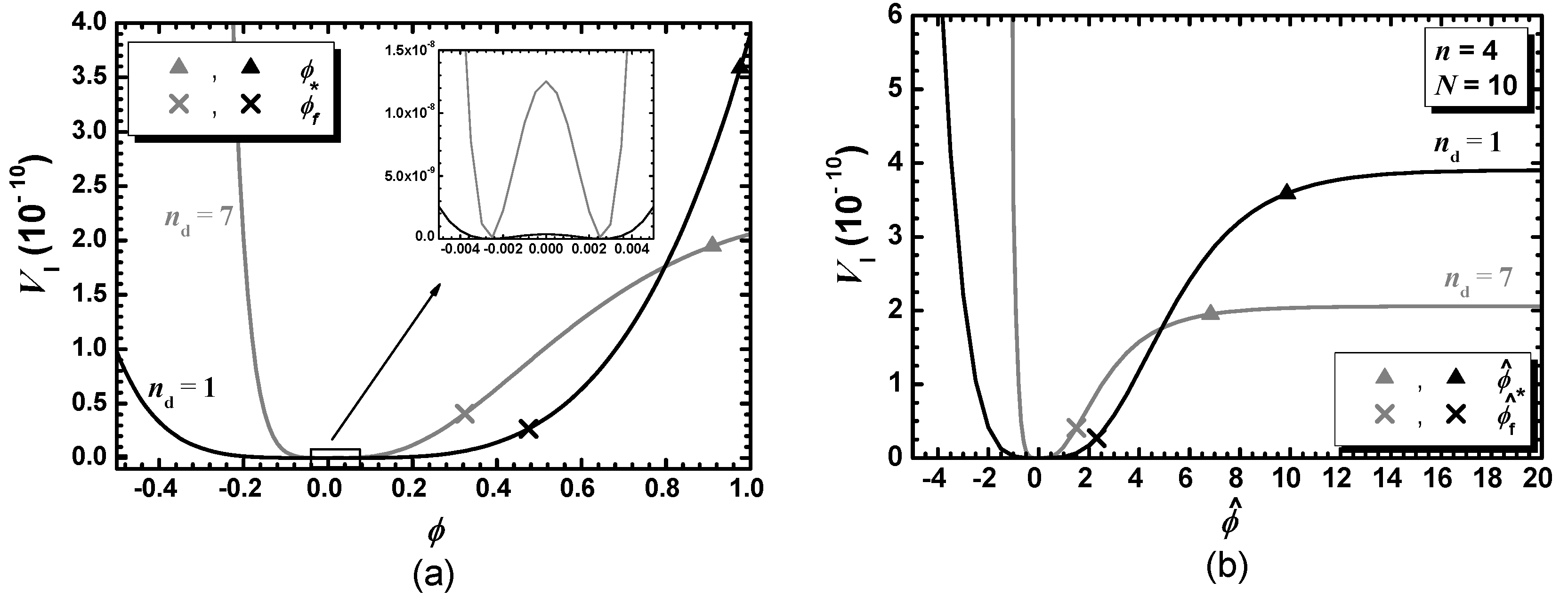
3.3. Inflationary Potential

The second step in our attempt to implement SI is the reproduction of $V_{\mathrm{I}}$ of Eq. (1.3) starting from Eq. (2.3) with W given in Eq. (3.3) and $K={\tilde{K}}_{211\mathrm{d}}$ in Eq. (3.5). This is trivially verified if we take into account the field configuration of Eq. (3.2). However, $V_{\mathrm{I}}$ of Eq. (1.3) is a tree-level result which may receive radiative corrections. These can be estimated by constructing the mass spectrum of the theory along the trajectory in Eq. (3.2). Our results are summarized in Table 1, where we arrange the expressions of the masses squared ${\widehat{m}}_{{\chi }^{\alpha }}^2$ (with ${\chi }^{\alpha }=\theta$ and s) divided by $H_{\mathrm{I}}^2\simeq V_{\mathrm{I}}/3$. From them we can appreciate the role of $N_S<6$ in retaining positive ${\widehat{m}}_s^2$ and thereby stabilizing the track in Eq. (3.2). Also, we confirm that ${\widehat{m}}_{{\chi }^{\alpha }}^2\gg H_{\mathrm{I}}^2$ for $\varphi \le 1$ and so we do not obtain inflationary primordial perturbation from other fields besides $\varphi$. In Table 1 we display also the masses ${\widehat{m}}_{\psi \pm }^2$ of the corresponding fermions too – we define ${\widehat{\psi }}_{\Phi }=J{\psi }_{\Phi }$ where ${\psi }_{\Phi }$ and ${\psi }_S$ are the Weyl spinors associated with S and $\Phi$ respectively. Considering SUGRA as an effective theory with cutoff scale equal to $m_{\mathrm{P}}$, the well-known Coleman-Weinberg formula – see e.g [77] – can be employed self-consistently taking into account the masses which lie well below $m_{\mathrm{P}}$, i.e., all the masses arranged in Table 1. Therefore, the one-loop correction to $V_{\mathrm{I}}$ reads

$$\Delta V_{\mathrm{I}}={\displaystyle \frac{1}{64{\pi }^2}}\left({\widehat{m}}_{\theta }^{4}ln{\displaystyle \frac{{\widehat{m}}_{\theta }^2}{{\Lambda }^2}}+2m_s^{4}ln{\displaystyle \frac{m_s^2}{{\Lambda }^2}}-4{\widehat{m}}_{{\psi }_{\pm }}^{4}ln{\displaystyle \frac{{\widehat{m}}_{{\psi }_{\pm }}^2}{{\Lambda }^2}}\right),$$

(3.9)

where $\Lambda$ is a renormalization group (RG) mass scale. The resulting $\Delta V_{\mathrm{I}}$ lets intact our inflationary outputs, provided that $\Lambda$ is determined by requiring $\Delta V_{\mathrm{I}}\left({\varphi }_{★}\right)=0$ or $\Delta V_{\mathrm{I}}\left({\varphi }_{\mathrm{f}}\right)=0$. Namely, solving these conditions w.r.t $\Lambda$ we obtain

$$\Lambda =e^{c_m/c_{\Lambda }}with\left\{\begin{array}{c}{c}_m={\widehat{m}}_{\theta }^{4}ln{\widehat{m}}_{\theta }^2+2m_s^{4}ln{m}_s^2-4{\widehat{m}}_{{\psi }_{\pm }}^{4}ln{\widehat{m}}_{{\psi }_{\pm }}^2,\hfill \\ c_{\Lambda }={\widehat{m}}_{\theta }^4+2m_s^4-4{\widehat{m}}_{{\psi }_{\pm }}^4.\hfill \end{array}\right.$$

(3.10)

If determined for $\varphi ={\varphi }_{★}$ or $\varphi ={\varphi }_{\mathrm{f}}$, the expression above yields ${\Lambda }_{★}=\Lambda \left({\varphi }_{★}\right)$ or ${\Lambda }_{\mathrm{f}}=\Lambda \left({\varphi }_{\mathrm{f}}\right)$. Both choices let intact the inflationary observables derived exclusively by using the (tree level) $V_{\mathrm{I}}$ in Eq. (1.3) as shown for a similar model in Ref. [77]. Moreover, the renormalization-group running is expected to be negligible because $\Lambda$ is close to the inflationary scale $H_{\mathrm{I}}$ – see below.

4. Gauge Non-Singlet Inflaton

In the present scheme the inflaton field can be identified by the radial component of a conjugate pair of Higgs superfields. We here focus on the Higgs superfields, $\overline{\Phi }$ and $\Phi$ which break the GUT symmetry $G_{\mathrm{GUT}}=G_{\mathrm{SM}}\times U{\left(1\right)}_X$ down to SM gauge group $G_{\mathrm{SM}}$ through their v.e.vs. We parameterize the involved superfields as follows

$$\Phi =\varphi e^{i\theta }cos{\theta }_{\Phi }and\overline{\Phi }=\varphi e^{i\overline{\theta }}sin{\theta }_{\Phi }with0\le {\theta }_{\Phi }\le \pi /2andS=(s+i\overline{s})/\sqrt{2}.$$

(4.1)

Note that superfield S is $G_{\mathrm{GUT}}$ singlet. As we verify in Section 4.3 below, a D-flat direction is

$${\langle \theta \rangle }_{\mathrm{I}}={\langle \overline{\theta }\rangle }_{\mathrm{I}}=0,{\langle {\theta }_{\Phi }\rangle }_{\mathrm{I}}=\pi /4and{\langle S\rangle }_{\mathrm{I}}=0,$$

(4.2)

which can be qualified as inflationary path. We below outline the SUGRA setting in Section 4.1 and determine the inflationary potential in Section 4.3 after canonically normalize the various fields in Section 4.2. Finally, we give some informations for the $U{\left(1\right)}_X$ phase transition in Section 4.4.

4.1. Set-Up

In accordance with our discussion in Section 2.2.2, we consider $F_{\mathrm{W}}$ as a function of the $G_{\mathrm{GUT}}$-invariant holomorphic quantity $\overline{\Phi }\Phi$, i.e.,

$$F_{\mathrm{W}}={(2\overline{\Phi }\Phi )}^{n/4}-M^{2}andsoW=\lambda S\left({(2\overline{\Phi }\Phi )}^{n/4}-M^2\right),$$

(4.3)

where $\lambda$ and $M\ll 1$ are free parameters whereas n is a multiplier of 4. W is determined for $n=4$ if we impose an R symmetry under which W has the charge of S whereas the combination $\overline{\Phi }\Phi$ is uncharged. These two symmetries do not disallow, however, terms of the form ${(\overline{\Phi }\Phi )}^p$ with $p>2$ in W and so stabilization of SI against corrections from those W terms dictates subplanckian values for $\overline{\Phi }$ and $\Phi$ or, via Eq. (4.1), $\varphi$. On the other hand, for $n>4$ the determination of W uniquely requires the imposition of an extra discrete symmetry ${\mathbb{Z}}_{n/4}$ under which $\overline{\Phi }\Phi$ has unit charge.

The realization of HSI can be accomplished by the consideration of two possible K’s which are consistent with the imposed symmetries. They incorporate the following functions

$$F_{\mathrm{sh}}=1-2\overline{\Phi }\Phi ,F_{\mathrm{d}}=1+\sqrt{2\overline{\Phi }\Phi }and{F}_{\mathrm{T}}=\left\{\begin{array}{cc}{\left({(1-2|\Phi |}^2\left)\right(1-2|\overline{\Phi }{|}^2)\right)}^{1/2}\hfill & forK={\tilde{K}}_{{\left(11\right)}^2},\hfill \\ 1-{|\Phi |}^2-{\left|\overline{\Phi }\right|}^2\hfill & forK={\tilde{K}}_{21},\hfill \end{array}\right.$$

(4.4)

where the involved K’s have been first introduced in Ref. [66] and read

$${\tilde{K}}_{{\left(11\right)}^2}=-{\displaystyle \frac{N}{2}}ln{\displaystyle \frac{{(1-2|\Phi |}^2\left)\right(1-2|\overline{\Phi }{|}^2)}{(1-2\overline{\Phi }\Phi )(1-2{\overline{\Phi }}^{*}{\Phi }^{*})}}and{\tilde{K}}_{21}=-Nln{\displaystyle \frac{1-{|\Phi |}^2-{\left|\overline{\Phi }\right|}^2}{{\left((1-2\overline{\Phi }\Phi )(1-2{\overline{\Phi }}^{*}{\Phi }^{*})\right)}^{1/2}}}.$$

(4.5)

These K’s enjoy a shift symmetry, as shown in Appendix A, whose the violation is expressed by

$$K_{\mathrm{d}}=-{\displaystyle \frac{n_{\mathrm{d}}}{2}}ln(1+\sqrt{2\overline{\Phi }\Phi })-{\displaystyle \frac{n_{\mathrm{d}}}{2}}ln(1+\sqrt{2{\overline{\Phi }}^{*}{\Phi }^{*}}).$$

(4.6)

Therefore, the total K’s for the two versions of HSI considered here are

$${\tilde{K}}_{2{\left(11\right)}^2\mathrm{d}}=K_2+{\tilde{K}}_{{\left(11\right)}^2}+K_{\mathrm{d}}and{\tilde{K}}_{221\mathrm{d}}=K_2+{\tilde{K}}_{21}+K_{\mathrm{d}},$$

(4.7)

where $K_2$ is given by Eq. (2.2). These K’s parameterize [66] respectively the Kähler manifolds

$${\mathcal{M}}_{2{\left(11\right)}^2}={\left({\displaystyle \frac{SU\left(2\right)}{U\left(1\right)}}\right)}_S\times {\left({\displaystyle \frac{SU(1,1)}{U\left(1\right)}}\right)}_{\overline{\Phi }\Phi }^{2}or{\mathcal{M}}_{221}={\left({\displaystyle \frac{SU\left(2\right)}{U\left(1\right)}}\right)}_S\times {\left({\displaystyle \frac{SU(2,1)}{SU\left(2\right)\times U\left(1\right)}}\right)}_{\overline{\Phi }\Phi },$$

(4.8a)

with moduli-space scalar curvatures correspondingly [66]

$${\mathsf{R}}_{2{\left(11\right)}^2}=-8/N+2/N_{S}and{\mathsf{R}}_{221}=-6/N+2/N_S.$$

(4.8b)

Note that we apply in Eq. (4.8a) the same notation for the indices as in Eq. (3.7).

4.2. Canonical Normalization

To obtain SI we have to correctly identify the canonically normalized (hatted) fields of the $\overline{\Phi }-\Phi$ system, defined as follows

$${\langle K_{\alpha \overline{\beta }}\rangle }_{\mathrm{I}}{\dot{z}}^{\alpha }{\dot{z}}^{*\overline{\beta }}\simeq {\displaystyle \frac{1}{2}}\left({\dot{\widehat{\varphi }}}^2+{\dot{\widehat{\theta }}}_{+}^2+{\dot{\widehat{\theta }}}_{-}^2+{\dot{\widehat{\theta }}}_{\Phi }^2\right),$$

(4.9)

where the elements ${\langle K_{\alpha \overline{\beta }}\rangle }_{\mathrm{I}}$ for the K’s in Eq. (4.5) are contained in the matrix ${\mathbf{M}}_{\overline{\Phi }\Phi }$ – see Eq. (A1) of Appendix A – whose the form in the limit of Eq. (4.2) is

$${\langle {\mathbf{M}}_{\overline{\Phi }\Phi }\rangle }_{\mathrm{I}}=\left\{\begin{array}{cc}\kappa \mathsf{diag}\left(1,1\right)\hfill & forK={\tilde{K}}_{{\left(11\right)}^2},\hfill \\ \kappa 〔\begin{array}{cc}1-{\varphi }^2/2& {\varphi }^2/2\\ {\varphi }^2/2& 1-{\varphi }^2/2\end{array}〕\hfill & forK={\tilde{K}}_{21},\hfill \end{array}\right.with\kappa =N/f_{\mathrm{T}}^2.$$

(4.10)

Expanding the second term of the right-hand side of Eq. (2.1a) along the path in Eq. (3.2) for $\alpha =\overline{\Phi },\Phi$ and substituting there Eq. (4.10), we obtain

$${\langle K_{\alpha \overline{\beta }}\rangle }_{\mathrm{I}}{\dot{z}}^{\alpha }{\dot{z}}^{*\overline{\beta }}=\left\{\begin{array}{cc}\kappa {\dot{\varphi }}^2+\kappa {\varphi }^2\left({\dot{\theta }}_{+}^2+{\dot{\theta }}_{-}^2+2{\dot{\theta }}_{\Phi }^2\right)/2\hfill & forK={\tilde{K}}_{{\left(11\right)}^2},\hfill \\ {\kappa }_{+}\left({\dot{\varphi }}^2+{\varphi }^2{\dot{\theta }}_{+}^2/2\right)+{\kappa }_{-}{\varphi }^2\left({\dot{\theta }}_{-}^2/2+{\dot{\theta }}_{\Phi }^2\right)\hfill & forK={\tilde{K}}_{21},\hfill \end{array}\right.$$

(4.11a)

with ${\kappa }_{+}=\kappa$, ${\kappa }_{-}=\kappa f_{\mathrm{T}}$ and ${\theta }_{\pm }=\left(\overline{\theta }\pm \theta \right)/\sqrt{2}$. Comparing Eqs. (4.11a) and (4.9) we can derive the relation between the hatted and unhatted fields. As regards the inflaton, the equality between $\kappa$ and ${\kappa }_{+}$ in Eq. (4.11a) assures that, for both K’s, the $d\widehat{\varphi }/d\varphi$ relation is identical with that found in Eq. (3.8) and so the correct $\varphi -\widehat{\varphi }$ relation in Eq. (1.2) emerges. For the remaining fields of the $\overline{\Phi }-\Phi$ system we find

$$\begin{array}{c}\begin{array}{cc}{\widehat{\theta }}_{\pm }=\sqrt{\kappa }\varphi {\theta }_{\pm },{\widehat{\theta }}_{\Phi }=\sqrt{2\kappa }\varphi \left({\theta }_{\Phi }-\pi /4\right)\hfill & forK={\tilde{K}}_{{\left(11\right)}^2},\hfill \\ {\widehat{\theta }}_{+}=\sqrt{{\kappa }_{+}}\varphi {\theta }_{+},{\widehat{\theta }}_{-}=\sqrt{{\kappa }_{-}}\varphi {\theta }_{-},{\widehat{\theta }}_{\Phi }=\sqrt{2{\kappa }_{-}}\varphi \left({\theta }_{\Phi }-\pi /4\right)\hfill & forK={\tilde{K}}_{21},\hfill \end{array}\end{array}$$

(4.11b)

bwhere we take into account that the masses of the scalars besides $\widehat{\varphi }$ during SI are large enough such that the dependence of the hatted fields on $\varphi$ does not influence their dynamics. Needless to say, the extra contributions into the K’s in Eq. (4.5) do not disturb our formulae above.

4.3. Inflationary Potential

Upon substitution of W and K from Eqs. (4.3) and (4.5) into Eq. (2.3) we arrive at the advertised form of $V_{\mathrm{I}}$ in Eq. (1.3). As regards $V_{\mathrm{D}}$ – see Eq. (2.1d) –, for the K’s in Eq. (4.5), ${\mathrm{D}}_X$ takes the form

$${\mathrm{D}}_X=N\left({|\Phi |}^2-{\left|\overline{\Phi }\right|}^2\right)·\left\{\begin{array}{cc}(1-2|\overline{\Phi }{|}^2{)}^{-1}(1-2|\overline{\Phi }{{|}^2)}^{-1}\hfill & forK={\tilde{K}}_{2{\left(11\right)}^2\mathrm{d}},\hfill \\ {\left(1-{|\Phi |}^2-{\left|\overline{\Phi }\right|}^2\right)}^{-1}\hfill & forK={\tilde{K}}_{221\mathrm{d}}.\hfill \end{array}\right.$$

(4.12)

If we insert this result in Eq. (2.1d) and take the limit of Eq. (4.2) we deduce that ${\langle V_{\mathrm{D}}\rangle }_{\mathrm{I}}=0$ and so no D-term contribution arises in $V_{\mathrm{SUGRA}}$ during HSI.

We can also proceed in deriving the mass spectrum of the models along the direction of Eq. (4.2) and verifying its stability against the fluctuations of the non-inflaton fields. The results of our computation are accumulated in Table 2. As for spectrum in Table 1, $N_S<6$ plays a crucial role in retaining positive and heavy enough ${\widehat{m}}_s^2$ whereas ${\widehat{\theta }}_{+}$ turns out to be spontaneously heavy enough as $\widehat{\theta }$ in Table 2. Here, however, we also display the masses, of ${\widehat{\theta }}_{\Phi }$, of the gauge boson $A_X$ and of the corresponding fermions which acquire contribution from the gauge sector of the theory and so they are safely heavy and stabilized. The unspecified eigenstate ${\widehat{\psi }}_{\pm }$ is defined as

$${\widehat{\psi }}_{\pm }=({\widehat{\psi }}_{\Phi +}\pm {\psi }_S)/\sqrt{2}where{\psi }_{\Phi \pm }=({\psi }_{\overline{\Phi }}\pm {\psi }_{\Phi })/\sqrt{2}$$

(4.13)

with the spinors ${\psi }_S$ and ${\psi }_{\Phi \pm }$ being associated with the superfields S and $\overline{\Phi }-\Phi$. Comparing the various masses we notice only minor discriminations between the two analyzed K’s.

The non-zero $M_X$ signals the fact that $U{\left(1\right)}_X$ is broken during SI since $A_X$ becomes massive absorbing the massless Goldstone boson associated with ${\widehat{\theta }}_{-}$. As a consequence, six degrees of freedom before the spontaneous breaking (four corresponding to the two complex scalars $\overline{\Phi }$ and $\Phi$ and two corresponding to the massless gauge boson $A_X$ of $U{\left(1\right)}_X$) are redistributed as follows: three degrees of freedom are associated with the real propagating scalars (${\widehat{\theta }}_{+}$, ${\widehat{\theta }}_{\Phi }$ and $\widehat{\varphi }$), whereas the residual one degree of freedom combines together with the two ones of the initially massless gauge boson $A_X$ to make it massive. From Table 2, we can also deduce that the numbers of bosonic (eight) and fermionic (eight) degrees of freedom are equal if we take into account the inflaton $\varphi$ not included.

The derived mass spectrum allows us to determine the one-loop radiative corrections to $V_{\mathrm{I}}$ employing the Coleman-Weinberg formula – see e.g. [77]. However, we remark that $M_X^2\gg m_{\mathrm{P}}^2$ and ${\widehat{m}}_{{\theta }_{\Phi }}^2\gg m_{\mathrm{P}}^2$ and so these masses can not be included in the formula above [77]. As a consequence, $\Delta V_{\mathrm{I}}$ and ${\Lambda }_{★}$ assume the same expressions as in Eqs. (3.9) and (3.10) respectively with the relevant masses replaced by those defined in Table 2.

4.4. $U{\left(1\right)}_X$ Phase Transition

In the context of HSI, W in Eq. (4.3) leads not only to an inflationary era but also to the breaking of $U{\left(1\right)}_X$ symmetry. In our introductory set-up the v.e.vs of $\overline{\Phi }$ and $\Phi$ break $U{\left(1\right)}_X$ down to ${\mathbb{Z}}_2^X$. Indeed, minimizing $V_{\mathrm{I}}$ in Eq. (1.3) with $\varphi \ll m_{\mathrm{P}}$ we find that a SUSY vacuum arises after the end of HSI determined as follows

$$\langle S\rangle =0and|\langle 2\overline{\Phi }\Phi \rangle {|}^{n/4}=M^2\Rightarrow \langle \varphi \rangle =M^{4/n}.$$

(4.14)

Although $\langle \Phi \rangle$ and $\langle \overline{\Phi }\rangle$ break spontaneously $U{\left(1\right)}_X$, no cosmic strings are produced at the SUSY vacuum, since this symmetry is already broken during HSI – cf. Ref.  [85] The contributions from the soft SUSY breaking terms can be safely neglected within contemporary SUSY, since the corresponding mass scale is much smaller than M. They may shift [31,36,48,68,85], however, slightly $\langle S\rangle$ from zero in Eq. (4.14).

As regards the value of M, it can be determined by requiring that $\langle \overline{\Phi }\Phi \rangle$ takes the value dictated by the unification of MSSM gauge coupling constants. In particular, the unification scale $M_{\mathrm{GUT}}\simeq 2/2.433\times {10}^{-2}\simeq 8.22·{10}^{-3}$ is to be identified with $\langle M_X\rangle$ – see Table 2 –, i.e.,

$$\langle M_X\rangle =\sqrt{2N}gM\simeq M_{\mathrm{GUT}}\Rightarrow M\simeq {\left(M_{\mathrm{GUT}}/g\sqrt{2N}\right)}^{n/4}for\langle f_{\mathrm{T}}\rangle \simeq 1.$$

(4.15)

Here $g\simeq 0.7$ is the value of the GUT gauge coupling constant.

The determination of M influences heavily the inflaton mass at the vacuum, ${\widehat{m}}_{\mathrm{I}}$ and induces an N dependence in the results. Indeed, the (canonically normalized) inflaton,

$$\widehat{\delta \varphi }=\langle J\rangle \delta \varphi with\delta \varphi =\varphi -\langle \varphi \rangle and\langle J\rangle =\sqrt{2N}/\langle f_{\mathrm{T}}\rangle$$

(4.16)

acquires mass, at the SUSY vacuum in Eq. (4.14), which is given by

$${\widehat{m}}_{\mathrm{I}}={〈V_{\mathrm{I},\widehat{\varphi }\widehat{\varphi }}〉}^{1/2}={〈V_{\mathrm{I},\varphi \varphi }/J^2〉}^{1/2}={\displaystyle \frac{\lambda n{M}^{2(1-2/n)}}{2\sqrt{N}}}{\displaystyle \frac{1-M^{8/n}}{{\left(1+M^{4/n}\right)}^{n_{\mathrm{d}}/2}}}.$$

(4.17)

Since $M\ll m_{\mathrm{P}}$, this result is essentially valid for both K’s in Eq. (4.5). Note in passing that the mass of the inflaton for CSI with $n=2$ is given by ${\widehat{m}}_{\mathrm{I}}=\sqrt{2/N}\lambda m_{\mathrm{P}}$.

5. Inflation Analysis

We proceed now to the analytic and numeric investigation of the viability of our models in Section 5.1 and Section 5.2 respectively.

5.1. Analytic Results

Since both models, CSI and HSI, are based on the same $\varphi -\widehat{\varphi }$ relation in Eq. (1.2) and the same $V_{\mathrm{I}}$ in Eq. (1.3), their analysis can be performed in a unified way. Namely, the period of slow-roll SI is determined by the condition – see, e.g., Ref. [2,4]:

$$\mathsf{max}\left\{ϵ\left(\widehat{\varphi }\right),\left|\eta \left(\widehat{\varphi }\right)\right|\right\}\simeq 1,whereϵ={\displaystyle \frac{1}{2}}{\left({\displaystyle \frac{V_{\mathrm{I},\widehat{\varphi }}}{V_{\mathrm{I}}}}\right)}^{2}and\eta ={\displaystyle \frac{V_{\mathrm{I},\widehat{\varphi }\widehat{\varphi }}}{V_{\mathrm{I}}}}$$

(5.1a)

aare the slow-roll parameters which and can be estimated employing J in Eq. (3.8) without express explicitly $V_{\mathrm{I}}$ in terms of $\widehat{\varphi }$. Indeed, our results are found to be

$$\begin{array}{c}ϵ={\displaystyle \frac{{(\varphi -1)}^2{(n{f}_{\mathrm{d}}-n_{\mathrm{d}}\varphi )}^2}{2N{\varphi }^2}}and\eta ={\displaystyle \frac{(\varphi -1)}{N{\varphi }^2}}·\\ \left(n^2(\varphi -1)f_{\mathrm{d}}^2+n\left((1-2n_{\mathrm{d}}){\varphi }^3+2n_{\mathrm{d}}\varphi +{\varphi }^2+f_{\mathrm{d}}\right)+n_{\mathrm{d}}{\varphi }^2(n_{\mathrm{d}}(\varphi -1)-f_{\mathrm{d}})\right).\end{array}$$

(5.1b)

Eq. (5.1a) is saturated for $\varphi ={\varphi }_{\mathrm{f}}$, which is the maximal values from the following two solutions

$${\varphi }_{1\mathrm{f}}\simeq {\displaystyle \frac{\sqrt{4.n^2+2nN-4n{n}_{\mathrm{d}}+n_{\mathrm{d}}^2}-n_{\mathrm{d}}}{2(2n+N-2n_{\mathrm{d}})}};$$

(5.2a)

$${\varphi }_{2\mathrm{f}}\simeq {\displaystyle \frac{\sqrt{4n^2{n}_{\mathrm{d}}^2-4n\left(n-1\right)\left(-n^2+2n{n}_{\mathrm{d}}+n+N\right)}+2n{n}_{\mathrm{d}}}{2\left(2n-n^2+n_{\mathrm{d}}+n+N\right)}}·$$

(5.2b)

In practice, for $n_{\mathrm{d}}<n/2$, ${\varphi }_{1\mathrm{f}}<{\varphi }_{2\mathrm{f}}$ and so SI terminates at ${\varphi }_{\mathrm{f}}={\varphi }_{2\mathrm{f}}$ whereas for larger $n_{\mathrm{d}}$ the inverse hierarchy turns out and so ${\varphi }_{\mathrm{f}}={\varphi }_{1\mathrm{f}}$.

The number of e-foldings $N_{★}$ that the pivot scale $k_{★}=0.05/\mathrm{Mpc}$ experiences during SI is estimated as

$$N_{★}={\int }_{{\widehat{\varphi }}_{\mathrm{f}}}^{{\widehat{\varphi }}_{*}}d\widehat{\varphi }{\displaystyle \frac{V_{\mathrm{I}}}{V_{\mathrm{I},\widehat{\varphi }}}}=N\left(I_N\left({\varphi }_{★}\right)-I_N\left({\varphi }_{\mathrm{f}}\right)\right),$$

(5.3)

where ${\widehat{\varphi }}_{*}$ and ${\varphi }_{★}$ are the value of $\widehat{\varphi }$ and $\varphi$ respectively when $k_{★}$ crosses outside the inflationary horizon and the involved function $I_N$ reads

$$I_N\left(\varphi \right)={\displaystyle \frac{n_{\mathrm{d}}}{4\delta n^2}}ln(1-\varphi )-{\displaystyle \frac{1}{2\delta n(1-\varphi )}}-{\displaystyle \frac{1}{4n_{\mathrm{d}}}}ln{f}_{\mathrm{d}}+{\displaystyle \frac{n(n-n_{\mathrm{d}})}{n_{\mathrm{d}}\delta n^2}}ln(n{f}_{\mathrm{T}}-n_{\mathrm{d}}\varphi ),$$

(5.4)

where $\delta n=n_{\mathrm{d}}-2n<0$. The last inequality stems from the fact that the dominant contribution to $I_N$ originates from the non-logarithmic term and $\varphi <1$ due to the presence of a pole in J – see Eq. (3.8) – and the effective nature of SUGRA. Consequently, the positivity of $N_{★}$ implies the upper bound above on $\delta n$ which restricts seriously the allowed region of our model as we see in Section 5.2.

Due to the complicate form of $N_{★}$ in Eq. (5.3), it is not doable to solve the equation above w.r.t ${\varphi }_{★}$ and find a generic analytical expression for it and the inflationary observables – see below. As a consequence, our last resort is the numerical computation, whose the results are presented in Section 5.2. Nonetheless, for $n_{\mathrm{d}}\ll n$ and taking into account ${\varphi }_{★}\gg {\varphi }_{\mathrm{f}}$, we can derive an approximate and rather accurate formula for $N_{★}$ since it is dominated from the non-logarithmic term of $I_N$. In this portion of parameter space we can determine ${\varphi }_{★}$ as follows

$$N_{★}\simeq -{\displaystyle \frac{N}{2\delta n}}{\displaystyle \frac{{\varphi }_{★}}{1-{\varphi }_{★}}}\Rightarrow {\varphi }_{★}\simeq {\displaystyle \frac{2\delta n{N}_{★}}{2\delta n{N}_{★}-N}}.$$

(5.5)

Since both factors of the ratio above are negative and the denominator is larger in absolute value we expect that ${\varphi }_{★}<1$. Therefore, our proposal can be stabilized against corrections from higher order terms in the K’s – see Section 4.2.

The amplitude $A_{\mathrm{s}}$ of the power spectrum of the curvature perturbations generated by $\varphi$ can be computed using the standard formulae

$$A_{\mathrm{s}}^{1/2}={\displaystyle \frac{1}{2\sqrt{3}\pi }}{\displaystyle \frac{V_{\mathrm{I}}^{3/2}\left({\widehat{\varphi }}_{*}\right)}{|V_{\mathrm{I},\widehat{\varphi }}\left({\widehat{\varphi }}_{*}\right)|}}={\displaystyle \frac{\lambda {\varphi }_{★}\sqrt{N}\sqrt{{\varphi }_{★}^n{(1+{\varphi }_{★})}^{-n_{\mathrm{d}}}}}{2\sqrt{3}\pi (1-{\varphi }_{★})(n{f}_{\mathrm{T}★}-n_{\mathrm{d}}{\varphi }_{★})}},$$

(5.6)

where $f_{\mathrm{T}★}=f_{\mathrm{T}}\left({\varphi }_{★}\right)$. From the right formula in Eq. (5.6) we can derive a relation between $\lambda$ and $A_{\mathrm{s}}$. For simplicitly we set $n_{\mathrm{d}}=0$ and so we find

$$\lambda \simeq {\displaystyle \frac{\pi n^{-\frac{n}{2}}\sqrt{3A_{\mathrm{s}}}\sqrt{N}(8n{N}_{★}+N)}{2^{n+1}{N}_{★}^{\frac{n}{2}+1}{(4n{N}_{★}+N)}^{1-n/2}}}.$$

(5.7)

It is clear that no $\delta n$ depedence appears due to drastic simplification done. However, the numerical result is quite close to the exact one given that $n_{\mathrm{d}}$ is bounded above as noticed from Eq. (5.4).

The remaining inflationary observables – i.e., the (scalar) spectral index $n_{\mathrm{s}}$, its running $a_{\mathrm{s}}$, and the scalar-to-tensor ratio r – are found from the relations [2,4]

$$n_{\mathrm{s}}=1-6{ϵ}_{★}+2{\eta }_{★},r=16{ϵ}_{★}and{\alpha }_{\mathrm{s}}=2\left(4{\eta }_{★}^2-{(n_{\mathrm{s}}-1)}^2\right)/3-2{\widehat{\xi }}_{★},$$

(5.8)

where the variables with subscript ★ are evaluated at $\varphi ={\varphi }_{★}$ and $\widehat{\xi }=V_{\mathrm{I},\widehat{\varphi }}{V}_{\mathrm{I},\widehat{\varphi }\widehat{\varphi }\widehat{\varphi }}/V_{\mathrm{I}}^2$. Inserting ${\varphi }_{★}$ from Eq. (5.5) into Eq. (5.1b) and then into equations above we can obtain the following approximate expressions

$$n_{\mathrm{s}}\simeq 1-{\displaystyle \frac{2}{N_{★}}}-{\displaystyle \frac{n_{\mathrm{d}}^{2}N}{4N_{★}^2\delta n^2}}-{\displaystyle \frac{n^{2}N}{N_{★}^2\delta n^2}}+{\displaystyle \frac{n_{\mathrm{d}}nN}{N_{★}^2\delta n^2}}-{\displaystyle \frac{3n_{\mathrm{d}}N}{2N_{★}^2\delta n^2}}+{\displaystyle \frac{nN}{N_{★}^2\delta n^2}},$$

(5.9a)

$$r\simeq {\displaystyle \frac{2N}{N_{★}^2}}+{\displaystyle \frac{2n_{\mathrm{d}}{N}^2}{N_{★}^3\delta n^2}}-{\displaystyle \frac{2n{N}^2}{N_{★}^3\delta n^2}},$$

(5.9b)

$${\alpha }_{\mathrm{s}}\simeq -{\displaystyle \frac{2}{N_{★}^2}}-{\displaystyle \frac{n_{\mathrm{d}}^{2}N}{2N_{★}^3\delta n^2}}-{\displaystyle \frac{2n^{2}N}{N_{★}^3\delta n^2}}+{\displaystyle \frac{2n_{\mathrm{d}}nN}{N_{★}^3\delta n^2}}-{\displaystyle \frac{7n_{\mathrm{d}}N}{2N_{★}^3\delta n^2}}+{\displaystyle \frac{2nN}{N_{★}^3\delta n^2}}.$$

(5.9c)

These expressions give accurate results for $n_{\mathrm{d}}\ll n$ or $\delta n\simeq -2n$. For $n=n_{\mathrm{d}}=2$ the above results converge to those obtained for the pure $\alpha$-SI [20,57,61,62], i.e.,

$$(n_{\mathrm{s}},r,{\alpha }_{\mathrm{s}})\simeq (1-2/N_{★},2N/N_{★}^2,-2/N_{★}^2).$$

(5.10)

The same results are obtained (for reasonably low n and N values) in the limit $n_{\mathrm{d}}=0$ where the pure T-model inflation is revealed.

5.2. Numerical Results

Our estimations above can be verified and extended for any $\delta n$ numerically. In particular, we confront the quantities in Eqs. (5.3) and (5.6) with the observational requirements [87]

$$N_{★}\simeq 61.3+{\displaystyle \frac{1-3w_{\mathrm{rh}}}{12(1+w_{\mathrm{rh}})}}ln{\displaystyle \frac{{\pi }^2{g}_{\mathrm{rh}*}{T}_{\mathrm{rh}}^4}{30V_{\mathrm{I}}\left({\varphi }_{\mathrm{f}}\right)}}+{\displaystyle \frac{1}{2}}ln\left({\displaystyle \frac{V_{\mathrm{I}}\left({\varphi }_{★}\right)}{g_{\mathrm{rh}*}^{1/6}{V}_{\mathrm{I}}{\left({\varphi }_{\mathrm{f}}\right)}^{1/2}}}\right)and{A}_{\mathrm{s}}^{1/2}\simeq 4.588·{10}^{-5},$$

(5.11)

where we assume that SI is followed in turn by an oscillatory phase with mean equation-of-state parameter $w_{\mathrm{rh}}$, radiation and matter domination. Motivated by implementations [31,36,37,68] of non-thermal leptogenesis, which may follow SI, we set $T_{\mathrm{rh}}\simeq 1\mathrm{EeV}$ for the reheat temperature. Also, we take for the energy-density effective number of degrees of freedom $g_{\mathrm{rh}*}=228.75$ which corresponds to the MSSM spectrum. Note that this $T_{\mathrm{rh}}$ avoids exhaustive tuning on the relevant coupling constant involved in the decay width of the inflaton – cf. Refs. [62,83].

Due to the peculiar expression of $V_{\mathrm{I}}$ in Eq. (1.3) and the non-minimal kinetic mixing in Eq. (1.2), the estimation of $w_{\mathrm{rh}}$ requires some care – cf. Refs. [89,90,91]. We determine it adapting the general formula [88], i.e.

$$w_{\mathrm{rh}}=2{\displaystyle \frac{{\int }_{{\varphi }_{\mathrm{mn}}}^{{\varphi }_{\mathrm{mx}}}d\varphi J{(1-V_{\mathrm{I}}/V_{\mathrm{I}}\left({\varphi }_{\mathrm{mx}}\right))}^{1/2}}{{\int }_{{\varphi }_{\mathrm{mn}}}^{{\varphi }_{\mathrm{mx}}}d\varphi J{(1-V_{\mathrm{I}}/V_{\mathrm{I}}\left({\varphi }_{\mathrm{mx}}\right))}^{-1/2}}}-1,$$

(5.12)

where ${\varphi }_{\mathrm{mn}}=0$ for CSI whereas ${\varphi }_{\mathrm{mn}}=\langle \varphi \rangle$ given in Eq. (4.14) for HSI. The amplitude of the oscillations during reheating ${\varphi }_{\mathrm{mx}}$ is found by solving numerically the condition $\sqrt{3}{H}_{\mathrm{I}}\left({\varphi }_{\mathrm{mx}}\right)={\widehat{m}}_{\mathrm{I}}$ if ${\widehat{m}}_{\mathrm{I}}<\sqrt{3}{H}_{\mathrm{I}}\left({\varphi }_{\mathrm{f}}\right)$ or it is ${\varphi }_{\mathrm{mx}}={\varphi }_{\mathrm{f}}$ otherwise. The result deviates slightly from the naive expectation according to which

$$w_{\mathrm{rh}}=(n-2)/(n+2),$$

(5.13)

for a monomial power-law potential of the form ${\varphi }^n$.

Enforcing Eq. (5.11) we can restrict $\lambda$ and ${\varphi }_{★}$ via Eq. (5.3). In general, we obtain $\lambda \sim {10}^{-5}$ in agreement with Eq. (5.7). Regarding ${\varphi }_{★}$ we assume that $\varphi$ starts its slow roll below the location of kinetic pole, i.e., $\varphi =1$, consistently with our approach to SUGRA as an effective theory below $m_{\mathrm{P}}=1$. The closer to pole ${\varphi }_{★}$ is set the larger $N_{★}$ is obtained. Therefore, a tuning of the initial conditions is required which can be somehow quantified defining the quantity

$${\Delta }_{★}=\left(1-{\varphi }_{★}\right).$$

(5.14)

The naturalness of the attainment of SI increases with ${\Delta }_{★}$. After the extraction of $\lambda$ and ${\varphi }_{★}$, we compute the models’ predictions via Eq. (5.8), for any selected values for the remaining parameters, N, n and $n_{\mathrm{d}}$ – with $M\ll 1$. Our outputs are encoded as lines in the $n_{\mathrm{s}}-r$ plane and compared against the observational data [92]. We take into account the latest Planck release 4 (PR4) – including TT,TE,EE+lowE power spectra [93] –, Baryon Acoustic Oscillations (BAO), CMB-lensing and BICEP/Keck (BK18) data. Fitting it [92] with $\Lambda$CDM we obtain the marginalized joint $68\%$ [$95\%$] regions depicted by the dark [light] shaded contours in the aforementioned figures. Approximately we obtain

$$\left(\mathsf{a}\right)n_{\mathrm{s}}=0.965\pm 0.009and\left(\mathsf{b}\right)r\lesssim 0.032$$

(5.15)

at 95% confidence level (c.l.) with negligible ${\alpha }_{\mathrm{s}}$ – cf. Ref. [62]. The results are exposed separately, in Section 5.2.1 and Section 5.2.2 for CSI and HSI respectively.

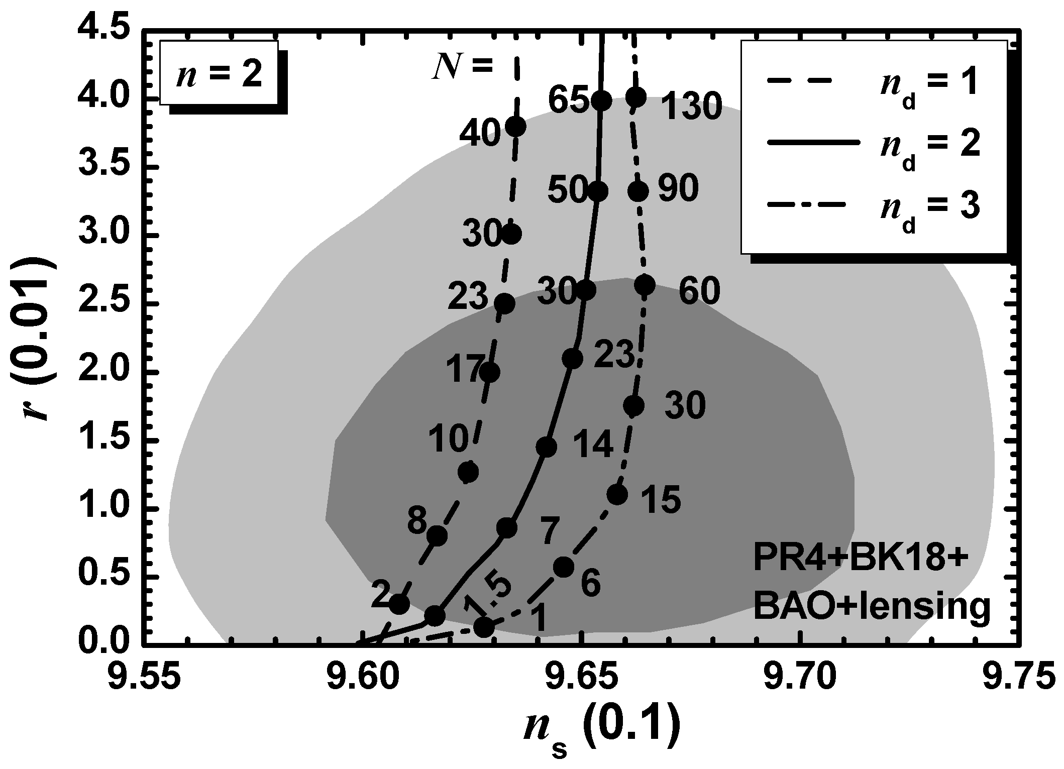
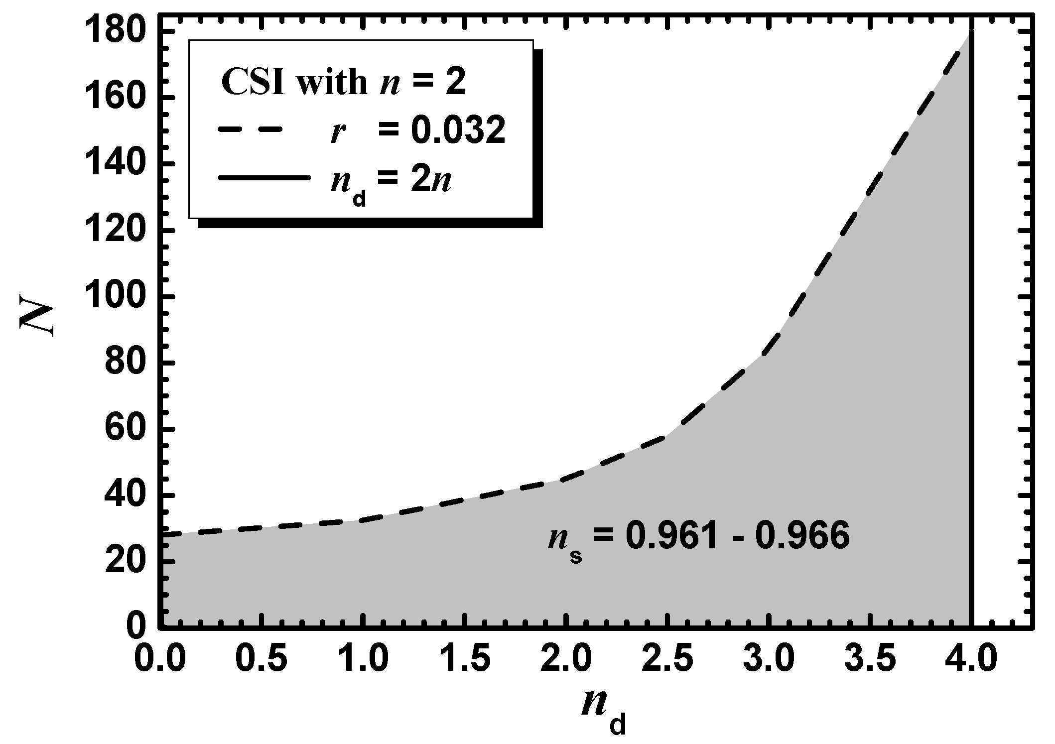
5.2.1. SI with a Gauge-Singlet Inflaton (CSI)

In this case we consider throughout $n=2$ which is motivated by the quadratic potential which is usually encountered for gauge-singlet superfields. The comparison of the model predictions with data is displayed in Figure 1, where we plot r versus $n_{\mathrm{s}}$ for $n_{\mathrm{d}}=1$ (dashed line), $n_{\mathrm{d}}=2$ (solid line) or $n_{\mathrm{d}}=3$ (dot-dashed line). The variation of N is given along each curve. We observe that the whole observationally favored range of r is covered varying N whereas $n_{\mathrm{s}}$ remains close to its central value in Eq. (5.15). As a consequence, an upper bound on N can be derived. This bound increases with $n_{\mathrm{d}}$. Varying continuously N from 1 until that maximal value, derived from the upper bound on r in Eq. (5.15b), we obtain the shaded region in Figure 2. That upper bound, indicated by a dashed line, in conjunction with the upper bound on $n_{\mathrm{d}}$ inferred by Eq. (5.4) and depicted by a solid line, delineate clearly the allowed (shaded) parameter space of our model. In all, we find

$$1\lesssim N\lesssim 180,0\le n_{\mathrm{d}}\le 3.99,0.961\lesssim n_{\mathrm{s}}\lesssim 0.966and1\lesssim {\Delta }_{★}/100\lesssim 53$$

(5.16a)

awith $w_{\mathrm{rh}}\simeq 0$, ${\alpha }_{\mathrm{s}}\simeq -(6.5-7.5)·{10}^{-4}$ and $N_{★}\simeq (50-52)$. It is impressive that the ${\Delta }_{★}$ values are much larger than the values derived in T-model Higgs inflation analyzed in Refs. [54,66,85] and therefore the present model can be characterized as more natural. Note that the naturalness of the model further requests $n_{\mathrm{d}}\ll N$ since in this regime the ’t Hooft argument [69] suits better. Moreover, $\lambda$ and ${\widehat{m}}_{\mathrm{I}}$ range as follows

$$3.6·{10}^{-5}\lesssim \lambda \lesssim 1.4·{10}^{-4}and1.6\lesssim {\widehat{m}}_{\mathrm{I}}/10\mathrm{ZeV}\lesssim 4.7.$$

(5.16b)

The maximal ${\widehat{m}}_{\mathrm{I}}$ values are obtained for the largest $n_{\mathrm{d}}$ and the minimal N – as deduced from the expression shown below Eq. (4.17).

Representative values of model parameters, field values and observables are given in the two leftmost columns of Table 3 for $N=10$. This N value gives $(n_{\mathrm{s}},r)$ in the current “sweet” spot of the dark shaded region in Figure 1. We notice the following: (i) ${\varphi }_{★}$ and ${\varphi }_{\mathrm{f}}$ are subplanckian in accordance with the consideration of SUGRA as an effective theory below $m_{\mathrm{P}}=1$; (ii) ${\Delta }_{★}$ increases with $n_{\mathrm{d}}$; (iii) $\lambda$ acquires a soft dependence from $n_{\mathrm{d}}$ not shown in its analytical expression in Eq. (5.7); (iv) ${\Lambda }_{★}<m_{\mathrm{P}}$ is quite close to $H_{\mathrm{I}★}$ and so the effects of the renormalization-group running are negligible; (v) $w_{\mathrm{rh}}$ estimated by Eq. (5.12) is a little lower than its naive value obtained by Eq. (5.13); (vi) the values derived from the analytical expressions of Section 5.1 and written in italics are quite reliable for $n_{\mathrm{d}}=1$.

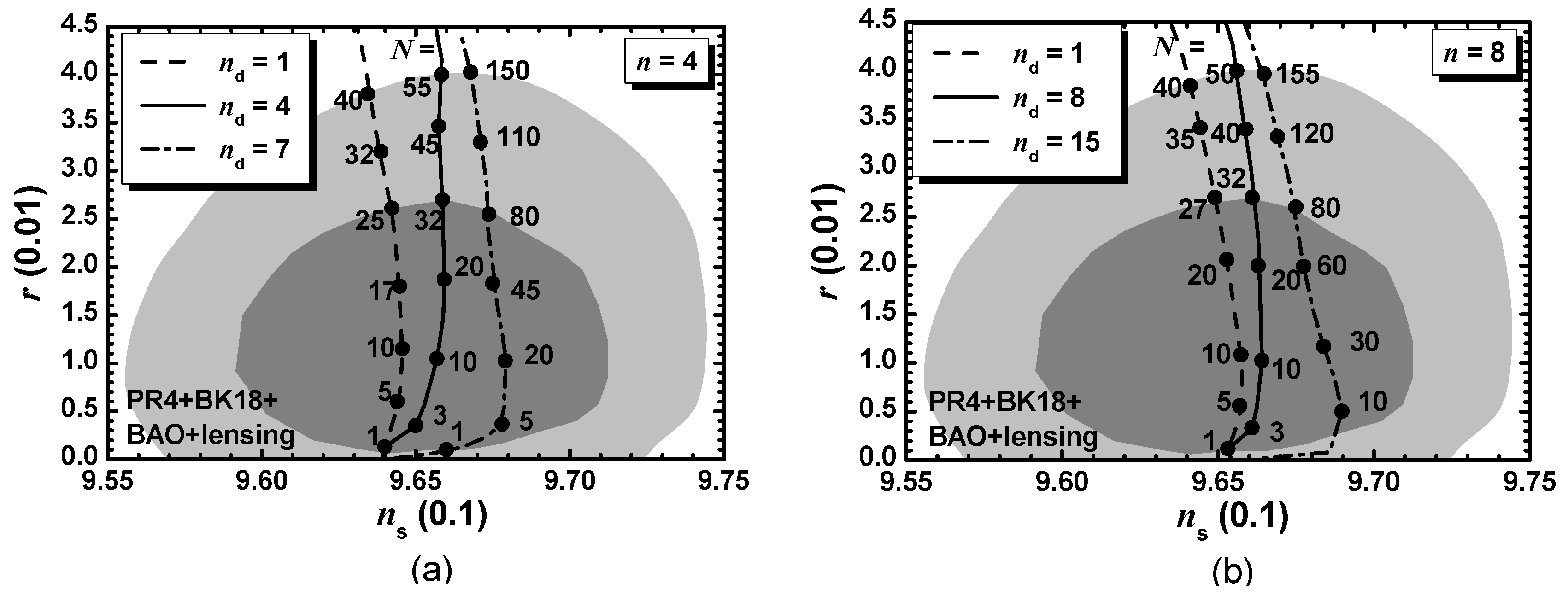
5.2.2. SI with a Higgs Field (HSI)

In this case we consider two representative values, $n=4$ and $n=8$, which are appropriate for the self-consistency of W in Eq. (4.3). We also fix throughout M imposing the GUT condition in Eq. (4.15). Since this is indistinguishable for both K’s considered in Section 4.2, our results are identical for both cases. However, our results are valid for any other M value provided that $M\ll m_{\mathrm{P}}$.

Several characteristic inputs and outputs for HSI with the aforementioned n values are listed in the central and the rightmost columns of Table 3. We take $N=10$ and $n_{\mathrm{d}}=1$ and $n_{\mathrm{d}}=2n-1$ for both selected n values. Recall that viable HSI requires $n_{\mathrm{d}}<2n$ – see Eqs. (5.3) and (5.4). The remarks done in the end of Section 5.2.1 regarding the findings of Table 3 are valid for HSI too. Nonetheless, in this case we present also the M and ${\widehat{m}}_{\mathrm{I}}$ values which are estimated via Eqs. (4.15) and (4.17) correspondingly. We see that both mass parameters decrease as n increases and only ${\widehat{m}}_{\mathrm{I}}$ develops a dependence on $n_{\mathrm{d}}$ as expected from the equations above.

One notable feature of our proposal is the fact that SI takes place for subplanckian $\varphi$ values. The naive assessment that this achievement is not consistent with the chaotic character of SI is not appropriate since $\varphi$ does not coincide with the canonically normalized inflaton, $\widehat{\varphi }$. If we take into account the $\varphi -\widehat{\varphi }$ relation of Eq. (1.2) we can easily infer that $\widehat{\varphi }$ acquires transplackian values for $\varphi <1$ and so SI is rendered feasible – cf. Refs. [10,31,32,33,35,36,54,66]. To clarify further this key feature of our models, we comparatively plot $V_{\mathrm{I}}$ in Eq. (1.3) as a function of $\varphi$ in Figure 3-(a) and $\widehat{\varphi }$ in Figure 3-(b) for $N=10$, $n=4$ and $n_{\mathrm{d}}=1$ (black lines) and $n_{\mathrm{d}}=7$ (gray lines).

From Figure 3-(a) we see that $V_{\mathrm{I}}$ for both $n_{\mathrm{d}}$ values has a parabolic-like slope for $\varphi <1$. On the contrary, in Figure 3-(b) $V_{\mathrm{I}}$ experiences a stretching for $\widehat{\varphi }>1$ which results to the well-known plateau of SI for $\widehat{\varphi }\gg 1$ – see e.g. Ref. [10]. The observationally relevant inflationary period is limited between the two $\varphi$ values ${\varphi }_{\mathrm{f}}$ and ${\varphi }_{★}$ which are given in the two middle columns of Table 3 and are depicted in Figure 3-(a). These values are enhanced, as advocated above, and indicated in Figure 3-(b). Namely, solving Eq. (1.2) w.r.t $\widehat{\varphi }$ we can estimate ${\widehat{\varphi }}_{\mathrm{f}}=2.3$ and ${\widehat{\varphi }}_{*}=9.9$ for $n_{\mathrm{d}}=1$ and ${\widehat{\varphi }}_{\mathrm{f}}=1.5$ and ${\widehat{\varphi }}_{*}=6.8$ for $n_{\mathrm{d}}=7$. In the inset of Figure 3-(a) shown is also the structure of $V_{\mathrm{I}}$ for low $\varphi$ values, responsible for the implementation of the $U{\left(1\right)}_X$ phase transition – see Section 4.4.

From Figure 3b we remark that for both $n_{\mathrm{d}}$ values the magnitudes of the two plateaus are of the order ${10}^{-10}$ which are similar to that obtained in pure SI [10,31,32,36,37,48,49,58]. However, these are one order of lower than that obtained in Ref. [33], where r is a little more enhanced. Indeed, as verified from the values listed in Table 3, the level of the inflationary plateau increases with r. Moreover, the inflationary scale $V_{\mathrm{I}}^{1/4}$ turns out to be well below $m_{\mathrm{P}}$ and so the semi-classical approximation, used in our analysis, is perfectly valid. Note that here $m_{\mathrm{P}}$ is undoubtedly the ultraviolet cut-off scale of the theory thanks to the absence of large coefficients in the K’s. Recall that such large coefficients are used in models of induced-gravity [10,31,32,35,36,37] or non-minimal [48,49] inflation and the aforementioned scale has to be determined after an expansion of $\mathcal{A}$ in Eq. (2.1a) about $\langle \varphi \rangle$.

In order to delineate the available parameter space of HSI for the two selected n values we plot its predictions in the $n_{\mathrm{s}}-r$ plane against the observational data – see Figure 4. To accomplish it, we enforce the constraints in Eq. (5.11) varying N for several $n_{\mathrm{d}}$ values. Namely, for both n values considered, we fix $n_{\mathrm{d}}=1$ (dashed lines), $n_{\mathrm{d}}=n$ (solid lines) or $n_{\mathrm{d}}=2n-1$ (dot-dashed lines). Comparing the structure of these plots with that of Figure 1 we see that this is pretty stable. The $n_{\mathrm{s}}$ values lie close to its central value in Eq. (5.15) with a slight augmentation with $n_{\mathrm{d}}$. The r values increase with N whose the maximum increases with $n_{\mathrm{d}}$. Considering that maximum on N for any allowed $n_{\mathrm{d}}$ we show in Figure 5 for the two considered n values the allowed (shaded) regions in the $n_{\mathrm{d}}-N$ plane. The findings are similar to that in Figure 2 with an decrease of the maximal N’s and an increase of the maximal $n_{\mathrm{d}}$’s depicted by a dashed and a solid line respectively. Obviously, the maximal of the maximal N values are obtained at the intersection of the dashed and the vertical solid lines.

Summarizing our results for $n=4$ – see Figure 5-(a) – we arrive at the following allowed ranges

$$1\lesssim N\lesssim 165,0\le n_{\mathrm{d}}\le 7.99,0.964\lesssim n_{\mathrm{s}}\lesssim 0.968and1\lesssim {\Delta }_{★}/100\lesssim 41$$

(5.17a)

awith $w_{\mathrm{rh}}\simeq 0.3$, ${\alpha }_{\mathrm{s}}\simeq -(5.8-6.5)·{10}^{-4}$ and $N_{★}\simeq (54.-56)$. Moreover, M and ${\widehat{m}}_{\mathrm{I}}$ range as follows

$$3.6\mathrm{YeV}\lesssim M\lesssim 43\mathrm{YeV}and47\mathrm{EeV}\lesssim {\widehat{m}}_{\mathrm{I}}\lesssim 1.8\mathrm{ZeV}.$$

(5.17b)

On the other hand, for $n=8$ – see Figure 5-(b) – we obtain

$$1\lesssim N\lesssim 152,0\le n_{\mathrm{d}}\le 15.99,0.964\lesssim n_{\mathrm{s}}\lesssim 0.969and1\lesssim {\Delta }_{★}/100\lesssim 30$$

(5.18a)

awith $w_{\mathrm{rh}}\simeq 0.5$, ${\alpha }_{\mathrm{s}}\simeq -(5.3-6.2)·{10}^{-4}$ and $N_{★}\simeq (57-59)$. As regards the mass parameters,

$$4.8\mathrm{ZeV}\lesssim M\lesssim 0.17\mathrm{YeV}and0.16\mathrm{PeV}\lesssim {\widehat{m}}_{\mathrm{I}}\lesssim 3.4\mathrm{EeV}.$$

(5.18b)

In both Eqs. (5.17b) and (5.18b) the maximal values are obtained for the lowest N and the largest $n_{\mathrm{d}}$ values whereas the minimal values are achieved at the largest N and the lowest $n_{\mathrm{d}}$ values.

6. Conclusions

We presented a novel implementation of SI (i.e. Starobinsky inflation) in the context of SUGRA confining ourselves to models displaying a kinetic mixing in the inflaton sector with a pole of order two – see Eq. (1.2) – and a scalar potential shown in Eq. (1.3). We considered two classes of models (CSI and HSI) depending on whether the inflaton is included into a gauge singlet or two gauge non-singlet fields. CSI and HSI are relied on the superpotentials in Eqs. (3.3) and (4.3) respectively which respect an R symmetry and include an inflaton-accompanying field which facilitates the establishment of SI. On the other hand, the Kähler potential’s respect the R and gauge symmetries and parameterize hyperbolic internal geometries. Namely, K for CSI is given in Eq. (3.5) whereas for HSI we considered two distinct K’s shown in Eq. (25). The Higgflaton in the last case implements the breaking of a gauge $U{\left(1\right)}_X$ symmetry at a scale which may assume a value compatible with the MSSM unification. All the models excellently match with the observations by restricting the free parameters to reasonably ample regions of values. In particular, the predicted r’s increase with N, while $n_{\mathrm{s}}$ lies close to its central observational value – see Eq. (5.16a) for CSI and Eqs. (5.17a) and (5.18a) for HSI. The present data on ${\delta }_{21}$ and the self-consistency of the models allows us to delineate the overall allowed regions for selected n – see Figure 2 and Figure 5. Hopefully, a more accurate determination of $n_{\mathrm{s}}$ and r by future experiments [94,95,96,97] will assist us to single out the most favorable one from the proposed models.

The central message of our work is that SI is not exclusively implemented by the E-model kinetic mixing in Eq. (1.1). It is also attainable via T-model normalization in Eq. (1.2) if it is considered in conjunction with the potential in Eq. (1.3). The method applied for the construction of our models can be extended to other SUGRA models as those motivated by D branes [98] or those which assist to obtain de Sitter vacua in line with current LHC results on SUSY as in Refs. [57,65]. Moreover, it can employed for supersymmetrizing models obtained adopting the Palatini approach to gravity [99,100,101]. At last, we expect that our models of HSI admit a post-inflationary completion along the lines of Refs. [31,36,37,48,68] since the mass parameters in those models are similar to those found in Eqs. (5.17b) and (5.18b).

Appendix A.1. Shift Symmetry for CSI

We concentrate on the following part of ${\tilde{K}}_{2{\left(11\right)}^2\mathrm{d}}$ in Eq. (3.5)

$${\tilde{K}}_{11}=-Nln{\displaystyle \frac{(1-|\Phi {|}^2)}{{(1-{\Phi }^2)}^{1/2}{(1-{\Phi }^{*2})}^{1/2}}},$$

(A2)

which parameterizes $SU(1,1)/U\left(1\right)$ with curvature ${\mathsf{R}}_{11}=-2/N$. The Kähler metric is a trivial $1\times 1$ matrix with element

$${\mathbf{M}}_{11}={N/(1-|\Phi |}^2{)}^2.$$

(A3)

We then introduce the superfield $\Psi$ via the relation

$$\Phi =tanh{\displaystyle \frac{\Psi }{\sqrt{2N}}}.$$

(A4)

Note that $\Psi$ coincides with canonically normalized inflaton in Eq. (3.8). Inserting it in Eq. (A2), ${\tilde{K}}_{11}$ can be brought into the form

$${\tilde{K}}_{11}=-Nlncosh{\displaystyle \frac{\Psi -{\Psi }^{*}}{\sqrt{2N}}},$$

(A5)

if we take into account the identities of the hyperbolic functions

$$cosh(x-y)=coshxcoshy(1-tanhxtanhy)andcoshx={(1-tanhx)}^{-1/2}.$$

(A6)

From the expression in Eq. (A5), it is clear that ${\tilde{K}}_{11}$ is invariant under the shift symmetry

$$\Psi \to \Psi +cwithc\in \mathbb{R}.$$

(A7)

Therefore, ${\tilde{K}}_{11}$ turns out to be independent from the canonically normalized inflaton, $\widehat{\varphi }$ in Eq. (1.2) which can be identified as the real part of $\Psi$.

Appendix A.2. Shift Symmetry for HSI

We specify the emergence of a shift symmetry in the two K’s used for HSI in Eq. (4.5).

Appendix A.2.1. Kähler  Manifold M (11) 2

We concentrate on the inflationary contribution to ${\tilde{K}}_{2{\left(11\right)}^2\mathrm{d}}$ in Eq. (4.5) which reads

$${\tilde{K}}_{{\left(11\right)}^2}=-{\displaystyle \frac{N}{2}}ln{\displaystyle \frac{{(1-2|\Phi |}^2\left)\right(1-2|\overline{\Phi }{|}^2)}{(1-2\overline{\Phi }\Phi )(1-2{\overline{\Phi }}^{*}{\Phi }^{*})}}$$

(A8)

and parameterizes ${\mathcal{M}}_{{\left(11\right)}^2}={(SU(1,1)/U\left(1\right))}^2$ with curvature ${\mathsf{R}}_{{\left(11\right)}^2}=-4/(N/2)$. The Kähler metric can be represented as a diagonal $2\times 2$ matrix

$${\mathbf{M}}_{{\left(11\right)}^2}=N\mathsf{diag}\left({(1-|\Phi |}^2{)}^{-2},(1-|\overline{\Phi }{{|}^2)}^{-2}\right).$$

(A9)

working along the lines of the previous section, we introduce two superfields $\Psi$ and $\overline{\Psi }$ via the relations

$$\Phi ={\displaystyle \frac{1}{\sqrt{2}}}tanh{\displaystyle \frac{\Psi }{\sqrt{2N}}}and\overline{\Phi }={\displaystyle \frac{1}{\sqrt{2}}}tanh{\displaystyle \frac{\overline{\Psi }}{\sqrt{2N}}}.$$

(A10)

Upon substitution into Eq. (A8), ${\tilde{K}}_{{\left(11\right)}^2}$ can be brought into the form

$${\tilde{K}}_{{\left(11\right)}^2}=-{\displaystyle \frac{N}{2}}ln{\displaystyle \frac{cosh\frac{\Psi -{\Psi }^{*}}{\sqrt{2N}}cosh\frac{\overline{\Psi }-{\overline{\Psi }}^{*}}{\sqrt{2N}}}{cosh\frac{\Psi -\overline{\Psi }}{\sqrt{2N}}cosh\frac{{\overline{\Psi }}^{*}-{\overline{\Psi }}^{*}}{\sqrt{2N}}}}.$$

(A11)

Taking into account that along the inflationary trough in Eq. (4.2) $\Phi =\overline{\Phi }$ and so $\Psi =\overline{\Psi }$, the expression above reduces to the following

$${\left.{\tilde{K}}_{{\left(11\right)}^2}\right|}_{Eq.\left(\right)}=-{\displaystyle \frac{N}{2}}ln{cosh}^2{\displaystyle \frac{\Psi -{\Psi }^{*}}{\sqrt{2N}}}.$$

(A12)

Consequently, $K_{{\left(11\right)}^2}$ is invariant under the shift symmetry of Eq. (A7) and independent from $\mathsf{Re}\Psi =\mathsf{Re}\overline{\Psi }$ i.e. $\widehat{\varphi }$ – see Eqs. (1.2) and (4.11a).

Appendix A.2.2. Kähler  Manifold M 21

Here we focus on the inflationary contribution to ${\tilde{K}}_{221\mathrm{d}}$ in Eq. (4.5) which reads

$${\tilde{K}}_{21}=-Nln{\displaystyle \frac{1-{|\Phi |}^2-{\left|\overline{\Phi }\right|}^2}{{(1-2\overline{\Phi }\Phi )}^{1/2}{(1-2{\overline{\Phi }}^{*}{\Phi }^{*})}^{1/2}}},$$

(A13)

which parameterizes ${\mathcal{M}}_{21}=SU(2,1)/U\left(1\right)$ with curvature ${\mathsf{R}}_{21}=-6/N$. The Kähler metric is a non-diagonal $2\times 2$ matrix

$${\mathbf{M}}_{21}={\displaystyle \frac{N}{F_{\mathrm{T}}^2}}〔\begin{array}{cc}1-|\overline{\Phi }{|}^2& {\Phi }^{*}\overline{\Phi }\\ \Phi {\overline{\Phi }}^{*}& 1-{|\Phi |}^2\end{array}〕,$$

(A14)

where $F_{\mathrm{T}}$ is given in Eq. (4.4). The introduction of the Killing-adapted coordinates can be now performed after diagonalizing ${\mathbf{M}}_{21}$. This can be done via a similarity transformation involving an hermitian matrix $U_{21}$ as follows:

$$U_{21}^{†}{\mathbf{M}}_{21}{U}_{21}=\mathsf{diag}\left({\kappa }_{+},{\kappa }_{-}\right)with{U}_{21}={\displaystyle \frac{1}{\sqrt{{|\Phi |}^2+{\left|\overline{\Phi }\right|}^2}}}〔\begin{array}{cc}|\overline{\Phi }|{\Phi }^{*}/{\overline{\Phi }}^{*}& -|\Phi |\overline{\Phi }/\Phi \\ |\overline{\Phi }|& |\Phi |\end{array}〕.$$

(A15)

The eigenvectors and eigenvalues of ${\mathbf{M}}_{21}$ are given respectively by

$$〔\begin{array}{c}{\dot{\Phi }}_{+}\\ {\dot{\Phi }}_{-}\end{array}〕=U_{21}^{†}〔\begin{array}{c}\dot{\Phi }\\ \dot{\overline{\Phi }}\end{array}〕and\left\{\begin{array}{c}{\kappa }_{+}=N/F_{\mathrm{T}}^2,\hfill \\ {\kappa }_{-}=N/F_{\mathrm{T}}.\hfill \end{array}\right.$$

(A16)

It is very difficult, if not impossible, to integrate the relations above so as to determine generically $\Phi$ and $\overline{\Phi }$ in terms of ${\Phi }_{\pm }$. Therefore we are not able to obtain a generic formula for ${\tilde{K}}_{21}$ as done in Eq. (A11) for ${\tilde{K}}_{{\left(11\right)}^2}$. However, confining ourselves along the direction in Eq. (4.2) and integrating the relevant relations in Eq. (A16) w.r.t the cosmic time we find

$${\Phi }_{+}=(\overline{\Phi }+\Phi )/\sqrt{2}and{\Phi }_{-}=(\overline{\Phi }-\Phi )/\sqrt{2}.$$

(A17)

Solving the system above w.r.t $(\overline{\Phi },\Phi )$ and taking into account that ${\langle {\Phi }_{-}\rangle }_{\mathrm{I}}=0$ – see Eqs. (4.1) and (4.2) – we obtain

$${\left.{\tilde{K}}_{21}\right|}_{Eq.\left(\right)}=-Nln{\displaystyle \frac{1-|{\Phi }_{+}{|}^2}{{(1-{\Phi }_{+}^2)}^{1/2}{(1-{\Phi }_{+}^2)}^{1/2}}}.$$

(A18)

We introduce again a new holomorphic variable ${\Psi }_{+}$ via the relation

$${\Phi }_{+}=tanh{\displaystyle \frac{{\Psi }_{+}}{\sqrt{2N}}}.$$

(A19)

During HSI ${\Psi }_{+}$ becomes the real canonical variable $\widehat{\varphi }$ – see Eqs. (1.2) and (4.11a). Inserting it in Eq. (A18), it can be brought into the form

$${\left.{\tilde{K}}_{21}\right|}_{Eq.\left(\right)}=-Nlncosh{\displaystyle \frac{{\Psi }_{+}-{\Psi }_{+}^{*}}{\sqrt{2N}}}.$$

(A20)

This result manifests the invariance of ${\tilde{K}}_{21}$ under the transformation of Eq. (A7) with $\Psi$ replaced by ${\Psi }_{+}$ and so ${\tilde{K}}_{21}$ is independent from $\mathsf{Re}{\Psi }_{+}=\widehat{\varphi }$ – see Eqs. (4.1) and (A17).

References

1. A.A. Starobinsky, A New Type of Isotropic Cosmological Models Without Singularity, Phys. Lett. B91, 99 (1980).
2. J. Martin, C. Ringeval and V. Vennin, Encyclopædia Inflationaris, Phys. Dark Univ. 5, 75 (2014) [arxiv:1303.3787].
3. J. Martin, C. Ringeval R. Trotta and V. Vennin, The Best Inflationary Models After Planck, 03, no. 14, 039 (2014) [arXiv:1312.3529]. [CrossRef]
4. . Grøn, Predictions of Spectral Parameters by Several Inflationary Universe Models in Light of the Planck Results, Universe 4, no.2, 15 (2018).
5. Y. Akrami et al. [Planck Collaboration], Planck 2018 results. X. Constraints on inflation, Astron. Astrophys.641, A10 (2020) [arxiv:1807.06211].
6. C. Kounnas, D. Lüst and N. Toumbas, R2 inflation from scale invariant supergravity and anomaly free superstrings with fluxes, Fortsch. Phys. 63, 12 (2015) [arxiv:1409.7076]. [CrossRef]
7. M. Galante, R. Kallosh, A. Linde, and D. Roest, Unity of Cosmological Inflation Attractors, Phys. Rev. Lett.114, no. 14, 141302 (2015) [arxiv:1412.3797]. [CrossRef]
8. J. Ellis, D.V. Nanopoulos, K.A. Olive and S. Verner, A general classification of Starobinsky-like inflationary avatars of SU(2,1)/SU(2)×U(1) no-scale supergravity, J. High Energy Phys. 03, 099 (2019) [arxiv:1812.02192]. [CrossRef]
9. J. Ellis, M.A.G. Garcia, N. Nagata, D.V. Nanopoulos, K.A. Olive and S. Verner, Building Models of Inflation in No-Scale Supergravity, Int. J. Mod. Phys. D 29, 16, 2030011 (2020) [arxiv:2009.01709]. [CrossRef]
10. C. Pallis and N. Toumbas, Starobinsky Inflation: From Non-SUSY To SUGRA Realizations, Adv. High Energy Phys.2017, 6759267 (2017) [arxiv:1612.09202]. [CrossRef]
11. See, e.g., P. Binétruy, Supersymmetry: Theory, experiment and cosmology, Oxford (2006).
12. S. Navas et al. [Particle Data Group], Review of particle physics, Phys. Rev. D110, no.3, 030001 (2024).
13. F. Wang, W. Wang, J. Yang, Y. Zhang and B. Zhu, Low Energy Supersymmetry Confronted with Current Experiments: An Overview, Universe 8, no. 3, 178 (2022) [arxiv:2201.00156].
14. W. Buchmuller, V. Domcke and K. Kamada, The Starobinsky Model from Superconformal D-Term Inflation, Phys. Lett. B 726, 467 (2013) [arxiv:1306.3471]. [CrossRef]
15. S. Basilakos, N.E. Mavromatos and J. Sola, Starobinsky-like inflation and running vacuum in the context of Supergravity, Universe 2, no. 3, 14 (2016) [arxiv:1505.04434]. [CrossRef]
16. S.V. Ketov and A. A. Starobinsky, Embedding (R+R2)-Inflation into Supergravity, Phys. Rev. D 83, 063512 (2011) [arxiv:1011.0240].
17. R. Blumenhagen, A. Font, M. Fuchs, D. Herschmann and E. Plauschinn, Towards axionic Starobinsky-like inflation in string theory, Phys. Lett. B746, 217 (2015) [arxiv:1503.01607]. [CrossRef]
18. T. Li, Z. Li and D.V. Nanopoulos, Helical phase in ation via non-geometric flux compactifications: from natural to Starobinsky-like inflation, J. High Energy Phys. 10, 138 (2015) [arxiv:1507.04687].
19. J. Ellis, D.V. Nanopoulos and K.A. Olive, No-Scale Supergravity Realization of the Starobinsky Model of Inflation, Phys. Rev. Lett. 111, 111301 (2013) – Erratum: Phys. Rev. Lett. 111, no. 12, 129902 (2013) [arxiv:1305.1247].
20. J. Ellis D. Nanopoulos and K. Olive, Starobinsky-like Inflationary Models as Avatars of No-Scale Supergravity, 10, 009 (2013) [arXiv:1307.3537].
21. J. Ellis, H.-J. He and Z.-Z. Xianyu, New Higgs inflation in a no-scale supersymmetric SU(5) GUT, Phys. Rev. D 91 021302 (2015) [arxiv:1411.5537]. [CrossRef]
22. I. Garg and S. Mohanty, No-scale SUGRA SO(10) derived Starobinsky model of inflation, Phys. Lett. B 751, 7 (2015) [arxiv:1504.07725]. [CrossRef]
23. J. Ellis, M.A.G. Garcia, N. Nagata, D.V. Nanopoulos and K.A. Olive, Starobinsky-like Inflation, Supercosmology and Neutrino Masses in No-Scale Flipped SU(5), 07, 006 (2017) [arxiv:1704.07331].
24. J. Ellis, M.A.G. Garcia, N. Nagata, D.V. Nanopoulos and K.A. Olive, Starobinsky-Like Inflation and Neutrino Masses in a No-Scale SO(10) Model, 11, 018 (2016) [arXiv:1609.05849].
25. E. Cremmer, S. Ferrara, C. Kounnas and D.V. Nanopoulos, Naturally Vanishing Cosmological Constant in N=1 Supergravity, Phys. Lett. B133, 61 (1983); [CrossRef]
26. A.B. Lahanas and D.V. Nanopoulos, The Road to No-Scale Supergravity, Phys. Rept.145, 198 (1987). [CrossRef]
27. S. Cecotti, Higher Derivative Supergravity Is Equivalent To Standard Supergravity Coupled To Matter, Phys. Lett. B 190, 86 (1987). [CrossRef]
28. F. Farakos, A. Kehagias and A. Riotto, On the Starobinsky Model of Inflation from Supergravity, Nucl. Phys. B876, 187 (2013) [arxiv:1307.1137].
29. R. Kallosh and A. Linde, Superconformal generalizations of the Starobinsky model, 062013028 [arxiv:1306.3214].
30. A.B. Lahanas and K. Tamvakis, Inflation in no-scale supergravity, Phys. Rev. D91, 085001 (2015) [arxiv:1501.06547].
31. C. Pallis, Linking Starobinsky-Type Inflation in no-Scale Supergravity to MSSM, 042014024; 07, 01(E) (2017) [arxiv:1312.3623].
32. C. Pallis, Induced-Gravity Inflation in no-Scale Supergravity and Beyond, 057 (2014) [arXiv:1403.5486].
33. C. Pallis, Reconciling induced-gravity inflation in supergravity with the Planck 2013 & BICEP2 results, 10, 058 (2014) [arXiv:1407.8522]. [CrossRef]
34. R. Kallosh, More on Universal Superconformal Attractors, Phys. Rev. D89, no. 8, 087703 (2014) [arxiv: 1402.3286]. [CrossRef]
35. C. Pallis and N. Toumbas, Starobinsky-Type Inflation With Products of Kähler Manifolds, 05, no. 05, 015 (2016) [arXiv:1512.05657]. [CrossRef]
36. C. Pallis and Q. Shafi, Induced-Gravity GUT-Scale Higgs Inflation in Supergravity, Eur. Phys. J. C78, no.6, 523 (2018) [arxiv:1803.00349].
37. C. Pallis, Starobinsky-Type B-L Higgs Inflation Leading Beyond MSSM, PoS CORFU2022, 101 (2023) [arxiv:2305.00523].
38. R. Kallosh, A. Linde and T. Rube, General inflaton potentials in supergravity, Phys. Rev. D83, 043507 (2011) [arxiv:1011.5945]. [CrossRef]
39. H.M. Lee, Chaotic inflation in Jordan frame supergravity, 08, 003 (2010) [arXiv:1005.2735]. [CrossRef]
40. I. Antoniadis, E. Dudas, S. Ferrara and A. Sagnotti, The Volkov – Akulov – Starobinsky Supergravity, Phys. Lett. B 733, 32 (2014) [arxiv:1403.3269].
41. Y. Aldabergenov, Volkov–Akulov–Starobinsky supergravity revisited, Eur. Phys. J. C 80, no. 4, 329 (2020) [arxiv:2001.06617].
42. S. Ferrara, R. Kallosh and A. Linde, Cosmology with Nilpotent Superfields, J. High Energy Phys. 10, 2014 (143) [arxiv:1408.4096]. [CrossRef]
43. I. Antoniadis, D.V. Nanopoulos and K.A. Olive, R2–Inflation Derived from 4d Strings, the Role of the Dilaton, and Turning the Swampland into a Mirage, arxiv:2410.16541.
44. A. Zee, A Broken Symmetric Theory of Gravity, Phys. Rev. Lett.42, 417 (1979). [CrossRef]
45. G.F. Giudice and H.M. Lee, Starobinsky-like inflation from induced gravity, Phys. Lett. B733, 58 (2014) [arxiv:1402.2129]. [CrossRef]
46. C. Pallis and Q. Shafi, Non-minimal chaotic inflation, Peccei-Quinn phase transition and non-thermal leptogenesis, Phys. Rev. D 86, 023523 (2012) [arxiv:1204.0252].
47. C. Pallis and Q. Shafi, Gravity Waves From Non-Minimal Quadratic Inflation, 03, 023 (2015) [arxiv:1412.3757]. [CrossRef]
48. C. Pallis, Unitarity-Safe Models of Non-Minimal Inflation in Supergravity, Eur. Phys. J. C 78, no.12, 1014 (2018) [arxiv:1807.01154]. [CrossRef]
49. C. Pallis, Unitarizing non-Minimal Inflation via a Linear Contribution to the Frame Function, Phys. Lett. B789, 243 (2019) [arXiv:1809.10667]. [CrossRef]
50. A. Kehagias, A.M. Dizgah and A. Riotto, Remarks on the Starobinsky model of in ation and its descendants, Phys. Rev. D 89, 043527 (2014) [arxiv:1312.1155].
51. T. Terada, Generalized Pole Inflation: Hilltop, Natural, and Chaotic Inflationary Attractors, Phys. Lett. B760, 674 (2016) [arxiv:1602.07867].
52. B.J. Broy, M. Galante, D. Roest and A. Westphal, Pole inflation, Shift symmetry and universal corrections, J. High Energy Phys. 12, 149 (2015) [arxiv:1507.02277]. [CrossRef]
53. T. Kobayashi, O. Seto and T.H. Tatsuishi, Toward pole inflation and attractors in supergravity : Chiral matter field inflation, Prog. Theor. Phys. 123B04, no.12 (2017) [arxiv:1703.09960]. [CrossRef]
54. C. Pallis, Pole Inflation in Supergravity, PoS CORFU 2021, 078 (2022) [arXiv:2208.11757].
55. S. Karamitsos and A. Strumia, Pole inflation from non-minimal coupling to gravity, J. High Energy Phys. 05, 016 (2022) [arxiv:2109.10367]. [CrossRef]
56. J.J.M. Carrasco, R. Kallosh, A. Linde and D. Roest, Hyperbolic geometry of cosmological attractors, Phys. Rev. D92, no. 4, 041301 (2015) [arxiv:1504.05557].
57. J.J.M. Carrasco, R. Kallosh and A. Linde, α-Attractors: Planck, LHC and Dark Energy, J. High Energy Phys. 10, 147 (2015) [arxiv:1506.01708].
58. C. Pallis, An Alternative Framework for E-Model Inflation in Supergravity, Eur. Phys. J. C 82, no. 5, 444 (2022) [arxiv:2204.01047]. [CrossRef]
59. R. Kallosh, A. Linde, and D. Roest, Superconformal Inflationary a-Attractors, J. High Energy Phys. 11, 198 (2013) [arxiv:1311.0472]. [CrossRef]
60. R. Kallosh and A. Linde, Universality Class in Conformal Inflation, 07, 002 (2013) [arxiv:1306.5220].
61. R. Kallosh and A. Linde, BICEP/Keck and cosmological attractors, 12, no.12, 008 (2021) [arXiv:2110.10902]. [CrossRef]
62. J. Ellis, M.A.G. Garcia, D.V. Nanopoulos, K.A. Olive and S. Verner, BICEP/Keck constraints on attractor models of inflation and reheating, Phys. Rev. D 105, no. 4, 043504 (2022) [arxiv:2112.04466]. [CrossRef]
63. S. Bhattacharya, K. Dutta, M.R. Gangopadhyay and A. Maharana, α-attractor inflation: Models and predictions, Phys. Rev. D107, no. 10, 103530 (2023) [arxiv:2212.13363].
64. K. Dimopoulos, Introduction to Cosmic Inflation and Dark Energy, CRC Press, ISBN 978-0-367-61104-0 (2020).
65. J. Ellis, D. V. Nanopoulos, K. A. Olive and S. Verner, Unified No-Scale Attractors, 09, 040 (2019) [arXiv:1906.10176]. [CrossRef]
66. C. Pallis, Pole-induced Higgs inflation with hyperbolic Kähler geometries, 05, 043 (2021) [arXiv:2103.05534]. [CrossRef]
67. C. Pallis, SU(2,1)/(SU(2)×U(1)) B-L Higgs Inflation, J. Phys. Conf. Ser.2105, no. 12, 12 (2021) [arxiv:2109.06618].
68. C. Pallis, T-Model Higgs Inflation in Supergravity, arXiv:2307.14652.
69. G. ’t Hooft, Naturalness, chiral symmetry, and spontaneous chiral symmetry breaking, NATO Sci. Ser. B59, 135 (1980).
70. M. Kawasaki, M. Yamaguchi and T. Yanagida, Natural chaotic inflation in supergravity, Phys. Rev. Lett. 85, 3572 (2000) [hep-ph/0004243]. [CrossRef]
71. P. Brax and J. Martin, Shift symmetry and inflation in supergravity, Phys. Rev. D 72, 023518 (2005) [hep-ph/0504168]. [CrossRef]
72. S. Antusch, K. Dutta and P.M. Kostka, SUGRA Hybrid Inflation with Shift Symmetry, Phys. Lett. B 677, 221 (2009) [arxiv:0902.2934].
73. T. Li, Z. Li and D.V. Nanopoulos, Supergravity Inflation with Broken Shift Symmetry and Large Tensor-to-Scalar Ratio, 02, 028 (2014) [arXiv:1311.6770].
74. C. Pallis, Kinetically modified nonminimal chaotic inflation, Phys. Rev. D91, 123508 (2015) [arxiv: 1503.05887].
75. C. Pallis, Kinetically Modified Non-Minimal Inflation With Exponential Frame Function, Eur. Phys. J. C 77, no. 9, 633 (2017) [arxiv:1611.07010]. [CrossRef]
76. I. Ben-Dayan and M.B. Einhorn, Supergravity Higgs Inflation and Shift Symmetry in Electroweak Theory, 12, 002 (2010) [arXiv:1009.2276]. [CrossRef]
77. G. Lazarides and C. Pallis, Shift Symmetry and Higgs Inflation in Supergravity with Observable Gravitational Waves, J. High Energy Phys. 11, 114 (2015) [arxiv:1508.06682]. [CrossRef]
78. C. Pallis, Kinetically modified nonminimal Higgs inflation in supergravity, Phys. Rev. D92, no. 12, 121305 (2015) [arxiv:1511.01456].
79. C. Pallis, Variants of Kinetically Modified Non-Minimal Higgs Inflation in Supergravity, 10, 037 (2016) [arXiv:1606.09607].
80. R. Kallosh, A. Linde, D. Roest and T. Wrase, Sneutrino inflation with α-attractors, 11, 046 (2016) [arXiv:1607.08854].
81. T.E. Gonzalo, L. Heurtier and A. Moursy, Sneutrino driven GUT Inflation in Supergravity, J. High Energy Phys. 06, 109 (2017) [arxiv:1609.09396]. [CrossRef]
82. K. Kaneta, Y. Mambrini, K. A. Olive and S. Verner, Inflation and Leptogenesis in High-Scale Supersymmetry, Phys. Rev. D101, no.1, 015002 (2020) [arxiv:1911.02463]. [CrossRef]
83. J. Ellis, M.A.G. Garcia, D.V. Nanopoulos and K.A. Olive, Phenomenological aspects of no-scale inflation models, 10, 003 (2015) [arxiv:1503.08867]. [CrossRef]
84. Y. Ema, M.A. G. Garcia, W. Ke, K.A. Olive and S. Verner, Inflaton Decay in No-Scale Supergravity and Starobinsky-like Models, Universe 10, no. 6, 239 (2024) [arxiv:2404.14545]. [CrossRef]
85. C. Pallis, T-Model Higgs Inflation and Metastable Cosmic Strings, J. High Energy Phys. 01, ?? (2025) [arxiv:2409.14338].
86. C. Pallis, E- and T-model hybrid inflation, Eur. Phys. J. C 83, no. 1, 2 (2023) [arxiv:2209.09682]. [CrossRef]
87. N. Aghanim et al. [Planck Collaboration], Planck 2018 results. VI. Cosmological parameters, Astron. Astrophys.641, A6 (2020) – Erratum: Astron. Astrophys.652, C4 (2021) [arxiv:1807.06209].
88. M.S. Turner, Coherent Scalar-Field Oscillations in an Expanding Universe Phys. Rev. D 28, 1243 (1983).
89. J. Martin and C. Ringeval, First CMB Constraints on the Inflationary Reheating Temperature, Phys. Rev. D 82, 023511 (2010) [arxiv:1004.5525]. [CrossRef]
90. J. Ellis, M.A.G. Garcia, D.V. Nanopoulos and K.A. Olive, Calculations of Inflaton Decays and Reheating: with Applications to No-Scale Inflation Models, 07, 050 (2015) [arxiv:1505.06986]. [CrossRef]
91. C.M. Lin, On the oscillations of the inflaton field of the simplest α-attractor T-model, Chin. J. Phys. 86, 323 (2023) [arxiv:2303.13008].
92. M. Tristram et al., Improved limits on the tensor-to-scalar ratio using BICEP and Planck, Phys. Rev. Lett. 127, 151301 (2021) [arxiv:2112.07961].
93. P.A.R. Ade et al. [BICEP and Keck Collaboration], Improved Constraints on Primordial Gravitational Waves using Planck, WMAP, and BICEP/Keck Observations through the 2018 Observing Season, Phys. Rev. Lett.127, no. 15, 151301 (2021) [arxiv:2110.00483].
94. K. Abazajian et al., CMB-S4 Science Case, Reference Design, and Project Plan, arxiv:1907.04473.
95. P. Andre et al. [PRISM Collaboration], PRISM (Polarized Radiation Imaging and Spectroscopy Mission): A White Paper on the Ultimate Polarimetric Spectro-Imaging of the Microwave and Far-Infrared Sky, arxiv:1306.2259.
96. L. Montier et al. [LiteBIRD Collaboration], Overview of the Medium and High Frequency Telescopes of the LiteBIRD satellite mission, Proc. SPIE Int. Soc. Opt. Eng. 11443, 114432G (2020) [arxiv:2102.00809].
97. D. Baumann et al. [CMBPol Study Team Collaboration], CMBPol Mission Concept Study: Probing Inflation with CMB Polarization, AIP Conf. Proc.1141, 10 (2009) [arxiv:0811.3919].
98. R. Kallosh and A. Linde, Polynomial α-attractors, 04, no. 04, 2022 (017) [arXiv:2202.06492].
99. F. Bauer and D.A. Demir, Higgs-Palatini Inflation and Unitarity, Phys. Lett. B698, 425 (2011) [arxiv: 1012.2900]. [CrossRef]
100. V.M. Enckell, K. Enqvist, S. Rasanen and L.P. Wahlman, Inflation with R2 term in the Palatini formalism, Phys. Lett. B02, 022 (2019) [arxiv:1810.05536].
101. I. Antoniadis, A. Karam, A. Lykkas and K. Tamvakis, Palatini inflation in models with an R2 term, Phys. Lett. B11, 028 (2018) [arxiv:1810.10418].
Figure 1. Curves allowed by Eq. (5.11) in the n s r plane for CSI with n = 2 , various N’s indicated along them and n d = 1 (dashed line), n d = 2 (solid line) or n d = 3 (dot-dashed line). The marginalized joint 68 % [ 95 % ] c.l. regions [92] from PR4, BK18, BAO and lensing data-sets are depicted by the dark [light] shaded contours.
Preprints 148113 g001
Figure 2. Allowed (shaded) region as determined by Eqs. (5.11) and (5.15) in the n d N plane for CSI with n = 2 . The conventions adopted for the boundary curves are also shown.
Preprints 148113 g002
Figure 3. Inflationary potential V I as a function of (a) ϕ and (b) ϕ ^ fixing M X = M GUT . We consider HSI with N = 10 , n = 4 and n d = 1 (black lines) or n d = 7 (gray lines). Values corresponding to ϕ and ϕ f (a) or ϕ ^ and ϕ ^ f (b) are depicted. Shown is also the low- ϕ behavior of V I in the inset (a).
Preprints 148113 g003
Figure 4. Curves allowed by Eq. (5.11) in the n s r plane for HSI with M X = M GUT and various N’s indicated along them. We take (a) n = 4 and n d = 1 (dashed line), n d = 4 (solid line) or n d = 7 (dot-dashed line) or (b) n = 8 and n d = 1 (dashed line), n d = 8 (solid line) or n d = 15 (dot-dashed line). The shaded regions are identified as in Figure 1.
Preprints 148113 g004
Figure 5. Allowed (shaded) region as determined by Eqs. (5.11) and (5.15) in the n d N plane for HSI with M X = M GUT and (a) n = 4 or (b) n = 8 . The conventions adopted for the boundary lines are also shown.
Preprints 148113 g005