Submitted:
04 February 2025
Posted:
04 February 2025
You are already at the latest version
Abstract
This paper introduces a novel bioelectromechanical device converting the electrochemical potential energy of excitable cells into mechanical work by coupling the Hodgkin–Huxley (HH) neuronal model response to a mechanical resonator. Addressing key challenges in bioelectromechanical systems, including biocompatibility, miniaturization, and efficient energy conversion, the device leverages the membrane potentials of biological cells to drive mechanical oscillations within microelectromechanical systems (MEMS). Through a combination of numerical simulations and theoretical analyses, it is demonstrated that the coupled HH–resonator system achieves stable limit cycles and significant mechanical displacements via parametric amplification. This amplification arises from the nonlinear capacitive coupling, which leads to Mathieu-like equations governing the system’s dynamics, thereby enabling large oscillations from relatively small voltage inputs. Such parametric resonance is critical for the device's ability to sustain oscillatory motion, making it highly suitable for integration into compact and implantable MEMS applications. Potential applications include implantable sensors and actuators for real-time physiological monitoring, and advanced micro-scale systems that benefit from biologically sourced energy. The findings underscore the promise of bioelectromechanical systems in advancing biomedical and microengineering technologies, paving the way for innovative solutions in personalized medicine, bio-robotics, and beyond.
Keywords:
bioelectromechanical systems
; Hodgkin–Huxley model
; parametric resonance
; microelectromechanical systems (MEMS)
; nonlinear capacitive coupling
; electrostatic actuation
; action potential
; energy conversion
; biocompatible actuators
; bio-hybrid microsystems
1. Introduction
The development of bioelectromechanical devices capable of converting electrochemical potential energy from biological cells into mechanical energy represents a significant advancement in the field of bioengineering. This research aims to address the challenges associated with the miniaturization and optimization of such devices, focusing on their potential applications in medicine, bioengineering, and microelectromechanical systems (MEMS).
MEMS have emerged as a pivotal technology in biomedical applications, offering the potential to revolutionize medical diagnostics, therapeutics, and monitoring [1]. These systems integrate mechanical elements, sensors, actuators, and electronics on a common silicon substrate, enabling the creation of devices with high functionality and small size. Advancements in MEMS have led to the development of implantable devices such as micropumps, biosensors, and micro-robots, which are designed to offer better diagnostic and therapeutic methods [2,6,7].
A comprehensive review [3] highlights the significant advancements in MEMS for biomedical applications, emphasizing their role in diagnostics, therapeutics, and monitoring. The authors discuss the integration of MEMS with biological systems, noting that such integration has led to the development of devices capable of precise and early detection of medical conditions, as well as therapeutic interventions.
Despite these advancements, several challenges persist in the miniaturization and optimization of bioelectromechanical devices. One major obstacle is the development of flexible and biocompatible materials that can withstand the physiological environment without causing adverse reactions. Efforts have been made to address this by focusing on polymer processing to develop flexible implantable devices with high biocompatibility [4,5].
Another significant challenge is the efficient conversion of electrochemical energy from biological cells into mechanical energy [8]. Traditional methods often face limitations due to the complexity of biological systems and the need for precise control over energy conversion processes. The intricate nature of biological systems introduces challenges in accurately controlling energy conversion processes. For instance, the storage of energy in ATP was first detected in anaerobic energy-yielding reactions but soon was also found in respiratory and photosynthetic energy production. However, the mechanism by which energy derived from metabolites was converted into phosphate-bond energy in these processes appeared to be complex and not fully understood [9].
Furthermore, the Second Law of thermodynamics implies that no thermodynamic system with a single heat source at constant temperature can convert heat into mechanical work in a recurrent manner [10].
Recent research has explored various approaches to overcome these limitations, including the development of microresonators coupled to excitable cells to induce periodic oscillations, thereby converting electrochemical energy into mechanical energy [11].
These complexities highlight the need for innovative approaches to achieve efficient and controlled energy conversion in biological systems.
The proposed bioelectromechanical device aims to address the challenges identified in the current state of the art by utilizing the membrane potential and action potential activation of excitable cells to drive an electromechanical circuit. This approach offers several advantages:
- Efficient Energy Conversion: By directly harnessing the electrochemical potential of biological cells, the device achieves more efficient energy conversion compared to traditional methods.
- Biocompatibility and Miniaturization: Utilizing biological cells as the energy source ensures compatibility with the human body, reducing the risk of adverse reactions. Additionally, the device's design allows for significant miniaturization, making it suitable for applications where space and invasiveness are critical concerns.
- Flexible Architectural Design: The mechanical oscillator, realized through electrostatic actuation, can be easily scaled and adapted to multiple configurations. Increasing the number of capacitor plates or excitable cells proportionally boosts the actuation force and available power. This modularity supports diverse applications such as micropumps, micropropellers for drug delivery, and other micromechanical subsystems.
Potential applications of this technology include: i) implantable sensors and actuators powered by the device could monitor and respond to physiological conditions in real-time, offering new avenues for personalized medicine. ii) the device could be integrated into prosthetics and assistive devices, providing a sustainable power source that adapts to the user's biological systems. iii) The device's compact size and efficient energy conversion make it ideal for integration into MEMS, enabling the development of advanced micro-scale systems with enhanced capabilities.
In summary, this research seeks to advance the field of bioelectromechanical systems by developing a device that effectively converts electrochemical energy from biological cells into mechanical energy, addressing current challenges and opening new possibilities in medicine, bioengineering, and MEMS applications.
2. Structural Design of the Proposed Bio-Electromechanical Device
The primary goal of the proposed bio-electromechanical device is to utilize the membrane potential, specifically the action potential activation of at least one excitable cell, to power an electromechanical circuit. This circuit comprises at least one resistor, one capacitor, and a mechanical oscillator, where the oscillator is mechanically coupled to the mobile plate of the capacitor.
The device is designed to harness the electrochemical potential energy generated by the differential concentrations of ion species inside and outside the cellular membrane. This energy is then converted into mechanical energy through a system consisting of at least one excitable cell and an electromechanical microresonator. The microresonator cyclically excites the action potential of the cell, thereby inducing periodic oscillations. These oscillations form a self-sustaining system capable of generating mechanical energy for practical applications.
As illustrated in Figure 1, the proposed device is characterized by its compact dimensions, ranging approximately from 10 to 200 microns, with an optimal operational range between 20 and 100 microns. The electrical parameters include maximum voltages around 100 mV, currents in the nanoampere range, and associated power levels on the order of 10−10 W. Coupling between the electromechanical microresonator and the cell body is achieved through at least one resistor and, optionally, additional impedance components. The mechanical oscillator is integrally fixed to the mobile plate of the capacitor, while the opposing plate remains stationary, facilitating the desired energy conversion process.
The device is organized into two primary coupled circuits: the driving circuit and the electromechanical converting circuit, each serving distinct roles in the energy conversion process.
The driving circuit (labeled as Circuit 1 in Figure 1) includes at least one excitable cell, such as a neuron or similar biological cell capable of generating action potentials. The cell membrane acts as the central element, electrically connected through terminals and to both internal and external cellular regions. These terminals are coupled to a current generator and an impedance . The current plays a critical role in modulating the membrane current to ensure efficient triggering of the action potential.
The electromechanical converting circuit (labeled as Circuit 2 in Figure 1) is primarily passive and consists of two main parts: the electrical and mechanical subsystems.
- Electrical Subsystem: The core electrical component is a capacitor () with a capacitance , connected in parallel to the current generator. An additional impedance may be incorporated to optimize performance in specific configurations.
- Mechanical Subsystem: The mechanical component is represented by an elastic mechanical oscillator, which can be realized in various configurations. In the simplest model, the oscillator consists of a mass , an elastic element with stiffness , and a dissipative element characterized by a damping coefficient . The mobile plate of the capacitor is mechanically coupled to the oscillator, enabling the conversion of electrostatic forces into mechanical oscillations.
The operation of the device hinges on the precise design of the external current , which must fall within an optimal range to maintain system functionality. If is too small, the membrane current is insufficient to trigger action potentials. Conversely, if is too large, the excessive current induces rapid refractory states in the cell, inhibiting periodic oscillations.
When is within the optimal range, the driving circuit generates periodic current spikes. These spikes induce a cyclic potential difference across terminals and , leading to the periodic charging and discharging of the capacitor . The resulting electrostatic forces between the capacitor plates drive the oscillations of the mechanical oscillator, thereby producing the desired biomotor effect.
The system's functionality is defined by its ability to convert the electrochemical energy of the excitable membrane into mechanical energy. This process activates a limit cycle within the bio-electromechanical system, resulting in self-sustaining oscillations. The mechanical energy generated can be directly applied to power microdevices, offering a scalable and efficient solution for various applications.
The key features of the proposed device are: i) the compact size, ranging from 10 to 200 microns, facilitating integration into microscale systems. ii) Efficient Energy Conversion, directly harnesses electrochemical potential from biological cells, enhancing conversion efficiency. Iii) Biocompatibility, utilizing biological cells as an energy source, ensuring compatibility with physiological environments. Iv) Scalable Design: Modular architecture allows for the addition of multiple capacitor plates or excitable cells, proportionally increasing actuation force and power output. Iv) Versatile Applications: Suitable for implantable sensors, actuators, prosthetics, and advanced MEMS-integrated micro-scale systems.
By addressing the challenges of miniaturization, biocompatibility, and efficient energy conversion, the proposed bio-electromechanical device represents a step forward in the development of bio-hybrid microsystems with diverse biomedical and engineering applications.
3. Mathematical Modeling of the Bio-Electromechanical Device
3.1. General Introduction to the Hodgkin-Huxley Model
The electrical behavior of the excitable membrane is described using the HH model [12], which provides a robust quantitative foundation for understanding the membrane’s dynamic properties. This section details the mathematical representation of the system, emphasizing its nonlinear differential equations, the membrane's ionic dynamics, and their role in generating a periodic driving force for the electromechanical components.
The power contributions in the Hodgkin-Huxley (HH) model can be categorized into distinct components that reflect the energy transformations occurring within the neuronal membrane. These components account for external stimulation, capacitive storage, ionic dissipation, and the influence of electromotive forces. Below is a detailed description of each term.
The excitable membrane, represented in Figure 2, is modeled as a capacitor () with a dielectric formed by the lipid bilayer. This bilayer is combined with selective ionic channels that regulate ion flow based on voltage differentials. For this study, the focus is on sodium () and potassium () ions, which play essential roles in generating and propagating action potentials; in this model the leakage channel is not considered.
The sodium and potassium channels are characterized as variable resistors ( and ), each in series with constant voltage generators to reflect their voltage-dependent behavior. Hodgkin and Huxley demonstrated that the conductances of these channels ( and ) dynamically depend on the transmembrane potential (). During an action potential, the conductances increase significantly, reducing the channel resistances and facilitating ion flow. This decrease in resistance highlights the membrane's changing permeability in response to the electric field and provides clear evidence that the action potential is driven by variations in ionic fluxes across the membrane. The resistances are expressed as and , where the conductances depend on both time and membrane potential.
Unlike the ionic channels, which can be modeled as resistors and respond to a step current input with a corresponding step change in voltage, the neuronal membrane exhibits a continuous voltage response under similar conditions. This distinction arises because the membrane behaves as a capacitor, where altering the potential across it requires modifying the charge stored on its plates. In the neuronal membrane, this process is analogous to redistributing charge across its interfaces through ionic fluxes, which drive depolarization.
The relationship between the voltage across a capacitor and the charge stored on its plates is given by: where represents the charge, and is the capacitance, serving as the proportionality constant between and . The change in charge, and consequently the voltage across the capacitor, is induced by current flow. Current is defined as the rate of charge transfer over time: Substituting this into the capacitor equation yields: From this relationship, it becomes clear that the voltage change across the capacitor in response to a current pulse is directly proportional to the duration of the current. This continuous variation of membrane potential highlights the capacitor-like behavior of the neuronal membrane in contrast to the step responses of purely resistive ionic channels.
In series with these resistors are ionic batteries ( and ), which represent the electromotive forces arising from ionic concentration gradients.
In the HH model, ionic currents are modeled as flow through variable resistances in parallel with a capacitor that represents the membrane. For each ion considered (e.g., sodium and potassium), the current depends on the difference between the membrane potential and the ion's equilibrium potential, which is determined by the Nernst equation. The total current flowing through the membrane () is thus the sum of the capacitive current and the ionic currents.
The capacitive current () is related to the rate of change of the membrane potential () over time. Since the membrane is represented as a capacitor, the capacitive current is given by: where is the membrane capacitance per unit area.
The ionic currents () are driven by the conductances of the sodium and potassium channels ( and ), which depend on both time and the membrane potential, reflecting the voltage-dependent nature of the channels. For sodium and potassium ions, the currents are expressed as: where and are the equilibrium potentials, respectively. These potentials represent the voltages at which there is no net ionic flow for the corresponding ion species.
The total membrane current is given by: which, for the case of two ion species, can be expanded as: equation:
This formulation captures the dynamic interplay between the capacitive and ionic components of the current, as well as their dependence on the time-varying membrane potential. It provides the foundation for analyzing how the membrane potential evolves during processes like the action potential, where rapid changes in ion channel conductances lead to characteristic voltage fluctuations.
Hodgkin and Huxley developed equations to describe the time-dependent conductances of ion channels, ensuring they remained sufficiently simple for computing action potentials and refractory periods. A significant challenge in modeling these conductances lay in their distinct behaviors during depolarization and repolarization. Specifically, sodium () and potassium () conductances increase with a delay during depolarization and decrease rapidly during repolarization.
Using experimental data obtained via the patch-clamp technique, Hodgkin and Huxley demonstrated that sodium conductance is proportional to the third power of an activation variable, , governed by a first-order differential equation, with an additional term accounting for the progressive inactivation of sodium channels, . Similarly, potassium conductance is proportional to the fourth power of its activation variable, , also governed by a first-order differential equation. These relationships are expressed as:
,
here, and represent the maximum attainable values of sodium and potassium conductances, respectively, while , , and are dimensionless gating variables that range between 0 and 1, that indicate the likelihood of the corresponding ion channel being open, allowing ions to move between the intracellular and extracellular fluids. Their values depend on both membrane voltage and time, reflecting the dynamic nature of channel gating. Their dynamics are governed by the following first-order differential equations:
The rate constants and are voltage-dependent and describe the transition rates of ion channels between open and closed states. Let denote a general gating variable, such as , , or . The dynamics of can be described by:
where is the equilibrium fraction of open channels, and is the relaxation time. These equations highlight the following key points:
- Individual ion channel proteins transition stochastically between open and closed states.
- The fraction of open channels, , relaxes exponentially toward , the equilibrium value.
- The relaxation rate to equilibrium is determined by the time constant .
The voltage-dependence of and , as determined by Hodgkin and Huxley's experiments, leads to exponential dependencies of reaction rates on membrane voltage (see Table 1).
Consequently, the equilibrium fraction and time constant exhibit sigmoidal dependencies on voltage, reflecting the nonlinear reaction kinetics of ion channel gating. This interplay between voltage and gating dynamics forms the foundation for understanding the behavior of excitable membranes and their role in action potential generation.
Indicating with the index for (sodium) or (potassium), the Nernst potentials () and maximum conductances () are provided in the Table 2. The term accounts for different resting potentials commonly adopted in various studies, which are typically either or . In this work, is taken to be .
At equilibrium, the cell maintains a resting potential, primarily governed by the efflux of ions through weakly active potassium channels. Sodium channels are largely inactive at this state. Disturbances in the membrane potential, if sufficient in magnitude, initiate the activation of sodium channels, leading to a sequence of ionic exchanges that constitutes the action potential.
The dynamics of the membrane are captured by the following system of nonlinear differential equations, derived from the HH model:
Here:
- : Membrane capacitance [].
- : Transmembrane potential [.
- : Maximum conductances of sodium and potassium channels [].
- , : Nernst potentials [] for sodium and potassium, respectively.
- , represent the activation and inactivation variables for sodium channels, respectively, while n represents the activation variable for potassium channels.
- , , : Steady-state activation and inactivation functions (voltage-dependent).
- , , : Voltage-dependent time constants.
- : External current per unit area applied across the membrane [].
The first equation in system (1) represents the balance of currents across the cell membrane, as illustrated in Figure 2. This equation accounts for the combined contributions of ionic currents and external current inputs. The remaining three equations describe the dynamics of the ionic channels, specifically the constitutive relationships governing the variable resistances depicted in the diagram in Figure 2.
3.2. Power Balance in the Hodgkin-Huxley Model
The power contributions in the HH model can be categorized into distinct components that reflect the energy transformations occurring within the neuronal membrane. These components account for external stimulation, capacitive storage, ionic dissipation, and the influence of electromotive forces. Below is a detailed description of each term.
The external power is provided by the applied current and is responsible for driving the system. The instantaneous power supplied by is given by:
The external power can drive changes in the capacitive charge, sustain ionic currents, or both. In Figure 5, is represented in the third subplot from the top.
The power associated with the membrane's capacitive charging or discharging is:
This term reflects the rate at which electrical energy is stored or released from the capacitive component of the membrane. In Figure 5, is shown in the second subplot from the top and indicated with The power dissipated by the ionic currents is given by:
where and are the power dissipation rates for sodium and potassium channels, respectively. For each ionic channel:
These terms represent the resistive dissipation of energy due to ion flow through voltage-dependent channels. In Figure 4, and are displayed in the first subplot.
The HH model includes voltage sources representing the Nernst potentials ( and ) for sodium and potassium ions, respectively. These potentials contribute additional power, defined as:
where and are the ionic currents through the sodium and potassium channels: These terms quantify the work done by the ion-specific electromotive forces in driving ionic currents. Unlike , these contributions do not result in heat dissipation but are essential for maintaining ionic gradients and facilitating proper neural function. In Figure 5, and are also represented in the first subplot.
The power balance of the HH model is described by the following relationship:
indicating that the power supplied externally is distributed among three components: energy storage in the membrane capacitance, dissipative losses through ionic channels and energy exchange facilitated by the Nernst potentials.
3.3. Numerical Simulations of the Hodgkin-Huxley Model
Numerical simulations are performed with the values listed in Table 1 and Table 2. Initial condition of Eq. 1 are and The external current is used as regulation parameter.
The way the HH model processes external current to generate action potentials is fundamental, as this conversion of synaptic input into action potentials forms the cornerstone of neuronal communication and brain functionality. When a low-level external current is applied, ionic fluctuations occur until the system stabilizes at a new steady state characterized by slightly elevated membrane potentials. With moderate external current input, the membrane potential may briefly exceed the action potential threshold, producing a single spike before returning to a steady state. Biologically, this reflects ion redistribution in response to changes in electrostatic pressure.
Figure 3 illustrates the neuronal response to , a steady stream of action potentials is generated. The HH model not only attributes action potential generation to ionic current changes but also faithfully captures the timing and voltage characteristics of these events, ensuring biologically accurate simulations.
Figure 3 further demonstrates how ionic conductance changes correspond to the various phases of an action potential. At the onset of an action potential, the conductance of Na+ () rapidly increases due to the activation of -gates, enabling a substantial influx of Na+ ions. This inward current amplifies depolarization through a positive feedback loop, driving the rapid upstroke of the action potential. At the peak, however, begins to decrease due to the inactivation of Na+ channels via the -gates, thereby limiting further Na+ entry. Sodium ions subsequently leave the cell, driven by electrochemical gradients, as the channels close.
In contrast, potassium conductance () increases more gradually as -gates slowly activate. This delayed efflux of K+ ions counteracts the depolarizing effects of Na+ influx and ultimately dominates during the repolarization phase. The delayed activation of -gates ensures a robust repolarization process, restoring the membrane potential toward its resting state. The persistence of elevated after repolarization results in an after-hyperpolarization, a transient state where the membrane potential becomes more negative than the resting level. This state is critical for resetting the neuronal membrane and ensuring unidirectional action potential propagation.
The interplay between Na+ channel inactivation (-gates closing) and K+ channel activation (-gates opening) creates a refractory period during which further action potential initiation is inhibited. This separation of successive spikes prevents excessive neuronal firing and ensures orderly signal transmission.
The voltage- and time-dependent behavior of the gating variables , , and allows the HH model to accurately capture the biophysical mechanisms underlying action potentials. The distinct time constants and voltage sensitivities of the gating variables contribute to the characteristic waveform of action potentials and their critical role in neural signaling.
Figure 4 illustrates the Fourier transformation of the signal, highlighting a dominant frequency slightly below 70 Hz. This result is consistent with the temporal periodicity observed in Figure 3, where the signal exhibits a period of approximately 0.015 seconds.
With the aid of Figure 5 and Figure 6 it is possible to understand the power fluxes within the membrane. Specifically, to facilitate the visualization of power exchanges, the first subplot of Figure 6 displays the combined power contributions from the individual ionic channels ( and ) along with the capacitive power (). These components are related to the external power (), represented in the second subplot.
Figure 4.
FFT of the signal .
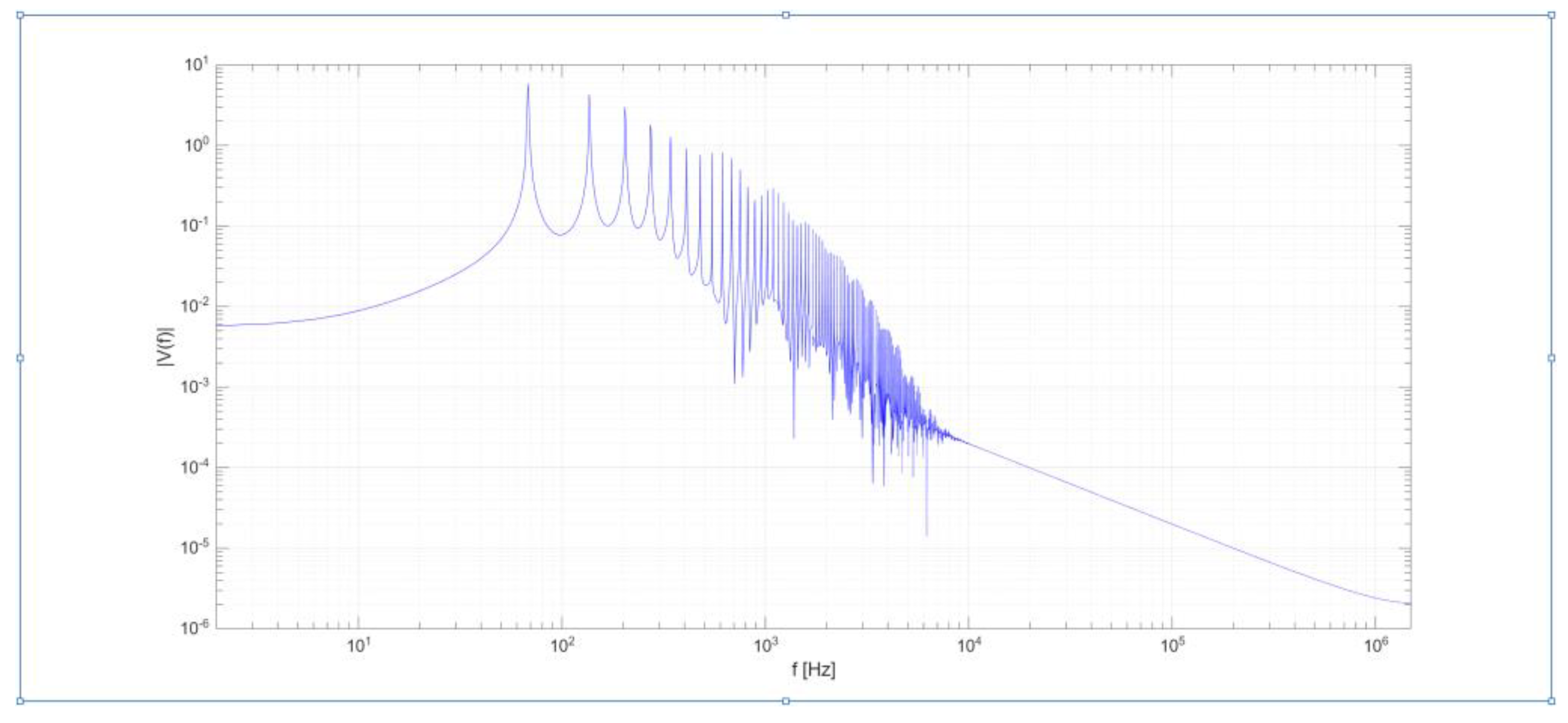
Figure 5.
The figure displays the power components of a single charge-discharge cycle organized into three subplots due to differing -axis scales: (top) ionic power contributions (, , , ); (middle) capacitive power (); (bottom) external power ().
Figure 5.
The figure displays the power components of a single charge-discharge cycle organized into three subplots due to differing -axis scales: (top) ionic power contributions (, , , ); (middle) capacitive power (); (bottom) external power ().
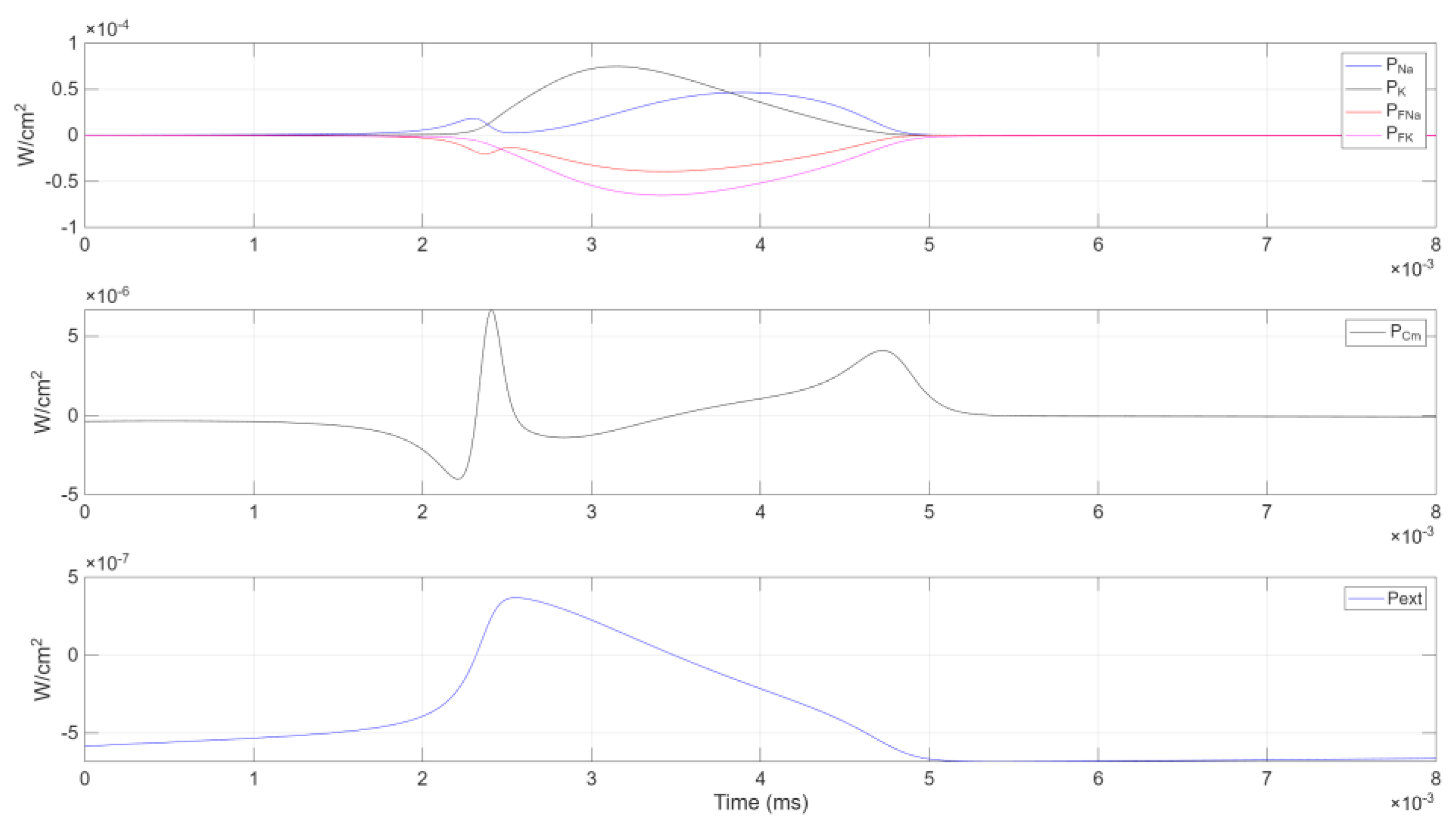
Figure 6.
The first subplot shows the combined power contributions from the ionic channels ( and ) and the capacitive power (). The second subplot illustrates the external power ().
Figure 6.
The first subplot shows the combined power contributions from the ionic channels ( and ) and the capacitive power (). The second subplot illustrates the external power ().
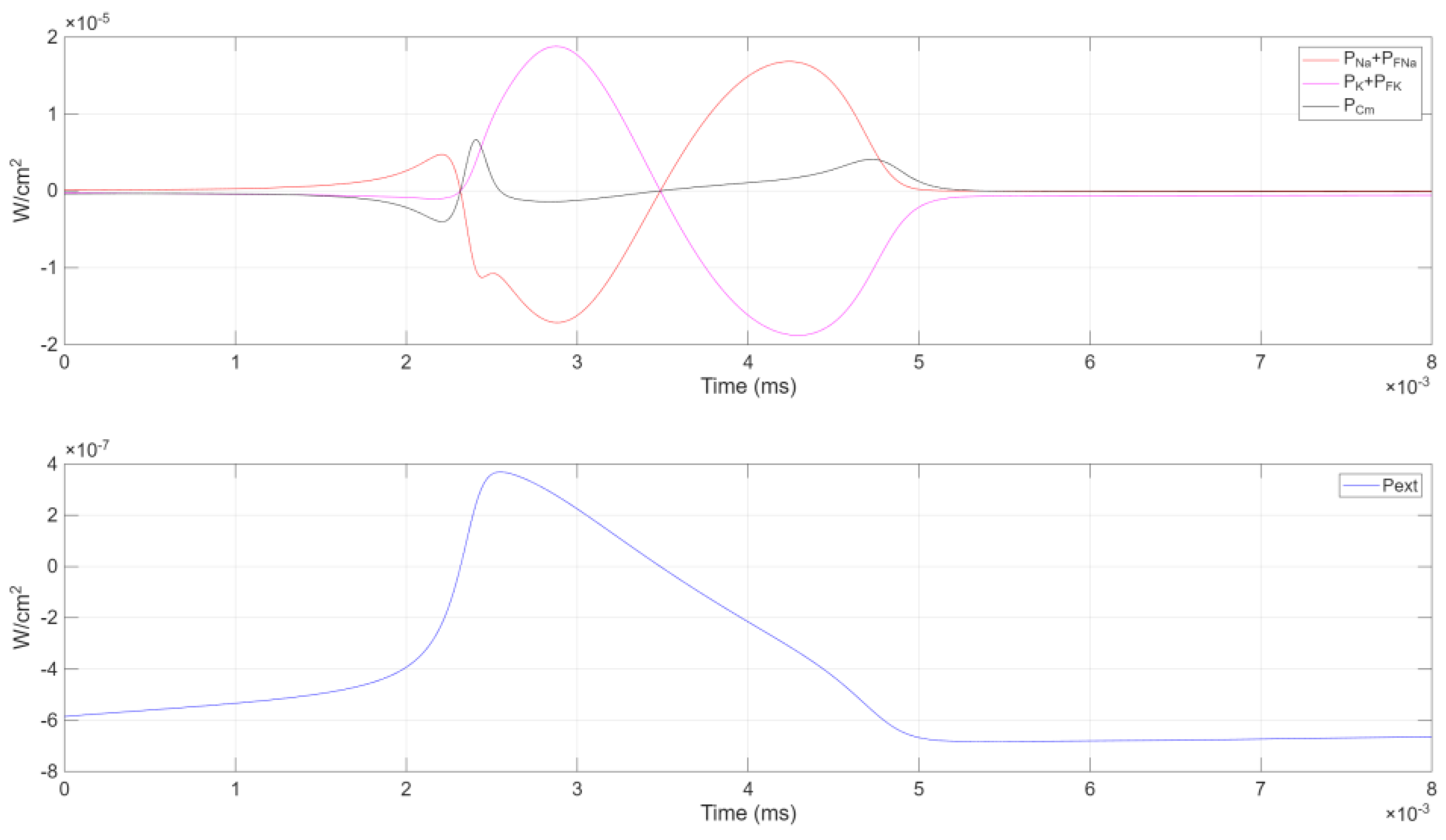
Figure 6 reveals the interdependent temporal evolution of , , and the combined ionic channel powers and :
- Initial Phase. transitions from negative values to zero, reflecting a diminishing energy supply from the external current. It then peaks positively around . Meanwhile, —the power in the membrane capacitance —shows a complementary response: dropping to a negative extremum, then surging to a positive peak shortly thereafter.
- Sodium Channel Power. The combined sodium channel power closely mirrors but with opposite polarity. It peaks positively at —when is at its minimum—and then decreases to a local minimum at . Shortly after the external power peak, it reaches an absolute minimum at .
- Potassium Channel Power. The total potassium channel power lags behind the sodium channel, exhibiting an opposite trend. When rises, drops, and vice versa. Its positive peak emerges slightly delayed, in line with potassium’s role in repolarization.
- Convergence and Next Cycle. Notably, at , all internal power terms converge to zero, while remains positive and continues to decrease. Soon after, becomes positive and becomes negative, with both reaching extreme values at . A subsequent relative maximum in appears at . Finally, dips into negative territory, completing one cycle of power exchange and preparing the system for the next.
This analysis underscores the cyclical energy flow within the HH framework. Depolarization involves strong coupling between capacitive charging and sodium ion flux, while repolarization is facilitated by potassium’s delayed conductance. After hyperpolarization, the system transitions to a state where the external current again becomes the primary energy source, allowing the cycle to repeat.
These power exchanges emphasize both the electrical storage and dissipation mechanisms inherent in neuronal activity. The external energy supply sustains the rapid influx and efflux of ions through voltage-gated channels, restoring the membrane potential after each depolarization event. Through this lens, the Hodgkin–Huxley model not only captures the electrophysiological behavior of excitable cells but also provides a framework for analyzing the energetics and metabolic costs of neuronal signaling.
3.4. Integration of the Hodgkin-Huxley Model with a Elettro-Mechanical Oscillator
The coupling of the HH neuronal model with a electro-mechanical oscillator introduces a novel bioelectromechanical system, enabling the direct conversion of membrane potentials into mechanical motion. This integration leverages the dynamic properties of the HH model and incorporates the capacitive behavior of the membrane into a resonating mechanical structure. The system’s equations are presented below in coherence with the notation used in this study.
Focusing on the analysis of the driving circuit (1) with the electromechanical converting circuit (2), as illustrated in Figure 1, the complete system integrates the neuronal membrane described by the HH model with a mechanical resonator. This resonator comprises a mass (M), a spring with stiffness (K), and a damping element characterized by the coefficient (D). Additionally, the mechanical oscillator is equipped with a capacitor, whose capacitance varies with the displacement of the oscillator’s movable plate.
To ensure the compatibility of the two systems, the HH model equations (1) —formulated in terms of specific quantities such as current per unit area—are scaled by the total membrane area , in this case, a cell radius of 5000was assumed. The membrane dynamics are governed by the following set of equations:
Here is the current in capacitor coupled to the elastic mechanical oscillator.
The mechanical oscillator is described by the following second-order differential equation:
where:
- is the displacement of the movable plate of the capacitor,
- is the surface area of the capacitor plates,
- is the displacement-dependent capacitance of the capacitor, is the permittivity of free space,
- represents the rest distance between the fixed and movable plates of the capacitor incorporated into the resonator, it ensures the capacitor has a finite capacitance in its rest state.
The term on the right-hand side of the equation represents the electrostatic force exerted by the capacitor, which depends on the square of the transmembrane potential and the displacement-dependent capacitance.
Note that to integrate this equation with the HH model, which utilizes time in milliseconds, we redefine the time variable as (ms): This substitution affects the time derivatives as follows: Substituting these into the mechanical oscillator equation yields:
where: is time in milliseconds (ms), remains in meters (m), , , and retain their SI units (kg, N·s/m, and N/m respectively). This normalization ensures that the time scales of the mechanical oscillator are directly compatible with those of the HH neuronal model, facilitating coherent integration of the bioelectrical and mechanical dynamics.
When the HH model is integrated with the mechanical oscillator, the membrane potential influences the resonator’s motion through the variable capacitor, and the displacement x in turn modifies the capacitance seen by the membrane. This two-way feedback links the bioelectrical and mechanical components and can produce complex dynamical behavior. Rewriting eq.s (2) and (3) in a normal form:
the last equation can also be written as where: and Energy Considerations
The powers associated with the electro-mechanical resonator in the coupled HH and resonator system are derived from the mechanical energy components and their interactions with the capacitor.
The variable capacitor depends on the resonator’s displacement x(t), the instantaneous energy stored in this capacitor is: . Consequently, the instantaneous power associated with Ca arises from the time derivative of this electrostatic energy: . After substitution with the actual value of , the formula produces:
The first term quantifies the power contribution due to the mechanical motion of the capacitor plate, while the second term, corresponds to the conventional power exchange from changes in the voltage across the capacitor at a given capacitance.
Power due to the resonator's kinetic energy, to the spring force and dissipated by the resonator's damping are listed below:
The total power balance for the resonator alone is:
When the resonator is coupled with the HH model, the complete power balance reads:
recalling that the previously calculated powers for the HH model, in section 3.2, were specific powers, they must be multiplied by the cell surface area to obtain the total power contributions.
The energy exchanges in the coupled system can be categorized into: i) Electrochemical Energy, represented by the ionic currents and the capacitive charging/discharging of the membrane; ii) Mechanical Energy: comprising kinetic energy, potential energy, and dissipation; iii) Electrostatic Energy, stored in the capacitor of the mechanical oscillator.
4. Numerical Simulations and Discussion
Numerical simulations are performed with the values listed in Table 1 and Table 2. Initial condition of Eq. 1 are and initial condition for the displacement and velocity of the oscillator are null.
The external current is set . For a spherical cell, is calculated as: where is the cell radius. Assuming , the cell surface area is: The physical parameters of the oscillator are set as follows. Figure 3 and 4 indicate that the fundamental period of the ensuing oscillatory process is about . To achieve sufficiently large oscillation amplitude in the mechanical oscillator, its natural frequency should be tuned to match that of the driving circuit, namely: Thus, selecting: follows In a similar fashion, let the viscous damping factor , it follows ; the other parameters are Figure 7 shows the membrane potential, along with the displacement and velocity of the mechanical oscillator, plotted versus time. While the time behaviour of the membrane potential remains nearly identical to that of the uncoupled scenario, the oscillator exhibits a characteristic oscillatory behaviour consisting of an initial transient phase followed by a steady-state regime. During the initial transient, a harmonic amplitude modulation emerges: its carrier frequency is approximately , whereas the modulating frequency is considerably lower and roughly matches the difference between the driving frequency and the system’s natural frequency.
The frequency content of these responses are illustrated in Figure 8, which displays the normalized Fourier transform, ensuring a consistent scale across all spectra. From Figure 8, one can observe that the oscillator’s displacement predominantly concentrates its energy at , chosen to be close to the driving frequency. Additionally, there is a less energetic peak at lower frequency, roughly 10 Hz, which accounts for the low-frequency oscillation associated with the amplitude-modulated (AM) wave. This low-frequency component decays after a characteristic time span.
The typical timescale of the transient vibration is given by , beyond three times this interval, the transient behaviour subsides, and the oscillator settles into stable vibrations around a mean displacement of slightly less than 10−6 m. The duration and prominence of the initial AM wave are governed by the damping factor ζ. Altering ζ leads to distinct changes in both the amplitude and frequency of the observed modulation, thereby influencing the overall transient dynamics of the coupled system.
Figure 9 presents the energy contributions associated with both the neuronal membrane and the mechanical resonator. The first two subplots exhibit behavior closely resembling that of the uncoupled HH model, in Figure 5. Examination of the resonator reveals that, given the small displacements and velocities involved, the primary energetic contribution arises from the capacitor. This contribution can be separated into a mechanical term, stemming from the variation in capacitance, and an electrical term, resulting from the voltage changes across the capacitor over time.
It has been noted that the external current can serve as a control parameter. Figure 10 illustrates the behavior of the coupled system when this external current is set to 3 μA. After a single cycle, the membrane potential settles into a stable value, effectively inhibiting further pulsatile behavior. Likewise, following the initial transient phase, the resonator’s displacement converges to a fixed position, and its velocity becomes zero, indicating that the mechanical subsystem also reaches a steady equilibrium. In conclusion, by exploiting this mechanism in a cyclic manner, it becomes possible to induce periodic action potential firing in the driving circuit, effectively establishing a limit cycle in the bioelectric system. An opposing regulatory mechanism counters the effect of the external current by returning the membrane potential toward equilibrium. Consequently, when the external current again drives the membrane away from this equilibrium, another spike is generated, producing a stable, repeating sequence of action potentials. Notably, this spiking behaviour—and thus the resulting limit cycle—only emerges for suitable values of .
In the proposed work, the mechanical oscillator uses a simple electrostatic actuator composed of a single capacitor with two facing plates. Where required by specific applications, multiple pairs of plates can be incorporated—common in electrostatic microactuator technology—to proportionally increase both the actuation force and the resulting displacement. The same principle applies to the number of neuronal cells included in the bio-motor: employing multiple excitable cells or cell bodies, for example in an electrically connected ensemble, proportionally augments the power delivered to the mechanical oscillator.
Furthermore, the mechanical oscillator can serve as an actuator element in any micromechanical device, thus functioning as the principal motor. A promising application of this bio-electromechanical system is in micropump technology. In this setup, the mobile capacitor plate acts as the movable wall of a variable-volume chamber. Two one-way valves are typically installed in the chamber, ensuring that as the membrane oscillates, it generates a pulsatile fluid flow. This mechanism can be exploited to pump biological fluids or other liquids in a controlled, cyclic manner.
5. Theoretical Analysis of Parametric Amplification in Coupled Hodgkin–Huxley and Mechanical Oscillator Systems
This chapter illustrates how the nonlinear dependence of the capacitance on the resonator’s displacement can induce parametric resonance, ultimately amplifying the mechanical oscillations. By combining a first-order Taylor expansion of the position-dependent capacitance with a dominant harmonic representation of the driving voltage, the system’s governing equation takes a Mathieu-like form [13], highlighting the conditions under which small oscillations grow significantly.
Consider the dynamic equation of the mechanical oscillator coupled with HH model:
where ; represents the electrostatic force generated by a capacitor charged to a voltage .
For small oscillations, expand about :
where
Higher-order terms (e.g., ) are omitted to keep the analysis tractable. Suppose the driving voltage is dominated by a single harmonic:
In practice, additional DC or higher-frequency components may be incorporated; however, the principal mechanism of interest arises from the primary harmonic1.
Substituting the Taylor-expanded and the single-harmonic voltage gives:
Expanding and simplifying using the identity :
Neglecting higher-order terms () for small oscillations, the force simplifies to:
Substituting the expanded electrostatic force back into the oscillator’s equation of motion:
rearranges to:
Dividing through by and defining and , the equation becomes:
This resembles the standard Mathieu equation:
where encapsulates the modulation strength proportional to , and the damping term has been disregarded.
If the modulation frequency is near the system’s natural frequency , small disturbances in can be amplified substantially. The damping limits unbounded growth, but moderate damping still allows significantly larger amplitudes compared to ordinary (single-frequency) forced resonance.
In summary, by modeling the capacitor’s displacement dependence to first order and approximating the voltage with its dominant harmonic, the system’s governing equation naturally displays parametric resonance features. This leads to the well-known Mathieu-like behavior, where the mechanical oscillator’s amplitude can be substantially amplified at or near the resonant frequency. In the context of a coupled Hodgkin–Huxley and electro-mechanical oscillator framework, these results offer insights into how bioelectrical signals, once rectified and fed into a nonlinear electrostatic actuator, may yield significant mechanical outputs through parametric amplification.
This simplified derivation underscores the power of nonlinear coupling in electromechanical systems, highlighting both the potential for large amplitude oscillations and the need to carefully consider damping, frequency tuning, and operating conditions to harness or mitigate parametric effects in practical devices. In MEMS or bioelectromechanical devices, this effect can be harnessed to obtain large displacements from relatively small voltage inputs, provided the operating frequency and damping are suitably tuned.
6. Conclusions
This work has introduced a bioelectromechanical system that couples the Hodgkin–Huxley (HH) neuronal model with a mechanical resonator, demonstrating how electrochemical potential energy can be harnessed to produce mechanical work. Numerical simulations reveal that, within specific parameter ranges, the membrane potential achieves a stable limit cycle characterized by periodic action potentials, subsequently driving small yet significant displacements in the resonator. The external current and mechanical parameters (e.g., damping, stiffness) emerge as decisive control variables for inducing or suppressing sustained oscillations.
From a theoretical standpoint, modelling the capacitor’s displacement dependence to first order and approximating the voltage with its dominant harmonic naturally leads to parametric resonance. In such a framework, the system’s governing equation adopts Mathieu-like characteristics, where small perturbations can be substantially amplified at or near the resonant frequency. In the context of a coupled HH and mechanical oscillator system, these findings clarify how bioelectrical signals, once rectified and directed into a nonlinear electrostatic actuator, may yield significant mechanical outputs through parametric amplification.
This simplified derivation underscores the power of nonlinear coupling in electromechanical devices, highlighting both the potential for large-amplitude oscillations and the necessity of carefully balancing damping, frequency tuning, and operating conditions. In micromechanical or bioelectromechanical technologies—such as micropumps or implantable actuators—this effect can be leveraged to achieve considerable displacements from relatively small voltage inputs.
Future studies will focus on refining this theoretical insight by investigating higher-order nonlinearities, long-term stability, biocompatible materials, and broader ranges of biological cell networks, ultimately broadening the functionality and practical applications of such bio-hybrid systems.
Author Contributions
Conceptualization, A. Carcaterra and N. Roveri; methodology, A. Carcaterra and N. Roveri; software, S. Milana and G. Pepe; validation, S. Milana and G. Pepe; formal analysis, A. Carcaterra and N. Roveri; data curation, A. Carcaterra and N. Roveri; writing —original draft preparation, N. Roveri.; writing—review and editing, N. Roveri and S. Milana; supervision, A. Carcaterra. All authors have read and agreed to the published version of the manuscript.
Funding
This research received no external funding.
Data Availability Statement
No new data was created.
Acknowledgments
In this section, you can acknowledge any support given which is not covered by the author contribution or funding sections. This may include administrative and technical support, or donations in kind (e.g., materials used for experiments).
Conflicts of Interest
The authors declare no conflicts of interest.
Abbreviations
The following abbreviations are used in this manuscript:
- HH:Hodgkin–Huxley
- MEMS:Microelectromechanical Systems
- :External current
- :Membrane capacitance
- :Variable capacitor (capacitor associated with the resonator)
- :Sodium ionic current
- :Potassium ionic current
- :Nernst potential for sodium
- :Nernst potential for potassium
- :Capacitive power (energy stored/released by the membrane capacitor)
- :Ionic dissipation power
- and :Electromotive power contributions (Nernst) for sodium and potassium, respectively
- :External power
- :Impedance in the driving circuit
- :Additional impedance in the electromechanical converting circuit
- :Elastic constant (stiffness) of the mechanical oscillator
- :Mass of the mechanical oscillator
- :Damping coefficient of the mechanical oscillator
- :Angular frequency of the input signal (voltage)
- :Natural frequency of the mechanical oscillator
- :Damping ratio
| 1 | In practice, the voltage V(t) within the HH model exhibits a periodic temporal behavior composed of multiple harmonics—approximately five in Figure 4—spanning an order of magnitude in frequency. While these higher harmonics contribute to the overall waveform, the principal mechanism of parametric amplification arises from the primary harmonic. Consequently, the Mathieu equation remains a valid approximation for capturing the core dynamics of the system. However, the presence of additional harmonics may introduce minor perturbations, potentially requiring more sophisticated analytical techniques for a comprehensive description. For the purposes of this analysis, the single-harmonic approximation sufficiently captures the essential parametric amplification behavior observed numerically. |
References
- Nayem Hossain, Md Zobair Al Mahmud, Amran Hossain, Md Khaledur Rahman, Md Saiful Islam, Rumana Tasnim, Md Hosne Mobarak, Advances of materials science in MEMS applications: A review, Results in Engineering, Volume 22, 2024, 102115, ISSN 2590-1230. [CrossRef]
- 2. Zhang D, Gorochowski TE, Marucci L, Lee HT, Gil B, Li B, Hauert S, Yeatman E. Advanced medical micro-robotics for early diagnosis and therapeutic interventions. Front Robot AI. 2023 Jan 10;9:1086043. [CrossRef]
- ”Chircov, C.; Grumezescu, A.M. Microelectromechanical Systems (MEMS) for Biomedical Applications. Micromachines 2022, 13, 164. [CrossRef]
- ”Pavlov, V.A., Tracey, K.J. Bioelectronic medicine: updates, challenges and paths forward. Bioelectron Med 5, 1 (2019). https://doi.org/10.1186/s42234-019-0018-y.
- ”Dinis, H., and P. M. Mendes. "A comprehensive review of powering methods used in state-of-the-art miniaturized implantable electronic devices." Biosensors and Bioelectronics 172 (2021): 112781..
- ”Ji, B.; Gao, K. Editorial for the Special Issue on Wearable and Implantable Bio-MEMS Devices and Applications. Micromachines 2024, 15, 955. [CrossRef]
- ”Çağlayan, Z.; Demircan Yalçın, Y.; Külah, H. A Prominent Cell Manipulation Technique in BioMEMS: Dielectrophoresis. Micromachines 2020, 11, 990. [CrossRef]
- ”Lueke, J.; Moussa, W.A. MEMS-Based Power Generation Techniques for Implantable Biosensing Applications. Sensors 2011, 11, 1433-1460. [CrossRef]
- Energy transformation in biological systems: (Ciba Foundation Symposium no 31, new series) Edited by G. E. W. Wolstenholme and D. W. Fitzsimons Elsevier Excerpta Medica/Noth Holland/Associated Scientific Publishers.
- ”Schaft, A. V. D., & Jeltsema, D. (2022). Limits to Energy Conversion. IEEE Transactions on Automatic Control, 67(1), 532-538. Article 9416793. [CrossRef]
- ”Tng, D.J.H.; Hu, R.; Song, P.; Roy, I.; Yong, K.-T. Approaches and Challenges of Engineering Implantable Microelectromechanical Systems (MEMS) Drug Delivery Systems for in Vitro and in Vivo Applications. Micromachines 2012, 3, 615-631. [CrossRef]
- ”Abbott, L. F. & Kepler, T. B. (1990). Model neurons: from hodgkin-huxley to hop1eld. In T. Hanks (Ed.), Statistical mechanics of neural networks (pp. 5–18). Berlin: Springer. [CrossRef]
- Arscott, Felix (1964). Periodic differential equations: an introduction to Mathieu, Lamé, and allied functions. Pergamon Press. ISBN 9781483164885.
Figure 1.
Schematic representation of the electromechanical diagram of the proposed device.
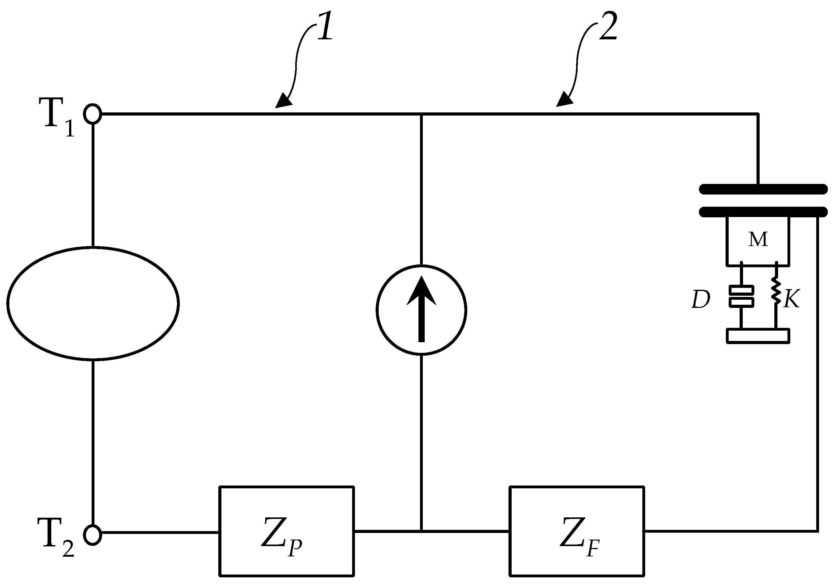
Figure 2.
Equivalent electrical diagram of an excitable membrane (3) in Figure 1.
Figure 2.
Equivalent electrical diagram of an excitable membrane (3) in Figure 1.
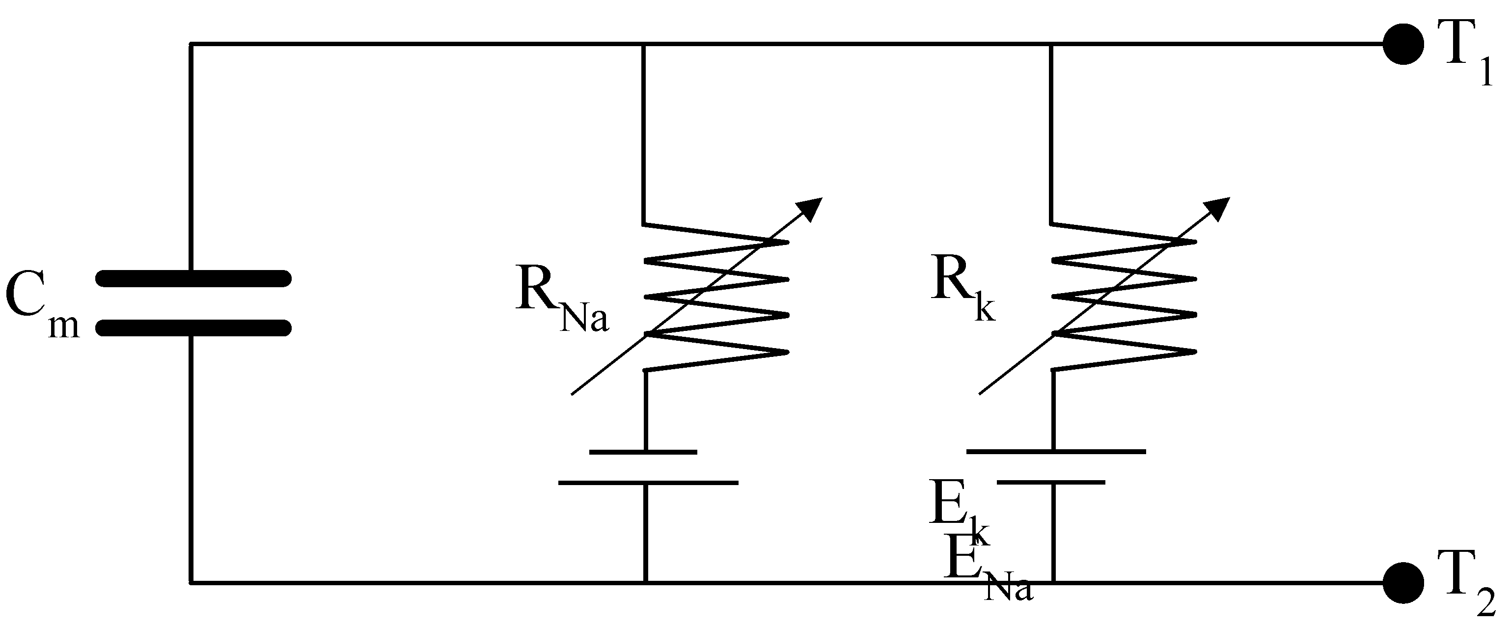
Figure 3.
Starting from the row on top, cell membrane potential, gating variables, changes in conduction of K+ and Na+ with the action potential, plotted versus time and with .
Figure 3.
Starting from the row on top, cell membrane potential, gating variables, changes in conduction of K+ and Na+ with the action potential, plotted versus time and with .
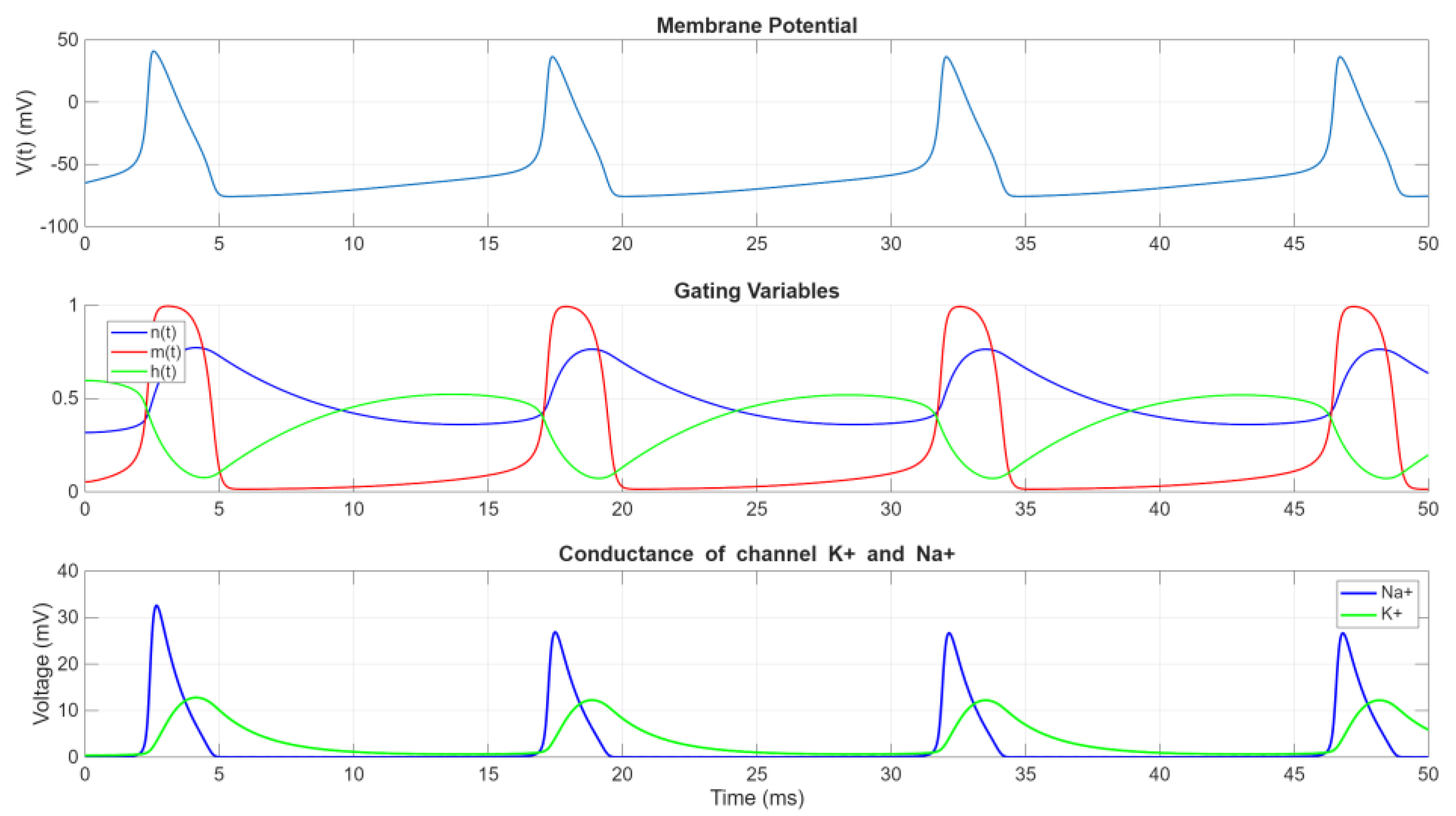
Figure 7.
Cell membrane potential, displacement and velocity of the resonator versus time.
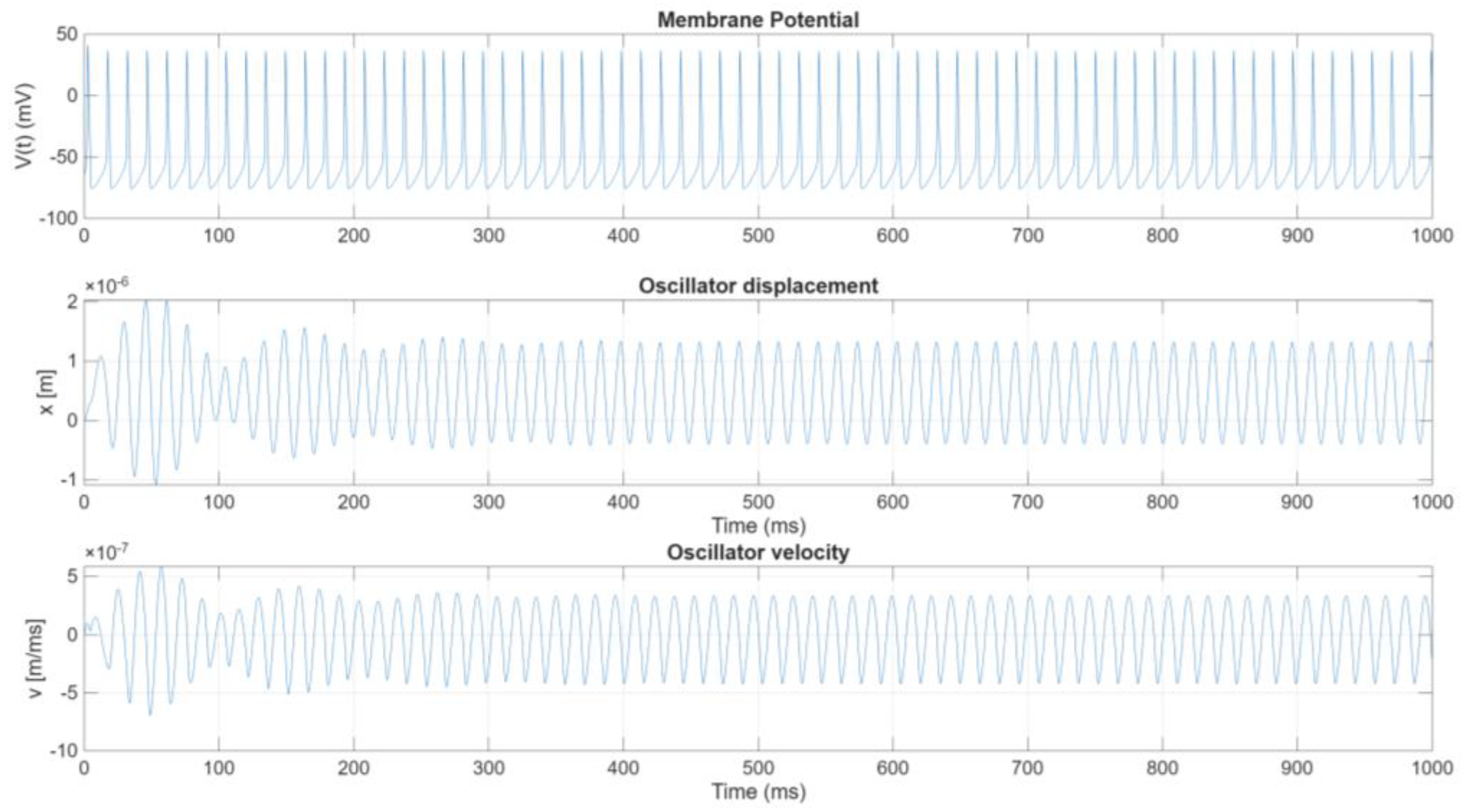
Figure 8.
Normalized FFT of the membrane potential (in blue line) and of the displacement of the mechanical oscillator system (in red). Normalization is performed by dividing each time signal by its maximum amplitude.
Figure 8.
Normalized FFT of the membrane potential (in blue line) and of the displacement of the mechanical oscillator system (in red). Normalization is performed by dividing each time signal by its maximum amplitude.
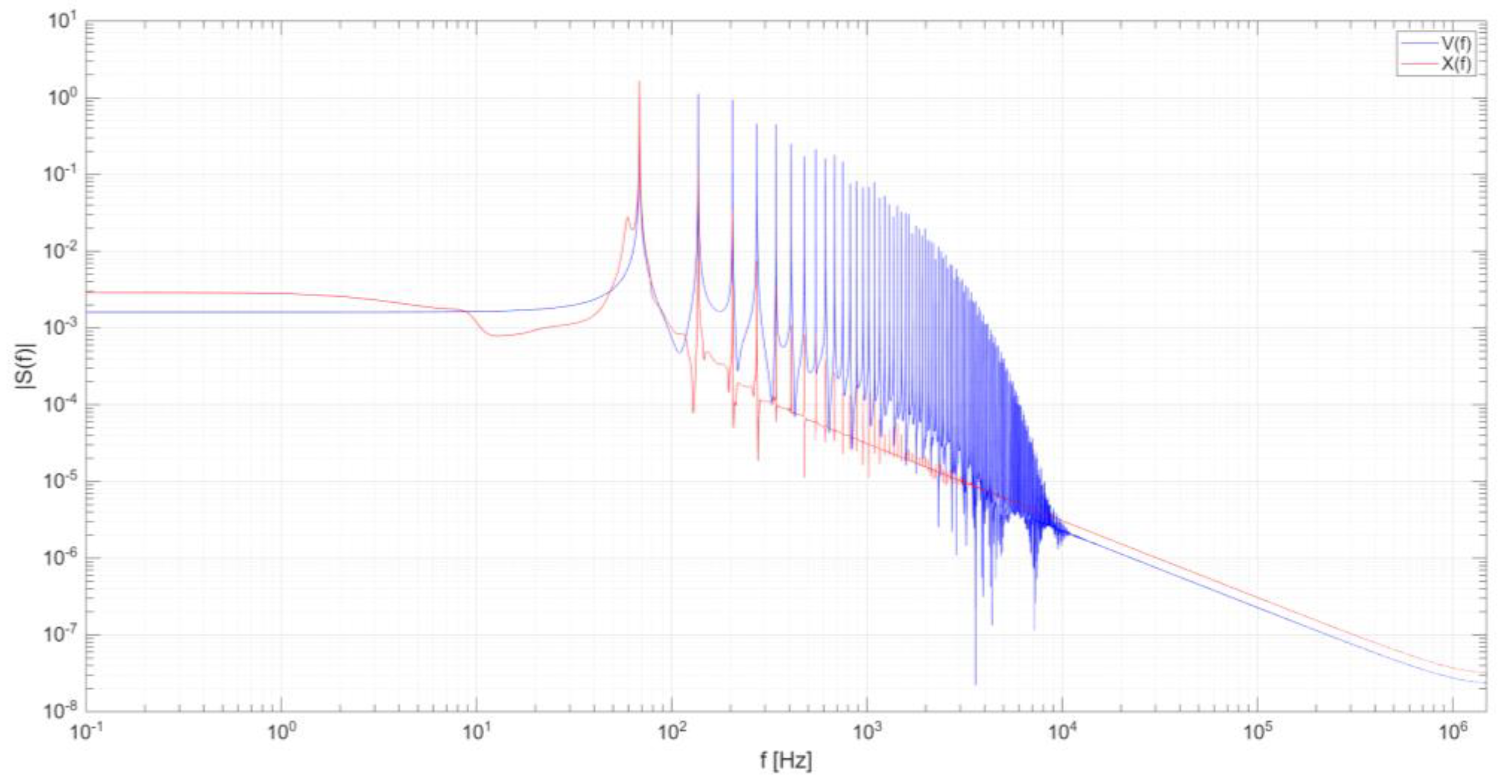
Figure 9.
Power components during a single charge-discharge cycle, organized into three subplots with different y-axis scales: (top) ionic power contributions (, , , and capacitive power (), (middle) external power (), and (bottom) power associated with the mechanical oscillator.
Figure 9.
Power components during a single charge-discharge cycle, organized into three subplots with different y-axis scales: (top) ionic power contributions (, , , and capacitive power (), (middle) external power (), and (bottom) power associated with the mechanical oscillator.
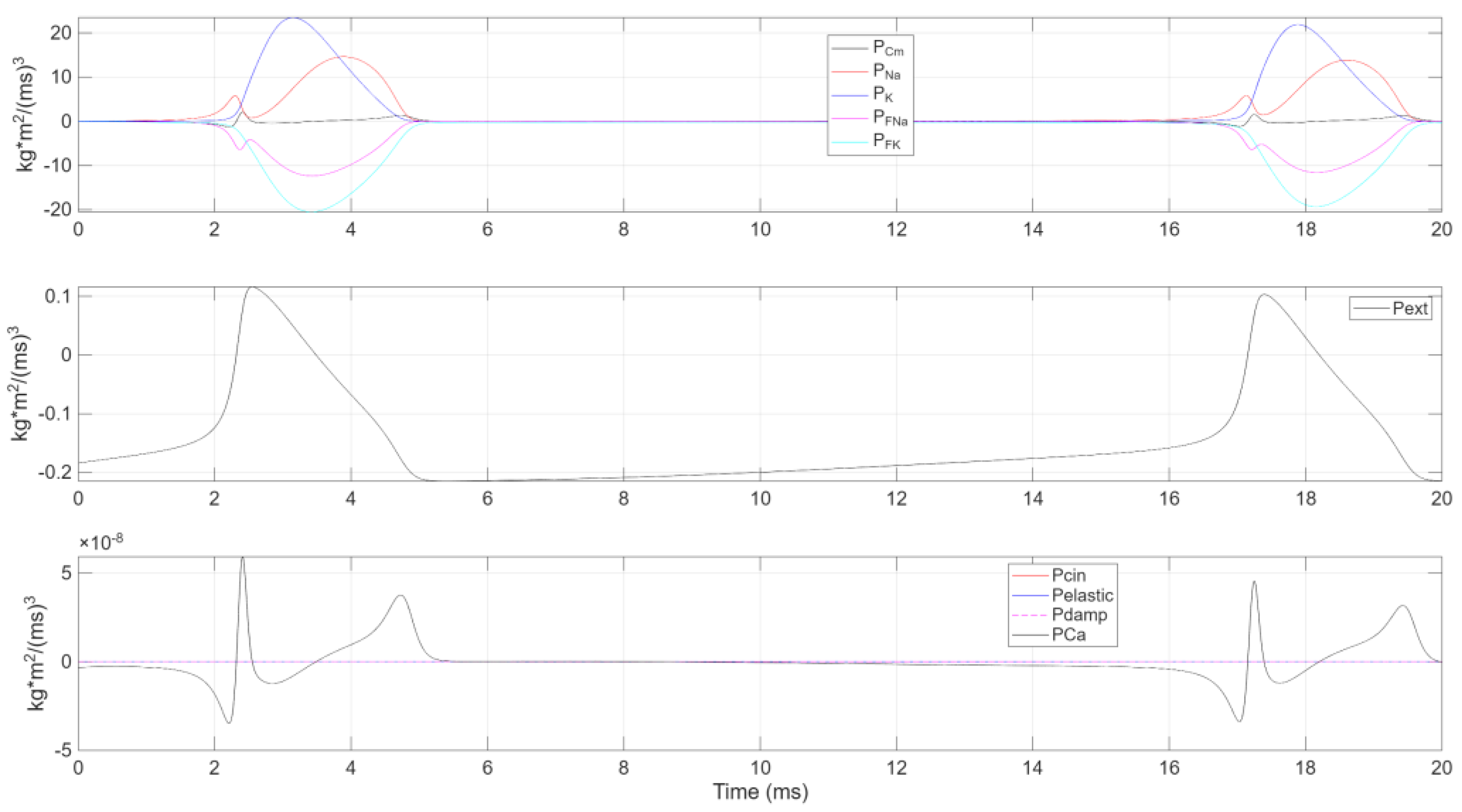
Figure 10.
Cell membrane potential, Displacement and velocity of the resonator plotted versus time with
Figure 10.
Cell membrane potential, Displacement and velocity of the resonator plotted versus time with
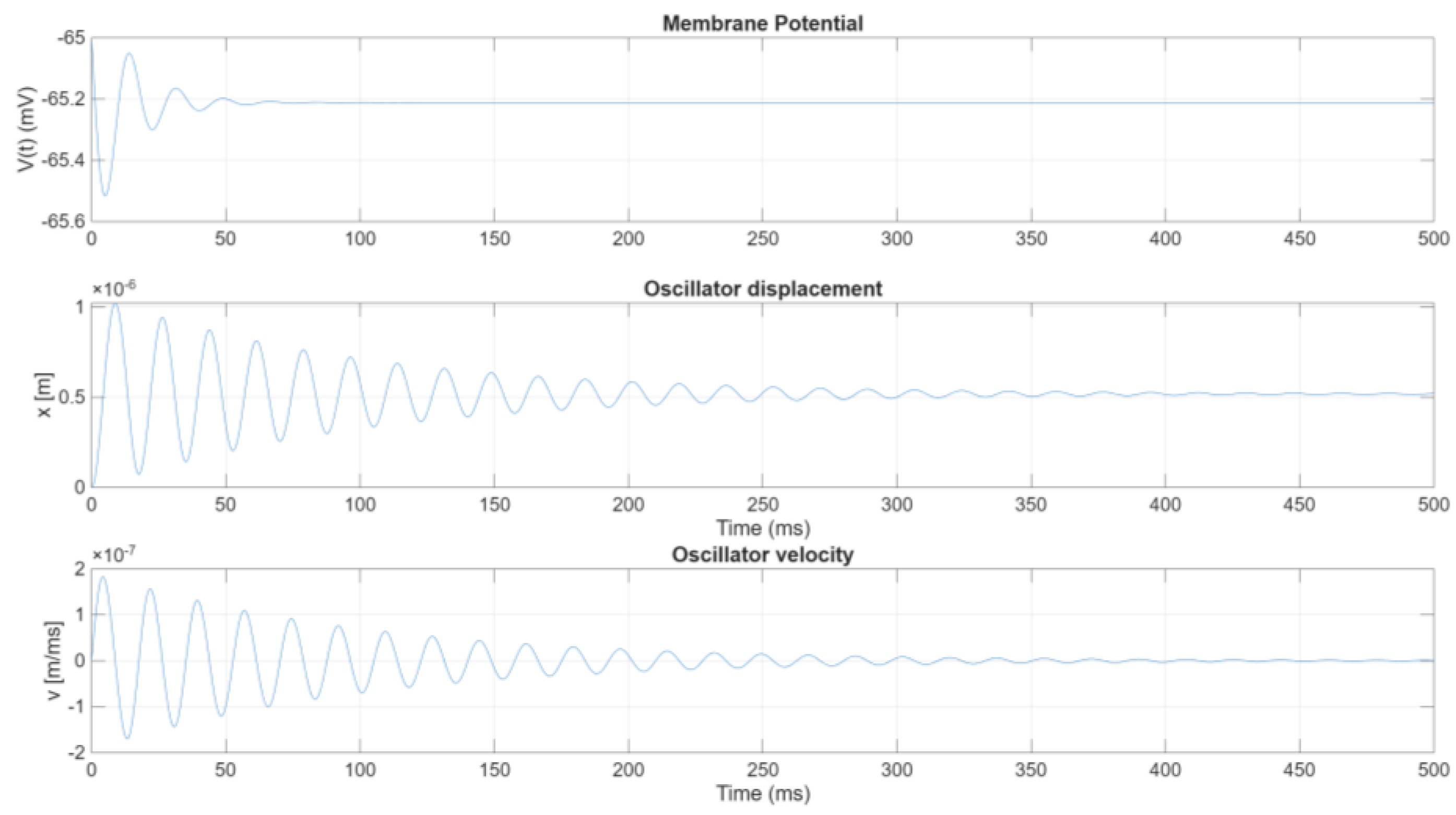

Table 1.
Equations used to define the gating variables.
| h | ||
| m | ||
| n |
Table 2.
The constant parameters of the Hodgkin-Huxley model.
| [mV] | ||
| 115+ | 120 | |
| -12+ | 36 |
Disclaimer/Publisher’s Note: The statements, opinions and data contained in all publications are solely those of the individual author(s) and contributor(s) and not of MDPI and/or the editor(s). MDPI and/or the editor(s) disclaim responsibility for any injury to people or property resulting from any ideas, methods, instructions or products referred to in the content. |
© 2025 by the authors. Licensee MDPI, Basel, Switzerland. This article is an open access article distributed under the terms and conditions of the Creative Commons Attribution (CC BY) license (http://creativecommons.org/licenses/by/4.0/).
Copyright: This open access article is published under a Creative Commons CC BY 4.0 license, which permit the free download, distribution, and reuse, provided that the author and preprint are cited in any reuse.


