
Submitted:
03 February 2025
Posted:
04 February 2025
You are already at the latest version
Abstract
This paper proposes an accuracy enhancement method for the fiber-longitudinal power profile estimation (PPE) based on convolutional neural networks (CNN). Two types of CNNs are designed. The first one is a network that treats different polarization streams identically. This network is denoted as CNN. The second one considers the difference between the contributions of different polarization streams to the nonlinear phase shift and is denoted as enhanced CNN (ECNN). The numerical simulation results confirm the effectiveness of the method for a 64 GBaud/s DP-QPSK system with a fiber length of 320 km. The effects of finite impulse response filter (FIR) length, power into the fiber, and polarization mode dispersion on the PPE accuracy are examined. Finally, monitoring results of the proposed method in the presence of several simultaneous power attenuation anomalies in the fiber optic link are shown. It is found that the accuracy of the PPE substantially improves after using the proposed method, achieving a relative gain of up to 71%.
Keywords:
fiber optics communications
; fiber-longitudinal power profile estimation
; convolutional neural networks
; nonlinear phase shift
; power attenuation anomalies
1. Introduction
Robust optical performance monitoring (OPM) plays a crucial part in the reliable operation of modern optical networks, which are evolving towards agile, disaggregated, and dynamic networks [1,2]. In recent years, a new OPM technology, called the fiber-longitudinal power profile estimation (PPE), has attracted a significant amount of attention [3,4]. It is based upon the idea of digital longitudinal monitoring (DLM), where “digital” indicates that the monitoring function is performed using digital signal processing (DSP) at the receiver side, and “Longitudinal” refers to the distributed monitoring of key parameters along the fiber optic link. So far, the DLM-based OPM can monitor the following parameters: optical power profile [5], chromatic dispersion (CD) [6], amplifiers’s gain tilt [7], optical filter detuning [8], optical-signal-to-noise ratio (OSNR) [9], polarization-dependent loss (PDL) [10], and differential group delay (DGD) [11]. The DLM-based optical power profile estimation, often abbreviated either as fiber-longitudinal PPE or In-site PPE, can predict the power evolution along an optical link in a distributed manner. The advantage of fiber-longitudinal PPE over optical time-domain reflectometer (OTDR) is that no dedicated equipment is needed to carry out manual on-site span-by-span measurement. For these reasons, it is chosen as the research topic in this paper.
According to [4], the existing fiber-longitudinal PPE can be classified into two main types: correlation-based methods (CMs) and minimum-mean-square-error-based methods (MMSEs). It was analytically shown in [4] that the CM-based methods have limited spatial resolution and measurement accuracy, even in noise- and distortion-free environments. On the other hand, the MMSE-based methods are not restricted by this limitation. There are a number of variants of the MMSE-based methods, such as Volterra-based MMSE [12], linear least squares (LS) [13] and deep-learning networks [14]. In terms of oversampling rate for signal reconstruction, fiber-longitudinal PPE can be classified into waveform-level and symbol-level methods [15]. In the waveform-level methods, the reference signal is oversampled by two times, whereas in the symbol-level methods, do not involve any up-sampling.
For the fiber-longitudinal PPE, the emulation of a fiber optic channel has a crucial impact on the estimation accuracy, especially for deep-learning based methods. It is well known that the propagation of an optical signal in an optical fiber follows a nonlinear Schrödinger equation. The LS-based analytical estimation methods usually establish a fiber channel emulator based on the regular perturbative solution of the nonlinear Schrödinger equation [13]. On the contrary, the deep learning-based methods usually create an artificial neural network that emulates the fiber optic channel according to the split-step Fourier (SSFM) algorithm for the nonlinear Schrödinger equation. For example, an optical fiber channel emulator using a deep learning network (DNN) was proposed by [3], which leveraged asymmetric SSFM to implement fiber-longitudinal PPE. The authors in [16] designed a double-effect digital back propagation (DBP) algorithm, which was actually a DNN, to simultaneously enable data communication and sensing of nonlinear fiber parameters. However, the correlation between the signal power of neighboring symbols when constructing the DNNs was ignored in both [3] and [16]. It is well known that chromatic dispersion causes an optical pulse to spread as it propagates through an optical fiber, which “spills” the optical signal power into neighboring symbols. The nonlinear phase shift at a specific symbol location is correlated with the power of multiple consecutive symbols, rather than only one. Furthermore, optical signals from different polarization streams contribute differently to the nonlinear phase shift [17]. Such phenomenon may be used to enhance the robustness of fiber channel emulators and improve the PPE estimation accuracy. However, only a few studies exist on this topic.
In order to cover this research gap and further enrich the fiber-longitudinal PPE implementation methods, this paper proposes a fiber channel emulator based on convolutional neural networks (CNNs). It can account for the overlap of the power of consecutive symbols and the discrepancy between the different polarization streams. The research results demonstrated in this paper suggest that the emulator can be successfully employed with fiber-longitudinal PPE, and is applicable to 64 GBaud/s fiber optic transmission systems. The rest of this paper is organized as follows: Section 2 presents the overall framework of the method. The design philosophies of the channel emulator and the signal processing flow at the receiver side are described. Section 3 describes in detail the numerical simulation methodology for the DP-QPSK fiber optic transmission system, and provides the key parameters of the CNNs. The influences of polarization mode dispersion (PMD) and fiber launch power are carefully analyzed, and the variation in the PPE accuracy with and without the CNNs is also compared. The paper is concluded in Section 4.
2. Principles of the Fiber-Longitudinal PPE Based on CNN
The method used for constructing the channel emulator is vital to improving the accuracy of PPE. The channel emulator is actually a virtual and digital counterpart of a real fiber that simulates the reverse transmission of a signal. When the generated optical signal is launched into a standard single mode fiber (SSMF), its propagation satisfies the nonlinear Schrödinger equation. Due to the random variation and coupling of the state of polarization (SOP) in a long-haul SSMF, the following Markov equation is considered here instead of the Markov-PMD equations:
Here, , with representing the optical signal waveform on the x polarization stream, and representing the y polarization stream. Subsequently, represents the optical signal power. is the fiber attenuation coefficient, is the CD coefficient an is the nonlinear coefficient. Let , which is substituted into (1) to obtain
The reverse propagation of the signal in the virtual fiber is numerically approximated in the digital domain using the DBP based on the SSFM algorithm. That is, the virtual fiber is divided into many sections and its parameters are inverse of those of the real fiber. Within each section, the linear and nonlinear parts of (2) are executed independently of each other. The linear part corresponds to the dispersion effect and is implemented in the frequency domain as follows:
where FFT stands for the Fourier Transform, represents the step size of each section and IFFT stands for the Inverse Fourier Transform. The nonlinear part corresponds to the Kerr nonlinear effect, implemented in the time domain as
The shortcoming of (5) is ignoring of the interaction between dispersion and nonlinearity. The term in (5) represents the summed power of the symbols at a given time slot. If dispersion is not considered, the propagating optical signal’s shape does not broaden, and the powers of different symbols do not overlap with one another. Thus, the nonlinear phase shift at a certain time slot is only related to the power of the current symbol. In reality, the chromatic dispersion should not be ignored, as the chromatic dispersion of optical fibers could cause the optical signals to broaden as they propagate. It causes the powers of different symbols to overlap at a given time slot location. Accordingly, the nonlinear phase shift must account for the power of the different symbols overlapping simultaneously in one time slot. Taking this phenomenon into account, (5) is modified as follows:
where is an odd integer representing the number of symbols used to account for a nonlinear phase shift, and is the real-valued weight coefficient. Furthermore, the intra-polarization and inter-polarization symbols contribute differently to the nonlinear phase shift. Consequently, (6) is modified as
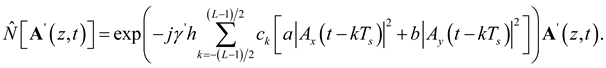 For the x polarization, and denote the intra-polarization and inter-polarization parameters, respectively, while for the y polarization, the parameters are reversed.
As there are similarities between the computational architectures of an SSFM and an artificial neural network [18], this paper converts the channel emulators described by Eqs. (5)-(7) to artificial neural networks as shown in Figure 1. The inputs of these neural networks are time-domain waveforms sampled at the rate of 2 samples/symbol. Each neural network consists of many layers. Based on Eqs. (5)-(7), three types of networks with different types of layer structures are designed, as shown in Figure 2. In the following these neural networks are discussed:
1)The first one is illustrated in Figure 2 (a), which is actually an ordinary DNN that contains a linear operator given by (4) and a nonlinear operator given by (5).
2) The second one is designed according to (6). It considers the powers of consecutive symbols when calculating a nonlinear phase shift. The summing operation in (6) used for computing a nonlinear phase shift is equivalent to the convolution of the signal power and a finite impulse response filter (FIR) that has taps. The tap coefficient of the FIR is denoted as . Figure 2 (b) shows the final outcome, i.e., a convolutional layer is inserted between the dispersion and the nonlinear phase-shift sections. It is referred to as a CNN in this paper.
3) To further enhance the estimation accuracy of PPE, the third type of neural network accommodates the difference between the contributions of different polarization symbols to a nonlinear phase shift. It is constructed according to (7) and shown in Figure 2 (c). It can be noted from the figure that the intra- and inter-polarization contributions in this neural network are denoted by and , respectively. This paper refers to this third type of neural network as an enhanced CNN (ECNN).
As Figure 1 shows, after handling dispersion and nonlinearity, the waveforms sampled at 2 samples/symbol are down-sampled to 1 sample/symbol. The last stage of these neural networks, as shown in Figure 1, involves a phase rotation with the reference symbols given by the waveform reconstruction module, which eliminates the residual constellation phase offset. During the network training process, the mean square error (MSE) between the symbols output by these neural networks and the reference symbols is used as the loss function. That is, , where and are the symbols on the two polarization streams of each neural network’s output, and and are the reference symbols. The effective SNR for symbols is defined as follows:
where is the number of symbols contained in a waveform sample, is the number of training epochs, and is the mini-batch size. The trainable network parameters are denoted by , , and , which are optimized by minimizing the MSE using the Adam optimizer.
Figure 3 shows the holistic configuration of the fiber-longitudinal PPE based on the proposed CNN. A typical long-haul DP-QPSK coherent fiber optic transmission system is considered in this method, but the signal processing is tailored for both the transmitter and receiver sides. The DSP in the transmitter primarily consists of QPSK symbol mapping, pulse shaping, and digital pre-emphasis. Figure 3 shows the DSP for implementing PPE in a coherent receiver. First, the electrical signal is matched-filtered and resampled. Second, the output signal goes through CD compensation, adaptive equalization using the Least-Mean-Square (LMS) algorithm, and pilot-assisted CPR, respectively. A perfect compensation of the frequency offset is assumed in this study. After CPR, the DSP in the coherent optical receiver is divided into upper and lower branches. In the former, the signal passes through the DSP chain for reference waveform reconstruction. As Figure 3 shows, the residual phase noise (RPN) within the signal is estimated and compensated in the upper branch, and subsequently, a symbol decision is rendered. Next, the reference symbols reloaded with RPN are produced and fed into the CNNs in the waveform reconstruction module. In the lower branch, the signal output from the CPR is reloaded with the CD, divided into batches, and finally fed into the channel emulator as depicted in Figure 1 and Figure 2 for DBP.
3. Simulation Results and Discussion
Figure 3 shows a numerical simulation platform for polarization multiplexing (PDM) M-QAM coherent optical communication system constructed to validate the effectiveness of the proposed method. It has a symbol rate of 64 GBaud/s and a modulation format of QPSK. The fiber optic link of this system is made up of multiple spans, with the number of fiber spans and the fiber length per span denoted as and , respectively. The fiber under consideration has a nonlinear index of 2.6×10⁻²⁰ m2/W and a dispersion parameter of 17 ps/nm/km. The PMD coefficient varies between 0.01 and 0.1 ps/sqrt(km). When the forward transmission of an optical signal is simulated over a real long-haul fiber, the asymmetric SSFM is used to handle the dispersion and Kerr nonlinear effects. In addition, a coarse-step approximation method is used to simulate the polarization-related effects [19]. This method is also referred to as a waveplate model. The total line-width of the transmitter laser and the local oscillator is fixed at 10 kHz. The noise figure of Erbium-doped fiber amplifiers (EDFA) is chosen as 4 dB. The total CD accumulated on the fiber optic link is perfectly compensated with an electric domain DSP incorporated in the receiver. A frequency domain filter is used here. The random revolutions of SOP and the PMD are equalized using a data-aided LMS algorithm with 32 taps [20].
The neural networks shown in Figure 1 and Figure 2 are built using TensorFlow, and the learning rate of the three neural networks is fixed at 0.0001. The impairment-contaminated waveforms and the reference symbols output by the waveform reconstruction module are simultaneously fed into the three neural networks for training and parameter optimization. The Adam optimizer is used to minimize the loss function during 100 iterations. In each iteration, 10 waveforms are randomly selected out of a total of 1000 waveform samples and input into the three neural networks for training. Each iteration runs for 200 epochs. The final longitudinal power profile output by the three neural networks is obtained by averaging the results over 100 iterations.
First, the performance of the three different neural networks shown in Figure 2 is examined in terms of the PPE accuracy. In this example, the total distance of the fiber optic link is 320 km, including four spans of 80 km each. When the SSFM algorithm is mapped to a neural network, each fiber span is partitioned into forty steps. It is assumed that there are no anomalous attenuation spots on the overall fiber optic link. The average optical power into the fiber is temporarily fixed at 3 dBm. The filter length for the two CNNs shown in Figure 2 (b) and (c) is chosen as 5 temporarily. The theoretical power profile is compared with that estimated by the proposed method at each spatial location.
All results are presented in Figure 4 (a). In this figure, the DNN results are indicated by the solid line with triangular symbols, and the CNN results are marked by a solid line with square symbols. The ECNN results, on the other hand, are indicated by a solid line with circular symbols. As Figure 4 (a) shows, the PPE accuracy of the DNN deteriorates considerably at the beginning and end of each fiber span. After using the proposed ECNN, the PPE accuracy at these locations is noticeably improved. In order to more clearly compare the performance of the three neural networks, the absolute error of PPE is computed at each spatial location as , where is the theoretical power profile at position , and is the power profile estimated by the proposed method. Figure 4 (b) shows the obtained results, where it can be observed that the DNN results in the worst PPE accuracy, followed by the CNN. The ECNN performs the best, giving the highest PPE accuracy.
Second, the impact of the FIR filter length is investigated on the PPE performance of the ECNN. The fiber span number, length per span, and the power into the fiber remain unchanged from the previous section. The FIR filter length for CNNs is increased from 3 to 11 at intervals of 2. The PPE accuracy is quantified using the mean squared deviation (MSD) metric calculated as shown below:
where is the number of spatial positions . For each filter length, the power profile is calculated ten times for this fiber link based on the proposed ECNN. Subsequently, the MSD for each power profile is derived according to (9). All the obtained results are shown in Figure 5, where the box plots are superimposed upon a scatter plot to provide the statistical distribution of these ten measurements. Each point in the figure represents one MSD of a power profile. The average of these ten measurements is also marked in bold red beside the box plot. It can be observed that the ECNN performs the best in terms of the PPE when the filter length is equal to 5, i.e., the optimal length of the FIR filter is equal to 5. Furthermore, the average MSD of PPE given by the ECNN is the minimum at only 0.13575. The PPE performance of the ECNN will degrade when the FIR filter length is less than or greater than 5. Therefore, the FIR filter length of CNNs is selected as 5 in the following experiments, unless stated otherwise.
Third, the impact of different optical power values into the fiber and PMD coefficients on the accuracy of PPE are investigated. For this purpose, the optical power into the fiber is increased from -2 dBm to 8 dBm, and the PMD coefficient of SSMF is chosen as 0.02 ps/sqrt(km). The fiber span number and length per span are kept the same as those in the earlier experiment. For each power value, the power profile of the fiber link is estimated using the DNN, CNN, and ECNN shown in Figure 2. Figure 6 (a) shows the corresponding MSDs. It can be observed that the PPE accuracy of DNN continuously degrades as the power into the fiber gradually increases. After incorporation of the convolutional layer in the neural network, the accuracy of PPE shows an obvious improvement. The PPE performance exhibited by the CNN and ECNN is significantly less dependent on the power transmitted into the fiber. The PPE accuracy of the latter is superior to that of the former. When the power is increased from -2 dBm to 8 dBm, the average relative improvement of the MSD of ECNN can be up to 71% with respect to that of the DNN.
To investigate the influence of the PMD coefficient, the power into the fiber is fixed at 3 dBm, while the PMD coefficient is increased from 0.02 to 0.20 ps/sqrt(km) at intervals of 0.03 ps/sqrt(km). For each PMD coefficient, the MSDs of the PPE output from the three neural networks are shown in Figure 6 (b). Comparing Figure 6 (a) and (b), it can be noted that the PMD coefficient has a considerably smaller impact on the PPE accuracy than the power into the fiber. The MSDs of PPE are almost invariant, showing minor variations with respect to the PMD coefficients. At a given PMD coefficient, the ECNN has the highest PPE accuracy, followed by the CNN and the DNN.
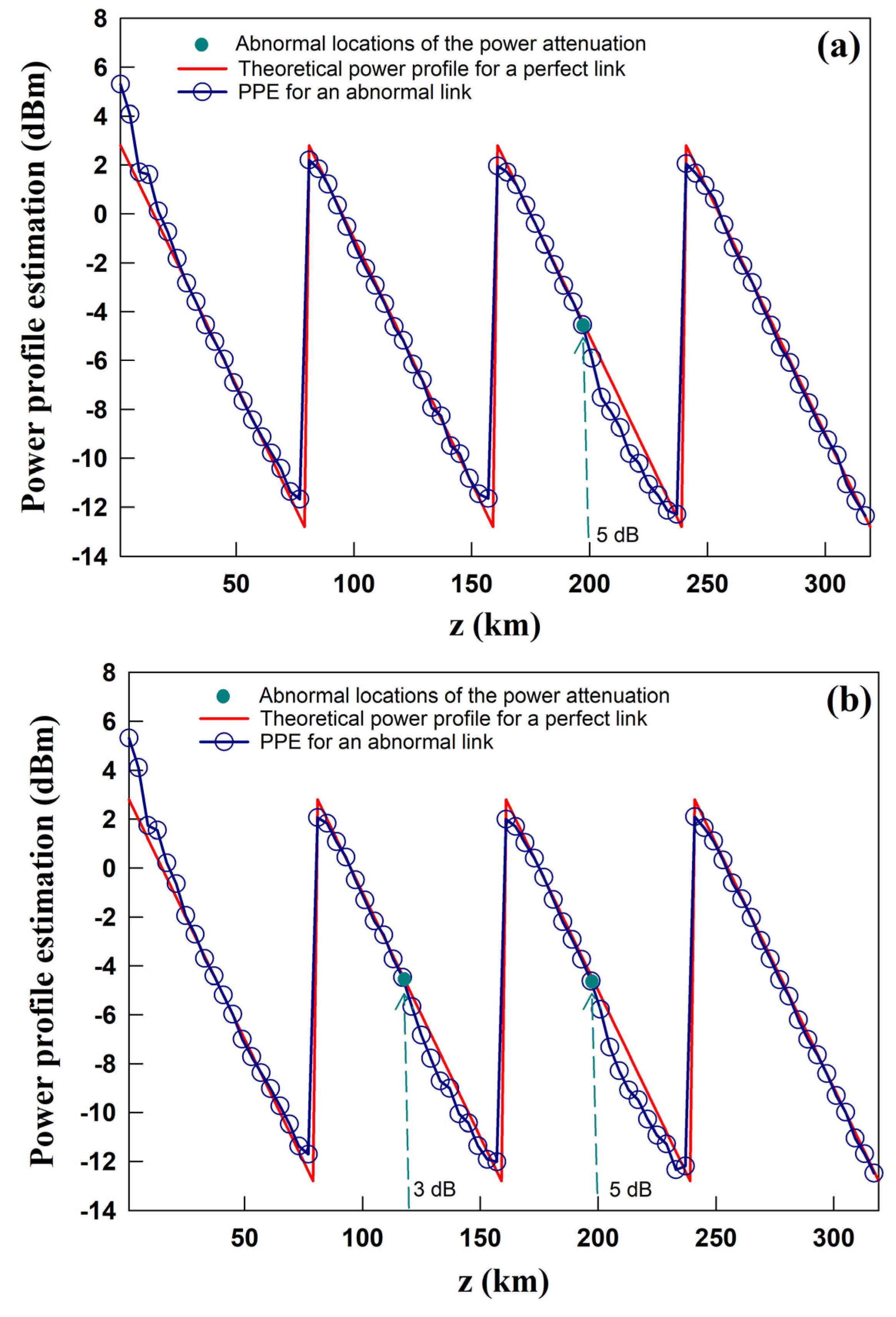
Last, the PPE capability of the proposed method is verified for abnormal fiber links. The fiber span number and the length of fiber per span remain unchanged. The power into the fiber is fixed as 3 dBm and the PMD coefficient is chosen as 0.02 ps/sqrt(km). It is assumed that the EDFA operates in the constant output power mode. Two abnormal scenarios are considered and the PPE performance of the proposed method is verified in these scenarios. The first scenario involves the appearance of a power attenuation anomaly of 5 dB right in the middle of the third fiber span. In the second scenario, two power attenuation anomalies of 3 dB and 5 dB occur simultaneously in the middle of the second and third fiber spans, respectively. The PPE results output from the proposed ECNN corresponding to the two scenarios are shown in Figure 7 (a) and (b), respectively. The actual locations where power attenuation anomalies occur are marked with cyan dots in these figures. It can be observed that at these abnormal locations, the ECNN outputs and the theoretical results deviate significantly, which indicates that the proposed method can detect the power anomalous attenuation successfully in both scenarios.
4. Conclusions
In summary, the paper proposed accuracy improvement of a fiber-longitudinal PPE using a CNN-based method. The working principle, optimization approach, and construction of CNN were first discussed in detail. Moreover, it elaborated on the signal processing of the corresponding fiber-longitudinal PPE. The efficiency of the proposed method was verified by the numerical simulation of a 64 GBaud/s DP-QPSK coherent fiber optic transmission system. It was verified that the power into the fiber and PMD had a minor influence on the proposed method. The accuracy of PPE was substantially improved by using the proposed method, compared to without using it. The proposed method could correctly estimate the anomalous locations of several power attenuation anomalies on the fiber link. The results of this paper can prove to be a useful contribution to the development of DLM-based optical performance monitoring technology.
Author Contributions
Conceptualization, D.W. and K.W.; methodology, K.W. and T.B.; software, K.W. and T.B.; validation, K.W. and T.B. and R.X.; formal analysis, D.W. and Z.Z.; investigation, K.W.; resources, T.B.; data curation, K.W.; writing—original draft preparation, D.W. and T.B.; writing—review and editing, D.W., T.B., K.W. and G.G.; visualization, K.W. and D.W.; supervision, D.W.; project administration, D.W.; funding acquisition, G.G. and D.W. All authors have read and agreed to the published version of the manuscript.
Funding
This work was supported in part by National Key Research and Development Program of China (2022YFB2903303) and National Natural Science Foundation of China (No. 62141505, 61367007 and 62371064).
Institutional Review Board Statement
Not applicable.
Informed Consent Statement
Not applicable.
Data Availability Statement
The data used to support the findings of this study are available from the corresponding author upon request.
Conflicts of Interest
The authors declare no conflict of interest.
References
- Saif, W.; Esmail, M. Machine Learning Techniques for Optical Performance Monitoring and Modulation Format Identification: A Survey. IEEE Commun. Surv. Tutor. 2020, 22, 2839–2882. [Google Scholar] [CrossRef]
- Wang, D.; Jiang, H. Optical Performance Monitoring of Multiple Parameters in Future Optical Networks. J. Light. Technol. 2021, 39, 3792–3800. [Google Scholar] [CrossRef]
- Sasai, T.; Nakamura, M. Digital Longitudinal Monitoring of Optical Fiber Communication Link. Journal of Lightwave Technology 2022, 40, 2390–2408. [Google Scholar] [CrossRef]
- Sasai, T.; Yamazaki, E. Performance Limit of Fiber-Longitudinal Power Profile Estimation Methods. J. Light. Technol. 2023, 41, 3278–3289. [Google Scholar] [CrossRef]
- Jiang, Y.; Tang, D. Low-complexity weighted regular perturbation model-based symbol rate power profile estimation. Opt. Express 2024, 32, 3526–3526. [Google Scholar] [CrossRef]
- Sasai, T.; Nakamura, M.; Okamoto, S. Simultaneous Detection of Anomaly Points and Fiber Types in Multi-Span Transmission Links Only by Receiver-Side Digital Signal Processing. In Proceedings of the 2020 Optical Fiber Communications Conference and Exhibition (OFC), San Diego, USA, 08-12 March 2020. [Google Scholar]
- Sena, M.; Emmerich, R. DSP-Based Link Tomography for Amplifier Gain Estimation and Anomaly Detection in C+L-Band Systems. J. Light. Technol. 2022, 40, 3395–3405. [Google Scholar] [CrossRef]
- Sasai, T.; Nakamura, M.; Yamazaki, E. Digital Backpropagation for Optical Path Monitoring: Loss Profile and Passband Narrowing Estimation. In Proceedings of the 2020 European Conference on Optical Communications (ECOC), Brussels, Belgium, 06-10 December 2020. [Google Scholar]
- Kim, I.; Sone, K.; Vassilieva, O. Nonlinear SNR Estimation based on Power Profile Estimation in Hybrid Raman-EDFA Link. In Proceedings of the 2024 Optical Fiber Communications Conference and Exhibition (OFC), San Diego, USA, 24-28 March 2024. [Google Scholar]
- Eto, M.; Tajima, K.; Yoshida, S. Location-resolved PDL Monitoring with Rx-side Digital Signal Processing in Multi-span Optical Transmission System. In Proceedings of the 2022 Optical Fiber Communications Conference and Exhibition (OFC), San Diego, USA, 06-10 March 2022. [Google Scholar]
- Hahn, C.; Chang, J.; Jiang, Z. Estimation and Localization of DGD Distributed Over Multi-Span Optical Link by Correlation Template Method. In Proceedings of the Optical Fiber Communication Conference (OFC) 2024, San Diego, United States, 24-28 March 2024. [Google Scholar]
- Gleb, S.; Konstantin, P.; Luo, J. Fiber Link Anomaly Detection and Estimation Based on Signal Nonlinearity. In Proceedings of the 2021 European Conference on Optical Communication (ECOC), Bordeaux, France, 13-16 September 2021. [Google Scholar]
- Sasai, T.; Takahashi, M. Linear Least Squares Estimation of Fiber-Longitudinal Optical Power Profile. J. Light. Technol. 2023, 42, 1955–1965. [Google Scholar] [CrossRef]
- Tanimura, T.; Yoshida, S. Concept and implementation study of advanced DSP-based fiber-longitudinal optical power profile monitoring toward optical network tomography [Invited]. J. Opt. Commun. Netw. 2021, 13, E132–E141. [Google Scholar] [CrossRef]
- Jiang, Y.; Tang, D. Symbol-level fiber-longitudinal power profile estimation. Opt. Lett. 2024, 49, 2305–2308. [Google Scholar] [CrossRef] [PubMed]
- Li, F.; Zhou, X. The DNN-based DBP scheme for nonlinear compensation and longitudinal monitoring of optical fiber links. Digit. Commun. Netw. 2023. [Google Scholar] [CrossRef]
- Rafique, D.; Mussolin, M. Compensation of intra-channel nonlinear fibre impairments using simplified digital back-propagation algorithm. Opt. Express 2011, 19, 9453–9460. [Google Scholar] [CrossRef] [PubMed]
- Häger, C.; Pfister, H. Physics-Based Deep Learning for Fiber-Optic Communication Systems. IEEE J. Sel. Areas Commun. 2021, 39, 280–294. [Google Scholar] [CrossRef]
- Marcuse, D.; Manyuk, C. Application of the Manakov-PMD equation to studies of signal propagation in optical fibers with randomly varying birefringence. J. Light. Technol. 1997, 15, 1735–1746. [Google Scholar] [CrossRef]
- Andrenacci, L.; Bosco, G. PDL Localization and Estimation Through Linear Least Squares-Based Longitudinal Power Monitoring. IEEE Photonics Technol. Lett. 2023, 35, 1431–1434. [Google Scholar] [CrossRef]
Figure 1.
Machine-Learning based fiber optic channel emulator used in this paper.
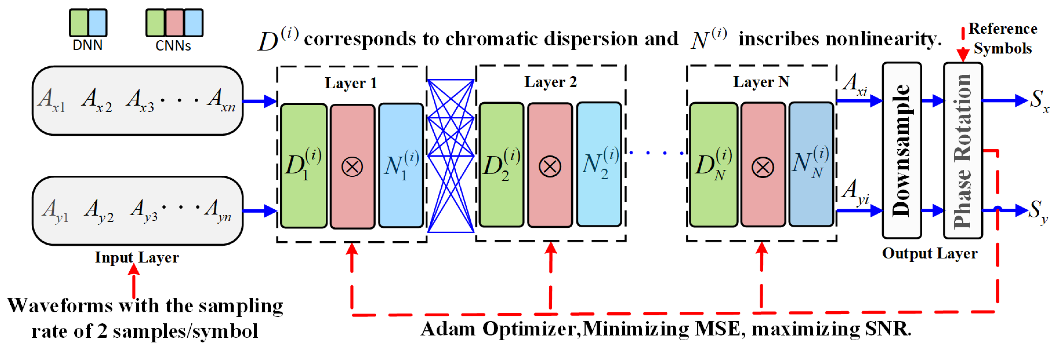
Figure 2.
Three neural network configurations used to realize fiber-longitudinal PPE, (a) DNN, (b) CNN, (c) ECNN.
Figure 2.
Three neural network configurations used to realize fiber-longitudinal PPE, (a) DNN, (b) CNN, (c) ECNN.
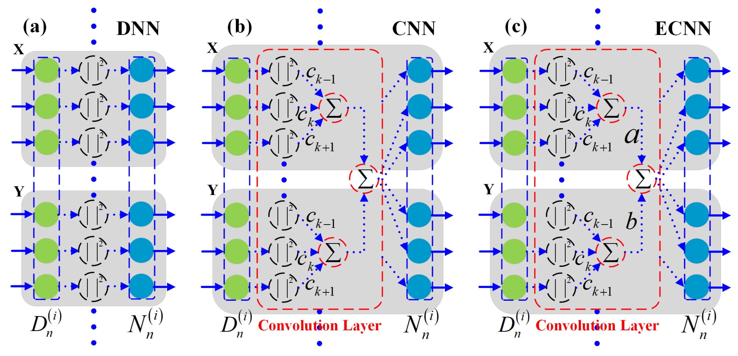
Figure 3.
Configuration of a coherent optical DP-QPSK transmission system and the DSP for fiber-longitudinal PPE.
Figure 3.
Configuration of a coherent optical DP-QPSK transmission system and the DSP for fiber-longitudinal PPE.
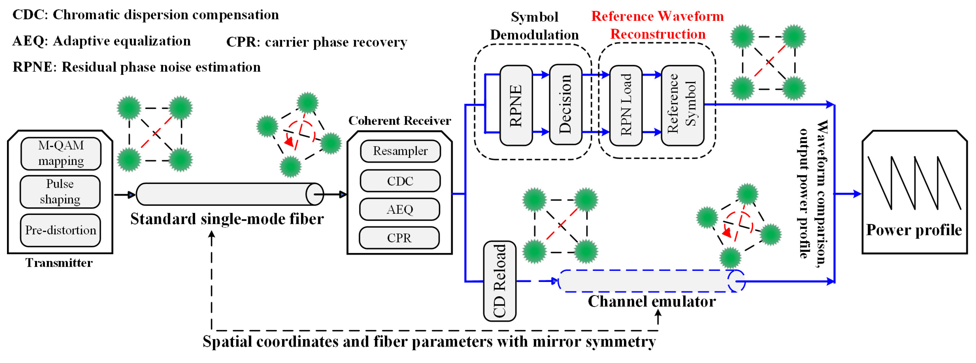
Figure 4.
Comparison of PPE results for three neural networks: (a) power profiles; (b) absolute errors between ideal and measured results for DNN, CNN and ECNN.
Figure 4.
Comparison of PPE results for three neural networks: (a) power profiles; (b) absolute errors between ideal and measured results for DNN, CNN and ECNN.
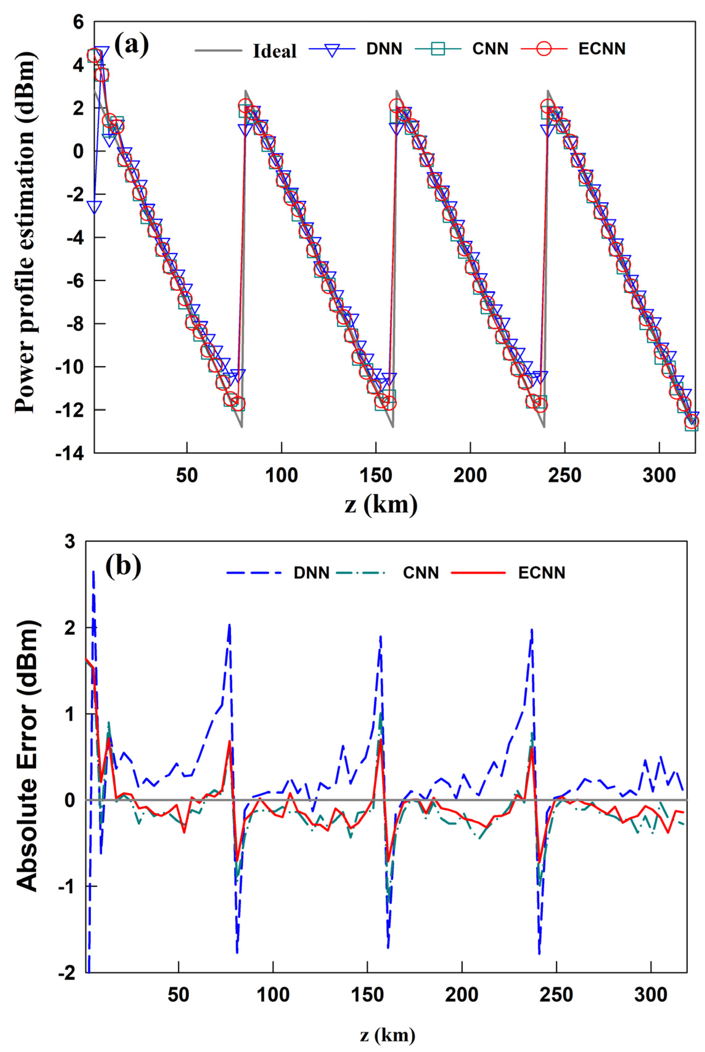
Figure 5.
Impact of the FIR filter length on the PPE performance of ECNN.
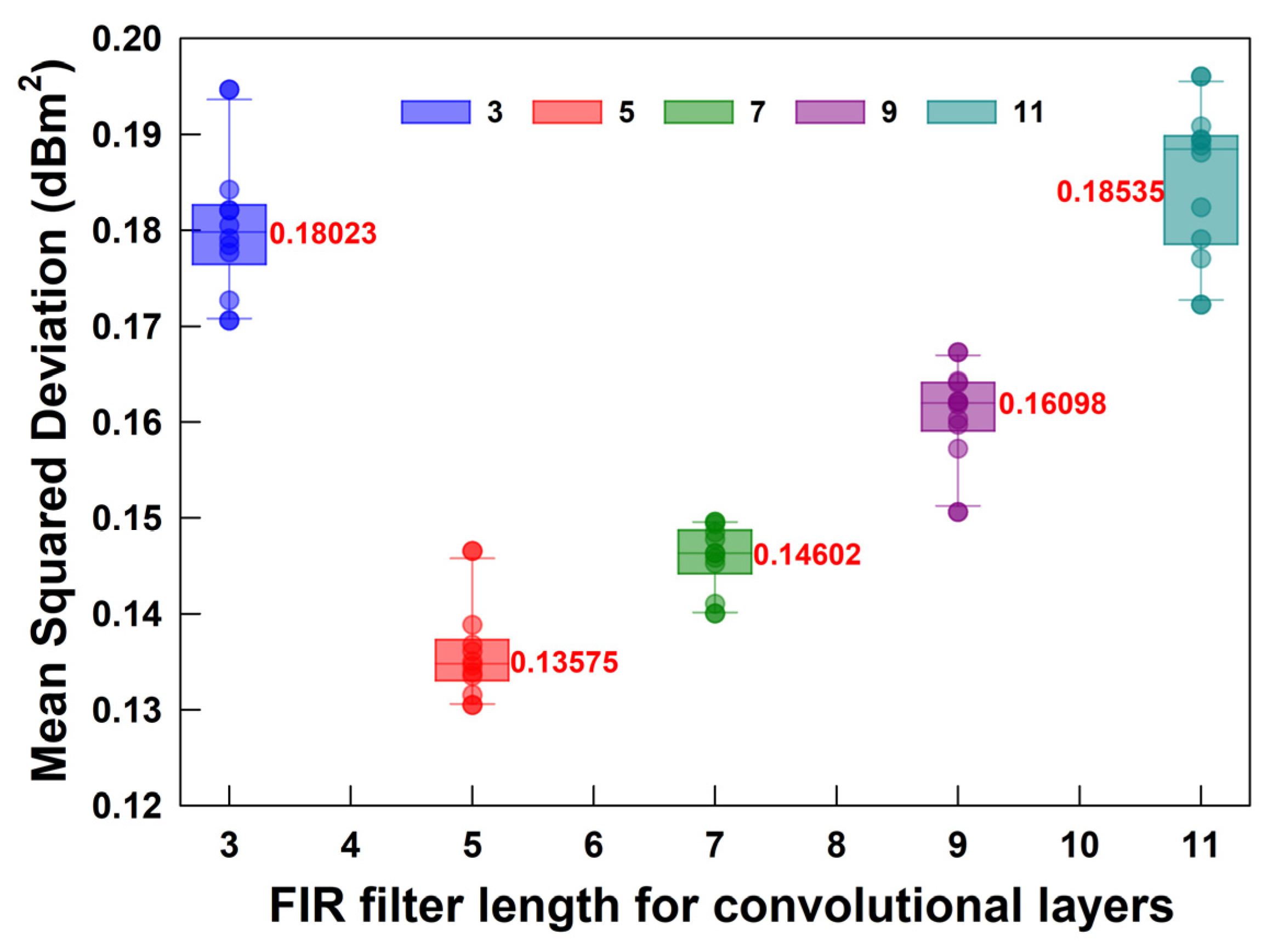
Figure 6.
Impact of the different optical power values into the fiber and PMD coefficients on the PPE performances of three neural networks: (a) optical power; (b) PMD coefficient of SSMF.
Figure 6.
Impact of the different optical power values into the fiber and PMD coefficients on the PPE performances of three neural networks: (a) optical power; (b) PMD coefficient of SSMF.
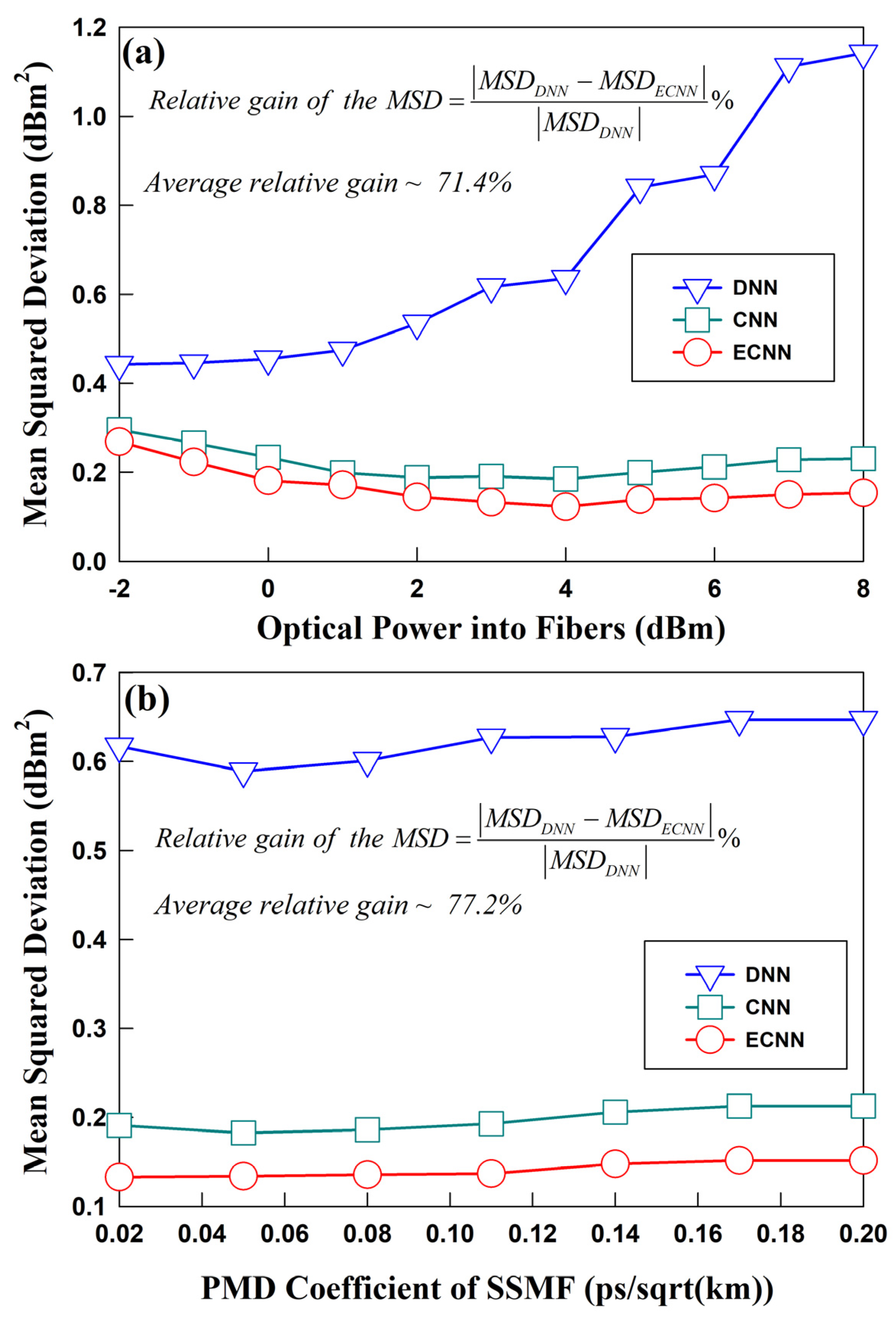
Figure 7.
Power profile estimation capability of the proposed method in the abnormal fiber link: (a) the scenario where only one power attenuation anomaly occurs; (b) the scenario where two power attenuation anomalies occur simultaneously.
Figure 7.
Power profile estimation capability of the proposed method in the abnormal fiber link: (a) the scenario where only one power attenuation anomaly occurs; (b) the scenario where two power attenuation anomalies occur simultaneously.
Disclaimer/Publisher’s Note: The statements, opinions and data contained in all publications are solely those of the individual author(s) and contributor(s) and not of MDPI and/or the editor(s). MDPI and/or the editor(s) disclaim responsibility for any injury to people or property resulting from any ideas, methods, instructions or products referred to in the content. |
© 2025 by the authors. Licensee MDPI, Basel, Switzerland. This article is an open access article distributed under the terms and conditions of the Creative Commons Attribution (CC BY) license (http://creativecommons.org/licenses/by/4.0/).
Copyright: This open access article is published under a Creative Commons CC BY 4.0 license, which permit the free download, distribution, and reuse, provided that the author and preprint are cited in any reuse.


