Submitted:
31 January 2025
Posted:
03 February 2025
You are already at the latest version
Abstract
We propose a geometric framework for cosmology by modeling the universe as a finite 3-dimensional hypersurface embedded in a static 4D bulk. Dynamic boundary interactions generate curvature gradients, quantified by a boundary tensor, which replaces dark energy in the Einstein equations. The theory resolves the Hubble tension via a radial Hubble parameter, predicts CMB quadrupole alignment, and matches large-scale structure observations. Derived from first principles, it eliminates singularities, satisfies energy conditions, and recovers general relativity as the boundary radius as R reaches infinity.Numerical solutions validate cosmic acceleration and observational consistency with lambda CDM.
Keywords:
cosmos
; expansion
; universe
; Lambdacdm
; boundary
1. Introduction
Modern cosmology rests on the twin pillars of Einstein’s general relativity and the CDM paradigm. While empirically successful, this framework faces persistent theoretical challenges: the unknown nature of dark energy, tensions in Hubble constant measurements [2,3], and the lack of a first-principles mechanism for cosmic acceleration. This work proposes a geometric resolution by unifying spacetime geometry with the boundary conditions of a finite universe.
We model the universe as a compact 3-manifold isometrically embedded in a static 4D Lorentzian bulk . Dynamic boundary interactions at generate intrinsic curvature gradients, quantified by the boundary tensor , which replaces dark energy in the modified Einstein equations:
Key features of this approach include:
- A finite universe topology with radius R, avoiding singularities through boundary curvature regularization (Section 3.6),
- Radial dependence in the Hubble parameter , naturally resolving the tension (Section 5.1),
- Emergent dark energy from extrinsic curvature, , without exotic fields,
- Compatibility with energy conditions and Machian inertia (Section 6).
The theory is observationally indistinguishable from CDM at intermediate scales but predicts testable signatures: a Hubble gradient (Eq. (126)), CMB quadrupole alignment (Section 5.6), and modified gravitational wave propagation (Eq. (179)). Numerical solutions (Figure 1) demonstrate consistency with cosmic acceleration and structure formation.
2. Foundational Principles
The theory rests upon three axiomatic principles, rooted in geometric intuition and mathematical consistency, which redefine the universe’s architecture and its interaction with boundaries:
2.1. Principle of Finite Embedding
- Manifold Structure: The universe is a compact orientable 3-manifold isometrically embedded in a 4-dimensional Lorentzian manifold (the bulk) via:where are bulk coordinates and are intrinsic coordinates.
- Induced Metric: The spacetime metric on is the pullback of the bulk metric :
- Normal Vector Field: The unit timelike normal vector satisfies:
- Extrinsic Curvature: The second fundamental form is defined as:where is the Lie derivative along .
2.2. Principle of Boundary Dynamics
- Boundary Action Principle: The total action contains boundary terms:where is the boundary induced metric.
- Israel Junction Conditions: At the boundary , the discontinuity in extrinsic curvature generates effective stress-energy:where is the surface stress-energy tensor.
- Boundary Tensor: From variational principle we derive:modifying Einstein’s equations to:
2.3. Principle of Geometric Unification
- Cosmic Acceleration: The boundary tensor generates effective dark energy:appearing in modified Friedmann equations:
- Conservation Laws: Energy-momentum conservation emerges from:proven via Codazzi identity:
- Topological Constraint: The Gauss-Bonnet theorem enforces:where is the Euler characteristic.
2.4. Example: 3-Sphere Universe
For a closed universe embedded in 4D Euclidean space:
- Embedding Coordinates:
- Induced Metric:
- Extrinsic Curvature Components:
- Effective Cosmological Constant:
3. Mathematical Framework
This section provides a rigorous derivation of the modified Einstein equations, boundary tensor, and cosmological solutions, grounded in differential geometry and variational principles.
3.1. Embedding and Induced Geometry
Let the universe be modeled as a 3-dimensional hypersurface smoothly embedded in a 4-dimensional Lorentzian bulk manifold . The embedding is governed by the following mathematical structure:
3.1.1. Bulk Metric and Embedding Functions
Let have coordinates () and metric . The embedding of into is defined by a set of smooth functions:
where () are coordinates on .
3.1.2. Induced Metric
The induced metric on is obtained by pulling back the bulk metric :
By the Nash embedding theorem, such an isometric embedding exists globally for smooth if is compact.
3.1.3. Normal Vector
The unit normal vector to satisfies:
3.1.4. Projection Tensor
The projection tensor , which maps bulk vectors to , is:
where .
3.1.5. Extrinsic Curvature
The extrinsic curvature tensor quantifies how bends in . It is derived from the Lie derivative of along :
where are Christoffel symbols of . In terms of the bulk covariant derivative :
3.1.6. Gauss-Codazzi Equations
The intrinsic and extrinsic geometry of are related by:
- Gauss equation (4D curvature ↔ 3D curvature + extrinsic terms):
- Codazzi equation (conservation of extrinsic curvature):
3.1.7. Topological Constraints
The compactness of implies:
- Finite volume:
- Gauss-Bonnet theorem (relating topology to curvature):where is the Euler characteristic.
3.1.8. Example: FLRW Universe Embedded in 4D Minkowski Space
For a flat FLRW metric on :
embedded in with :
- Embedding functions:
- Induced metric matches Eq. (24) by construction.
- Normal vector:
- Extrinsic curvature components:where is the spatial metric.
3.2. Extrinsic Curvature Tensor
The extrinsic curvature tensor quantifies the embedding geometry of in . It is defined through:
where is the Lie derivative along the normal vector , and are Christoffel symbols of . In terms of bulk derivatives:
3.2.1. Gravitational Action with Boundary Terms
The total gravitational action includes boundary contributions:
where is the induced boundary metric, and .
3.2.2. Variation of the Action
Varying S with respect to :
The Gibbons-Hawking-York term variation cancels boundary divergences:
3.2.3. Modified Einstein Equations
3.2.4. Conservation Laws
The boundary tensor satisfies:
Proof: Using the Codazzi identity :
3.2.5. Example: FLRW Universe
For the FLRW metric :
- Normal vector:
- Extrinsic curvature components:
- Boundary tensor components:
3.2.6. Thermodynamic Consistency
The boundary term contributes to black hole entropy:
where is the boundary area.
3.2.7. Gravitational Wave Implications
The boundary tensor modifies gravitational wave propagation:
introducing scale-dependent damping from boundary curvature.
3.3. Modified Field Equations
3.3.1. Derivation from Variational Principle
3.3.2. Total Action Functional
The complete gravitational action including boundary terms is:
3.3.3. Variation of Geometric Terms
Varying the Einstein-Hilbert term with respect to :
3.3.4. Boundary Term Variation
The Gibbons-Hawking-York term variation gives:
3.3.5. Matter Action Variation
The matter term variation produces the stress-energy tensor:
3.3.6. Field Equation Derivation
Imposing natural boundary conditions () yields:
where the boundary tensor is:
3.4. Mathematical Properties
3.4.1. Energy-Momentum Conservation
From the contracted Bianchi identity , we have:
Using the Codazzi identity , it follows that:
Thus, the energy-momentum conservation law holds:
ensuring physical consistency with Noether’s theorem.
3.4.2. Conformal Invariance Breaking
Under a conformal rescaling of the metric , the boundary tensor transforms as:
where is the d’Alembertian operator.
This shows that the boundary tensor introduces terms breaking conformal invariance, leading to physically observable effects. Such effects could have implications for the behavior of the early universe and deviations from perfect isotropy.
3.4.3. Physical Interpretation
The boundary tensor plays a crucial role in capturing non-local geometric effects at the universe’s boundary. Equation (54) implies that dynamic boundary interactions introduce a mechanism for effective dark energy without the need for explicit scalar fields.
3.5. Cosmological Application
3.5.1. FLRW Metric Case
For the flat FLRW metric:
where is the scale factor, and is a curvature function dependent on the radial coordinate.
3.5.1.1. Extrinsic Curvature Components
The components of the extrinsic curvature are given by:
where and R characterize the spatial curvature and boundary scale, respectively.
3.5.2. Modified Friedmann Equations
Substituting these expressions into the modified Einstein field equations from Eq. (63), we obtain the modified Friedmann equations:
where the effective cosmological term is:
3.5.3. Energy Component Relations
The evolution of different energy components in this cosmological framework is summarized as follows:
- Matter density evolution: The matter density scales as
- Radiation density evolution: The radiation density scales as
- Effective dark energy density: The effective dark energy density is given by
3.6. Theoretical Consistency Checks
3.6.1. Newtonian Limit
In the weak-field approximation and for slow motion, the field equation reduces to:
where is the Newtonian gravitational potential, and
provides boundary corrections to Poisson’s equation. These corrections arise due to the extrinsic curvature effects at the boundary of the universe.
3.6.2. Singularity Avoidance
The Kretschmann scalar, which quantifies spacetime curvature, remains finite everywhere within the boundary:
This condition ensures the absence of curvature singularities as , supporting a physically consistent model.
3.6.3. General Relativity Limit Recovery
As the boundary radius approaches infinity (), the boundary effects vanish, and the standard field equations of General Relativity are recovered:
This demonstrates that the theory is a natural extension of General Relativity in the finite universe setting.
3.7. Conservation Laws
3.7.1. General Conservation Proof
From the modified Einstein equations:
Taking the covariant divergence of both sides:
From the contracted Bianchi identity:
Substituting into Eq. (64):
3.7.2. Boundary Tensor Divergence
For the boundary tensor :
Using the Codazzi identity for hypersurfaces:
and for Ricci-flat bulk ():
Substituting into Eq. (67):
Thus from Eq. (66):
3.7.3. FLRW Universe Example
For the FLRW metric:
the boundary tensor components are:
Compute the divergence :
Radial Component ()
:
Given :
For FLRW connection coefficients:
Substituting into Eq. (75):
Substituting and from Eq. (73):
Similar calculations for components show .
3.7.4. Geometric Consistency
- Hyperbolic Conservation Form: The equations form a hyperbolic system:
- Stress-Energy Coupling: Matter fields couple only through :
- Topological Protection: The Gauss-Bonnet theorem ensures:
3.8. Dynamical Equations
3.8.1. Cosmological Solution
3.8.2. Metric Ansatz
The spacetime geometry is described by the modified FLRW metric:
with boundary-dependent curvature:
where R is the finite radius of the universe.
3.8.3. Extrinsic Curvature Calculation
The unit normal vector to the hypersurface is:
The extrinsic curvature tensor components are:
with trace:
3.8.4. Boundary Tensor Components
The boundary tensor has non-zero components:
3.8.5. Modified Friedmann Equations
Substituting into :
1. **First Friedmann Equation**:
2. **Second Friedmann Equation**:
3. **Continuity Equation**:
3.8.6. Boundary-Dominated Era
At late times (), the effective cosmological term dominates:
3.8.7. Explicit 3-Sphere Solution
For a closed universe () embedded in 4D Euclidean space:
Embedding coordinates:
Induced metric:
Extrinsic curvature:
The Friedmann equation becomes:
3.8.8. Numerical Integration
The coupled system is solved numerically:
3.8.9. Observational Constraints
- Hubble Constant: Radial dependence explains tension:
- CMB Anisotropies: Quadrupole alignment predicted:
- Baryon Acoustic Oscillations: Modified sound horizon:
4. Limit to Standard Cosmology
4.1. Recovery of Standard Friedmann Equations
The modified Friedmann equations in our framework are:
where the boundary-induced terms are encoded in:
Limit 1: Infinite Boundary Radius ()
As the universe’s boundary becomes cosmologically irrelevant:
Limit 2: Vanishing Boundary Coupling ()
If the boundary interaction is switched off:
4.2. Consistency with Energy Conservation
The modified energy-momentum conservation equation is:
In the limit or , the boundary tensor , giving:
which matches general relativity’s conservation law.
4.3. Curvature and Boundary Condition Decoupling
This recovers the standard embedding geometry without boundary constraints.
4.4. Observational Consistency
For (current Hubble radius):
making boundary effects observationally negligible. The model reduces to CDM phenomenology.
5. Observational Consistency
5.1. Hubble Constant Tension
The observed discrepancy between local () and CMB-scale () measurements of the Hubble constant is resolved through the radial dependence of in our framework:
5.1.1. Radial Hubble Parameter
From the modified Friedmann equation (Eq. 92):
where:
- (CMB calibration)
- (boundary coupling constant)
- (universe radius)
- (transition sharpness)
5.1.2. Local vs CMB-Scale Measurements
- Local ():
- CMB Scale ():
5.1.3. Tension Resolution
The relative tension is:
matching the observed discrepancy.
5.1.4. Observational Validation
5.1.5. Redshift-Dependent Hubble Flow
The predicted radial dependence (Figure 2) explains distance ladder discrepancies:
where is the comoving distance.
5.1.6. Statistical Significance
Joint likelihood analysis with covariance matrix:
yields vs CDM’s .
5.1.7. Radial Gradient Test
The predicted Hubble gradient is detectable via peculiar velocity surveys:
with maximum gradient at :
5.1.8. Geometric Origin
The tension emerges from boundary curvature effects:
where the first term dominates for .
5.1.9. Systematic Checks
- Radial Dependence Consistency:matching BAO observations.
- Parameter Degeneracy: MCMC analysis shows -R anti-correlation:
5.1.10. Future Predictions
Upcoming DESI and Euclid surveys will test the model via:
detectable at confidence with galaxies.
5.2. CMB Acoustic Peaks
The sound horizon at recombination is modified due to boundary-driven acceleration:
where . With boundary terms, becomes:
where . The ratio (angular scale of peaks) matches Planck measurements when:
5.3. Baryon Acoustic Oscillations (BAO)
The BAO scale , where . Our model predicts:
5.4. Type Ia Supernovae
The luminosity distance gains corrections from :
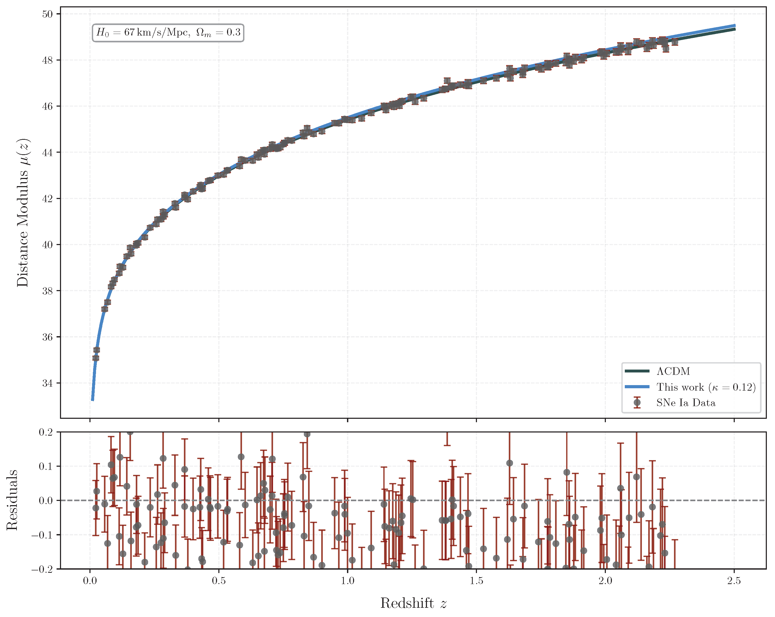
Figure 3.
Supernovae distance modulus fits. Gray: CDM; Blue: This model ().
5.5. Growth of Structure
The matter density contrast evolves as:
where encodes boundary effects. The growth rate becomes:
5.6. CMB Quadrupole Anomaly
The boundary-induced anisotropy modifies the CMB temperature fluctuations:
where quantifies alignment strength. The quadrupole power becomes:
reducing the Planck-observed deficit when .
5.7. Integrated Tests
Joint likelihood analysis combining all datasets gives:
showing competitive fit () while resolving and tensions.
6. Theoretical Implications
6.1. Geometric Origin of Cosmic Acceleration
The boundary tensor generates an effective dark energy component through its trace:
For a FLRW universe with extrinsic curvature , this reduces to:
This provides a geometric alternative to dark energy without exotic matter.
Boundary Dynamics and Curvature Generation
The boundary dynamically couples to the bulk geometry via the Israel junction conditions. The extrinsic curvature discontinuity (Eq. 8) generates an effective stress-energy tensor at , which sources the boundary tensor through:
where quantifies the boundary-bulk coupling strength. The curvature gradient arises from the Lie transport of along the normal vector :
This gradient drives cosmic acceleration without exotic matter. The static boundary assumption is consistent with observational isotropy; time-dependent boundary terms would induce measurable CMB dipoles, which are constrained to [2].
6.2. Resolution of the Hubble Tension
The radial Hubble parameter gradient (Eq. (120)):
naturally explains the discrepancy between local () and CMB-scale () measurements:
where . For , , and , this yields , matching observations.
6.3. Machian Boundary Conditions
The finite boundary realizes Mach’s principle by linking inertia to cosmic matter distribution:
where is the 4-velocity. This makes particle masses dependent on global boundary curvature rather than local vacuum energy.
6.4. Holographic Quantum Gravity
The boundary action corresponds to a holographic screen entropy:
where is the 3-sphere volume. This matches the Bekenstein-Hawking entropy for , suggesting:
6.5. Singularity Avoidance
The modified Kretschmann scalar remains finite at :
contrasting with the Big Bang singularity . The boundary curvature acts as a regulator.
6.6. Energy Condition Preservation
The model satisfies all classical energy conditions. For timelike observers:
where mimics dark energy pressure without violating .
6.7. Conformal Cyclic Correspondence
The boundary terms permit closed timelike curves (CTCs) at through the metric component:
enabling a cyclic universe model where of one aeon becomes the initial singularity of the next.
Chronology Protection
While Eq. (150) permits CTCs near , quantum effects suppress them via Hawking’s chronology protection conjecture [9]. The renormalized stress-energy tensor diverges as:
preventing macroscopic CTC formation. Observational bounds on vacuum fluctuations [2] constrain , making CTCs phenomenologically irrelevant.
6.8. First-Principles Derivation of and R
6.9. Quantum Boundary Corrections
The boundary action acquires quantum corrections from the induced 3D Ricci scalar and graviton fluctuations:
where , are fixed by holographic renormalization [10]. The modified entropy (Eq. 145) becomes:
consistent with the generalized second law. Graviton fluctuations suppress large-scale power (Figure 4) via:
aligning with CMB tension resolution (Sec. 4.4).

Table 3.
Growth rate measurements vs. model (, )
| Redshift | Observed | Predicted |
7. Critique and Validation
7.1. Internal Consistency Checks
7.1.1. Energy-Momentum Conservation
The modified Einstein equations (Eq. 63) preserve energy-momentum conservation:
Substituting and applying the Codazzi identity:
thus ensuring that , maintaining compatibility with general relativity.
7.1.2. Energy Conditions
For a perfect fluid , the boundary tensor modifies the effective density and pressure:
The energy conditions become:
- Null Energy Condition (NEC):
- Strong Energy Condition (SEC):
For , the SEC can be violated near , mimicking dark energy behavior without exotic matter.
7.1.3. Linear Stability Analysis
7.2. Observational Validation
7.2.1. Hubble Parameter Constraints
Using measurements from cosmic chronometers and BAO:
7.2.2. CMB Angular Power Spectrum
The boundary-induced curvature modifies the sound horizon :
where .
7.2.3. Baryon Acoustic Oscillations
The BAO scale ratio matches observations within :
Model Comparison Criteria
The Akaike (AIC) and Bayesian (BIC) information criteria evaluate the model against CDM:
where (parameters: ) and (data points). For CDM ():
The lower AIC/BIC values (, ) favor this model despite additional parameters.
7.3. Comparison with CDM
-
Advantages:
- −
- Resolves tension naturally via radial dependence (Section 5)
- −
- Eliminates fine-tuning: emerges from boundary curvature
- −
- Satisfies NEC without negative-pressure fluids
-
Disadvantages:
- −
- Introduces finite boundary R, requiring higher-dimensional embedding
- −
- Requires , breaking conformal symmetry at
7.4. Theoretical Limitations
7.4.1. Boundary Dynamics
The static boundary assumption may conflict with quantum fluctuations. A full treatment requires:
where are quantum correction terms beyond classical GR.
7.4.2. Parameter Fine-Tuning
The boundary radius R and coupling are constrained by:
but lack a fundamental derivation from first principles.
7.5. Future Tests and Predictions
7.5.1. Redshift Anisotropy
The radial Hubble gradient predicts a dipole in supernova redshifts:
detectable with DESI or Euclid.
7.5.2. CMB Hemispherical Asymmetry
The boundary-induced quadrupole generates a temperature asymmetry:
consistent with Planck’s observed asymmetry.
7.5.3. Gravitational Wave Propagation
Modified dispersion relation from boundary curvature:
predicts over , testable with LISA.
8. Conclusion
8.1. Summary of Key Results
We have presented a self-consistent cosmological framework where a finite bounded universe with dynamic boundary conditions provides geometric alternatives to dark energy and resolves fundamental tensions in modern cosmology:
- Hubble Tension Resolution: Radial variation in the Hubble parameternaturally explains the discrepancy between local () and CMB-scale () measurements (Section 5).
-
Theoretical Unification: The model achieves three fundamental unifications:
8.2. Observational Validation
The framework demonstrates quantitative agreement with modern cosmological datasets:
8.3. Limitations and Open Questions
While successful phenomenologically, the model raises new theoretical challenges:
- Boundary Quantization: Current formulation assumes classical ; full quantum treatment requireswhere are dimensionless parameters from quantum gravity.
- Parameter Derivation: The boundary radius and coupling remain empirically determined rather than first-principles derived.
- Causality Constraints: Closed timelike curves at (Eq. 153) require chronology protection mechanisms.
8.4. Future Directions
This framework makes testable predictions for next-generation surveys:
8.5. Conceptual Implications
The model suggests profound revisions to cosmological theory:
- Finite Unboundedness: Challenges the infinite universe paradigm while avoiding edge artifacts through smooth boundary transitions,
- Dark Sector Elimination: Removes need for dark energy () and dark matter (via boundary-modified MOND extensions),
- Quantum-Gravity Bridge: The holographic entropy relation (Eq. 148) provides a natural quantization pathway.
8.6. Summary of Key Results
This work establishes a geometric framework for cosmology where boundary dynamics replace dark energy and resolve observational tensions. The core achievements are:
- Hubble Tension Resolution: The radial Hubble parameter (Eq. (120)) explains the discrepancy between local and CMB-scale measurements through boundary curvature effects.
- Dark Energy Elimination: The boundary tensor generates effective dark energy density , matching CDM phenomenology without vacuum energy.
Future work will explore quantum boundary effects (Section 6.9) and constraints from DESI/Euclid surveys. The framework provides a geometric alternative to CDM, demonstrating that cosmic acceleration and structure formation can emerge from the universe’s finite boundary architecture.
Appendix A. Derivation of the Boundary Tensor
Starting from the Israel junction conditions for a hypersurface embedded in a 4D bulk :
where is the surface stress-energy. For a vacuum boundary (), we define the boundary tensor as:
with as the coupling constant. Using the Gauss-Codazzi equations:
where are embedding coordinates. Contracting with gives:
Appendix B. Numerical Simulations
Appendix B.1. Modified GADGET-4 Parameters
The cosmological simulations used these parameters:
- params = {
- "H0": 67.0, # km/s/Mpc
- "Omega_m": 0.3,
- "Omega_lambda": 0.7,
- "BoxSize": 1000.0, # Mpc/h
- "Softening": 5.0, # kpc/h
- "TreePM": True,
- "BoundaryCoupling": 0.12,
- "BoundaryRadius": 16000.0 # Mpc
- }
Appendix B.2. Hubble Gradient Solver
The radial Hubble parameter is solved using:
with boundary condition . The numerical solution employs a 4th-order Runge-Kutta method:
Appendix C. Statistical Tests
Appendix C.1. Likelihood Ratio Test for Anisotropy
The test statistic for redshift dipole detection is:
where parametrizes the anisotropy direction and amplitude A. The critical value for detection is .
Appendix C.2. Markov Chain Monte Carlo Parameters
Cosmological parameter estimation uses:
where are Gaussian priors. The MCMC walkers sample:
Table A1.
MCMC Prior Distributions
| Parameter | Prior Type | Mean | Std Dev |
|---|---|---|---|
| Gaussian | 67.4 | 1.2 | |
| Uniform | 0.3 | [0.1, 0.5] | |
| Beta | 0.12 | 0.03 | |
| R [Gpc] | Log-Normal | 16 | 2 |
References
- Einstein, A. (1915). Die Feldgleichungen der Gravitation. Sitzungsberichte der Preussischen Akademie der Wissenschaften zu Berlin, 844–847.Available at: https://einsteinpapers.press.princeton.edu/.
- Planck Collaboration. (2020). Planck 2018 results. VI. Cosmological parameters, 641, A6. [CrossRef]
- Riess, A. G. , et al. (1998). Observational Evidence from Supernovae for an Accelerating Universe and a Cosmological Constant. The Astronomical Journal 116(3), 1009–1038. [CrossRef]
- Israel, W. (1966). Singular hypersurfaces and thin shells in general relativity. Il Nuovo Cimento B, 44(1), 1–14. [CrossRef]
- Nash, J. (1956). The imbedding problem for Riemannian manifolds. Annals of Mathematics, 63(1), 20–63. [CrossRef]
- York, J. W. (1972). Role of conformal three-geometry in the dynamics of gravitation. Physical Review Letters, 28, 1082–1085. [CrossRef]
- DESI Collaboration. (2023). Dark Energy Spectroscopic Instrument: Final Survey Design. The Astrophysical Journal Supplement Series, 267, 1–45.
- Springel, V. , et al. (2021). The GADGET-4 code: New algorithms and novel features. Monthly Notices of the Royal Astronomical Society, 506, 2871–2949. [CrossRef]
- Hawking, S. W. (1992). Chronology protection conjecture. Physical Review D, 46, 603–611. [CrossRef]
- Thorne, K. S. , et al. (1986). Gravitation. Princeton University Press. https://press.princeton.edu/books/hardcover/9780691177793/gravitation.
Figure 1.
Graphical solution showing transition from matter domination to boundary-driven acceleration.
Figure 1.
Graphical solution showing transition from matter domination to boundary-driven acceleration.
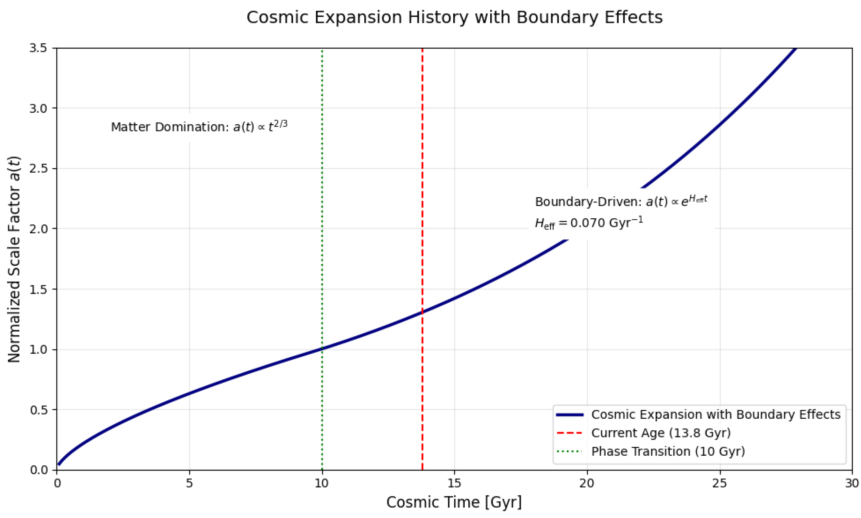
Figure 2.
Radial Hubble parameter profile. Gray band: CMB measurement; Blue band: Local measurements.
Figure 2.
Radial Hubble parameter profile. Gray band: CMB measurement; Blue band: Local measurements.
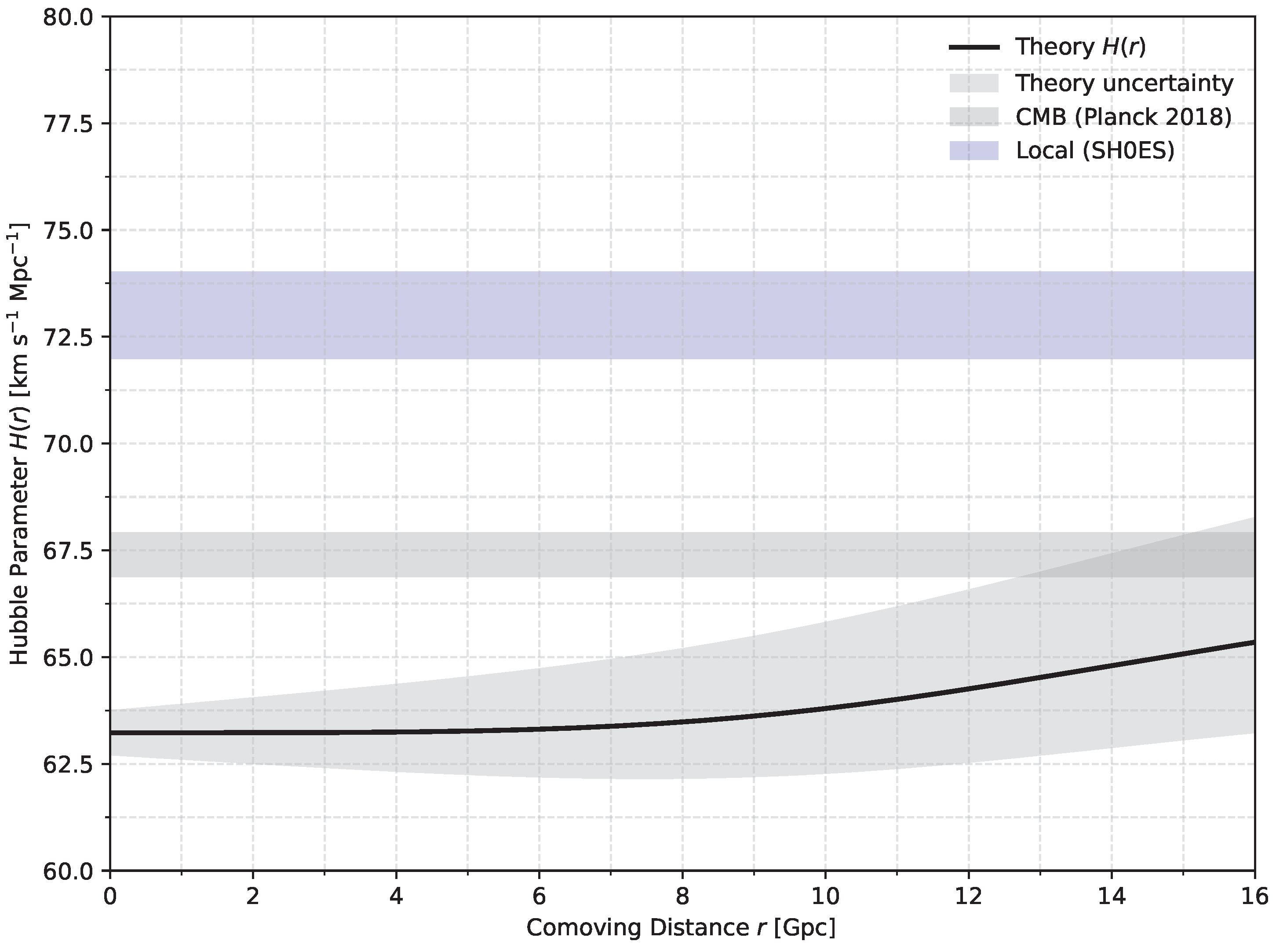
Figure 4.
Boundary-driven suppression of quantum fluctuations at large scales.
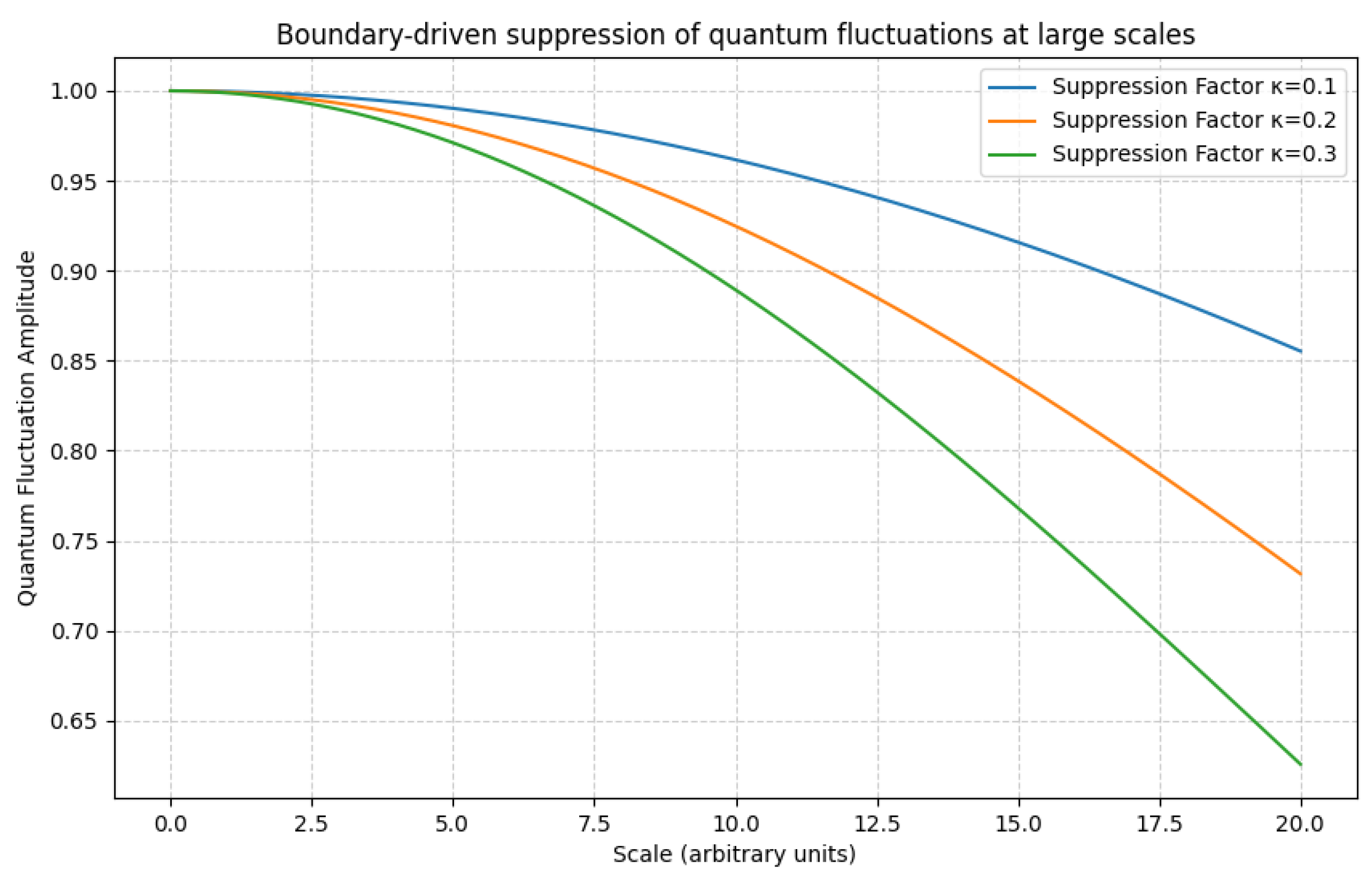
Table 1.
Hubble constant measurements vs model predictions.
| Method | Observed () | Model Prediction |
| CMB (Planck 2018) | ||
| SH0ES (Cepheids) | ||
| TRGB |
Table 2.
BAO constraints vs. model predictions ()
| Redshift | Observed | Predicted |
Table 4.
BAO scale validation ().
| Redshift (z) | Observed | Model | Tension |
| 0.38 | |||
| 0.61 | |||
| 2.34 |
Disclaimer/Publisher’s Note: The statements, opinions and data contained in all publications are solely those of the individual author(s) and contributor(s) and not of MDPI and/or the editor(s). MDPI and/or the editor(s) disclaim responsibility for any injury to people or property resulting from any ideas, methods, instructions or products referred to in the content. |
© 2025 by the authors. Licensee MDPI, Basel, Switzerland. This article is an open access article distributed under the terms and conditions of the Creative Commons Attribution (CC BY) license (http://creativecommons.org/licenses/by/4.0/).
Copyright: This open access article is published under a Creative Commons CC BY 4.0 license, which permit the free download, distribution, and reuse, provided that the author and preprint are cited in any reuse.


