
Submitted:
31 January 2025
Posted:
03 February 2025
You are already at the latest version
Abstract
Understanding lagoon behavior is crucial for both scientific research and engineering, especially in delicate Arctic environments. Lagoons are vital to coastal areas, often bol-stering infrastructure resilience. Since Spring 2019, we've monitored the Longyearbyen lagoon (Spitsbergen), vital for coastal erosion defense and serving as a natural laboratory. The location's well-developed infrastructure and accessible logistics make it an ideal testing site available at any time. It can be used for many natural scientific studies.
Spanning 400x50m, the lagoon continually shifts due to waves and tides, with a maximum tidal range of 2m. This article focuses on gravel spit movement, accelerating in recent years to several meters monthly. Through methods like aerial and satellite images, laser scanning and hydrodynamic measurements, we've delineated processes, rates, and mechanisms behind this movement. Bed-load transport along the spit, coupled with gravel slides, primarily drives expansion and lagoon growth. Modeling these processes aids in forecasting lagoon system development, crucial for informed management and engineering decisions in Arctic coastal regions.
Keywords:
Spitsbergen
; lagoon
; gravel spit
; bed-load transport
; tide
; coastal dynamics
; laser scanning
1. Introduction
Lagoon definition, spreading and studies
Coastal lagoons are bodies of water that are partially isolated from an adjacent sea by a sedimentary barrier, but which nevertheless receive an influx of water from that sea. Some 13% of the world's coastline is associated with lagoons [1]. Lagoons do not receive a large freshwater inflow in contrast with estuaries. One may distinguish between microtidal and macrotidal lagoons, open and closed lagoons and intermediate state.
Due to rocky coast, lagoons are not so largely presented in the Arctic. Nevertheless, several lagoons became test sites and known in scientific community.
For example, Kaktovik Lagoon (Beaufort Sea) was one of the study sites for the National Science Foundation's Beaufort Lagoon Ecosystems LTER program in 2018-2019 with main focus on the discontinuities of pH variability and CO2 flux at the air–sea interface [2]. Electrical geophysics revealed the absence of ice-bonded permafrost beneath this lagoon [3]. Three lagoons in Kotzebu Sound (Chukchi Sea, Alaska) gave valuable information about energy flow and trophic dynamics in Arctic ecosystem [4]. Thermokarst processes were investigated in five lagoons of Bykovsky Peninsula (Laptev Sea) [5]. Valkarkai Lagoon is known by long sea level and meteorological data series (1956-1993) on remote Chukchi Sea coast [6]. The Vallunden Lagoon in the Van Mijenfjorden (Spitsbergen) was used many times for fields works at UNIS (see, e.g., [7-9]. Research programs at most of the above-mentioned sites are mostly oriented on biology, geochemistry and the sea ice processes and do not touch spit movement.
Despite their limited global distribution, lagoons are of significant interest to coastal processes in the Arctic, especially in the context of global warming [10-12].
Very relevant and important the local investigations, devoted to spit morphodynamics and showcasing how the global warming trend accelerates coastal geomorphic changes at the head of the deglaciated fjords [13-19]. Strzelecki and coauthors in [15] detailed the post-Little Ice Age (LIA) (1590–1850 AD) sediment fluxes to the coastal zone in Billefjorden, central Spitsbergen(Svalbard) and analysed the response of the gravel-dominated barrier coast to the decay of Ferdinandbreen. They showed that glacier retreat resulted in the development of paraglacial sediment cascade where eroded and reworked glacigenic sediments progressed through alluvial fans to the coast, thus feeding gravel-dominated spit systems in Petuniabukta. The acceleration of coastal erosion and associated spit development was coincident with rapid climate warming from the 1980s. In colder phases of post-LIA period, coastal zone development was subdued and strongly dependent on the efficiency of sediment transport via in a longshore drift. Kim and coauthors [13] on the base of repeated photogrammetry survey (2016-2019) found that gravel spit complexes on the tidal delta plain at the head of Dicksonfjorden (Northern branch of Isfjorden) display pronounced morphodynamic variability in time and space. The youngest spits elongated 22 m/yr and migrated landward 4.3 m/yr. The spit morphodynamics here is driven primarily by longshore drift and to a lesser degree by overwash processes.
We add to these investigations of lagoon development the precise laser scanning measurements and hydrology studies, uncovering the physical mechanism of spit movement.
Inventory, provided by Norwegian Polar institute in 2016 [20], estimates the presents of Lagoons and Barrier Islands together with Estuaries as 29% of Svalbard coastscapes. But Longyearbyen lagoon is not presented in the Inventory because of small size. We investigate Longyearbyen lagoon as important site for local community/infrastructure and scientific experiments.
Longyearbyen Lagoon. Environment. Morphometry. Development
Investigated lagoon is in the High Arctic (coordinates DD MM SS: 78°13′25″N 15°40′11″E) in Adventfjorden, near Longyearbyen (Figure 1), the biggest settlement of Spitsbergen. Longyearbyen with only two and half thousand citizens became famous as a tourist destination and the test site or start point for many Arctic studies due to its developed infrastructure and transport accessibility. Marine environment of Adventfjorden is detailly studied and described in the booklet [21]. In the same sense, Longyearbyen lagoon is remarkably interesting for investigation of coastal process and conducting various full-scall experiment in natural conditions. Coastal processes are particularly important in Arctic region with permafrost spreading on the background on ongoing climate change [22]. The consequences are visible and convenient to investigate in Longyearbyen, where warming up 7 times faster than the whole planet warming was reported [23, 24]. The lagoon is only 600 m to walk from the Svalbard Science Park, including the University Centre in Svalbard (UNIS), Norwegian Polar Institute and other research organizations (Figure 2).
It is only 600 m to walk from the Svalbard Science Park, including the University Centre in Svalbard (UNIS), Norwegian Polar Institute and other research organizations (Figure 2).
The lagoon was formed and developed under the influence of sediment transport from the Longyear River, currents, and tidal processes. During the snowmelt period, a significant volume of sediment from surrounding slopes and glacial erosion is carried to the fjord and redistributed by the water motion in Adventfjorden. The sediments predominantly consist of local bedrocks such as sandstones and shale, with occasional inclusion of magmatic stones brought from the mainland for riverbed reinforcement [27]. The lagoon spit is composed of gravel, with varying proportions of sand, granules, and pebbles of different sizes and roundness (see the corresponding section of Result chapter).
Sediment amount and regime depends on local weather and climate and increased significantly last years while global warming is the most pronounced in the Arctic and particularly in Longyearbyen [28-32]. That arise questions on risk and city sustainability, and push the preventive measure [33, 34]. The Longyear River has been artificially channeled to create space for the settlement, and periodic efforts are made to enhance its bed and adjacent slopes. These alterations have led to a more controlled sediment flow regime [32, 35, 36].
A sewer pipe running through the central part of the lagoon disrupts natural processes. The pipe (shown by the purple arrow in Figure 2) is buried to a shallow depth and becomes visible, surrounded by sediment accumulation, at low tide in the fjord behind the spit (Figure 5). Currently, the influx of fresh water from the Longyearbyen River is minimal, since the main flow is directed directly into the fjord. Despite this, the lagoon remains largely open to the fjord, and the salinity level of the water matches that of the fjord.
The location of the lagoon in the southeastern internal region of Adventfjorden dictates the tidal and wave patterns it experiences. In the Longyearbyen/Adventfjorden area, the maximum tidal range measures 2.1 meters, while the minimum range ranges from 0.33 meters at its lowest to 0.82 to 1.17 meters at its highest. Figure 3 illustrates the typical tidal fluctuations in Longyearbyen. Adventfjorden, a relatively small eastern branch of the expansive Isfjorden, opens widely into the Greenland Sea. Within the Isfjorden, the M2 tide holds sway with a period of 12.42 hours [37]. The maximum speeds of tidal currents are contingent upon local topography, ranging from 2 to 10 centimeters per second in broader expanses to several meters per second in the narrow straits of Spitsbergen fjords [38]. Notably, the more vigorous currents are often confined to shallow passages, such as at the entrance to the Dicksonfjorden (the northern branch of Isfjorden) and in the central sector of the Van Keulenfjorden (another fjord opening into the Greenland Sea).
Due to its geographical positioning, the greatest wave fetch occurs at the entrance to Adventfjorden from Isfjorden, particularly in the Vestpynten area. Direct measurements using Acoustic Doppler Current Profilers (ADCP) indicate that maximum wave heights in this area typically remain below 1.5 meters [40]. Towards the end of Adventfjorden, wave heights diminish considerably as they dissipate in shallower waters. Nonetheless, even in these shallower regions, waves may still play a role in sediment transportation. Of paramount importance here is the velocity of water movement, which we have meticulously measured to unravel the mechanisms behind gravel spit migration.
While Adventfjorden has been predominantly ice-free in recent years, ice typically persists in the lagoon from November through May due to the comparatively tranquil water movement. Winds originating from the East tend to push ice into the lagoon, contrasting with Adventfjorden where wind influences ice drift out of the fjord. The drag exerted by West winds, accumulating over several hundred meters of the lagoon, is insufficient to break up ice within the lagoon. During low tide, ice on the lagoon surface can bend by up to 80 centimeters. The mouth of the lagoon represents the most dynamic area, characterized by significant bending, periodic ice breaking, and floe movement, leading to erosion [41].
Ice floes, measuring up to 0.9-1 meter in thickness, can be also transported from Adventfjorden to the lagoon area, where they become stranded north of the spit. These floes originate locally and represent calved pieces of the ice foot—a belt of ice frozen to the shore, primarily formed due to tidal fluctuations—and can accumulate near the beach, forming rubble. Larger floes and small icebergs originating from Isfjorden [42] do not reach the lagoon area, as they become stranded in the shallow waters to the west.
In certain years, such as those before 2009 and notably in 2024, Adventfjorden has been completely covered by ice, resulting in the appearance of small shore rubble on the spit beach. Beneath this ice cover, the velocity of tidal water motion escalates. This intriguing ice phenomenon in the region warrants further investigation, particularly since spit movement is not solely confined to warmer periods, when sediment influx from the river is most vigorous and coastal relief reshaping would be more expected and evident. Through our observations of the lagoon, we have determined that at times during winter, the gravel spit can migrate eastward, sometimes even more prominently than during summer months. This underscores the complexity of the mechanisms driving spit movement and highlights the need for comprehensive research into the interplay between ice dynamics and coastal geomorphology.
Tidal fluctuations, ocean currents, and sediment deposition from rivers collectively influence the dynamic shape of the lagoon and the shifting position of the spit. Primarily, the head of the spit steadily advances eastward, towards the inner reaches of Adventfjorden, starting from the mouth of the Longyear River. Since our observation commenced in 2019, the spit has migrated eastward by over 200 meters and protruded approximately 400 meters from its original location, a transformation evident on all conventional maps of Longyearbyen (Figure 2).
2. Materials and Methods
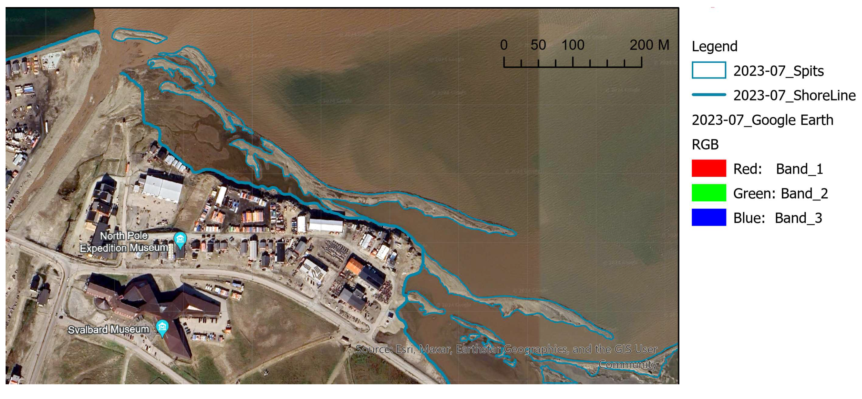
A comprehensive array of measurements has been conducted since 2019 to characterize and elucidate the movement of the lagoon spit. Figure 4 delineates the locations of equipment and measurement positions. To accurately represent the changing contours and form of the lagoon spit, we have depicted its morphology during the field campaigns in Autumn 2022 and 2023, by red and blue lines over readily accessible satellite imagery from Google Earth, reflecting the state of July 2023 [25], that serves as a base layer in Figure 4. This depiction serves as valuable visual aids in capturing the dynamic evolution of the lagoon spit over time and measured parameters (see the Results section).
Aerial photos and satellite images
A compilation of aerial photographs and satellite images showcasing the evolution of the lagoon has been integrated using ArcGIS Pro software. Georeferenced images from the years 1936 [43], 2009 [26], 2021 [44] and 2023 [25] enabled the digitization of the coastal line and lagoon spit into polygons (Figure 15). These images, along with their digitized representations, are shown in Appendix 1.
Additionally, data from [41] was utilized to reconstruct spit movement using aerial photographs since 2005. According to this data, the end of the lagoon spit has shifted 300 meters eastward over a span of 15 years (2005-2019), indicating an approximate rate of 20 meters per year. This historical perspective provides valuable insight into the ongoing dynamics of spit migration in the lagoon.
Laser Scanning
Since 2019 we follow lagoon spit advancing by laser scanning with Riegl VZ1000. Riegl VZ1000 is Terrestrial Laser scanner with accuracy 8 mm and precision 5 mm. An efficient measurement rate up to 122,000 measurements/sec. Maximum range of 1400 m at 70 kHz. It makes point cloud on a distance up to one km [45].
During the ice-free season, the bottom of the lagoon is exposed at low tide, revealing wet clay deposits on the surface or shallow waters in both the internal and external parts of the lagoon. This unique feature enables the topography of the gravel spit to be accurately reflected through 3D point cloud technology and visualized following processing. Capturing the lowest water level, which occurs only several times per year, is crucial for this purpose.
To achieve this, we conducted 13 laser scanning sessions from a wooden terrace near the so-called bird observation house (blue construction in Figure 5), situated 10 meters above the lagoon. This vantage point facilitated the rapid reflection of the lagoon and spit surface. Figure 5 illustrates the laser scanning procedure and depicts the appearance of the lagoon during low tide on October 1, 2023. However, the spit slope facing the fjord was not visible from this position. To address this limitation, we conducted measurements from scan positions directly on the spit itself, twice in September 2022 and October 2023 (refer to scan positions in Figure 4 – orange and green circles). This approach enabled us to meticulously map the topography of the spit, providing detailed insights into its morphology and spatial characteristics.
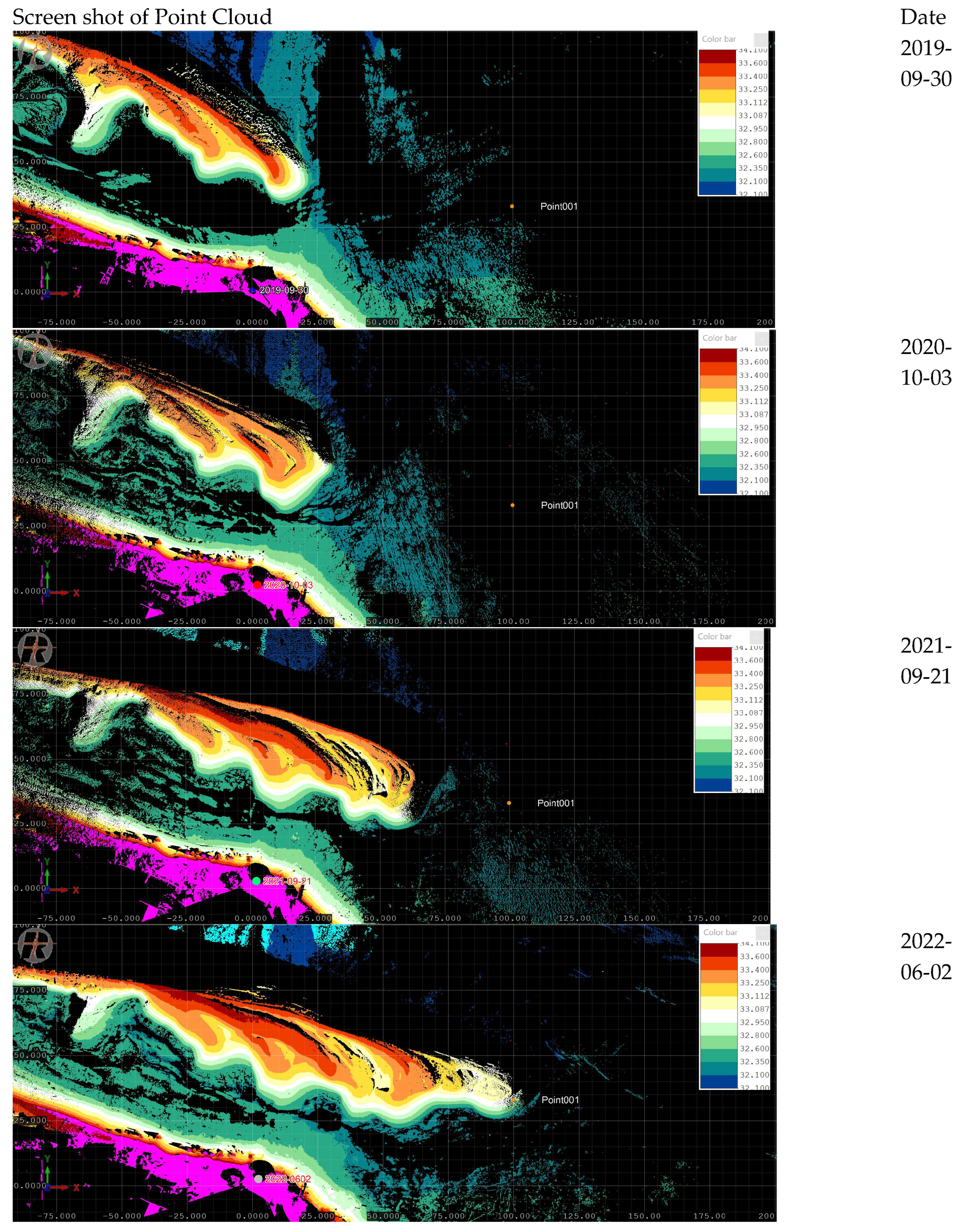
The RiScan Pro software [46] was employed for the initial processing of raw scans, which involved accurate adjustments, filtering, visualization, and export to common 3D formats. Figure 6 provides an illustration of the program interface and the resulting data, showcasing point clouds for specific days and times. This software facilitated efficient processing and analysis of the scan data, enabling us to derive valuable insights into the morphology and dynamics of the lagoon and spit. The visualization in Figure 6 reveals the evolving topography of the gravel spits as captured in 2019 and 2023. The presented view from above with coordinate axes in meters with a palette in traditional topographic colors shows the height of gravel spits of about 2 meters (from 32.1 to 34.2 in the project coordinate system, which corresponds to WGS84 Ellipsoid Height) and the advance of the ridge of the spit (red-cinnamon color) by 180 meters to the east in 4 years. This gives an idea of the possibilities that scanning data processing provides for monitoring the movement of streamers. By successively opening and digitizing the point clouds obtained during scanning, we tracked the movement of streamers over 4 years, as shown in Figure 15 for eight key scans.
Hydrodynamic measurements
Hydrodynamic measurements included measurements of tidal variations of sea water and ground water levels in the spit, and measurements of sea current velocities near the spit. See location of instruments in Figure 4. Measurements of sea water and ground water levels were performed with 3 pressure and temperature recorders SBE 39 Plus (SBE1, SBE2, and SBE3) with sampling interval of 1 minute [47]. Sensor SBE1 was installed inside plastic pipe (test pipe) with diameter 10 cm placed in the spit on the depth 1.5 m (7,8). The pressure sensor measured ground water pressure at the bottom of the pipe. Place of measurements is marked by PS in Figure 7. The pipe was protected on the top from rainwater (Figure 8a). Small holes in the lateral surface of the pipe were made to support atmospheric pressure inside the pipe above the water. The pipe was installed near the spit tip on October 10, 2022 (Figure 8b). The second sensor SBE 2 was mounted on the leg of metal frame used for the installation of the acoustic Doppler velocimeter ADV, SonTek Ocean Probe 5 MHz (Figure 9a). The length of frame near the bottom was 60 cm (Figure 9b). The third sensor SBE3 was deployed at the sea bottom on the depth of about 10 m in Longyearbyen harbour on 1 km distance from SBE1.
All sensors were deployed from the same computer with UTC time setting. The records were synchronised in time. Dates of sensor deployments are given in Table 1.
Sediment samples
Sediment samples were collected in four places of gravel spit to characterize the sediment composition (Figure 11, Figure 12 and Figure 13). The samples characterize the essentially different positions in relief and condition of sediment transport. Point 1 is the tip of the gravel spit, the most advanced part where forward movement occurs. Point 2 is a shallow plain near the spit, exposed from the water only at low tide, where an accumulation of fine sediments is visible. Similar conditions exist in the interior of the lagoon and at the bottom of the fjord with calm water. However, it was interesting to show the contrast between the dynamic tip and the calmer shallow water, locating only in several meters from each other. Points 3 and 4 are in the middle, already formed part of the gravel spit, on the ridge (not flooded at high tide) and on the beach (covered by water in high tide and constantly being under the influence of waves/currents), respectively. It should be noted that even this middle part of spit can change its position, moving mainly towards the shore, as can be seen when analysing photo images from previous years and laser scanning results. That is, it is also very dynamic.
Figure 12 and Figure 13visualize the samples. They were processed following the traditional sediment analysis protocol [48]. We use the set of sieves – 1/16, 1,2, 4, 6.3, 8.10 and 20 mm to get the diagram (Figure 16). The shallow sample significantly changed after treatment, and it is shown on Figure 12c. Initially wet silt sludge sample had formed upon drying into clots 1 to 3 cm in size, looked like stones (Figure 12b). These clots turned into fine dust after sifting (Figure 12c). The organic residues reviled as black sticks about 1-2 mm in size (Figure 12c bottom right corner).
Figure.13 Sediment samples from the middle part of the spit. (a) - Sample 3. From the ridge of the spit; (b) - Sample 4. From the spit beach
3. Results
3.1. Longyearbyen lagoon system development 1936-2023
Reconstruction based on georeferenced images (Figure 14) reveals the dynamic and ever-changing nature of the lagoon system. These changes are depicted in Figure 14 by the shoreline and spit contours represented as polygons, with colors corresponding to different years. Original images and their digitalization are presented in Appendix 1. There have always been several spits stretching from the Longyear river in an east-east-south direction. This natural phenomenon is typical of coastal environments where gravel spits often develop due to significant wave action and longshore drift. Wind and water currents play a crucial role in shaping these spits, contributing to their elongation or curvature depending on their direction.
In the 1936 image, prior to significant anthropogenic influence, one relatively straight and thin spit is observed with a hook formation near the river, while several spits with thickenings at the base of curved (hook) ends can be seen half a kilometer to the east. By the year 2009, the coastline underwent transformation due to the construction of an embankment, replacing former sandbanks with structures. This embankment cast a shadow over the eastern system of spits, while three short spits near the delta (left part of the image) curved towards the shore in a south-southeast direction, a configuration now commonly depicted on maps of Longyearbyen. In the 2021 image, both the gravel spit in the shadow of the embankment and the spits along the coastline had significantly shifted eastward (by 230 and 140 meters respectively) and assumed an east-east-south direction. Those nearer to the delta exhibited a pronounced bend towards the south, whereas the eastern ones expanded more towards their ends. By 2023, the imagery depicted four short gravel spits near the delta, a substantial advancement and approach of the central spit towards the shore, moving eastward by 112 meters. Consequently, the access of fresh water to the central lagoon has ceased, while the spits sheltered by the embankment remained relatively unchanged.
3.2. Spit expansion rate 2019-2023
Based on laser scanning data, we can provide a detailed estimation of the speed of gravel spit expansion. Figure 15 illustrates the locations of spit ends at the time of scanning, with each day of measurements highlighted by arrows. This visualization allows for a precise tracking of the spit's growth over time.
The movement of the gravel spit over a span of four years is depicted through the presentation of 10 cm thick slices from the point clouds in the upper part of the spit, each marked with different colors corresponding to the days of measurements. Red arrows indicate the easternmost positions/ends of the spit as per autumn surveys. Notably, the spit exhibited rather insignificant movement, shifting 8 meters eastward from September 30, 2019, to October 3, 2020. Subsequently, in the following year (2020-2021), it advanced by 40 meters, and a further 42 meters from autumn 2021 to autumn 2022. Accelerating its pace, the movement doubled the following year, covering 86 meters from September 11, 2022, to October 5, 2023.
Intermediate shots marked by green arrows reveal interesting trends. For instance, during the 8 winter months from September 2021 to June 2022, the movement was notably subdued, totaling 18 meters, compared to the 24 meters recorded over the 4 warm months from June to September 2022. Noteworthy is the movement during the winter of 2023, where it exhibited remarkable activity. Specifically, from September 2022 to February 2023, the spit moved 40 meters, followed by 19 meters from February to June 2023, and a further 27 meters from June to October. The trend persisted, with the spit moving an additional 30 meters eastward from October 2023 to February 2024, according to GPS measurements.
3.3. Results of hydrodynamic measurements
Blue and green lines in Figure 16a show respectively sea water levels measured by SBE3 and SBE2 versus time. Blue lines were moved in the vertical direction to offset zero mean seawater level. Blue line wase moved in the vertical direction to get zero mean level of seawater. Green line was aligned by upper level of seawater since water levels measured by SBE2 and SBE3 should coincide by high tide. Green and blue lines are almost coinciding. The local minima of blue line are slightly below the local minima of green line since sensor SBE2 was above sea level in low tide. Green lines in Figure 16a,b are the same. Yellow line in Figure 16b shows ground water level measured by SBE1 versus time. Yellow line was aligned by upper level of seawater measured by SBE2. Local minima of yellow line are above local minima of green line because the location of ground water measurement by SBE1 (point PS in Figure 7) was above the location of pressure measurement by SBE2 (point PS on SBE2 in Figure 9a). Increasing thickness of green line in Figure 16 is explained by the influence of surface waves during storm weather when .
Blue and yellow lines in Figure 17a show respectively sea water level measured by SBE3 and ground water level measured by SBE1 versus time from October 12, 2022, to June 17, 2023. Yellow line was aligned by upper level of seawater measured by SBE3. Maximal difference between ground water and sea water levels reached in low tide was about 0.5 m. Zoomed fragment of the dependences shown in Figure 17b corresponding to the last syzygy tide in January 2023 shows good correlation in time between the local maxima of seawater and ground water levels demonstrating relatively high permeability of the spit soil. Ground water levels began to increase immediately after seawater and ground water levels became equal after low tide.
Results of ADV measurements are shown in Figure 18, Figure 19 and Figure 20. Figure 18a shows mean water speed in each burst versus time measured at the distance 15 cm from seabed in location ADV-I. Figure 19b shows mean water speed in each burst versus time measured at the distance 10 cm from seabed in locations ADV-II and ADV-III. Figure 19a shows the time intervals when ADV was covered by the water and measured water pressure and water velocity. Measurements were not performed in low tide when ADV was above the water level. All ADV velocity data shown in Figure 18-20 are of a good quality. Blue points in Figure 18b and Figure 20 have coordinates of East and North water velocities measured with 10 Hz sampling frequency. Yellow points in Figure 19b and Figure 20 have coordinates of mean East and North water velocities in each burst.
Figure 18b shows that mean and wave induced water motions in location ADV-I were almost reciprocating directed from North-West to South-East. Fi Figure 20a indicates that mean water motion was almost reciprocating in location ADV-II of the same direction, but wave induced water motions occurred in directions from North-West to South-East, and from North to South. It is explained by the interaction of waves near the spit tip. Figure 20b shows reciprocal mean motion of the water along the spit in Location ADV-III, and wave induced motion from North-West to South-East. Maximal mean speed of water reached 30 cm/s in Locations ADV-I and ADV-II. Water speeds measured in location ADV-III were lower 10 cm/s.
Standard deviation of water speed was calculated in each burst with the formula
where and are standard deviations of East () and North () velocities measured with 10 Hz sampling frequency. Standard deviation characterises wave amplitudes. Horizontal Reynolds stresses near seabed were calculated in each burst with the formula
where symbol
means averaging over 2 min, , , and are the fluctuations of water velocities. Standard deviations of water speed and Reynolds stresses are shown versus time in Figures 18c,d for measurement location ADV-I and in Figures 19c,d for measurement locations ADV-II and ADV-III.
Spectral analysis showed dominating wave frequencies in the range 0.2-0.4 Hz in all locations. Higher wave frequencies up to 1 Hz were also found in some bursts. Swell frequency of 0.1 Hz was found in few bursts. Swell amplitudes were smaller amplitudes of local wind waves. Figure 18c and 19c indicate wave induced water velocity amplitudes below 30 cm/s, 20 cm/s, and 10 cm/s respectively in locations ADV-I, ADV-II, and ADCV-III.
Blue points in Figure 18b shows dominant direction of wave propagation from North-West to South-East under the angle of about 30o to the North from marine side of the Adventfjorden in location ADV-I. Not narrow cloud of blue points indicates the waves of other directions. Dominant direction of wave propagation is similar the direction of mean current in this point.
Figure 18dandFigure 19dshow that Reynolds stresses are well correlated with standard deviations of water velocities indicating wave amplitudes. Maximal Reynolds stresses reached and exceeded 3 N/m3 in location ADV-I. In location ADV-II maximal Reynolds stresses were below 2.5 N/m2, but time of measurements was much shorter than in location ADV-I. In location ADV-III Reynolds stresses were below 0.75 N/m2. Reynolds stresses are used further to estimate stability of gravel with the Shields formula.
Blue points in Figure 20a show that wave system included waves of South-East and South directions near the spit tip in locations ADV-II. In location ADV-III waves propagated from South-East to Nort-West from the lagoon to inner side of the spit. Location ADV-III was in wave shadow zone of waves propagating from the fjord behind of the spit.
3.4. Sediment analysis
As depicted in Figure 12 and Figure 13, the composition of the lagoon spit primarily comprises local bedrocks, predominantly coarse- and fine-grained sandstones (appearing grey or brown) and shale (appearing almost black due to dark clay), with occasional inclusions of magmatic stone (displaying red, white, or grey hues). The larger pieces typically consist of sandstone, which exhibits greater resistance to erosion. These rocks generally range from sub-rounded to well-rounded in shape, with occasional sub-angular pieces. The size spectrum varies from silt to pebble, occasionally including small cobbles of differing roundness in varying proportions.
Utilizing the traditional Wentworth grain size scale [49], we can further characterize the composition of the gravel spit as follows:
The slope of the spit tip (Sample 1 in Figure 12a) primarily consists of pebbles (48%), granules (27%), and sand (24%), with a negligible amount of silt (less than 1%). Moving towards the shallow plane near the tip of the spit, located just 4 meters from Point 1 (Sample 2 in Figure 12b), the composition shifts to predominantly silt (59%) and fine-grained sand (less than 1 mm) (34%), with minimal granules and rare pebbles (1%). Initially, the sample was wet, and upon drying, the silt sludge adhered together into lumps, forming clots ranging in size from 1 to 3 cm (Figure12b). Organic residues, such as small light blades of grass or sticks approximately 1 cm in size, were visible. Subsequent crushing of the lumps, removal of the silt sludge, and drying resulted in the organic residues appearing as black sticks about 1-2 mm in size, with the sediment displaying the appearance depicted in Figure 12c (bottom right corner). The organic content was determined to be 5.3% of the dry weight, and it was not factored into the granulometric composition evaluation (Figure 21).
The composition of the spit ridge (Sample 3 in Figure 13) primarily consists of pebbles (48.6%, mostly small) and sand (40.9%, with 34% being less than 1 mm), with a smaller proportion of granules (10%). Transitioning to the spit beach (Sample 4 in Figure 13), the composition shifts to mostly fine (1-2 mm) sand (58%), coarse (1-2 mm) sand (17%), granules (6%), and relatively small pebbles (14%). Occasionally, small oblong cobblestones about 7-10 cm in size are encountered on the ridge and beach, as depicted in Figure 13b in the upper right corner. These larger cobblestones were not included in the calculations for granulometric composition. Additionally, Samples 1, 3, and 4 also contain a small amount (less than 1%) of silt.
We also used previous sediment studies on the Longyearbyen coastline. Samples for grain size analysis were taken from the top 2 m layer of sediment on the shore near the spit. Initial grain size distribution curve is shown in Figure 21 by solid line. Grain diameters and are ~5.5 mm and ~23 mm. Dashed line in Figure 21 is constructed from solid line by removing of sand particles with diameters smaller 1 mm. Diameters and are ~8 mm and ~23 mm for dashed line. Further it is assumed that dashed line describes particle size distribution with gravel slope at the spit tip.
4. Discussion and Conclusion
The stability of granular material in flow can be determined by the Shields criterion [50]. The Shields approach is based on a uniform, permanent flow with a turbulence generated by the bed roughness. In our case there is additional flow pulsations generated by waves. As it is shown in [51], the Shield criterion is also valid for conditions with currents plus waves. The criterion is based on the consideration of the critical value of the Shield parameter
where is total water stress at the bed including stresses due to current and wave motion, and are the densities of soil grains and water, is the is the mean or average particle size grain diameter, and is the acceleration of gravity.
The criterion of soil stability at the bed is given by the formula
where is the particle Reynolds number, the function is approximated by thin line with in Figure 22, coefficients and characterises the influence of bottom slope in normal and parallel directions to the flow direction, and is the damage parameter changing from 0.4 by occasional particle movement to 1 by frequent particle movement. Coefficients and are estimated with the formulas
where and are the bed slope angles slope in normal and parallel directions to the flow direction, and is the angle of repose. Signs “+” and “-” are related to upsloping and down sloping motions.
Inclined lines in Figure 22 are calculated with different diameters and changing from 0.1 N/m2 to 3 N/m2. Values of water stresses correspond to calculated Reynolds stresses in Figure 18d and Figure 19d. Grain density was measured and assumed equal 2600 kg/m3. Water density equals 1000 kg/m3. One can see that grains of diameter greater 4 mm are stable at the horizontal bottom. Grains with diameters 0.5 mm, 1 mm, and 4 mm start to move when Reynolds stresses reach respectively 0.25 N/m2, 0.48 N/m2, and 3 N/m2. Thus, sand is not stable under the local conditions, but coarse gravel with grain diameters greater 5 mm is stable.
Van Rijn [51] noted that depends also on , and , where 90% of particles have diameters smaller , and is water depth. The ratio expresses the grading of the bed material. Sand particles are more difficult to mobilize when they are hiding between larger gravels. It a reduction of when 0.2. Representative value of calculated from Figure 21 equals 0.24 for soil taken from top 2 meters of the beach. Sand concentration of the spit tip is smaller. The value of reaches 0.35 on the dashed curve in Figure 21, constructed from the solid curve by the removing of particles with diameters smaller 1 mm. The value of may drop to 0.4 in this case. Figure 22 indicates mobility of gravel with diameters smaller 8 mm in this case. Thus, accumulation of gravel at the end of the spit can be explained by combined action of tidal current and waves.
and show critical values of the Shields parameter versus granular Reynolds number . Inclined lines show values of the Shields parameter calculated with Reynolds stresses changing in the range (0.1,3) N/m2. Grain diameters are pointed out.
On October 3, 2023, we observed that ADV deployed near the spit tip was buried under the gravel when seabed was water free around the spit (Figure 23). ADV velocity data were of good quality, and distance of sampling volume to the bed was 8-10 cm in the last burst of deployment in location ADV-II at 5:37 UTC of October 3. Gravel slide occurred between 5:37 and 7:46 UTC on October 3. The spit tip replaced on about 2 m due to the slide. Thus, we think that gravel slides on low tide phases perform another physical mechanism of the spit development. It was relatively simple to dig out ADV from the gravel because of high porosity and liquefaction of the gravel. Legs sank in the gravel under the human weight while in three meters side of the gravel slope the spit surface was hard.
Wave runup over the spit may influence larger velocities of water above the spit leading to the gravel and sand transport [52]. These effects were observed systematically during high tide. For example, on October 5, 2023, the spit was eroded by waves not far from the tip (Figure 24a). At the same time water was never observed in small region near the spit tip (Figure 24b).
Laser scanning of the spit was performed at low tide phases on October 2 and October 5 (Figure 25). One can see that the spit tip replaced to the East on 2-3 m, and the spit was eroded over ~30 m distance. The eroded place is extended from the spit tip on the distance of ~25 m. At the same time the spit tip became higher on ~20 cm. The elevation of the spit tip can’t be explained by direct action of shear stresses in the water since overwash of the spit tip was not observed.
Possible explanation is related to ground water motions and action of submerged gravel on not submerged gravel on the spit tip. Ground water motions are caused by tide induced and wave induced water level variations near permeable beaches [53]. Tide induced ground water motions in coastal industrial zone of Longyearbyen, Spitsbergen, were observed and investigated by Marchenko et al.[54]. Analytical and numerical simulations of tidal pumping effect were performed by Fomin et al [55] and Zhmur et al [56]. Li et al [57] modelled swash and beach groundwater flow to predict beach profile change in the swash zone. Horn [58] mentioned importance of ground-water outflow and infiltration on sediment transport in the swash zone. We assume that ground water motion may influence convergent creep motion of gravel to the tip center in case of small spit surrounded by water near the tip.
Our vision of physical mechanisms influencing the spit extension consists in the following. Figures 19b and 19b show maximal current speeds caused by waves to South-East. According to the wave and tidal currents dominant transport of sand and gravel is directed to the spit tip. Gravel spots on the spit surface move along the spit and are grouped on the spit tip. Gravel material is provided by spit itself for the expansion on clay and sandy bed. Sand bars are formed in the front of the spit tip. Sand is washed out of the gravel during low tide providing better capacity for the gravel transport. Fast speed of spit extension is explained by systematic gravel slides of the spit tip. Ground water motions inside gravel and pressure of submerged gravel influence small growth of the spit in vertical direction near the tip.
In our five-year longitudinal investigation, we have found out the dynamics of gravel spit migration, movement speed and elucidated potential underlying mechanisms. The ongoing monitoring of the lagoon holds paramount significance from an ecological standpoint. Notably, the eastward advancement of the spit, notably exacerbated post-2020, engenders a sluggish and intricate exchange of aqueous masses between the lagoon and the fjord, thereby impeding natural filtration processes. Consequently, effluent-derived contaminants may accumulate, precipitating adverse environmental ramifications. This underscores the imperative consideration of such dynamics in the strategic planning of infrastructural undertakings. In its entirety, the Longyearbyen lagoon stands as a compelling locus for the investigation of sea ice dynamics and sediment transport phenomena, warranting sustained scholarly attention.
Author Contributions
Conceptualization and methodology; validation; formal analysis; investigation; data curation; writing—original draft preparation; supervision; funding acquisition, visualization and so on were equally distributed and performed by authors – A.M and N.M. Specialization according to the field is more relevant. A.M performed hydrodynamical measurements and processing and made grain size distribution curve. NM made lasers canning and processing; digitalization of aerial photos and satellite images; granulometric analysis and compiled and designed original draft. All authors have read and agreed to the published version of the manuscript.
Funding
The authors declare no specific funding for this work.
Data Availability Statement
Data are available upon request contacting the corresponding author.
Acknowledgments
The authors would like to thank UNIS colleagues for supporting this study.
Conflicts of Interest
The authors declare no conflicts of interest.
Abbreviations
The following abbreviations are used in this manuscript:
| GIS | Geographical Information System |
| ADV | Acoustic Doppler Velocimeter |
| SBE | Sea Bird - pressure and temperature recorders by https://www.seabird.com/ |
| PS | Pressure Sensor |
Appendix A. Longyearbyen lagoon system development from 1936 till 2023
Digitalization of georeferenced images prepared in ArcGIS PRO.
Figure A1.
All gravel spit polygon combined. On the background of Ortophoto 2009 [26].
Figure A1.
All gravel spit polygon combined. On the background of Ortophoto 2009 [26].
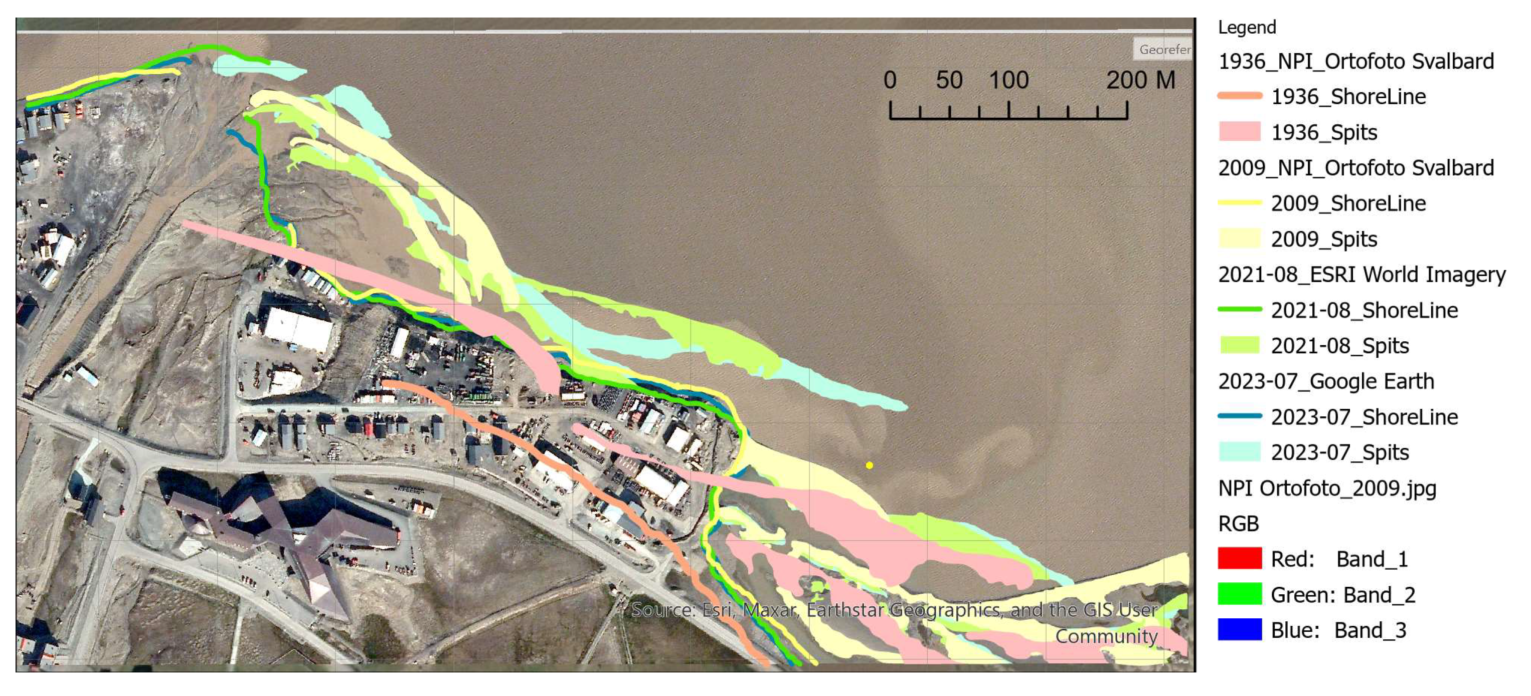
Figure A2.
All gravel spit polygon combined and presented as contours without filling. On the background of Ortophoto 2009 [26].
Figure A2.
All gravel spit polygon combined and presented as contours without filling. On the background of Ortophoto 2009 [26].
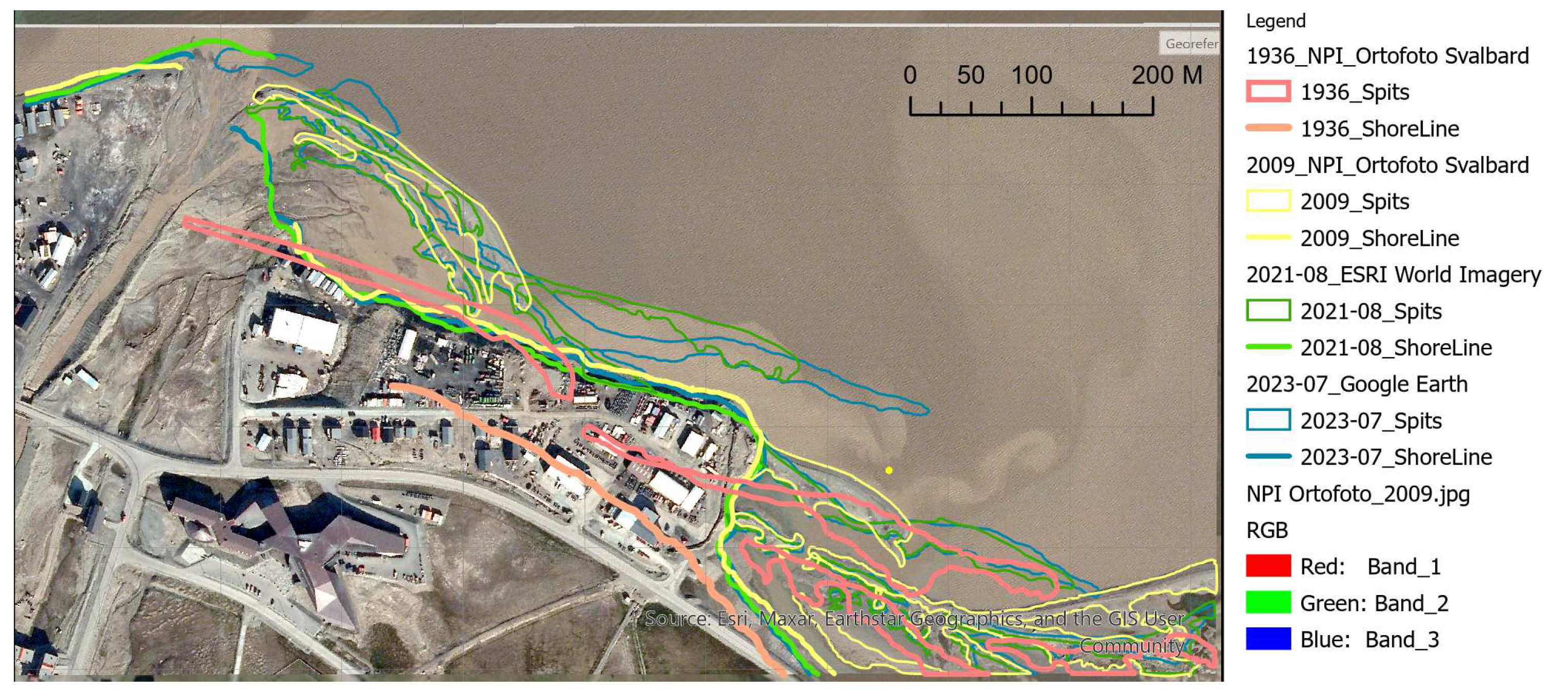
Figure A3.
Lagoon gravel spit polygons digitalised on the base and background of Ortophoto 1936 [43].
Figure A3.
Lagoon gravel spit polygons digitalised on the base and background of Ortophoto 1936 [43].
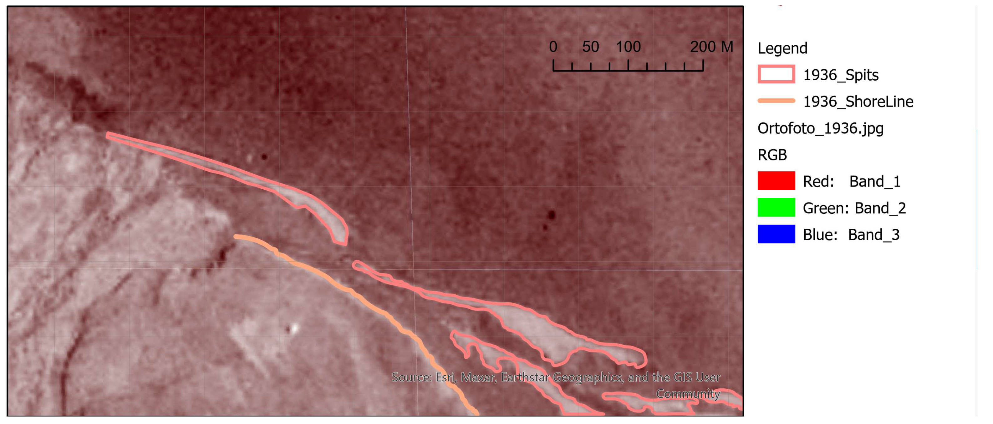
Figure A4.
Lagoon gravel spit polygons digitalised on the base and background of Ortophoto 2009 [26]
Figure A4.
Lagoon gravel spit polygons digitalised on the base and background of Ortophoto 2009 [26]
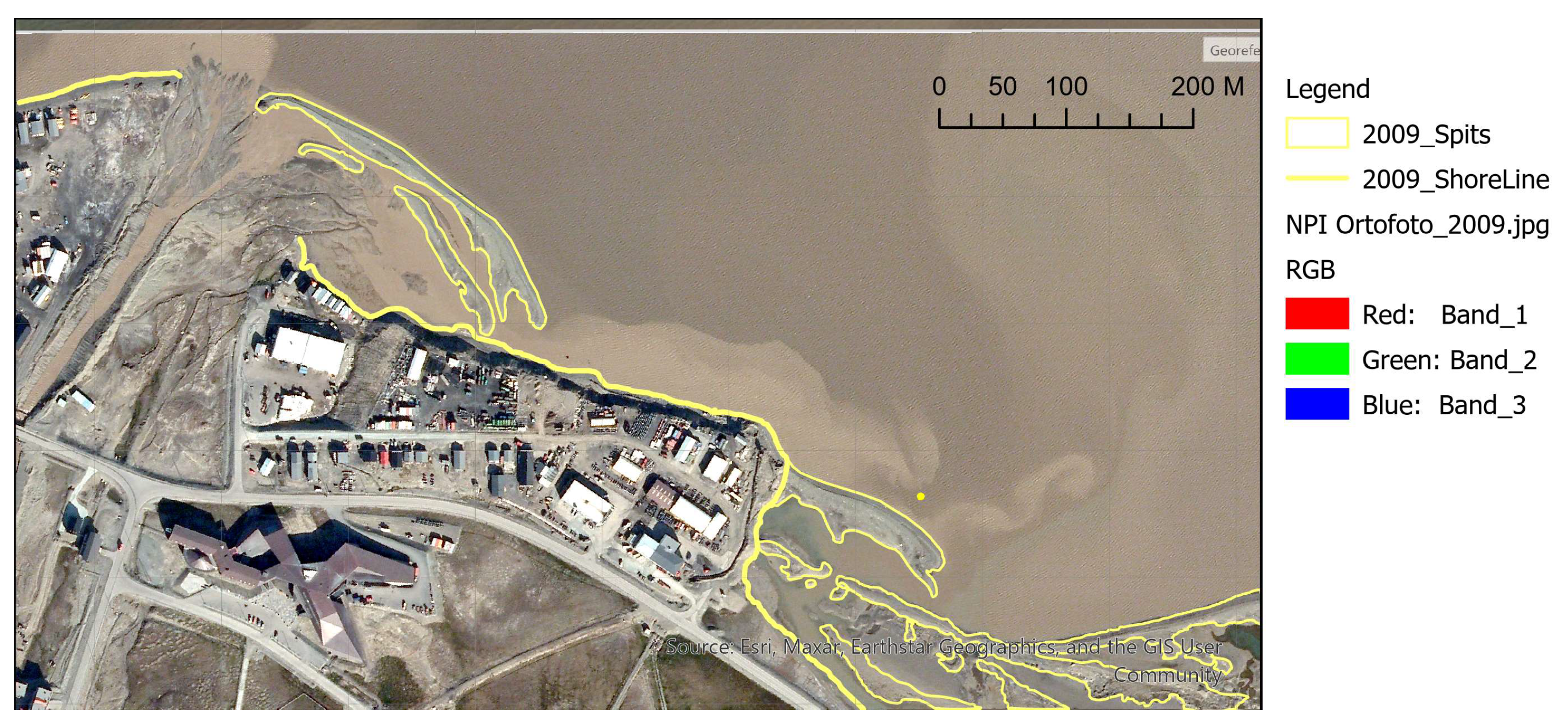
Figure A5.
Lagoon gravel spit polygons in 2021 digitalised on the base and background of ESRI basemap [44].
Figure A5.
Lagoon gravel spit polygons in 2021 digitalised on the base and background of ESRI basemap [44].
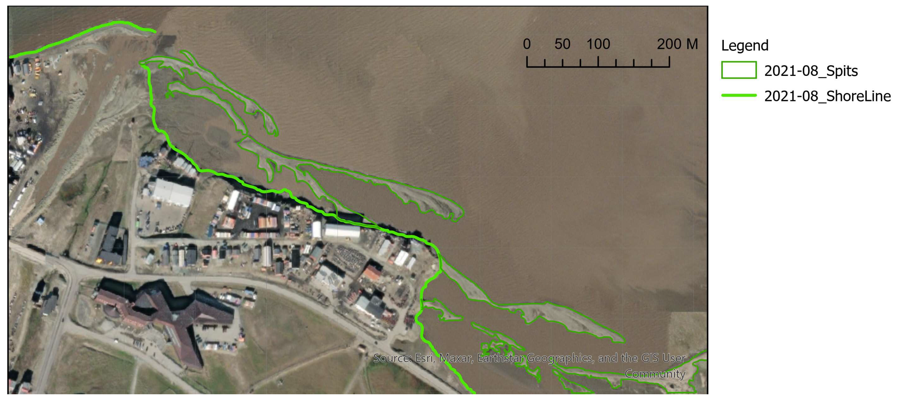
Figure A6.
Lagoon gravel spit polygons in July 2023 digitalised on the base and background of Google Earth Imagery [25].
Figure A6.
Lagoon gravel spit polygons in July 2023 digitalised on the base and background of Google Earth Imagery [25].
Appendix 2. Lagoon spit point clouds 2019-2023.
Screen shot from RiScan Pro. Point clouds for consequences of Scans from the same Scan Position (coordinates DD MM SS: 78°13′25″N 15°40′4″E - Wooden terrace near so called bird observation house). Point clouds are coloured by elevation in the Project Coordinate system and colour bar is visible in the right upper conner of the screen shots. Point001 indicates the place where the pipe with SBE inside was installed in October 2022.
Date is presented in Year-Month-Day format as it is common in RiScan Sorfware and inherite to raw data.
References
- Barnes, R.S.K. , Lagoons, in Encyclopedia of Ocean Sciences, J.H. Steele, Editor. 2001, Academic Press: Oxford. p. 1427-1438.
- Miller, C.A.; Bonsell, C.; McTigue, N.D.; Kelley, A.L. The seasonal phases of an Arctic lagoon reveal the discontinuities of pH variability and CO2 flux at the air–sea interface. Biogeosciences 2021, 18, 1203–1221. [Google Scholar] [CrossRef]
- Pedrazas, M.N.; Cardenas, M.B.; Demir, C.; Watson, J.A.; Connolly, C.T.; McClelland, J.W. Absence of ice-bonded permafrost beneath an Arctic lagoon revealed by electrical geophysics. Sci. Adv. 2020, 6, eabb5083. [Google Scholar] [CrossRef]
- McMahon, K.W.; Ambrose, W.G.; Reynolds, M.J.; Johnson, B.J.; Whiting, A.; Clough, L.M. Arctic lagoon and nearshore food webs: Relative contributions of terrestrial organic matter, phytoplankton, and phytobenthos vary with consumer foraging dynamics. Estuarine, Coast. Shelf Sci. 2021, 257. [Google Scholar] [CrossRef]
- Jenrich, M.; Angelopoulos, M.; Grosse, G.; Overduin, P.P.; Schirrmeister, L.; Nitze, I.; Biskaborn, B.K.; Liebner, S.; Grigoriev, M.; Murray, A.; et al. Thermokarst Lagoons: A Core-Based Assessment of Depositional Characteristics and an Estimate of Carbon Pools on the Bykovsky Peninsula. Front. Earth Sci. 2021, 9. [Google Scholar] [CrossRef]
- PSMSL. Valkarvai. Permanent Service for Mean Sea Level 2022; Available from: https://www.psmsl.org/data/obtaining/stations/792.php.
- Marchenko, A. , et al., Influence of vibrations on indentation and compression strength of sea ice, in IAHR International Symposium on ice. 2020, NTNU: Trondheim, Norway.
- Marchenko, A.V.; Morozov, E.G. Asymmetric tide in Lake Vallunden (Spitsbergen). Nonlinear Process. Geophys. 2013, 20, 935–944. [Google Scholar] [CrossRef]
- Morozov, E.; Marchenko, A.; Filchuk, K.; Kowalik, Z.; Marchenko, N.; Ryzhov, I. Sea ice evolution and internal wave generation due to a tidal jet in a frozen sea. Appl. Ocean Res. 2019, 87, 179–191. [Google Scholar] [CrossRef]
- Nielsen, D.M.; Pieper, P.; Barkhordarian, A.; Overduin, P.; Ilyina, T.; Brovkin, V.; Baehr, J.; Dobrynin, M. Increase in Arctic coastal erosion and its sensitivity to warming in the twenty-first century. Nat. Clim. Chang. 2022, 12, 263–270. [Google Scholar] [CrossRef]
- Ogorodov, S.; Aleksyutina, D.; Baranskaya, A.; Shabanova, N.; Shilova, O. Coastal Erosion of the Russian Arctic: An Overview. J. Coast. Res. 2020, 95, 599–604. [Google Scholar] [CrossRef]
- Tanguy, R. , et al., Pan-Arctic Assessment of Coastal Settlements and Infrastructure Vulnerable to Coastal Erosion, Sea-Level Rise, and Permafrost Thaw. Earth's Future, 2024. 12(12): p. e2024EF005013.
- Kim, D.; Jo, J.; Nam, S.-I.; Choi, K. Morphodynamic evolution of paraglacial spit complexes on a tide-influenced Arctic fjord delta (Dicksonfjorden, Svalbard). Mar. Geol. 2022, 447. [Google Scholar] [CrossRef]
- Strzelecki, M.C.; Long, A.J.; Lloyd, J.M. Post-Little Ice Age Development of a High Arctic Paraglacial Beach Complex. Permafr. Periglac. Process. 2015, 28, 4–17. [Google Scholar] [CrossRef]
- Strzelecki, M.C.; Long, A.J.; Lloyd, J.M.; Małecki, J.; Zagórski, P.; Pawłowski, Ł.; Jaskólski, M.W. The role of rapid glacier retreat and landscape transformation in controlling the post-Little Ice Age evolution of paraglacial coasts in central Spitsbergen (Billefjorden, Svalbard). Land Degrad. Dev. 2018, 29, 1962–1978. [Google Scholar] [CrossRef]
- Jaskólski, M.W.; Pawłowski, Ł.; Strzelecki, M.C. High Arctic coasts at risk—the case study of coastal zone development and degradation associated with climate changes and multidirectional human impacts in Longyearbyen (Adventfjorden, Svalbard). Land Degrad. Dev. 2018, 29, 2514–2524. [Google Scholar] [CrossRef]
- Bourriquen, M. , et al., Coastal evolution and sedimentary mobility of Brøgger Peninsula, northwest Spitsbergen. Polar Biology, 2016. 39(10): p. 1689-1698.
- Lønne, I.; Nemec, W. High-arctic fan delta recording deglaciation and environment disequilibrium. Sedimentology 2004, 51, 553–589. [Google Scholar] [CrossRef]
- Zagórski, P. Shoreline dynamics of Calypsostranda (NW Wedel Jarlsberg Land, Svalbard) during the last century. Pol. Polar Res. 2011, 32, 67–99. [Google Scholar] [CrossRef]
- Haug, F.D. and P.I. Myhre, Naturtyper på Svalbard: laguner og pollers betydning, med katalog over lokaliteter, in Kortrapport. 2016, Norsk Polarinstitutt. p. 174.
- Weslawski, J. , et al., Adventfjorden: Arctic sea in the backyard. 2011.
- Instanes, A. Incorporating climate warming scenarios in coastal permafrost engineering design – Case studies from Svalbard and northwest Russia. Cold Reg. Sci. Technol. 2016, 131, 76–87. [Google Scholar] [CrossRef]
- NCCS, Climate in Svalbard 2100 – a knowledge base for climate adaptation, E.J.F. I.Hanssen-Bauer, H.Hisdal, S.Mayer, A.B.Sandø, A.Sorteberg, Editor. 2019, The Norwegian Centre for Climate Services: Oslo. p. 105.
- ITV News. Svalbard: The remote Arctic island warming seven times faster than the global average. 2023 01.03.2023; Available from: https://www.youtube.com/watch?v=KXTPduyDamE.
- Google. Google Earth Pro Image. 2023 14.02. 2024.
- Norwegian Polar Institute. TopoSvalbard. 2024 19.03.2024]; Available from: http://toposvalbard.npolar.no/.
- Piepjohn, K. , et al. , The Geology of Longyearbyen. 2012, 2022, Longyearbyen: LoFF. [Google Scholar]
- Nordli, Ø.; Wyszyński, P.; Gjelten, H.M.; Isaksen, K.; Łupikasza, E.; Niedźwiedź, T.; Przybylak, R. Revisiting the extended Svalbard Airport monthly temperature series, and the compiled corresponding daily series 1898–2018. Polar Res. 2020, 39. [Google Scholar] [CrossRef]
- Esau, I.; Miles, V. A local climate perspective on possible development pathways for Longyearbyen, Svalbard. Polar Rec. 2024, 60. [Google Scholar] [CrossRef]
- Lapointe, F.; Karmalkar, A.V.; Bradley, R.S.; Retelle, M.J.; Wang, F. Climate extremes in Svalbard over the last two millennia are linked to atmospheric blocking. Nat. Commun. 2024, 15, 1–10. [Google Scholar] [CrossRef]
- Bogen, J. and T.E. Bønsnes, Erosion and sediment transport in High Arctic rivers, Svalbard. Polar Research, 2003. 22(2): p. 175-189.
- Pallesen, L.M. , Sediment source-to-sink in a warming Arctic; thawing moraines, slope processes and river erosion in Longyeardalen, Svalbard, in Institutt for geovitenskap og petroleum. 2022, NTNU: Trondheim. p. 114.
- Winther, S.N.; Gudmestad, O.T. Impact of and solutions to effects of climate changes for Longyearbyen, Svalbard, Norway. IOP Conf. Series: Mater. Sci. Eng. 2023, 1294, 012036. [Google Scholar] [CrossRef]
- Nygård Jakobsen, A. , Omfattende planer for å sikre Longyearbyen mot naturkatastrofer (Comprehensive plans to secure Longyearbyen against natural disasters), in NRK web. 2017, NRK: www.nrk.no.
- Ottem, M.J.D. , The Longyearelva River-to-Ocean System; Monitoring an anthropogenic arctic fluvial system in changing climate over short and long timescales, in Institutt for geovitenskap og petroleum. 2022, NTNU: Trondheim. p. 119.
- Longyearbyen Lokalstyre. Flomsikringstiltak Longyearelva (Flood protection measures at Longyear river). 2016 13.11.2016; Available from: https://www.lokalstyre.no/flomsikringstiltak-longyearelva.5920630-209814.html.
- Kowalik, Z.; Marchenko, A.; Brazhnikov, D.; Marchenko, N. Tidal currents in the western Svalbard Fjords. Oceanologia 2015, 57, 318–327. [Google Scholar] [CrossRef]
- Marchenko, A. and Z. Kowalik, Investigation of Ocean Currents in Navigational Straits of Spitsbergen, in Marine Navigation. Marine Navigation and Safety of Sea Transportation. 2017, CRC Press. p. 426.
- Tide Times and Tide Charts for the World. Tide Times for Longyearbyen, Spitsbergen. 2024; Available from: https://www.tide-forecast.com/locations/Longyearbyen-Spitsbergen/tides/latest.
- Marchenko, N. , et al., Monitoring of sea currents and waves in Spitsbergen fjords, in Geophysical Research Abstracts. 2014.
- Marchenko, N. and A. Marchenko, Ice formation, Growth and Dynamics in Arctic Lagoon (Spitsbergen), in IAHR International Symposium on ice. 2022: Montreal, Canada.
- Marchenko, N. , Coastal Ice Rubbles in Isfjorden (Spitsbergen), in Proceedings of the 27th International Conference on Port and Ocean Engineering under Arctic Conditions (POAC-23).. 2023: Glasgow, United Kingdom. p. 11.
- Norwegian Polar Institute. Ortofoto Svalbard 1936. Svalbardkartet 2024 14.02.2024]; Available from: https://geokart.npolar.no/Html5Viewer/index.html?viewer=Svalbardkartet.
- ESRI and MAXAR. World Imagery. 2023; Available from: https://www.arcgis.com/apps/mapviewer/index.html?webmap=c03a526d94704bfb839445e80de95495.
- Riegl. Terrestrial Laser Scanning. 2024; Available from: http://www.riegl.com/nc/products/terrestrial-scanning/.
- Riegl. RiSCAN PRO. Operating and Processing Software for RIEGL 3D Laser Scanners. 2021; Available from: http://www.riegl.com/uploads/tx_pxpriegldownloads/11_DataSheet_RiSCAN-PRO_2016-09-19.pdf.
- Sea-Bird Scientific. SBE 39plus Temperature (Depth) Recorder. 2025; Available from: https://www.seabird.com/moored/sbe-39plus-temperature-depth-recorder/family?productCategoryId=54627473774.
- Geoengineer. Step-by-Step Guide for Grain Size Analysis. 2024; Available from: https://www.geoengineer.org/education/laboratory-testing/step-by-step-guide-for-grain-size-analysis.
- Wentworth, C.K. A Scale of Grade and Class Terms for Clastic Sediments. J. Geol. 1922, 30, 377–392. [Google Scholar] [CrossRef]
- Magilligan, F.J.; Roberts, M.O.; Marti, M.; Renshaw, C.E. The impact of run-of-river dams on sediment longitudinal connectivity and downstream channel equilibrium. Geomorphology 2020, 376, 107568. [Google Scholar] [CrossRef]
- van Rijn, L.C. , Principles of sediment transport in rivers, estuaries and coastal seas. . 1993, 2017, The Netherlands: Aquapublications. [Google Scholar]
- O’grady, J.; Babanin, A.; McInnes, K. Downscaling Future Longshore Sediment Transport in South Eastern Australia. J. Mar. Sci. Eng. 2019, 7, 289. [Google Scholar] [CrossRef]
- Li, L.; Barry, D. Wave-induced beach groundwater flow. Adv. Water Resour. 2000, 23, 325–337. [Google Scholar] [CrossRef]
- Marchenko, A., V. , et al., Monitoring of thermodynamic state of soil near Arctic pipeline landfall. Vesti gazovoy nauki, 2013. 3 (14): p. 202-211.
- Fomin, Y.V.; Zhmur, V.V.; Marchenko, A.V. Transient seawater inflow into seacoast aquifers. Water Resour. 2017, 44, 61–68. [Google Scholar] [CrossRef]
- Zhmur, V.V.; Fomin, Y.V.; Marchenko, A.V. Groundwater Table Formation in the Coastal Zone over a Bed with Arbitrary Shape. Water Resour. 2018, 45, 553–559. [Google Scholar] [CrossRef]
- Li, L.; Barry, D.; Pattiaratchi, C.; Masselink, G. BeachWin: modelling groundwater effects on swash sediment transport and beach profile changes. Environ. Model. Softw. 2002, 17, 313–320. [Google Scholar] [CrossRef]
- Horn, D.P. Beach groundwater dynamics. Geomorphology 2002, 48, 121–146. [Google Scholar] [CrossRef]
Figure 1.
Longyearbyen lagoon location. a) On the Google Earth [25] b) On the map of Spitsbergen from Toposvalbard [26].
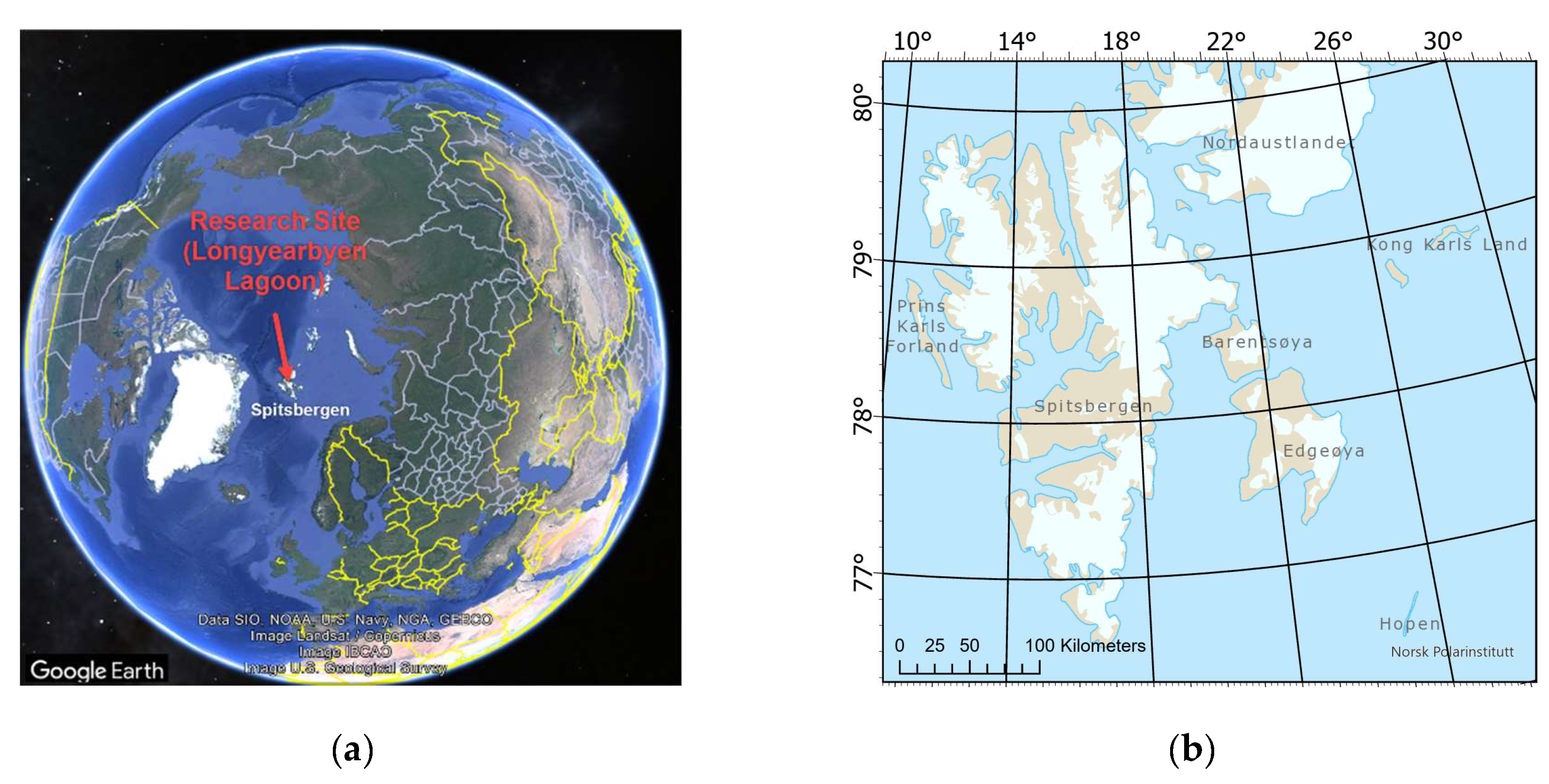
Figure 2.
Longyearbyen lagoon observation site (yellow rectangle). On the base of the map, fixing the state of 2009 [26]. Green lines show shoreline and spit contour as for July 2023, reconstructed by Google map Imagery [25]. Points indicate the locations of gravel spit end at the beginning (February 2019) and at the end (February 2024) observation. Violet arrow line – sewer pipe.
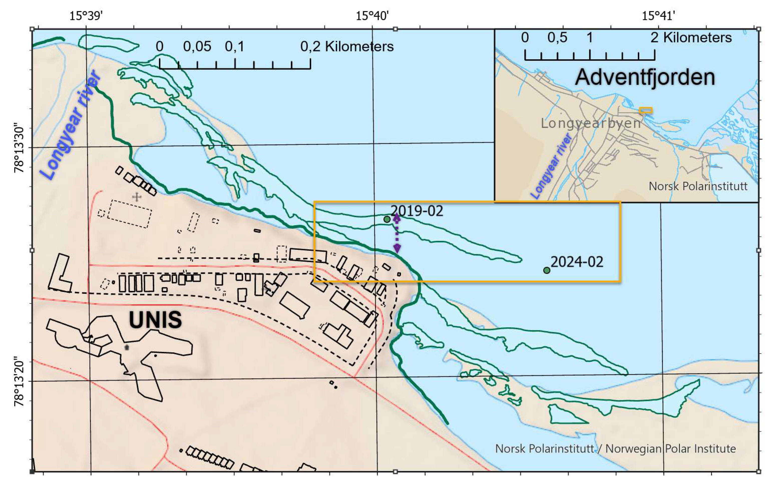
Figure 2.
Scheme of equipment deployment. Made on the background of Google Earth Image, July 2023 [25]. Small circles (orange and green)– Laser scanning positions on spit with year indication. Green pentagon – Repeated scan position. White/green quadrats – ADV deployment. Red circle – Pipe with SBE inside. Red line – Lagoon spit in September 2022, Blue line – Lagoon spit in October 2023. Reconstructed on the base of laser scanning (see corresponding section).
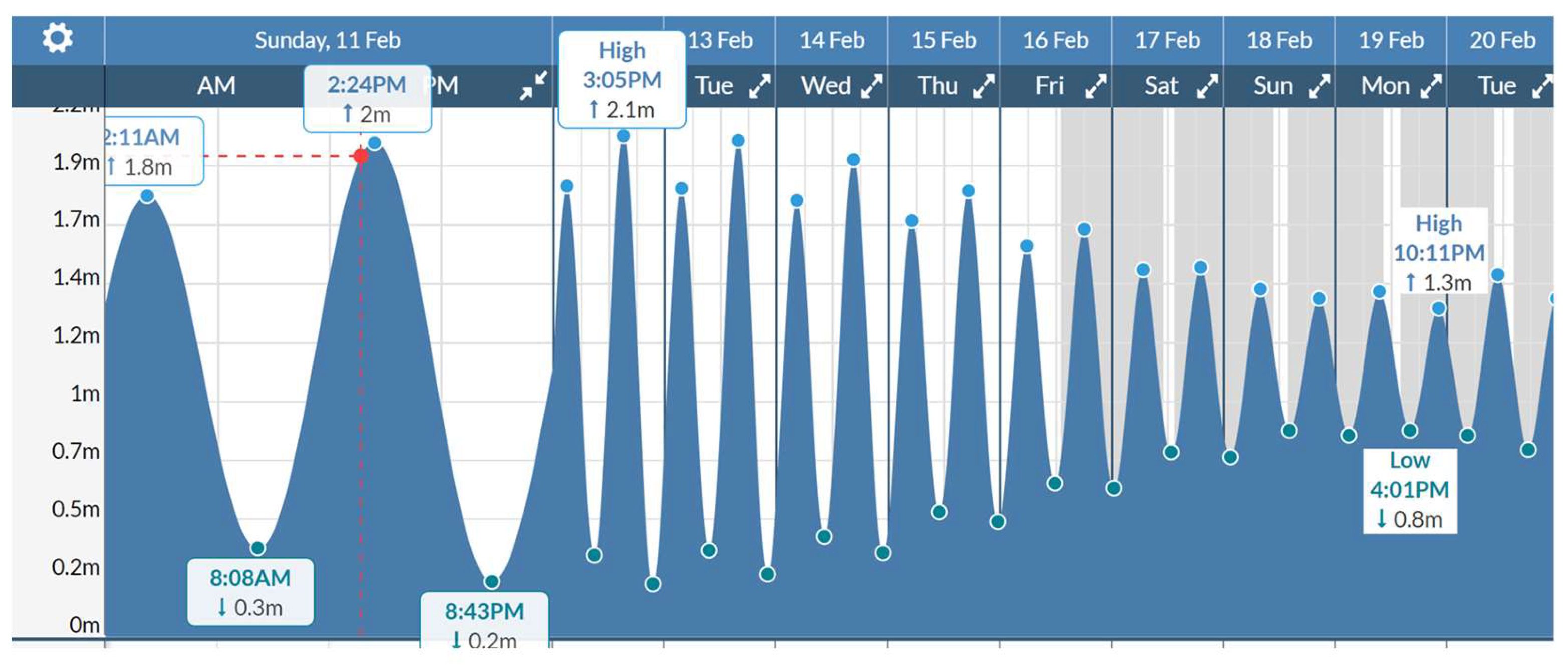
Figure 4.
Scheme of equipment deployment. Made on the background of Google Earth Image, July 2023 [25]. Small circles (orange and green)– Laser scanning positions on spit with year indication. Green pentagon – Repeated scan position. White/green quadrats – ADV deployment. Red circle – Pipe with SBE inside. Red line – Lagoon spit in September 2022, Blue line – Lagoon spit in October 2023. Reconstructed on the base of laser scanning (see corresponding section).
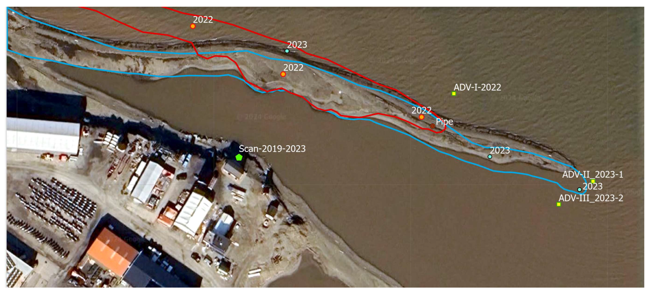
Figure 5.
Low tide scanning panorama (1 October 2023. 09:48 CET - Central European Time or Local time).
Figure 5.
Low tide scanning panorama (1 October 2023. 09:48 CET - Central European Time or Local time).
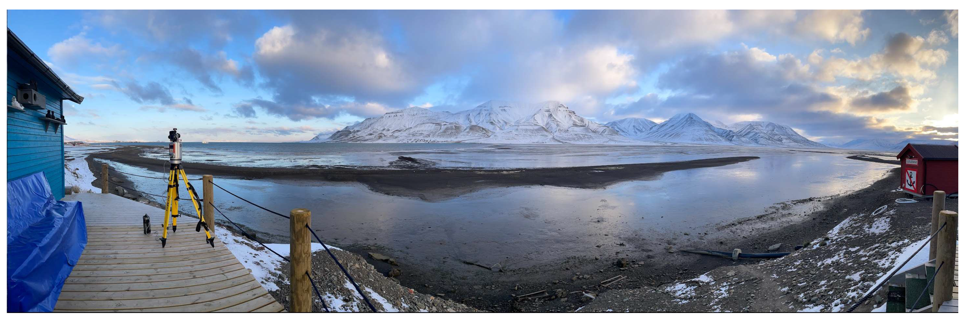
Figure 6.
Screenshot from RiScan Pro software showing the "2019-2023_ALL" project. This view integrates all critical scans, with individual scans cataloged in the object inspector on the right. They are identified by unique names that denote their respective dates and times of scanning in UTC. The main panel, set against a black background, displays two selected scans (made 30 September 2019 and 5 October 2023), visualized according to height within the project's coordinate system. The color bar (upper right corner of the main black panel) shows the altitude palette for 3D point clouds of the spits from 32.1 m to 34.1 m. Everything above 34.1 is colored pink, and everything below 32.1 is colored bright light blue. Light yellow window (left low corner) shows scan date, size of file, number of captured points and settings, defining scan accuracy and range.
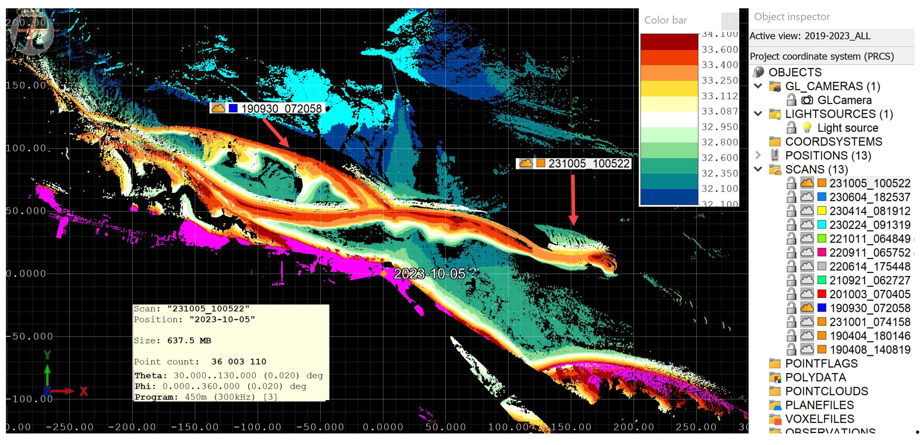
Figure 7.
Measurement of ground water level inside the pit with sensor SBE1 deployed inside test pipe. PS is the location of water pressure measurement by the sensor SBE1..
Figure 7.
Measurement of ground water level inside the pit with sensor SBE1 deployed inside test pipe. PS is the location of water pressure measurement by the sensor SBE1..
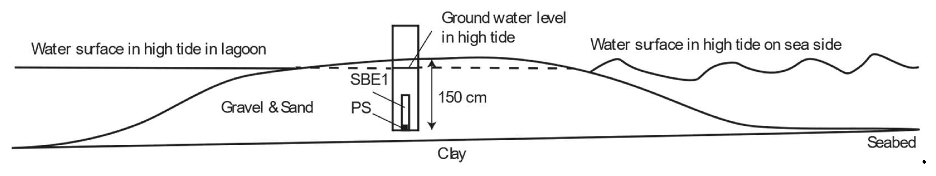
Figure 8.
Organizing of research site for observation of ground water level on the spit tip on October 10, 2022.
Figure 8.
Organizing of research site for observation of ground water level on the spit tip on October 10, 2022.
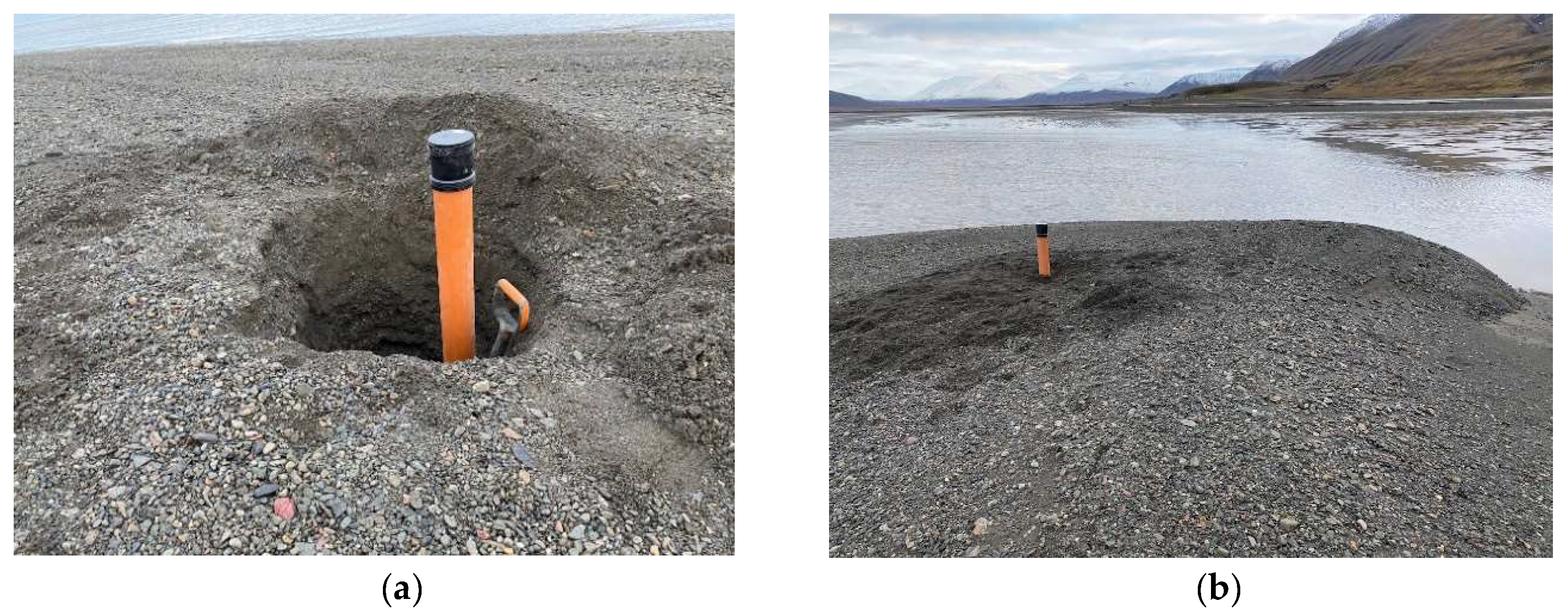
Figure 9.
Schematic (a) and photographs (b) of installation of acoustic Doppler velocimeter (ADV) at seabed with metal frame. Sensor SBE2 was mounted on the frame leg. Symbol MP marks the location of water velocity measurement. Symbols PS mark the locations of water pressure sensor.
Figure 9.
Schematic (a) and photographs (b) of installation of acoustic Doppler velocimeter (ADV) at seabed with metal frame. Sensor SBE2 was mounted on the frame leg. Symbol MP marks the location of water velocity measurement. Symbols PS mark the locations of water pressure sensor.
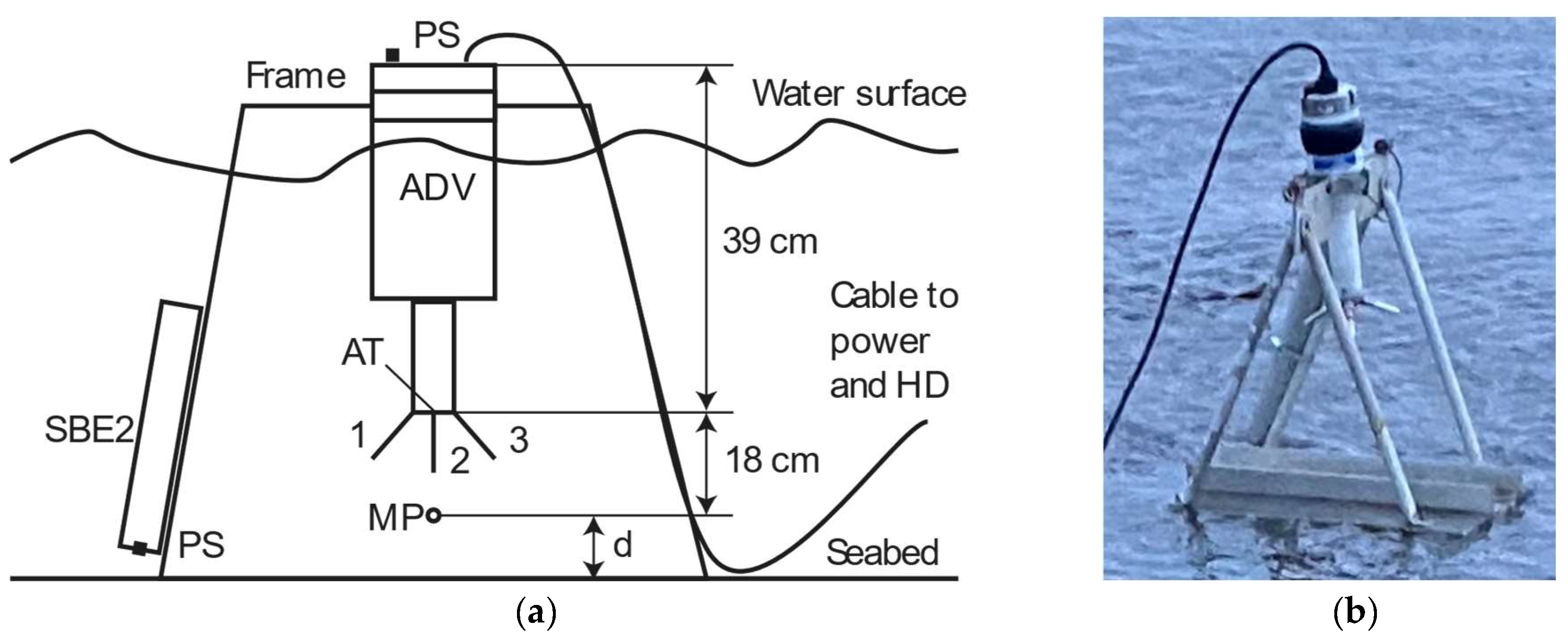
Figure 10.
Deployment of ADV on October 12, 12:23 UTC, 2022, (a) and on October 2, 8:35 UTC, 2023, (b).
Figure 10.
Deployment of ADV on October 12, 12:23 UTC, 2022, (a) and on October 2, 8:35 UTC, 2023, (b).
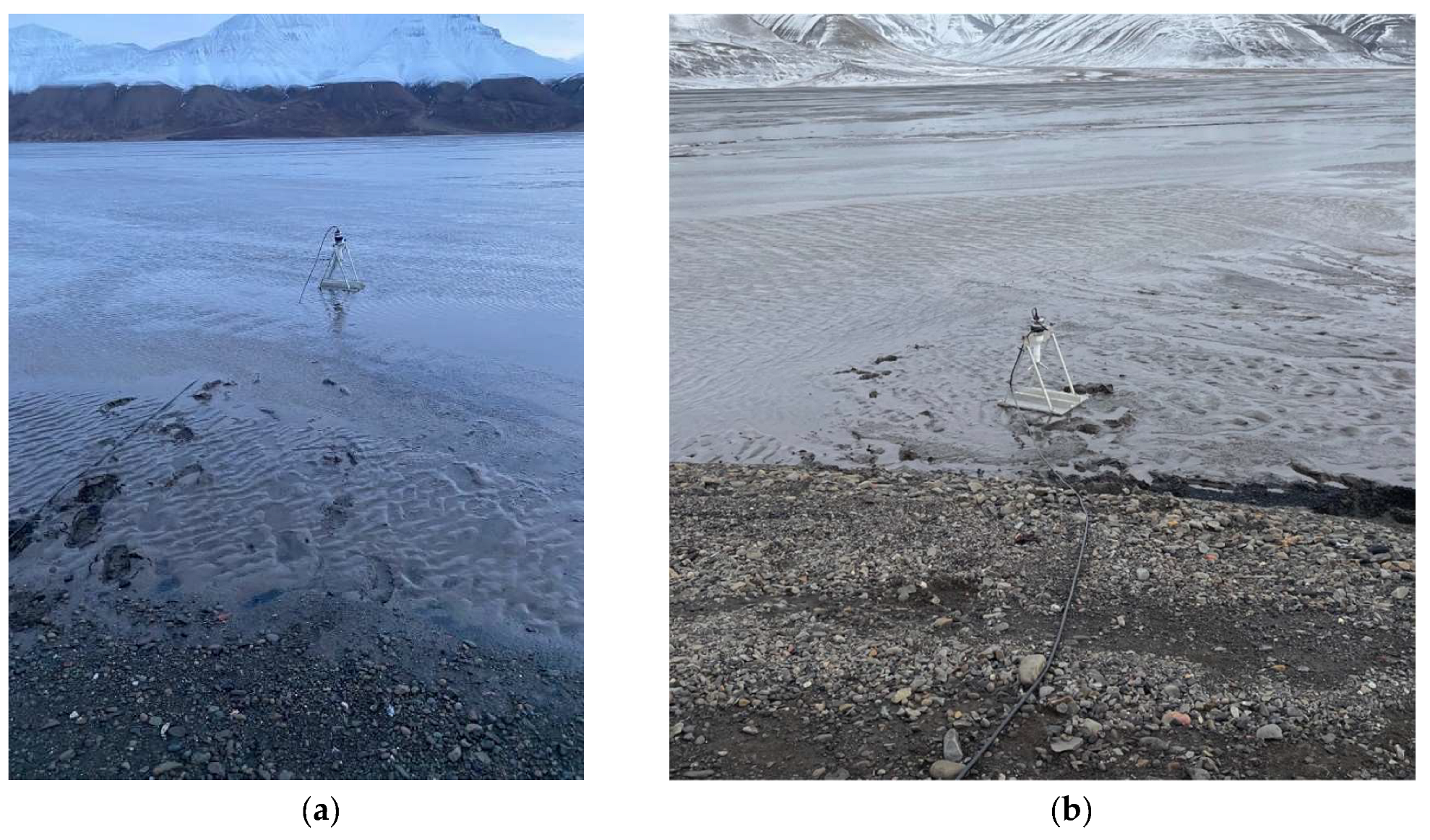
Figure 11.
Scheme of samples collection places. Made on the background of Google Earth Image showing spit location in July 2023 [25].
Figure 11.
Scheme of samples collection places. Made on the background of Google Earth Image showing spit location in July 2023 [25].
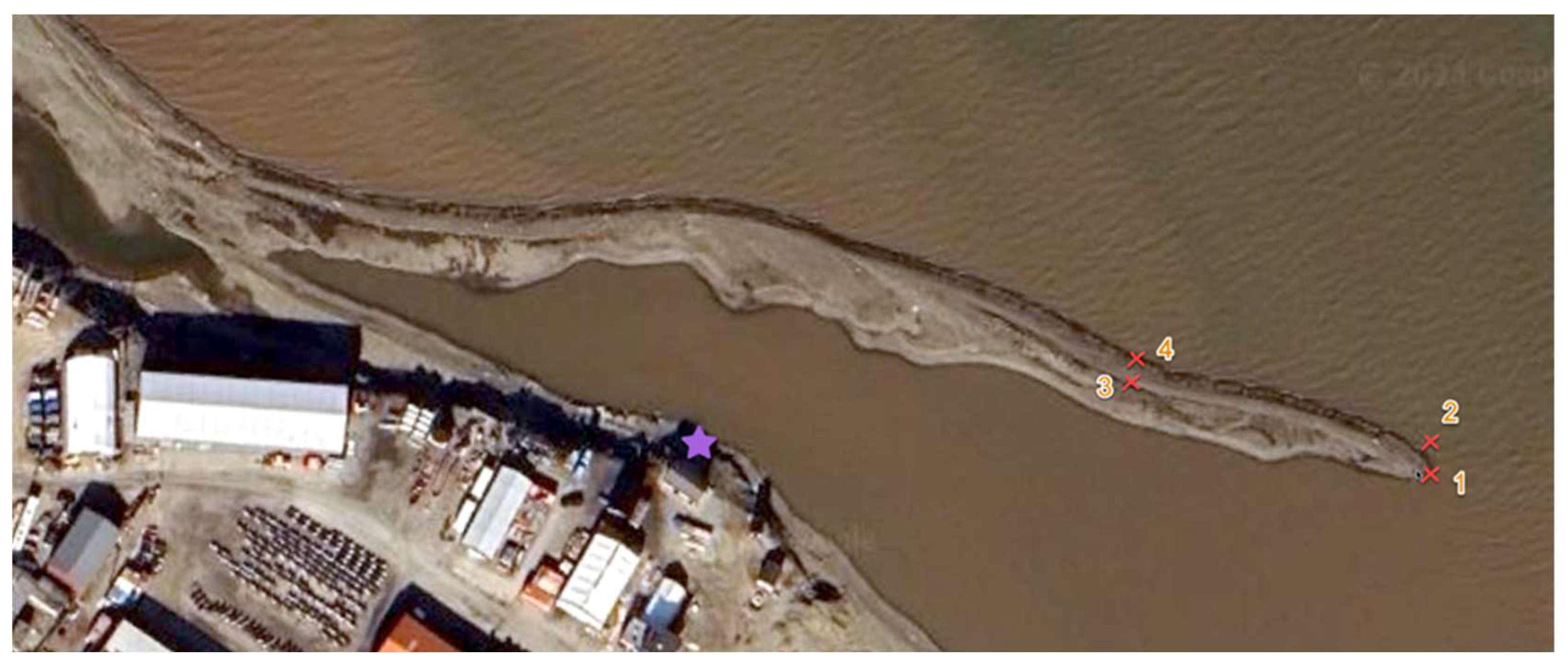
Figure 12.
Sediment samples from the advanced part of the spit (the spit tip). (a) - Sample 1. From the upper part of slope at tip of spit; (b) - Sample 2. From the shallow near the tip of spit; (c) - Sample 2 after processing.
Figure 12.
Sediment samples from the advanced part of the spit (the spit tip). (a) - Sample 1. From the upper part of slope at tip of spit; (b) - Sample 2. From the shallow near the tip of spit; (c) - Sample 2 after processing.
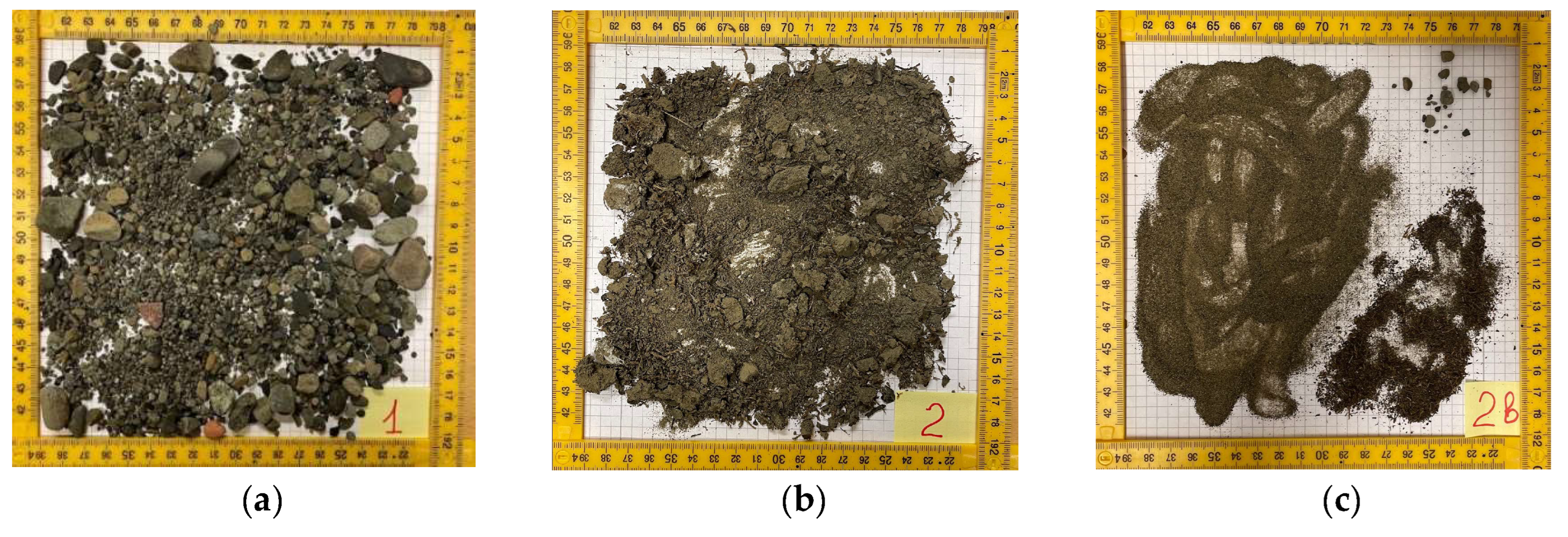
Figure 13.
Sediment samples from the middle part of the spit. (a) - Sample 3. From the ridge of the spit; (b) - Sample 4. From the spit beach.
Figure 13.
Sediment samples from the middle part of the spit. (a) - Sample 3. From the ridge of the spit; (b) - Sample 4. From the spit beach.
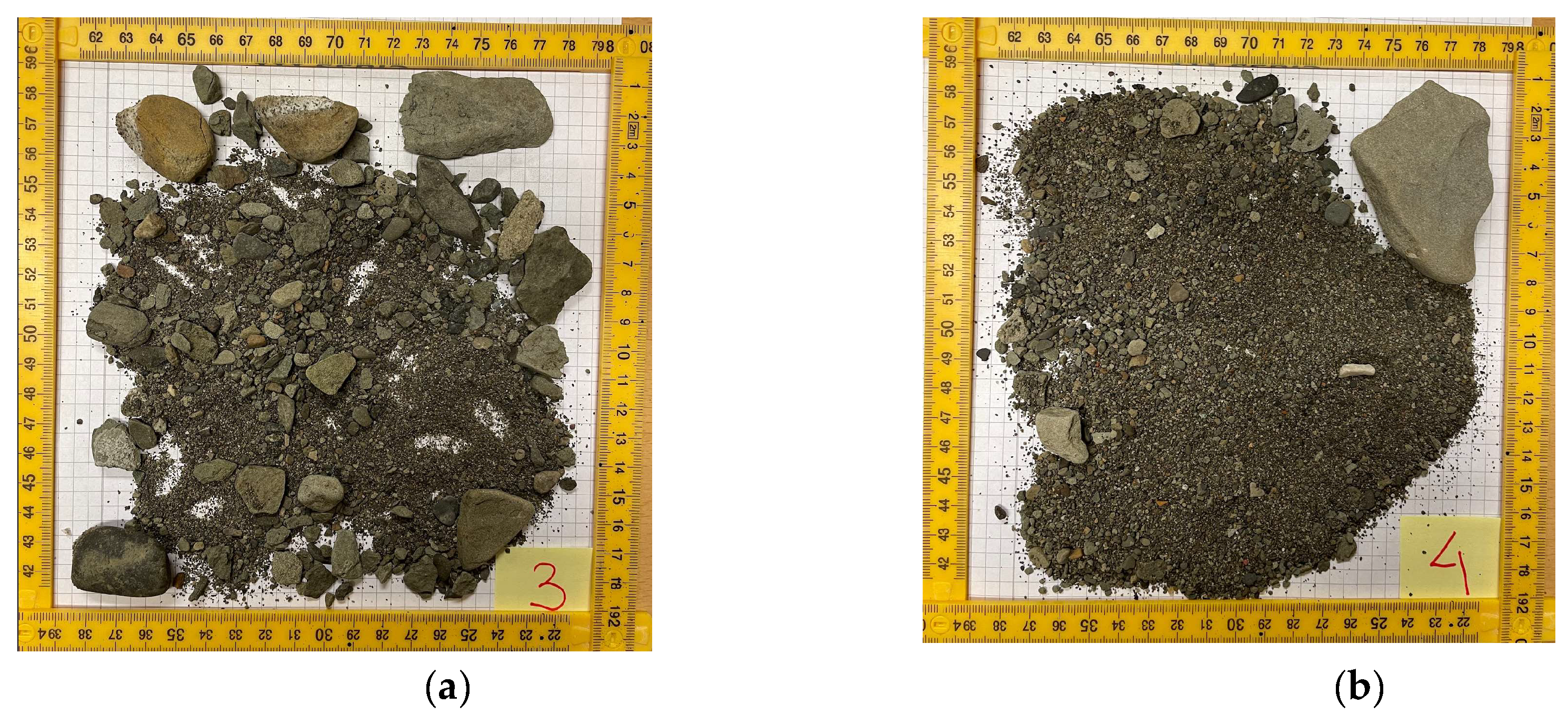
Figure 14.
Shorelines and gravel spit contours in 1934, 2009, 2021 and 2023 on the background of Ortofoto 2009 [25].
Figure 14.
Shorelines and gravel spit contours in 1934, 2009, 2021 and 2023 on the background of Ortofoto 2009 [25].
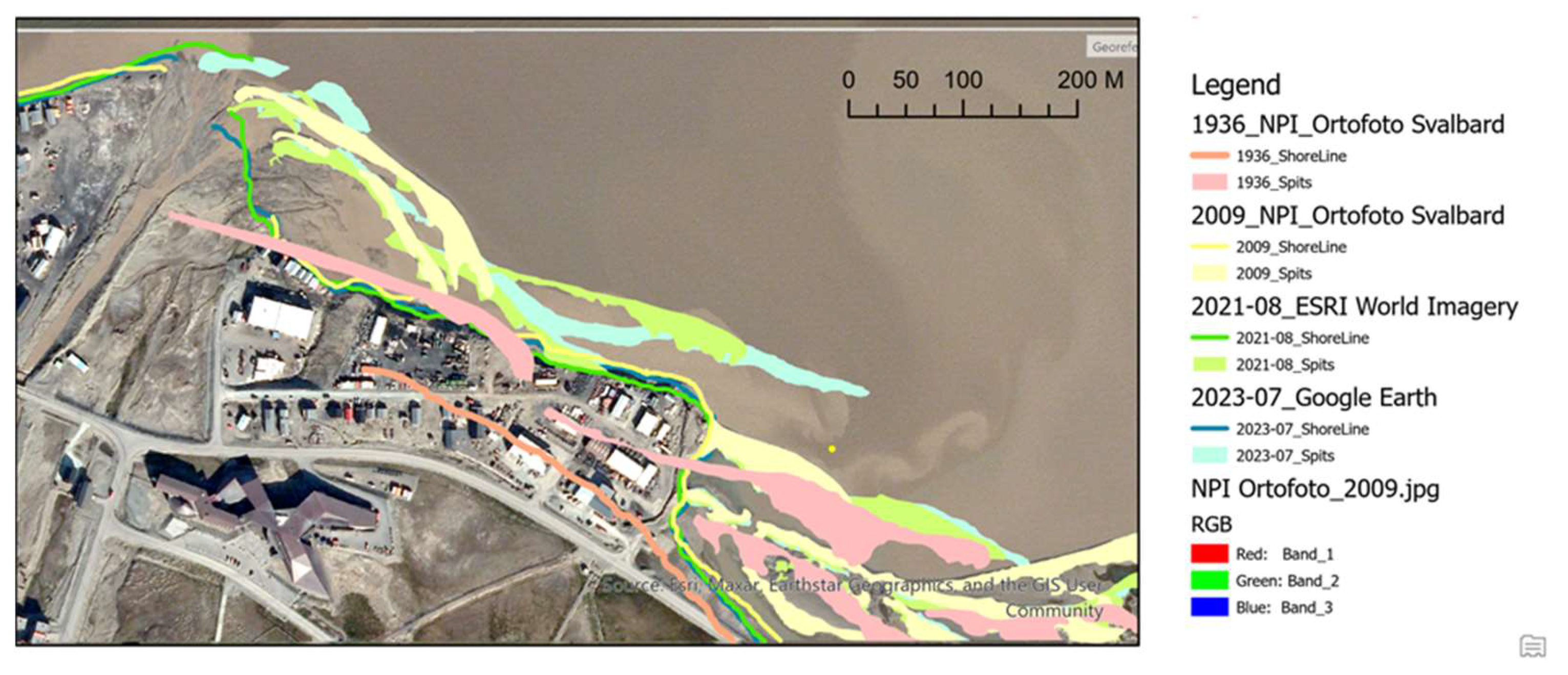
Figure 15.
Lagoon spit movement from 30 September 2019 till 05 October 2023, reflected by contours of spit presenting 10 cm point cloud slice in upper part of the spit ridge (33.5-33.6 m elevation in project coordinate system). Each point cloud is presenting in own color and arrows with the date mark the spit end at corresponding day. Red arrows indicate autumn scans and green arrows – spring scans. Axis show distance in meters.
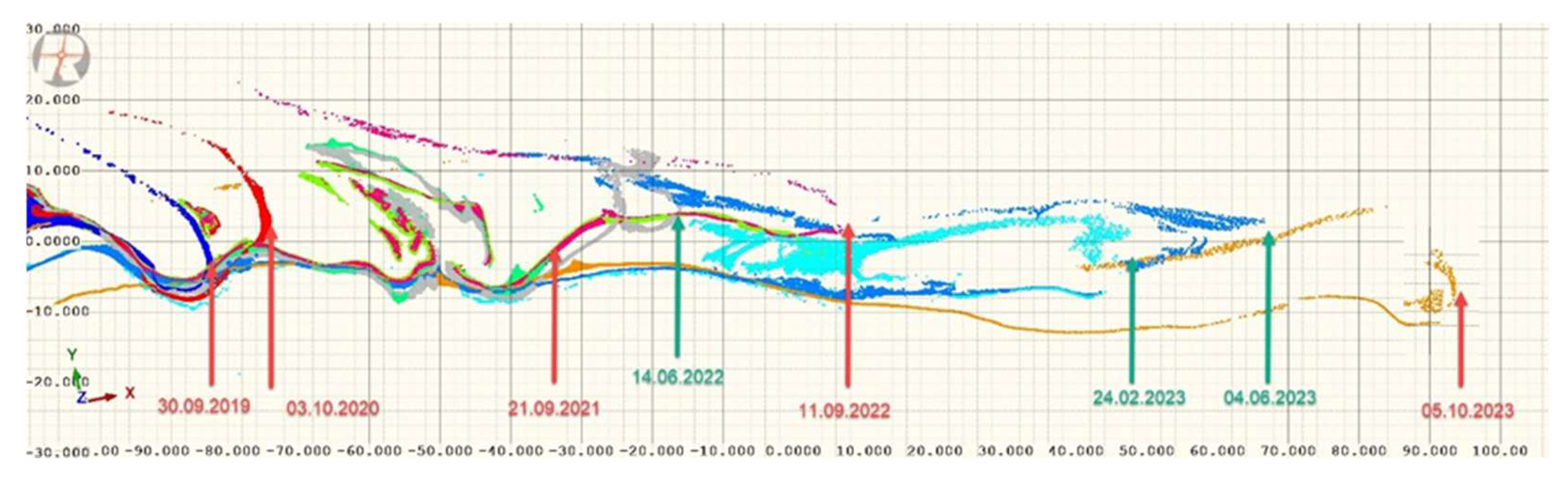
Figure 16.
Levels of sea water measured by sensors SBE3 (blue lines) and SBE2 (green line) (a). Levels of sea water and ground water measured by sensors SBE2 (green line) and SBE1 (yellow line) versus time in October 12-22, 2022.
Figure 16.
Levels of sea water measured by sensors SBE3 (blue lines) and SBE2 (green line) (a). Levels of sea water and ground water measured by sensors SBE2 (green line) and SBE1 (yellow line) versus time in October 12-22, 2022.
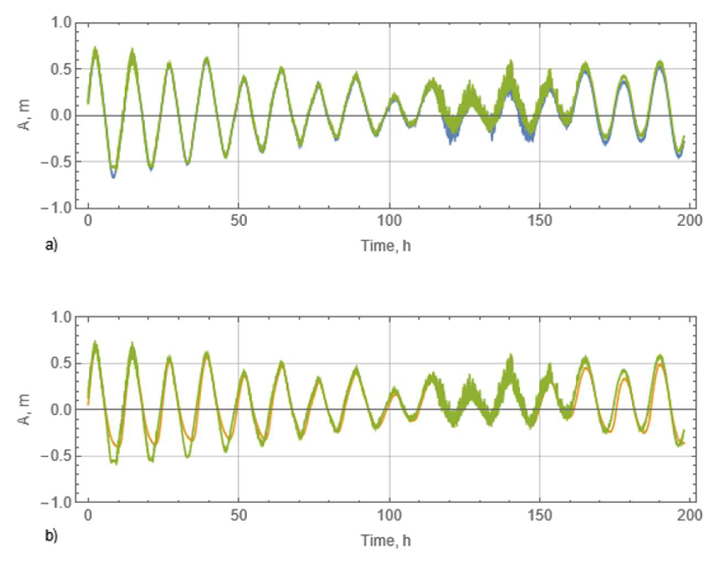
Figure 17.
Levels of sea water and ground water measured by sensors SBE3 (blue lines) and SBE1 (yellow line) versus time from October 12, 2022, to February 23, 2023 (a). Zoomed fragment of the seawater levels versus time over 100 h in the end of January 2023 (b). .
Figure 17.
Levels of sea water and ground water measured by sensors SBE3 (blue lines) and SBE1 (yellow line) versus time from October 12, 2022, to February 23, 2023 (a). Zoomed fragment of the seawater levels versus time over 100 h in the end of January 2023 (b). .
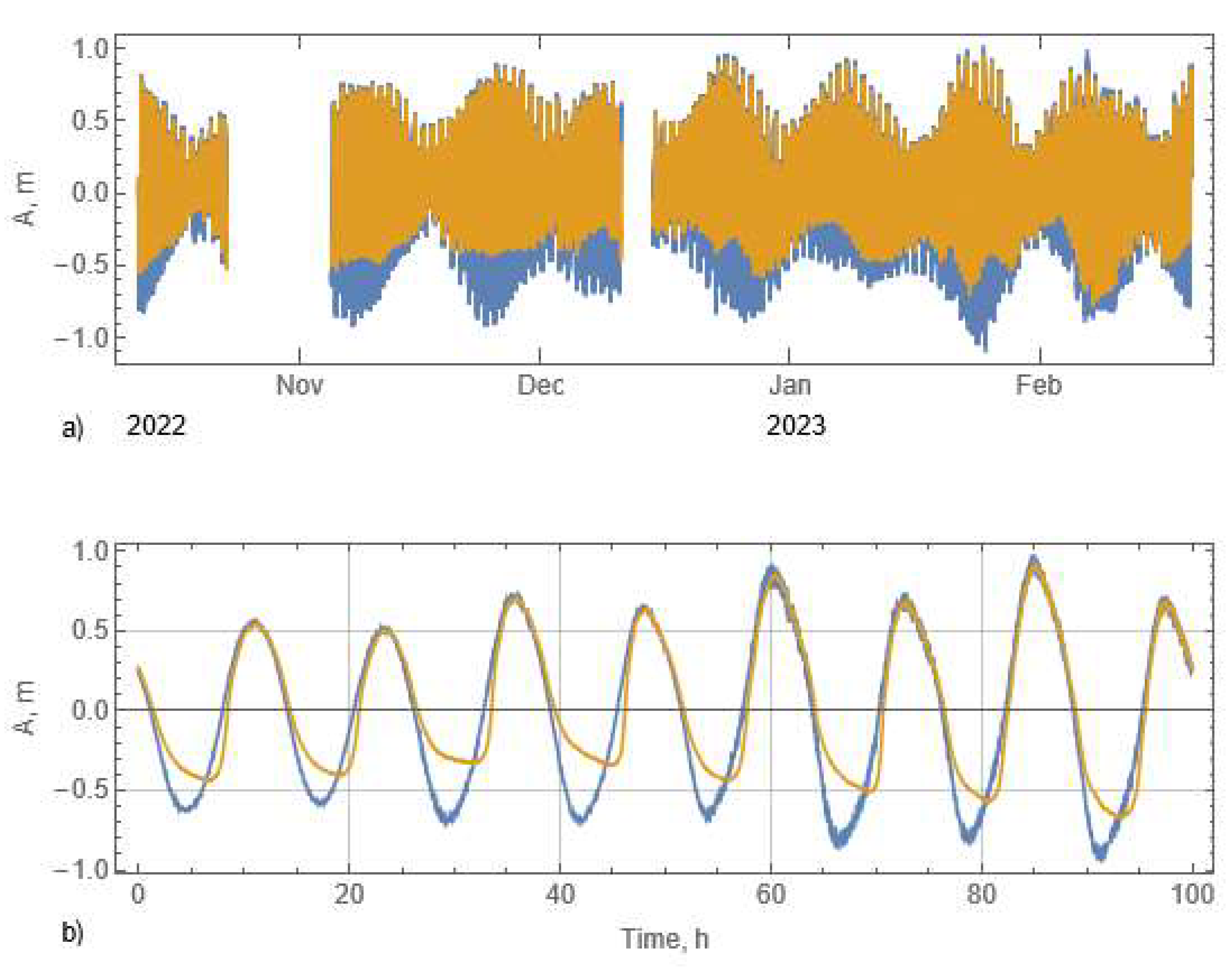
Figure 18.
Results of measurements in location ADV-I: (a) mean water speed versus time, (b) fluctuations of North and East components of water velocity measured with 10 Hz frequency (blue points) and mean water velocity (yellow points), (c) standard deviation of water speed, and (d) Reynolds stresses versus time. Time is calculated from October 12, 00:00 UTC, 2022.
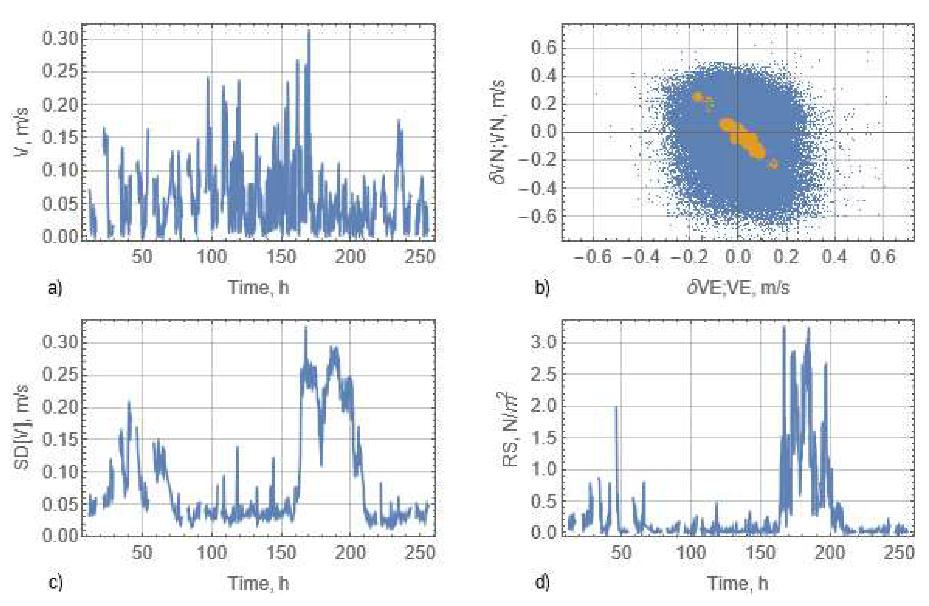
Figure 19.
Results of measurements in locations ADV-I and ADV-III: (a) Changes water levels measured in the harbour (line H) and by ADV pressure sensor in locations ADV-II and ADV-III, (b) mean water speed, (c) standard deviation of water speed, and (d) Reynolds stresses versus time. Time is calculated from October 2, 00:00 UTC, 2023. Vertical black lines separate measurements ADV-II and ADV-III. .
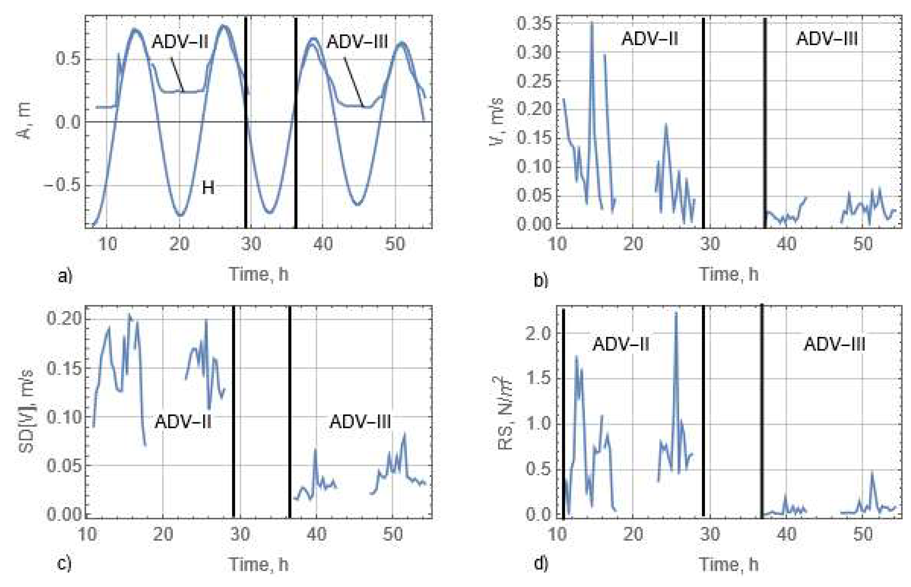
Figure 20.
East and North water velocities components measured in locations ADV-II (a) and ADV-III (b). Blue and yellow points show respectively fluctuations of water velocities measured with 10 Hz sampling frequency and mean water velocities.
Figure 20.
East and North water velocities components measured in locations ADV-II (a) and ADV-III (b). Blue and yellow points show respectively fluctuations of water velocities measured with 10 Hz sampling frequency and mean water velocities.
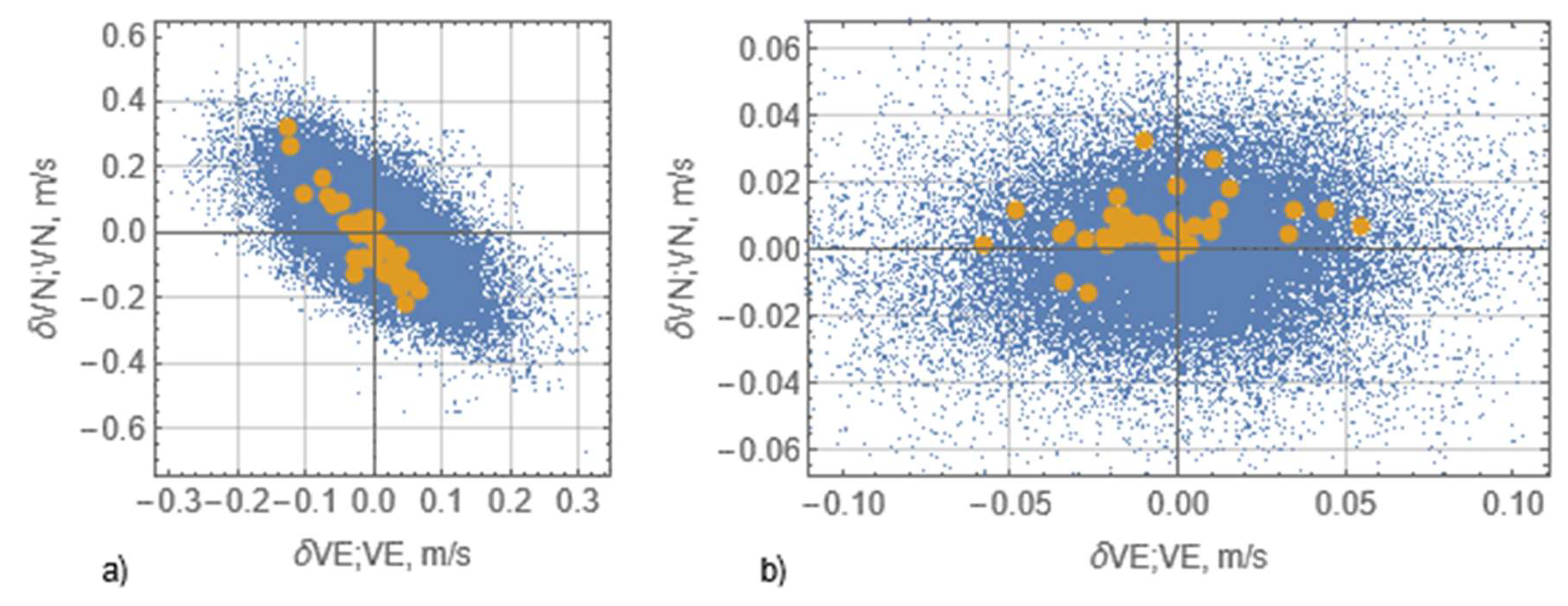
Figure 21.
Grain size distribution curves. (a) Four positions on gravel spit (see Figure 11, Figure 12 and Figure 13) in different colours; (b)Solid line - shore sediments of mixed top 2m layer sample; Dashed line shows the granulometric composition of the sediments with removed grains with a diameter of less than 1 mm.
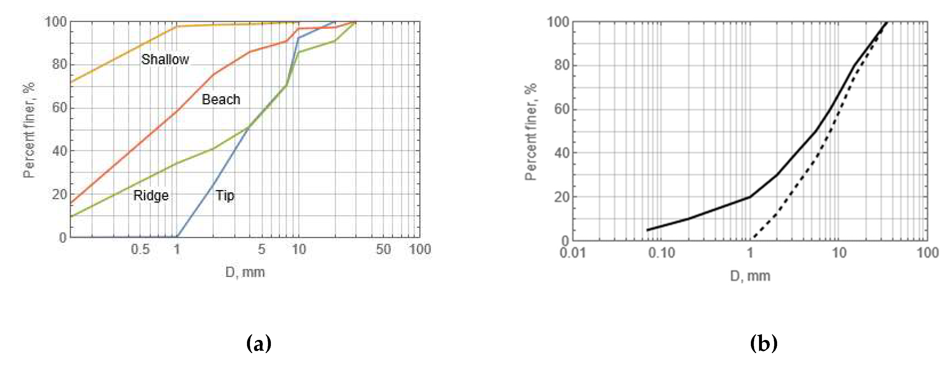
Figure 22.
Lines S corresponding
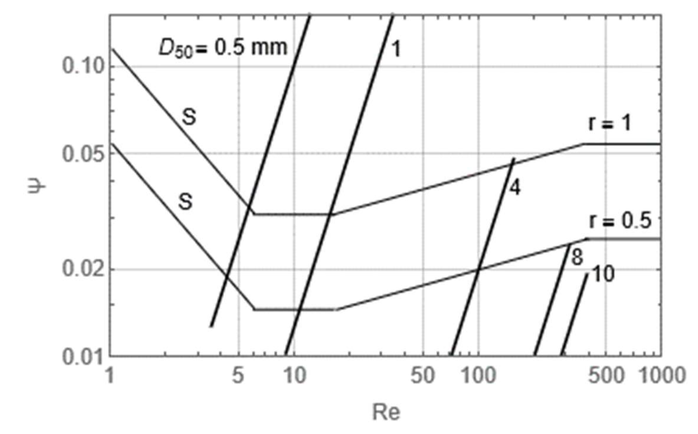
Figure 23.
ADV buried by gravel on October 3, 2023, 7:46 UTC. Horizontal dimension of the frame is 45 cm. Vertical dimension of white housing of ADV above gravel is 20 cm.
Figure 23.
ADV buried by gravel on October 3, 2023, 7:46 UTC. Horizontal dimension of the frame is 45 cm. Vertical dimension of white housing of ADV above gravel is 20 cm.
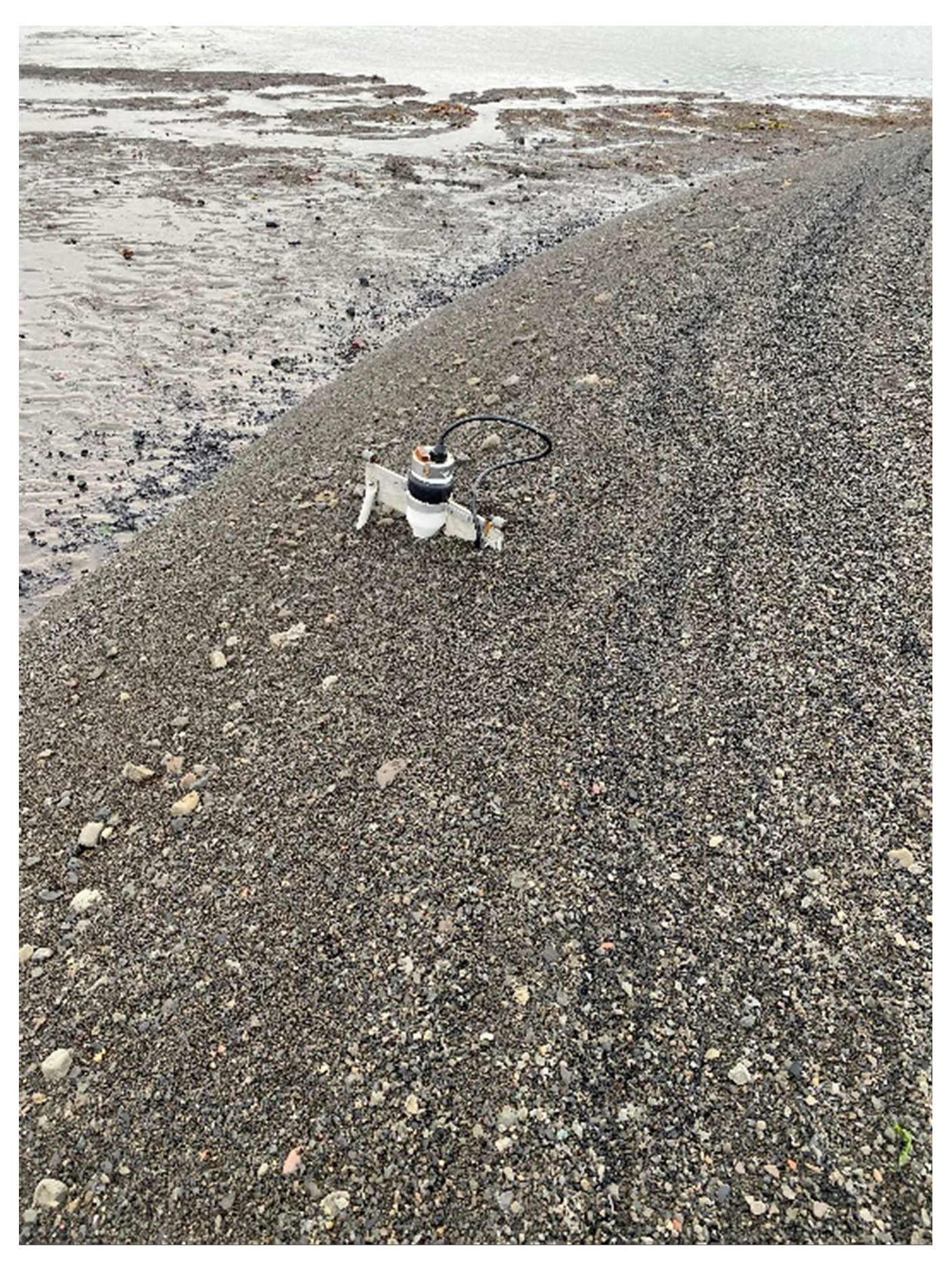
Figure 24.
Over wash of the spit on October 2 (a) and October 5 (b), 2023. The location of ADV battery on the spit tip is visible in Figure a.
Figure 24.
Over wash of the spit on October 2 (a) and October 5 (b), 2023. The location of ADV battery on the spit tip is visible in Figure a.
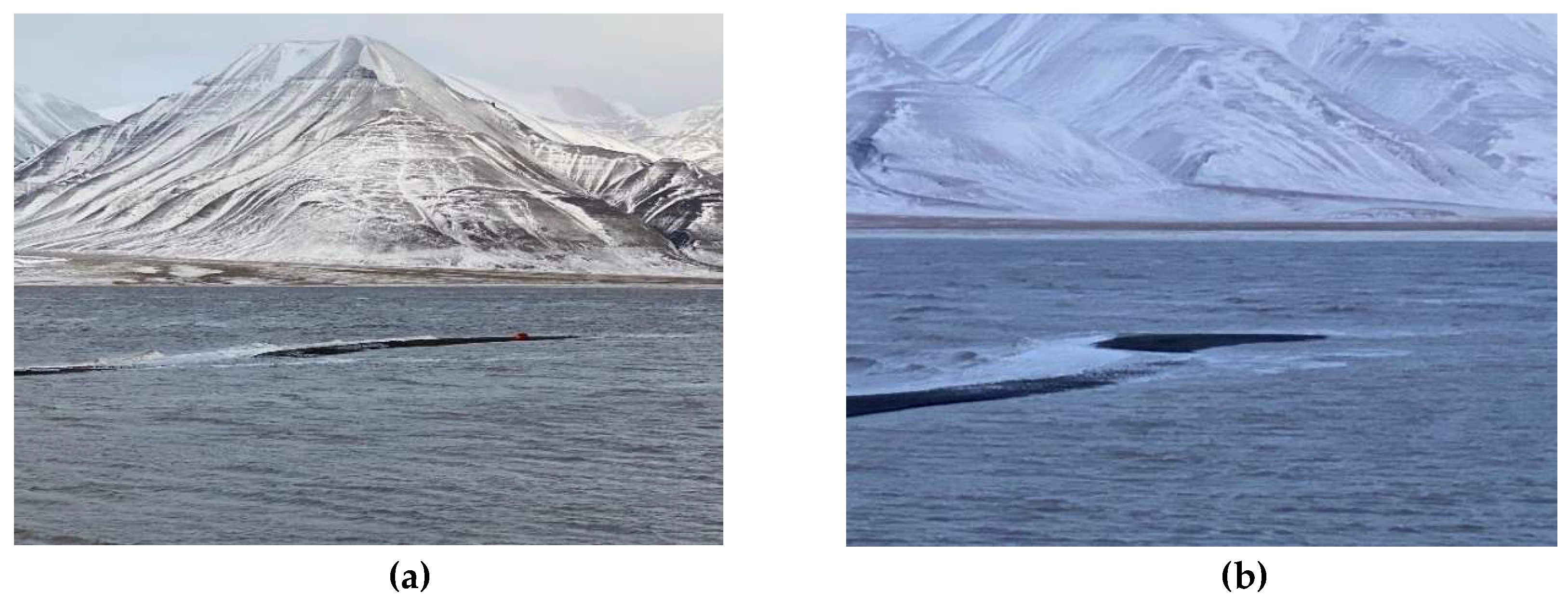
Figure 25.
Laser scans of the spit made at low tide phases on October 2 (a) and October 5 (b). Colorized by elevation (color bar on the right side on the picture is in Project Coordinate system). Over wash of the spit on October 2 (a) and October 5 (b), 2023.
Figure 25.
Laser scans of the spit made at low tide phases on October 2 (a) and October 5 (b). Colorized by elevation (color bar on the right side on the picture is in Project Coordinate system). Over wash of the spit on October 2 (a) and October 5 (b), 2023.
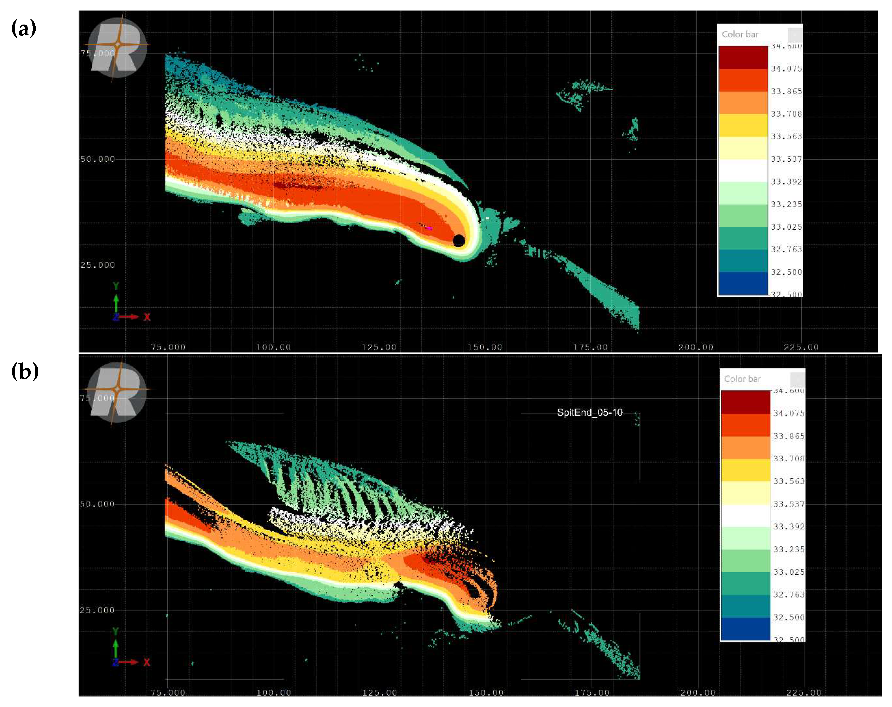

Table 1.
Dates of deployment of pressure and temperature recorders SBE 39 and acoustic Doppler velocimeter ADV in locations ADV-I, ADV-II, and ADV-III..
Table 1.
Dates of deployment of pressure and temperature recorders SBE 39 and acoustic Doppler velocimeter ADV in locations ADV-I, ADV-II, and ADV-III..
| Device | Measurement start | Measurement end |
| SBE1 | October 12, 2022 | August 6, 2023 |
| SBE2 | October 12, 2022 | October 23, 2022 |
| SBE3 | October 12, 2023 | June 17, 2023 |
| ADV-I | October 12, 2022 | October 23, 2022 |
| ADV-II | October 2, 2023 | October 3, 2023 |
| ADV-III | October 3, 2023 | October 4, 2023 |
Disclaimer/Publisher’s Note: The statements, opinions and data contained in all publications are solely those of the individual author(s) and contributor(s) and not of MDPI and/or the editor(s). MDPI and/or the editor(s) disclaim responsibility for any injury to people or property resulting from any ideas, methods, instructions or products referred to in the content. |
© 2025 by the authors. Licensee MDPI, Basel, Switzerland. This article is an open access article distributed under the terms and conditions of the Creative Commons Attribution (CC BY) license (http://creativecommons.org/licenses/by/4.0/).
Copyright: This open access article is published under a Creative Commons CC BY 4.0 license, which permit the free download, distribution, and reuse, provided that the author and preprint are cited in any reuse.


