1. Introduction
Electricity generation in Brazil is predominantly renewable, with more than 80% of the total generation capacity coming from renewable sources, primarily hydroelectric power, which constitutes over 65% of the country’s energy matrix [
1]. However, during droughts, which can severely impact water reservoirs, thermal power plants are needed to compensate for the shortfall, operating continuously at maximum capacity [
2]. To sustainably address this challenge, it is crucial to diversify into other renewable sources, such as wind energy, which can complement hydroelectric power [
3,
4].
Accurate modeling and forecasting of wind speed are crucial for effectively planning, operating, and monitoring electrical systems, especially in a complex grid like Brazil’s. Pinson (2013) highlights the importance of addressing the stochastic nature of renewable energy generation to enhance the robustness and reliability of energy systems. Effective stochastic modeling is vital for informed decision-making in both public and private sectors [
6].
Currently, the Brazilian electricity sector employs a Periodic Autoregressive (PAR) model [
7] to generate synthetic wind speed series correlated with hydroelectric reservoir inflows, based on the work of Maceira et al. (2022). While this model provides a foundation, it primarily considers wind speed in isolation and assumes that wind series are stationary, linear, and follow a Normal distribution [
8]. Furthermore, it does not incorporate exogenous variables that could influence wind regimes and energy production.
To improve the accuracy of wind energy forecasts, it is essential to integrate current climate variables, as wind energy generation is significantly affected by climate conditions, which can impact the availability and production of wind resources in Brazil [
9]. Incorporating climate variables into wind speed modeling can reduce forecasting uncertainties [
10,
11]. While common climate variables include pressure, temperature, and precipitation, the El Niño-Southern Oscillation (ENSO) phenomenon also shows a strong relationship with wind speed [
12,
13]. Notably, ENSO’s influence on wind speed has been documented in Brazil and globally [
14,
15,
16], supporting its use in forecasting models.
Moreover, Maçaira et al. (2018) have systematically reviewed various forecasting techniques, identifying regression models, neural networks, AutoRegressive Integrated Moving Average with Exogenous Variables (ARIMAX), support vector machines (SVM), and structural models as commonly used in studies incorporating exogenous variables. A more recent study by Pessanha et al. (2024) explored dynamic models combined with Bayesian approaches for generating wind speed time series, further advancing the field of wind speed forecasting.
This study introduces an advanced forecasting approach by extending the existing Periodic Autoregressive (PAR) model to incorporate Periodic Autoregressive models with Exogenous Variables (PARX) [
19,
20]. This innovative framework builds upon previous successful applications, such as Maçaira works on streamflow forecasting that uses a PAR that considers exogenous variables [
21,
22] and ARX models used on the wind and electricity [
23,
24]. By integrating climate variables like ENSO into the PARX framework, the proposed approach aims to enhance the modeling and forecasting capabilities for wind speed significantly, offering substantial improvements over current methods used in the Brazilian energy sector.
Furthermore, to enhance the understanding of wind speed patterns, variability, and trends, this study considers the spatial covariance between wind speeds across different states in Brazil. Previous research, such as that by Duran et al. (2007), demonstrated that aggregating forecasts from multiple wind farms can improve prediction accuracy. Additionally, Iung et al. (2023) conducted a comprehensive literature review highlighting various methods to quantify temporal dependence in renewable energy modeling, underscoring the importance of advanced forecasting techniques.
The primary objective of this research is to develop a methodology for forecasting wind speed, aiming to improve the accuracy of wind speed predictions and, consequently, wind power. Specifically, the study seeks to achieve the following secondary objectives: (i) integrate an exogenous variable into the PAR model by employing the Periodic Autoregressive model with Exogenous Variables (PARX); (ii) consider the covariance between wind regimes across states in each Brazilian region to enhance modeling precision; (iii) account for the correlation between ENSO phenomenon indicators to facilitate out-of-sample forecasting of climatic variables, and (iv) utilize these forecasts to simulate wind speed scenarios.
The work is organized into five sections. Following this introduction,
Section 2 will detail the applied methodology.
Section 3 will present a descriptive analysis of wind and climatic variables.
Section 4 will discuss the results and their implications, and
Section 5 will provide conclusions and discuss the research findings.
2. Methodology
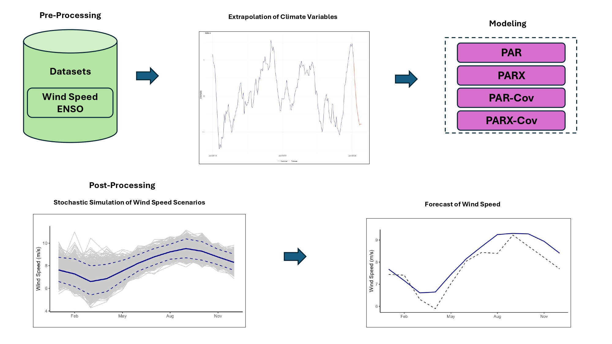
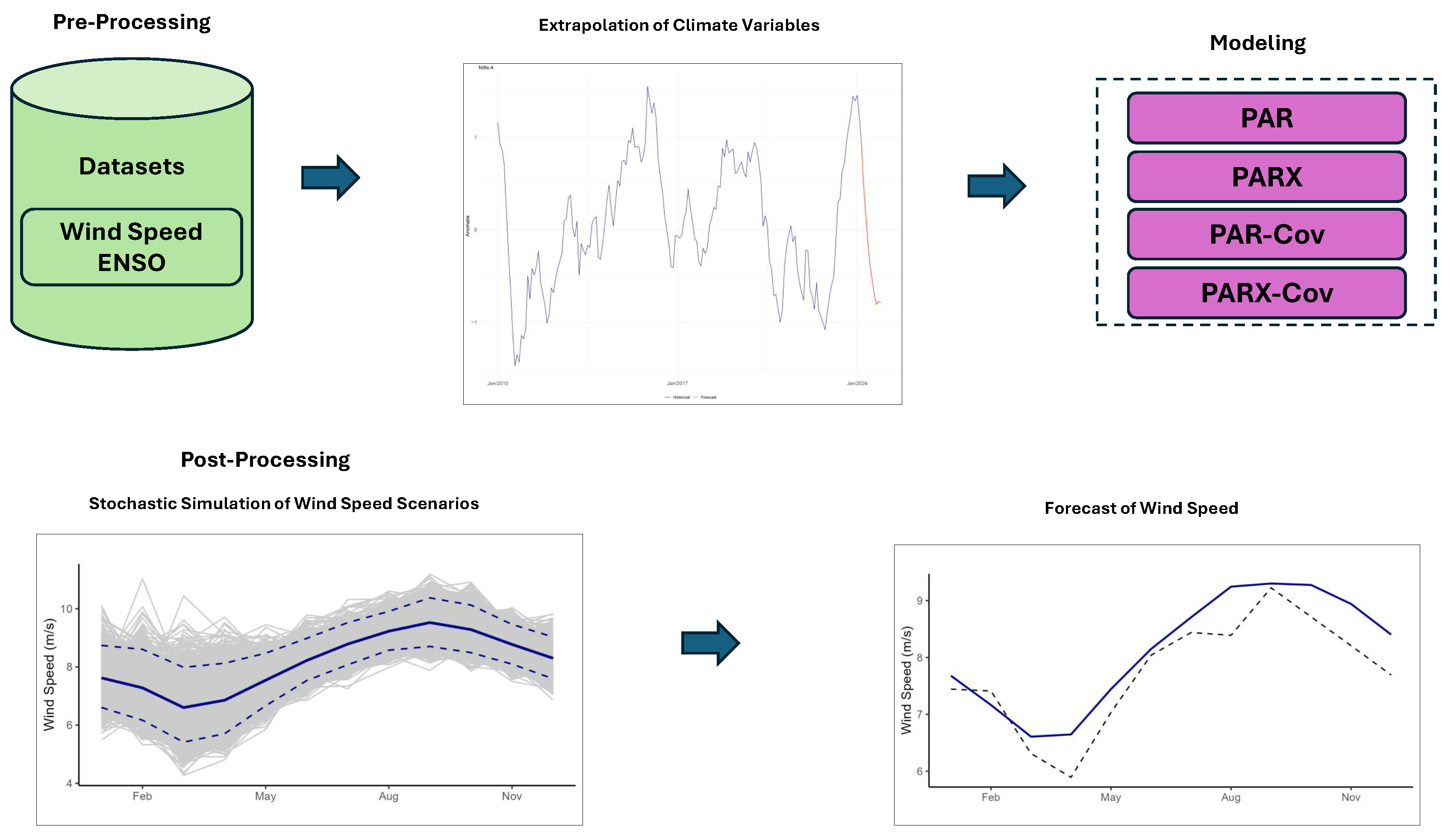
To summarize, the steps to achieve the objectives of this research can be observed through the methodological framework shown in
Figure 1.
2.1. Pre-Processing
2.1.1. Datasets
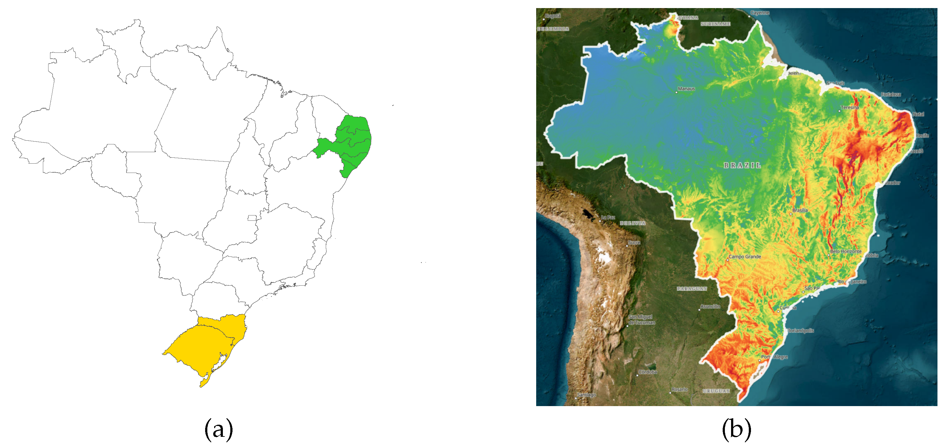
For the analyses conducted in this study, five states from the Northeast region were selected: Rio Grande do Norte (RN), Paraíba (PB), Pernambuco (PE), Alagoas (AL), and Sergipe (SE), along with two states from the South region: Rio Grande do Sul (RS) and Santa Catarina (SC). These states feature coastal areas with high wind power generation in Brazil, as highlighted in
Figure 2 in green for the Northeastern states and yellow for the Southern states, along with the wind potential for Brazil based on the Global Wind Atlas [
26], the redder it is, the greater the wind potential..
The MERRA-2 dataset is one of the most widely used reanalysis datasets in the literature for obtaining wind speed time series [
27,
28,
29]. In this context, the data used in this study were sourced from MERRA-2. Specifically, the data for the regions under study were collected using an automated script connected to the
Renewables.ninja website [
30], covering the period from January 1980 to December 2023 [
31,
32].
Renewables.ninja provides hourly data, and the script transforms this data into monthly aggregates. The coordinates for data collection were selected based on the Global Wind Atlas [
26] once more (
Figure 2). In each state, three points at an altitude of 100 meters above the surface were selected, which exhibited the highest wind speeds possible inside the state, not being far from each other (< 100 km) to ensure that the wind regimes were similar. Subsequently, the average of the time series of these three coordinates was calculated and used to represent the historical series of each state. It is worth noting that the choice of multiple points, rather than a single one, aimed to avoid data bias and provide better representativeness by covering a larger area.
Data on ENSO anomalies, where El Niño refers to the warming of Pacific Ocean waters and La Niña to cooling, were divided into two groups: historical and forecasted. Historical data were directly obtained from the Climate Prediction Center (CPC) of the National Oceanic and Atmospheric Administration (NOAA) [
33,
34], covering the period from 1931 to March 2024, with the initial date varying between ENSO indices. From this dataset, new variables were created: the first variable identifies ENSO periods classified as El Niño, La Niña, or Neutral; the others represent cumulative indices over time. This dataset is relevant for investigating trends in cumulative indices, which can indicate variations in sea pressure and temperature.
Forecast data were obtained from the International Research Institute (IRI), affiliated with NOAA [
35]. The IRI provides several models with a forecast horizon of up to 9 months for the ONI index. Two forecast periods were collected: the first from April 2023 to December 2023, aimed at improving fitting and prediction compared to using observed values alone; and the second from April 2024 to December 2024 for forecasting future out-of-sample scenarios [
35].
2.1.2. Extrapolation of Climate Variables
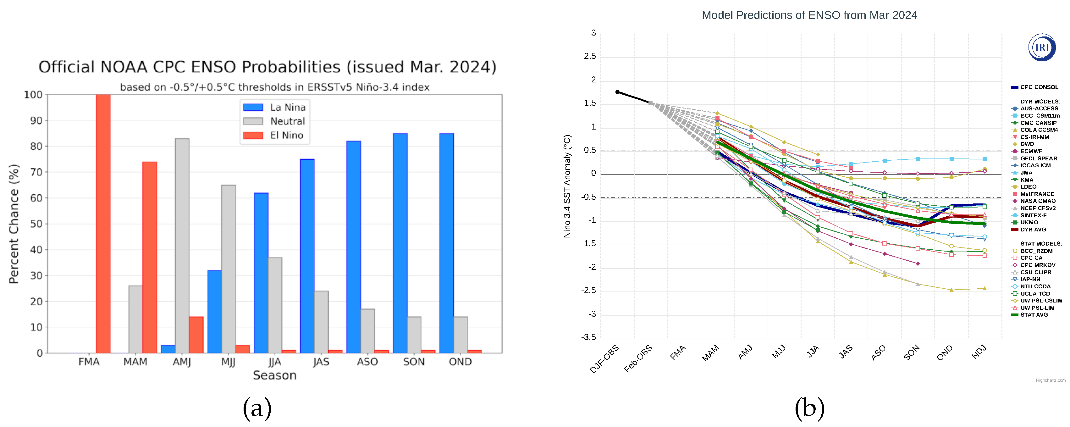
Official forecasts of ENSO phase probabilities by the CPC are based on a consensus among their meteorologists and the IRI. It is grounded in observational and predictive information from the beginning and previous months, meaning it incorporates analysis of various model outputs and human judgment. Models applied by the IRI generate forecasts of ENSO anomalies and are divided into two groups: dynamic and statistical, in addition to their ensemble mean. The NOAA CPC consolidated model averages certain models [
35].
In
Figure 3, it can be seen that the forecasts suggest a transition from El Niño to La Niña in 2024, highlighted by the Phase Probabilities. The Anomalies also reflect a sharp decline in the ONI index anomalies.
The average of anomalies from all ONI index models is also provided and will be used in this work. To obtain the forecast of anomalies for other indices, which are not provided by the IRI, a linear regression will be applied [
36,
37].
2.2. Modeling
2.2.1. Periodic Autoregressive Model (PAR)
According to Hipel & McLeod (1994), the PAR model is an approach used for modeling seasonal time series. When fitting a PAR model to a seasonal series, an individual Autoregressive (AR) model is applied to each recurring period of the seasonality. For example, in a monthly seasonal series, the PAR model is configured so that each month has its own AR model, allowing for more precise capture of specific variations within each period over time. PAR is also denoted as PAR(p), where p represents the order of the model.
Following the notation commonly used when referring to the PAR model, let
Z be a series with
S periods and
N number of years, then
. The PAR model of series
Z in period
m is mathematically described by Equation
1.
where
is the mean of period
m,
is the standard deviation of period
m,
is the
i-th autoregressive coefficient of period
m,
is the order of the autoregressive operator of period
m, and
is the series of independent noises with mean 0 and standard deviation
. In the specific case of January (
), the model will be applied to December of the previous year, i.e., to the period (
), where it is assumed that December is represented by
.
To select the autoregressive order for each month, the Bayesian Information Criterion (BIC) will be used, as it is effective for simpler models and selection within a group. The order with the lowest BIC will be chosen for each period in the wind speed series of the PAR model [
39,
40,
41].
After determining the model order, it is necessary to estimate the parameters
. Let
be the vector of autoregressive parameters for period
m. An asymptotically efficient estimator,
, can be obtained by solving Equations
3 using Ordinary Least Squares (OLS) [
42].
2.2.2. Periodic Autoregressive Model with Exogenous Variables (PARX)
The Periodic Autoregressive model with Exogenous Variables (PARX) is an extension of the PAR model. In addition to the seasonal autoregressive structure, it incorporates an additional explanatory variable denoted by
X. This auxiliary variable,
X, allows the model to consider and capture the effects and influences of this variable on the seasonal time series, providing a more comprehensive analysis and potentially improving forecasting capabilities by accounting for external factors that impact the seasonality of the series [
19,
20].
Let
Z be the previously defined periodic series and
X be the exogenous variable in the modeling of
Z, with the same number of observations (
) and periodicity (
S) as
Z. According to Ursu & Pereau (2017) and Silveira et al. (2017), the PARX for the dependent variable
Z and the exogenous variable
X can be mathematically expressed as follows:
where
is the mean of the dependent variable
Z for the period
m,
is the standard deviation of the dependent variable
Z for the period
m,
is the
i-th autoregressive coefficient of the dependent variable
Z for period
m,
is the order of the autoregressive operator of the dependent variable
Z for period
m.
is the mean of the independent variable
X for period
m,
is the standard deviation of
X for period
m,
is the
j-th autoregressive coefficient of the exogenous variable
X for period
m,
is the order of the autoregressive operator of the exogenous variable
X for the period
m, and
is the series of independent noises with mean 0 and standard deviation
. In the particular case of January (
), a similar approach to the PAR model is applied. The model utilizes December of the previous year, referring to the instant (
), where it is considered that the period of December is represented by
.
To determine the autoregressive orders of the dependent variable and the exogenous variable for each period (
,
), the BIC criterion will be employed again. In the context of the PARX model, for each period, the obtained BIC will be associated with the set (
,
). In other words, the set of parameters that results in the lowest BIC value will be selected as the most suitable for the model [
39,
40].
The parameter estimation for the model, similar to the PAR model, is performed via OLS [
19]. Let
and
, where
and
, with size
. Let
and
be vectors of dimension
, with
T being the transpose operator, and
the matrix with dimension
, where
and
are described by
Let
be the parametric vector, where
Given that Equation
4 is a linear model, it can be written in the form of a regression model:
The covariance matrix of the random vector
is
, where
is the identity matrix of size
N. The ordinary least squares estimator of
is obtained by minimizing Equation
9.
Finally, applying the difference operator to Equation
9 yields the least squares estimators
.
2.2.3. Covariance (PAR-Cov & PARX-Cov)
Given the modeling of the PAR and PARX models above, the correlation will act on their residuals. The concept of covariance will be introduced among the states in each Brazilian region, aiming to enhance modeling accuracy and simulation. This methodology will assess the relationship between wind speeds at different points within a given space, specifically in the Brazilian states under study. Moreover, considering covariance aims to improve the understanding of wind speed data by identifying patterns, variability, and trends [
43,
44].
This methodology can be approached through the following steps:
- 1.
Calculation of the Covariance Matrix
- 2.
Spectral Decomposition
- 3.
Multivariate Normal Distribution
Thus, two new models are developed: the PAR-Cov model and the PARX-Cov model.
2.3. Post-Processing
2.3.1. Performance Metrics
This study employs three widely used performance evaluation metrics to assess the accuracy of wind models in Brazil [
45,
46] and in the world [
41,
47]: Root Mean Square Error (RMSE) and Mean Absolute Error (MAE), both measures of error, and the Coefficient of Determination (
), a measure of model fitting, given by
where
represents the observed wind speed at time
t,
is the wind speed predicted by the model at the same time,
denotes the observed mean, and
T is the forecast horizon length.
2.3.2. Stochastic Simulation of Wind Speed Scenarios
After selecting the most appropriate models, synthetic scenarios for wind speed will be created through stochastic simulation. The goal is to reproduce stochastic behavior and generate new time series synthetically from one of the adjusted models: PAR, PAR-Cov, PARX, or PARX-Cov, based on the original series. These series will be distinct from the original historical data but equally plausible from a statistical perspective.
The established strategy for generating synthetic series involves fitting a three-parame-
ter Lognormal distribution to the monthly residuals (
) of the PAR model, for two main reasons [
7]. The first reason is to ensure that values are always positive, given the nature of wind data. The second reason stems from the strong asymmetry present in the data (and residuals), making the use of a Normal distribution impractical.
Firstly, Equation
1 of the PAR model is manipulated to isolate
:
Thus, to ensure that negative values of
are not generated:
Therefore, the variable
is a function of only the moments (mean and variance) of the period
m and the autoregressive coefficients, and is given by
Defining
and
as the mean and standard deviation, respectively, of the residual series of period
m (
), we have that:
Since these are random noises:
The parameters
and
are estimated in order to preserve the moments of the residuals, as per Charbeneau [
48] and reproduced by Pereira et al. [
49].
By manipulating the PARX model equations in the same way, it is possible to determine its own isolated
and
, as shown in the Equations ahead.
Furthermore, the equations for the PAR-Cov and PARX-Cov models are similar to their respective models but with the incorporation of covariance.
The Lognormal simulation method has residual nonlinearity limitations, as noted by Oliveira et al. [
7], who suggest using Bootstrap to address this. This study focuses on proposing superior modeling methods, keeping the current scenario generation technique to ensure improvements come from the proposed models.
2.3.3. Forecast of Wind Speed
Finally, it is possible to make a forecast from the created scenarios
h steps ahead. Next, the process is presented for the PAR methodology. First,
K scenarios are generated
h steps ahead, which was already presented in the previous subsection: (
Section 2.3.2):
for
.
Then the average of these scenarios is calculated to arrive at the forecast
:
For the PARX methodology, the forecast process is also show based the on the previous subsection (
Section 2.3.2):
for
.
Moreover, the PAR-Cov and PARX-Cov forecasting methods resemble their respective models, with the addition of covariance integration.
3. Descriptive Analysis of the Data
This section conducts a descriptive analysis of wind speed data and ENSO, as well as the relationship between them. All the analyses were performed here, and the results were obtained using the R software version of December 2022 [
50].
3.1. Wind Speed
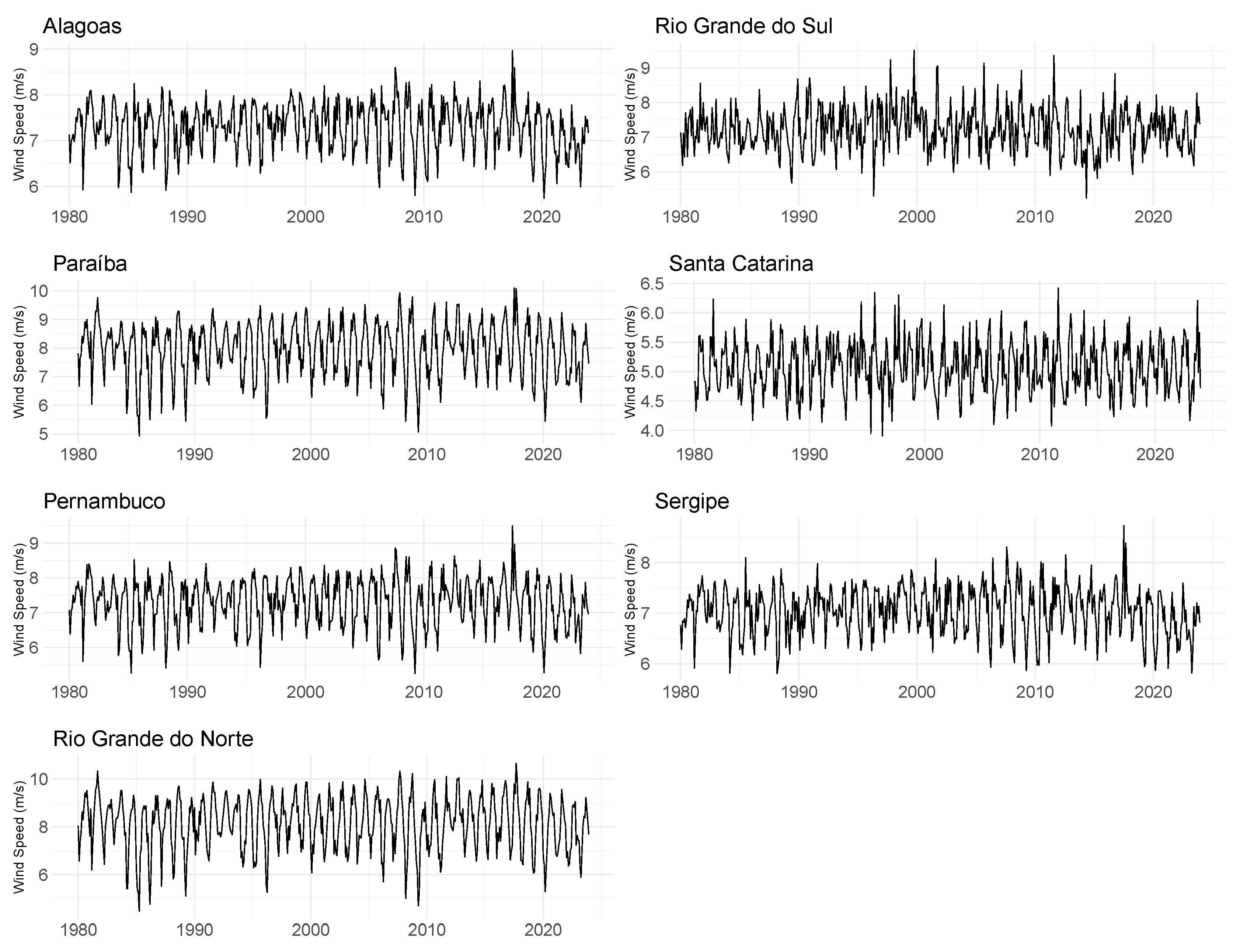
Initially, after wind speed data is collected from the MERRA-2 database, as mentioned in
Section 2.1.1,
Figure 4 shows the monthly time series for the states of Rio Grande do Norte (RN), Paraíba (PB), Pernambuco (PE), Alagoas (AL), Sergipe (SE), Rio Grande do Sul (RS), and Santa Catarina (SC) from January 1980 to December 2023. Observing the graphs, it is noticeable that overall, the states exhibit a well-defined seasonal behavior, with a particular emphasis on RN, PB, PE, AL, and SE located in the Northeast. It’s important to emphasize that it was not necessary to perform any kind of data cleaning.
It is also important to analyze the descriptive statistics of the time series, shown in
Table 1. Regarding measures of central tendency, there is close proximity between the mean and median values for the states. In this regard, the highest means are observed, as expected, in Rio Grande do Norte (
m/s) and Paraíba (
m/s) in the Northeast, while the lowest mean is observed in Santa Catarina (
m/s). Similarly, concerning standard deviation and coefficient of variation, Rio Grande do Norte and Paraíba also exhibit the highest measures. As for skewness, all values fall within the interval
, typical of distributions with slight skewness. Regarding kurtosis, it is noted that the states exhibit kurtosis around three, indicating that these distributions have a frequency curve close to the normal distribution.
To verify the stationarity of the series, the Augmented Dickey-Fuller (ADF) [
51] and Phillips-Perron tests [
52] were applied. Since all p-values are below a significance level of 5%, there is sufficient statistical evidence to reject the null hypothesis of non-stationarity for all states.
3.2. ENSO
ENSO indicators are located in various regions, each with specific significance [
53]. The Southern Oscillation Index (SOI) is one of the oldest, based on the sea level atmospheric pressure difference between Tahiti and Darwin. However, SOI is sensitive to short-term fluctuations and is limited by its location south of the Equator, while ENSO centers closer to the Equator. The Equatorial SOI addresses this by measuring pressure differences directly along the Equator between Indonesia and the Eastern Pacific.
In 1969, Bjerknes identified Sea Surface Temperature (SST) in the equatorial Pacific as a primary ENSO indicator [
54]. Initially, regions like Niño 1+2, Niño 3, and Niño 4 were used for measurements. Later, Niño 3.4 was deemed the most representative [
55], and its temperature anomaly is measured by the Oceanic Niño Index (ONI), which removes regional warming trends. ENSO events are identified through anomaly time series of indices, with ONI employing a three-month moving average.
For SOI, La Niña occurs with five consecutive months of positive indices above 0.5°C, while El Niño corresponds to five consecutive months of negative indices below -0.5°C. For SST, the reverse applies: El Niño corresponds to positive anomalies, and La Niña to negative ones [
33].
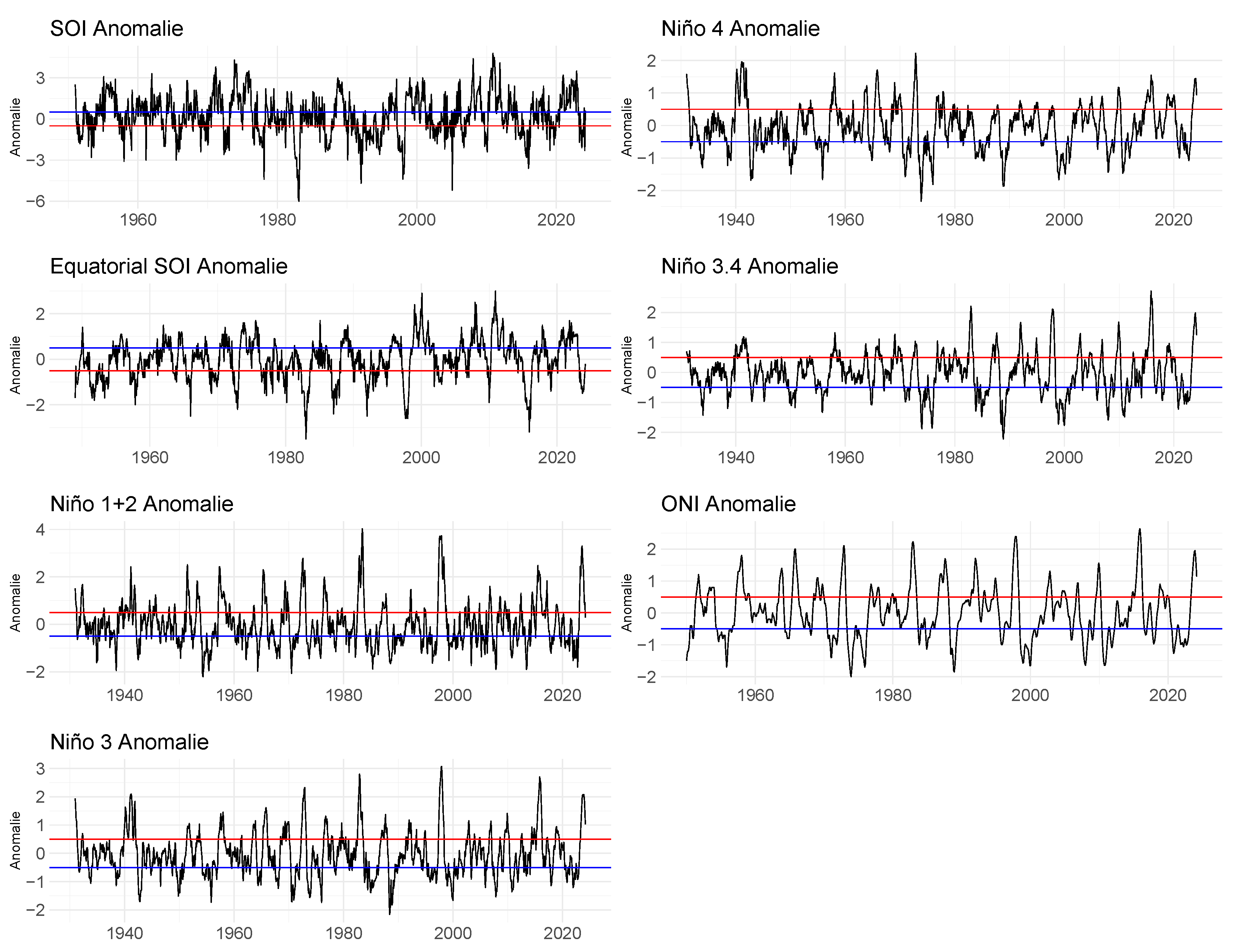
3.2.1. Historical
Graphs for all ENSO indices are shown in
Figure 5, presenting monthly historical data from 1931 to March 2024, with the start date varying according to each ENSO index. Regarding the SOI indices, sequences above the blue line indicate La Niña events, and sequences below the red line indicate El Niño events. For SST and ONI indices, sequences of points above the red line indicate El Niño events, while sequences below the blue line indicate La Niña events.
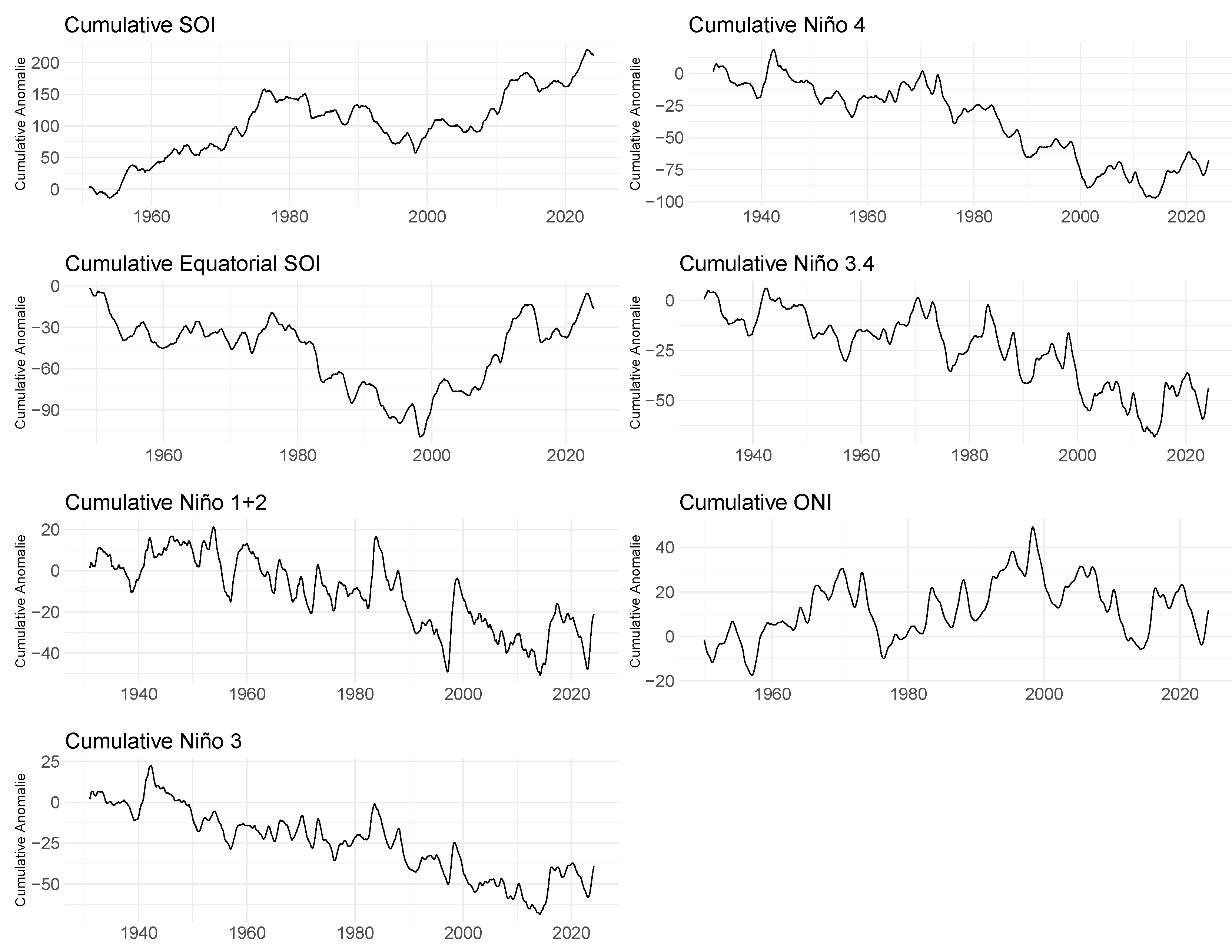
Cumulative series can be observed in
Figure 6, showing that according to the SOI and Equatorial SOI indices, there is a trend of increasing sea level atmospheric pressure both between the regions of Taiti and Darwin, as well as between Indonesia and the Eastern Pacific in recent years. Also, in
Figure 6, cumulative indices for SST and ONI are presented. Note that after 1980, all these indices except ONI show a downward trend.
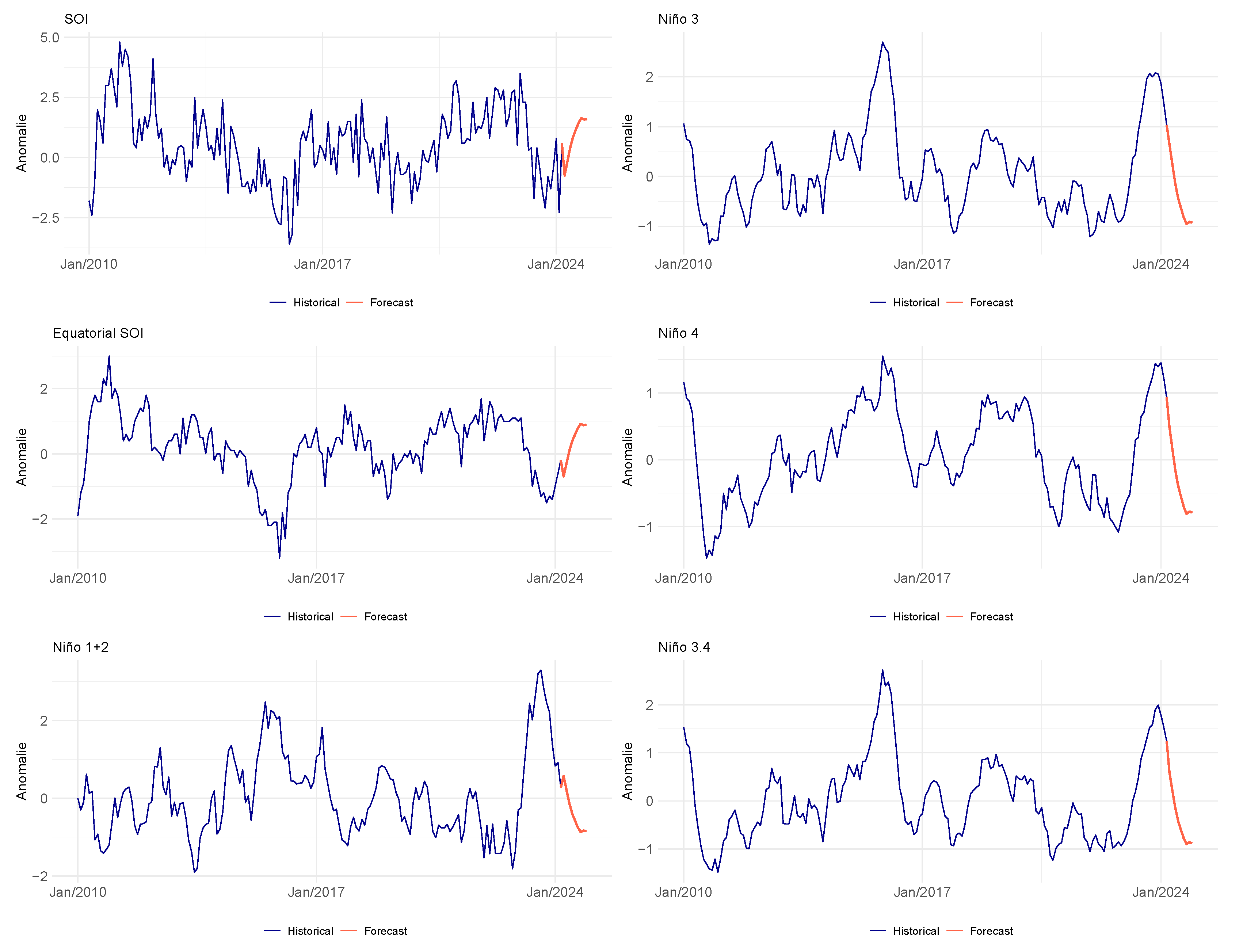
3.2.2. Forecast
The forecast of the ONI index from April 2024 to December 2024 will be used to assist in predicting future wind speed scenarios, as mentioned in
Section 2.1.1. This forecast will be analyzed below obtaining the forecast of anomalies for other the indices of ONI, which are not provided by the IRI. For this purpose, the linear regression will be applied [
36,
37]..
Firstly, an fit was made between the observed data for each index and the ONI. The regression results can be seen in
Table 2. The results show that the indices that obtained the best adjustments were Niño 3.4 and Niño 3 with R² values of 0.882 and 0.831, respectively. Furthermore, the sign of the coefficients reflects the relationship of each index with ONI, with the SOI and Equatorial SOI having a negative correlation, while the SST indices have a positive correlation.
From this, it is possible to construct the forecast of indices based on ONI. In
Figure 7, these forecasts are shown in red, alongside their histories since 2010, shown in blue.
3.3. Relationship Between Wind Speed and ENSO
One of the hypotheses of this study is that the ENSO may impact wind speeds. To assess differences in wind speed distributions based on ENSO phases (El Niño, La Niña, or neutral periods), a Kruskal-Wallis test was performed. This test compares multiple independent groups using a quantitative response variable and can handle groups of different sizes. Importantly, it does not assume normality or equal variances. The tested hypotheses are:
: The k samples come from the same population.
: At least one of the samples comes from a population different from the others.
When evaluating the test in
Table 3, a significance level of 10% was chosen. If the wind speed in the phases has the same distribution, the answer is “Yes”, meaning that the null hypothesis is not rejected. If the phases do not have the same distribution, the answer is “No”, indicating that the null hypothesis is rejected.
It is evident that all states, with the exception of Alagoas, exhibit at least one index that confirms distinct distributions between the ENSO phases. Therefore, it is statistically proven that the ENSO climatic phenomenon can influence wind speed patterns in the areas under study.
4. Results
Initially, the proposed models will be evaluated based on their forecasting accuracy, generating wind speed scenarios using the selected model. To assess the performance of each model, the dataset was divided into seven fitting and forecasting windows, as detailed in
Table 4.
In window 1, the selection of parameters and will be determined for the PARX and PARX-Cov models. For each state and each parameter combination, the following steps will be executed, considering exclusively the first window:
- i)
Fit the wind speed series for the in-sample period;
- ii)
Simulate scenarios of the out-of-sample period (using the observed values of climatic variables from the in-sample period);
- iii)
Compare the forecasted values, calculated as the average of the scenarios, with the observed value;
- iv)
Record the errors obtained.
The parameters selected for each state and model will result in the smallest error. These parameters will be applied to windows 2 to 5 to calculate performance metrics, following the procedures from window 1 but focusing exclusively on the best combination identified initially. The error and adjustment values presented in this section are averaged across the four windows (2 to 5) to more robustly evaluate the predictive capability of the models using the RMSE, MAE, and metrics. Based on these results, the best models for each state will be selected.
Once the best models have been identified, they will be applied to window 6, using the ENSO forecast for 2023, obtained similarly to the process used for the 2024 period. Finally, in window 7, forecasts for future scenarios in 2024 will be made, also utilizing out-of-sample ENSO data based on the previously identified best models.
It is important to note that models with accumulated indices will be referred to as ’CUM’ along with the name of the corresponding index to be abbreviated.
Table 5 highlights the models with the best performance according to the RMSE, MAE, and
metrics, including improvements over the PAR model. It is important to note regarding the RMSE metric that the states with the largest improvements were Rio Grande do Sul (2.87%) and Santa Catarina (2.65%), using PARX-Cov models. On the other hand, the state of Pernambuco recorded the smallest improvement (0.87%), although it still showed an advantage over the PAR model. For the MAE metric, the largest improvement came once again from the South Region, with a 4.47% increase for Santa Catarina using a PARX-Cov model. Notably, Paraíba also showed a 2.19% improvement with a PARX model. Finally, the
metric reveals a small gain for the state of Rio Grande do Norte (0.71%), while Rio Grande do Sul demonstrated a significant gain of 19.29% using a PARX-Cov model.
Table 6 summarizes the models highlighted as the best, considering the three performance metrics for each of the seven states, resulting in 21 possible cases. It is observed that all the selected models incorporate the exogenous variable ENSO in the modeling, indicating its significant contribution, with the ONI index being the most prevalent, with 16 occurrences. Additionally, it is noted that 9 of the models are PARX-Cov, highlighting the importance of including covariance.
Considering the three performance metrics evaluated in
Table 5, the best model for each state was selected based on most metrics indicating that model as the best. The exception was the state of Pernambuco, where each metric pointed to a different model as the best; in this case, the metric indicating the greatest improvement was chosen. The selected best models are presented in
Table 7.
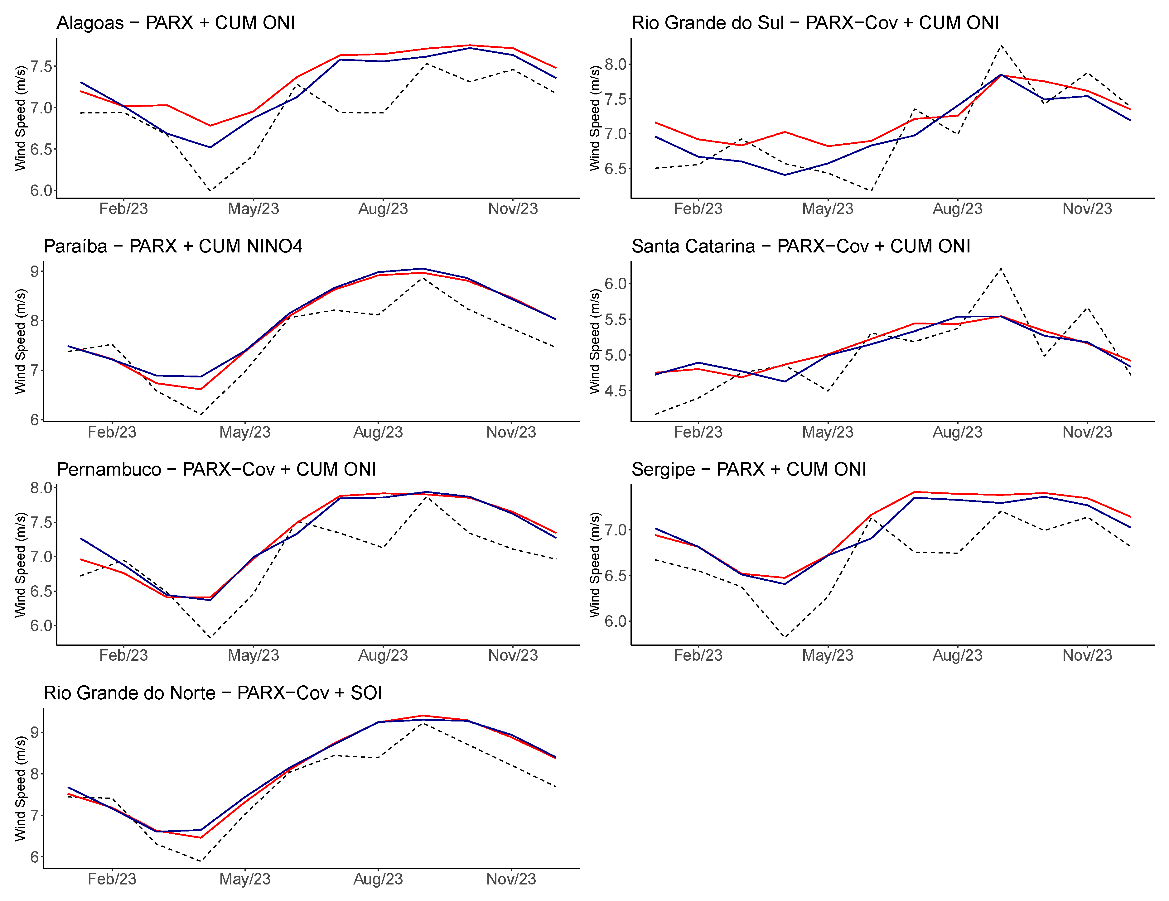
Finally, in
Figure 8, the observed wind speeds during the validation period of window 6 (Jan/2023-Dec/2023) are depicted in black. Forecasts obtained using the PAR model are shown in red, while forecasts from the best PARX or PARX-Cov models for each state are highlighted in dark blue.
As seen in
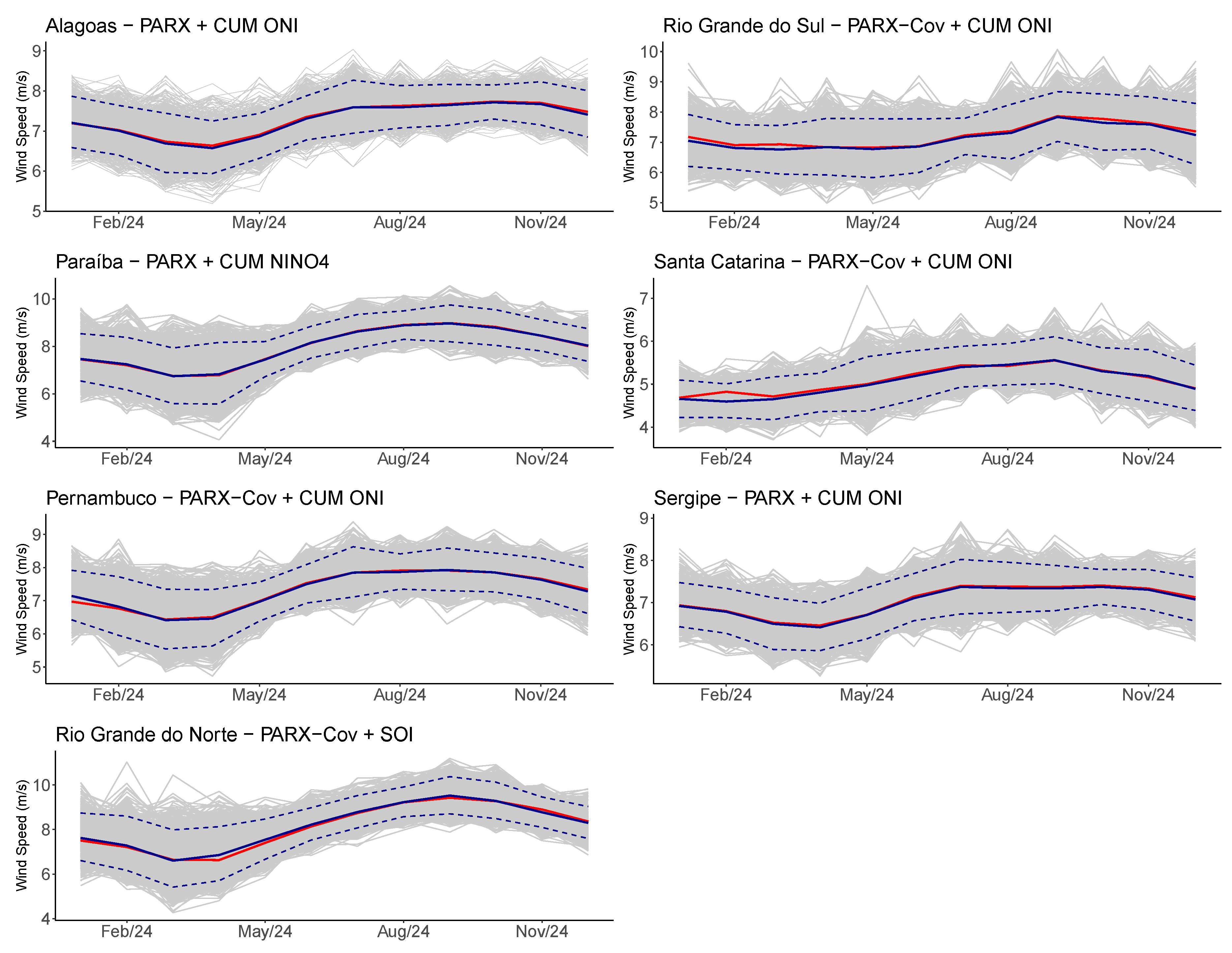
Figure 3, it is expected that 2024 will see a transition from El Niño to La Niña, with a sharp decline in ONI index anomalies. Therefore, in
Figure 9, scenarios (grey) with percentile 5% and 95% (dashed dark blue), and forecasts for window 7 (Jan/2024-Dec/2024) are presented for each state. These forecasts were obtained using the best PARX or PARX-Cov model (dark blue), which incorporates the out-of-sample ENSO climatic variable, and the PAR model (benchmark), in red.
5. Conclusion
Given the substantial expansion of wind energy in Brazil as a response to current climate change (IRENA), this study presents a methodological approach aimed at integrating climatic variables to enhance the modeling and forecasting of wind speed, thereby contributing to reducing uncertainties in the electricity sector. The proposed method involves incorporating an explanatory variable into the Periodic Autoregressive (PAR) model for wind speed series, which is currently utilized in the Brazilian electricity sector (Maceira, 2022). This incorporation is achieved through the application of the Periodic Autoregressive model with Exogenous Variables (PARX), including the exogenous variable ENSO. The model saw application to wind speed reanalysis data from coastal regions noted for high wind generation, encompassing five states in the Northeast (Rio Grande do Norte, Paraíba, Pernambuco, Alagoas, and Sergipe) and two states in the South (Rio Grande do Sul and Santa Catarina).
To enhance the accuracy of modeling and forecasting efforts, the paper introduces the concept of incorporating covariance between these states in each Brazilian region. Spatial correlation analysis emerges as crucial in understanding the interconnections, thereby adding an additional dimension to the methodological approach and resulting in the creation of the PAR-Cov and PARX-Cov models. Additionally, nine-month forecasts of the ENSO phenomenon (ONI) were collected, alongside an approach developed to enable out-of-sample forecasting of other climatic variables. This was aimed at achieving better adjustment and prediction than would be possible using observed values alone. Finally, out-of-sample forecasts of climatic variables were employed to forecast wind speed scenarios, importantly ensuring the absence of negative values.
Compared to the existing PAR model, the proposed models show superior performance in modeling wind speed series. This indicates that the inclusion of covariance and climatic variables significantly impacts wind speed across the analyzed Brazilian states, thereby directly affecting the country’s energy generation capacity. Analysis of the models concludes that PARX-Cov with Cumulative ONI is most suitable for three states: Pernambuco, Rio Grande do Sul, and Santa Catarina. In contrast, PARX-Cov with the SOI index is more fitting for Rio Grande do Norte. Further, PARX with Cumulative ONI is advised for Alagoas and Sergipe, while PARX with Cumulative Niño 4 is recommended for Paraíba.
As a continuation, the application of advanced statistical models is proposed to tackle the nonlinear aspects of wind speed time series and to model the non-Gaussianity of the data, often demonstrated by extreme events. It is also important to expand the study to encompass other states in the Northeast, noted for being major energy producers, along with offshores places. Analysis could be conducted for the Northeast subsystem or by distinguishing between interior and coastal regions. Lastly, it is suggested to convert wind speed into energy generation estimates and integrate this proposed modeling into an optimization program for energy operation, such as PDDE or NEWAVE.
Author Contributions
Conceptualization, Rafael Couto, Paula Maçaira and Fernando Cyrino; Data curation, Rafael Couto; Formal analysis, Rafael Couto; Investigation, Rafael Couto; Methodology, Rafael Couto; Resources, Paula Maçaira and Fernando Cyrino; Software, Rafael Couto and Paula Maçaira; Supervision, Paula Maçaira and Fernando Cyrino; Validation, Paula Maçaira and Fernando Cyrino; Visualization, Rafael Couto; Writing – original draft, Rafael Couto; Writing – review & editing, Paula Maçaira and Fernando Cyrino.
Funding
This work was partially supported by Rio Paraná Energia S.A. through RD project ANEEL PD-10381-0322/2022, CAPES Finance Code 001, CNPq (422470/2021-0, 307084/2022-1, 311519/2022-9, 402971/2023-0) and FAPERJ (210.618/2019, 211.086/2019, 211.645/2021, 201.243/2022, 201.348/2022, 210.041/2023, 210.015/2024).
Data Availability Statement
References
- EPE. https://www.epe.gov.br/pt/publicacoes-dadosabertos/publicacoes/balanco-energetico-nacional-ben, 2021. Accessed: 10-05-2023.
- Rigotti, J.A.; Carvalho, J.M.; Soares, L.M.; Barbosa, C.C.; Pereira, A.R.; Duarte, B.P.; Mannich, M.; Koide, S.; Bleninger, T.; Martins, J.R. Effects of hydrological drought periods on thermal stability of Brazilian reservoirs. Water 2023, 15, 2877. [CrossRef]
- Maceira, M.; Melo, A.; Pessanha, J.; Cruz, C.; Almeida, V.; Justino, T. Wind Uncertainty Modeling in Long-Term Operation Planning of Hydro-Dominated Systems. In Proceedings of the 2022 17th International Conference on Probabilistic Methods Applied to Power Systems (PMAPS). IEEE, 2022, pp. 1–6.
- Melo, G.; Barcellos, T.; Ribeiro, R.; Couto, R.; Gusmão, B.; Oliveira, F.L.C.; Maçaira, P.; Fanzeres, B.; Souza, R.C.; Bet, O. Renewable energy sources spatio-temporal scenarios simulation under influence of climatic phenomena. Electric Power Systems Research 2024, 235, 110725. [CrossRef]
- Pinson, P. Wind energy: Forecasting challenges for its operational management. Statistical Science 2013. [CrossRef]
- Ferreira, P.G.C.; Oliveira, F.L.C.; Souza, R.C. The stochastic effects on the Brazilian Electrical Sector. Energy Economics 2015, 49, 328–335. [CrossRef]
- Souza, R.C.; Marcato, A.; Dias, B.H.; Oliveira, F.L.C.; et al. Optimal operation of hydrothermal systems with hydrological scenario generation through bootstrap and periodic autoregressive models. European Journal of Operational Research 2012, 222, 606–615. [CrossRef]
- Noakes, D.; McLeod, A.; Hipel, K. Forecasting monthly riverflow time series. International Journal of Forecasting 1985, 1, 179–190. https://doi.org/10.1016/0169-2070(85)90022-6. [CrossRef]
- EPE. Plano Nacional de Energia - PNE 2050. https://static.poder360.com.br/2020/12/PNE2050.pdf, 2018. Accessed: 20-05-2022.
- do Nascimento Camelo, H.; Lucio, P.S.; Junior, J.B.V.L.; de Carvalho, P.C.M. A hybrid model based on time series models and neural network for forecasting wind speed in the Brazilian northeast region. Sustainable Energy Technologies and Assessments 2018, 28, 65–72. [CrossRef]
- de Mattos Neto, P.S.; de Oliveira, J.F.; Júnior, D.S.d.O.S.; Siqueira, H.V.; Marinho, M.H.; Madeiro, F. An adaptive hybrid system using deep learning for wind speed forecasting. Information Sciences 2021, 581, 495–514. [CrossRef]
- Corrêa, C.S.; Schuch, D.A.; Queiroz, A.P.d.; Fisch, G.; Corrêa, F.d.N.; Coutinho, M.M. The long-range memory and the fractal dimension: A case study for Alcântara. Journal of Aerospace Technology and Management 2017, 9, 461–468. [CrossRef]
- Lima, C.N.N.; Fernandes, C.A.C.; França, G.B.; de Matos, G.G. Estimation of the El Niño/La Niña Impact in the Intensity of Brazilian Northeastern Winds. Anuário do Instituto de Geociências 2014, 37, 232–240.
- Arpe, K.; Molavi-Arabshahi, M.; Leroy, S.A.G. Wind variability over the Caspian Sea, its impact on Caspian seawater level and link with ENSO. International Journal of Climatology 2020, 40, 6039–6054. [CrossRef]
- Xu, Q.; Li, Y.; Cheng, Y.; Ye, X.; Zhang, Z. Impacts of Climate Oscillation on Offshore Wind Resources in China Seas. Remote Sensing 2022, 14, 1879. [CrossRef]
- Coria-Monter, E.; Salas de León, D.A.; Monreal-Gómez, M.A.; Durán-Campos, E. Satellite observations of the effect of the “Godzilla El Niño” on the Tehuantepec upwelling system in the Mexican Pacific. Helgoland Marine Research 2019, 73, 1–11.
- Maçaira, P.; Thomé, A.; Cyrino Oliveira, F.; de Almeida, F. Time series analysis with explanatory variables: A systematic literature review. Environmental Modelling & Software 2018, 107, 199––209. [CrossRef]
- de Mendonça, M.J.C.; Pessanha, J.F.M.; de Almeida, V.A.; Medrano, L.A.T.; Hunt, J.D.; Junior, A.O.P.; Nogueira, E.C. Synthetic wind speed time series generation by dynamic factor model. Renewable Energy 2024, 228, 120591. [CrossRef]
- Ursu, E.; Pereau, J. Estimation and identification of periodic autoregressive models with one exogenous variable. Journal of the Korean Statistical Society 2017, 46, 629–640. [CrossRef]
- Silveira, C.; Alexandre, A.; de Souza Filho, F.; Vasconcelos Junior, F.; Cabral, S. Monthly streamflow forecast for National Interconnected System (NIS) using Periodic Auto-regressive Endogenous Models (PAR) and Exogenous (PARX) with climate information. Brazilian Journal of Water Resources 2017, 22. https://doi.org/10.1590/2318-0331.011715186. [CrossRef]
- Maçaira, P.M.; Oliveira, F.L.C.; Ferreira, P.G.C.; Almeida, F.V.N.d.; Souza, R.C. Introducing a causal PAR (p) model to evaluate the influence of climate variables in reservoir inflows: A Brazilian case. Pesquisa Operacional 2017, 37, 107–128. [CrossRef]
- Huang, X.; Maçaira, P.M.; Hassani, H.; Oliveira, F.L.C.; Dhesi, G. Hydrological natural inflow and climate variables: Time and frequency causality analysis. Physica A: Statistical Mechanics and its Applications 2019, 516, 480–495. [CrossRef]
- Duran, M.J.; Cros, D.; Riquelme, J. Short-term wind power forecast based on ARX models. Journal of Energy Engineering 2007, 133, 172–180. [CrossRef]
- Golia, S.; Grossi, L.; Pelagatti, M. Machine Learning Models and Intra-Daily Market Information for the Prediction of Italian Electricity Prices. Forecasting 2022, 5, 81–101. [CrossRef]
- Iung, A.M.; Cyrino Oliveira, F.L.; Marcato, A.L.M. A review on modeling variable renewable energy: Complementarity and spatial–temporal dependence. Energies 2023, 16, 1013. [CrossRef]
- Atlas, G.W. Available at: https://globalwindatlas.info/en. Accessed on: November 27, 2023.
- de Aquino Ferreira, S.C.; Oliveira, F.L.C.; Maçaira, P.M. Validation of the representativeness of wind speed time series obtained from reanalysis data for Brazilian territory. Energy 2022, 258, 124746. [CrossRef]
- Gruber, K.; Klöckl, C.; Regner, P.; Baumgartner, J.; Schmidt, J. Assessing the Global Wind Atlas and local measurements for bias correction of wind power generation simulated from MERRA-2 in Brazil. Energy 2019, 189, 116212. [CrossRef]
- Olauson, J.; Bergkvist, M. Modelling the Swedish wind power production using MERRA reanalysis data. Renewable Energy 2015, 76, 717–725. [CrossRef]
- Renewables.ninja. Available at: https://www.renewables.ninja/. Accessed on: November 27, 2023.
- Pfenninger, S.; Staffell, I. Long-term patterns of European PV output using 30 years of validated hourly reanalysis and satellite data. Energy 2016, 114, 1251–1265. [CrossRef]
- Staffell, I.; Pfenninger, S. Using bias-corrected reanalysis to simulate current and future wind power output. Energy 2016, 114, 1224–1239. [CrossRef]
- NOAA. Available at: https://www.ncei.noaa.gov/access/monitoring/enso/. Accessed on: March 31, 2024.
- NOAA. Available at: https://www.cpc.ncep.noaa.gov/data/indices/. Accessed on: March 31, 2024.
- Institute, I.R. Available at: https://iri.columbia.edu/our-expertise/climate/enso/. Accessed on: March 31, 2024.
- Barhmi, S.; Elfatni, O.; Belhaj, I. Forecasting of wind speed using multiple linear regression and artificial neural networks. Energy Systems 2020, 11, 935–946. [CrossRef]
- James, G.; Witten, D.; Hastie, T.; Tibshirani, R.; Taylor, J. Linear regression. In An introduction to statistical learning: With applications in python; Springer, 2023; pp. 69–134.
- Hipel, K.; McLeod, A. Time Series Modelling of Water Resources and Environmental Systems; Elsevier, 1994.
- Schwarz, G. Estimating the dimension of a model. Annals of Statistics 1978, 6, 461–464. [CrossRef]
- Vrieze, S. Model selection and psychological theory: A discussion of the differences between the Akaike information criterion (AIC) and the Bayesian information criterion (BIC). Psychological Methods 2012. [CrossRef]
- Makubyane, K.; Maposa, D. Forecasting Short-and Long-Term Wind Speed in Limpopo Province Using Machine Learning and Extreme Value Theory. Forecasting 2024, 6, 885–907. [CrossRef]
- Dismuke, C.; Lindrooth, R. Ordinary least squares. Methods and designs for outcomes research 2006, 93, 93–104.
- Suryawanshi, A.; Ghosh, D. Wind speed prediction using spatio-temporal covariance. Natural Hazards 2015, 75, 1435–1449. [CrossRef]
- Ezzat, A.A.; Jun, M.; Ding, Y. Spatio-temporal short-term wind forecast: A calibrated regime-switching method. The annals of applied statistics 2019, 13, 1484. [CrossRef]
- Jacondino, W.D.; da Silva Nascimento, A.L.; Calvetti, L.; Fisch, G.; Beneti, C.A.A.; da Paz, S.R. Hourly day-ahead wind power forecasting at two wind farms in northeast Brazil using WRF model. Energy 2021, 230, 120841. [CrossRef]
- de Souza, N.B.P.; Nascimento, E.G.S.; Santos, A.A.B.; Moreira, D.M. Wind mapping using the mesoscale WRF model in a tropical region of Brazil. Energy 2022, 240, 122491. [CrossRef]
- Mugware, F.W.; Sigauke, C.; Ravele, T. Evaluating Wind Speed Forecasting Models: A Comparative Study of CNN, DAN2, Random Forest and XGBOOST in Diverse South African Weather Conditions. Forecasting 2024, 6, 672–699. [CrossRef]
- Charbeneau, R. Comparison of the two- and three-parameter log normal distributions used in streamflow synthesis. Water Resources Research 1978, 14, 149–150. [CrossRef]
- Pereira, M.; G, O.; Costa, C.; Kelman, J. Stochastic Streamflow Models for Hydroeletric SYSTEMS. Water Resources Research 1984, 20, 379–390.
- R Core Team. R: A Language and Environment for Statistical Computing. R Foundation for Statistical Computing, Vienna, Austria, 2022.
- Said, S.; D, D. Testing for Unit Roots in Autoregressive-Moving Average Models of Unknown Order. Biometrika 1984, 71, 599–607.
- Perron, P. Trends and random walks in macroeconomic time series. Journal of Economic Dynamics and Control 1988, 12, 297–332. [CrossRef]
- NOAA. Available at: https://www.climate.gov/news-features/blogs/enso/why-are-there-so-many-enso-indexes-instead-just-one. Accessed on: November 27, 2023.
- Bjerknes, J. Atmospheric teleconnections from the equatorial Pacific. Journal of Physical Oceanography 1969, 97, 163–172.
- Barnston, A.; Chelliah, M.; Goldenberg, S. Documentation of a highly ENSO-related SST region in the equatorial Pacific. Atmosphere-Ocean 1997, 35, 367–383.
|
Disclaimer/Publisher’s Note: The statements, opinions and data contained in all publications are solely those of the individual author(s) and contributor(s) and not of MDPI and/or the editor(s). MDPI and/or the editor(s) disclaim responsibility for any injury to people or property resulting from any ideas, methods, instructions or products referred to in the content. |
© 2025 by the authors. Licensee MDPI, Basel, Switzerland. This article is an open access article distributed under the terms and conditions of the Creative Commons Attribution (CC BY) license (http://creativecommons.org/licenses/by/4.0/).