A New Robust Algorithm for Fault-Plane Parameters Identification: The 2009 L’Aquila (Central Italy) Seismic Sequence Case

1. Introduction

The characterization of fault zone structure and its evolution is essential for understanding earthquake mechanics and the rupture evolution. Faults are the expression of the Earth crust dynamics and are intimal connected to fluids and to the stress field induced by the non-equilibrium state of our planet. The general definition of the fault plane is as follows: the planar (flat) surface along which a slip occurs during an earthquake. This could seem an oversimplification but, in most cases gives a satisfying accord between the predicted and the measured effects. We will adopt this statement, even if, in some way we’ll consider the natural complexities which lead to deviations from this assumption (see fault segmentations and/or non-planar fault geometry).

The relation between the radiated (elastic) energy and the fault flat surface (the elastic moment tensor) is dependent on the following product: slip *σ_0t*A, where slip is the relative slip between the two faces of the fault, σ_0t is the tangential rupture stress and A is the detachment area of the two fault plane faces. It is impressive how a so simple model can account for the fundamental characteristics of the radiated elastic energy throughout the Earth and, basically, without any dependence vs the size of the earthquake, even if, as the magnitude reaches high values (i.e., an increase of the fault size) complex processes will start, which deviate the rupture to occur on a simple planar surface.

The characterization of the fault parameters (strike and dip angles, slip vector and detachment area) remains crucial as they are linked to the geological structure and to the dynamic of the area affected by earthquakes. The first modern description of the earthquakes and the faults causing the seismic waves was given by John Michell [1]. Keylis-Borok et al. [2] and Ben-Menahem et al. [3] who estimated the source parameters for deep earthquakes by the long period radiation body waves. For earthquakes located in areas with good azimuthal station coverage, the characterization of the radiation pattern is widely used (based often on both P and S wave radiation pattern).

At present, there is a general agreement in using the double-couple mechanism as source of earthquakes and the relative slip of the two fault faces as the physical source mechanism; this model implicitly assumes a planar physical source. In the last decades new studies presented the use of the full moment tensor to characterize the source parameters, focusing on non-double-couple tensor element (an interesting review on the topic is by Jost and Herman [4] but, for large earthquakes is still adopted the double-couple solution.

For sequences of low-magnitude earthquakes following a larger-magnitude mainshock, interest has been pointed to the characterization of the hypocenters distributions, with the aim of improving their location using various methods, see for example the collapsing method by Jones and Stewart [5] or the use of the entropy and clustering in hypocentre distributions by Voronoi cells made by Nicholson [6], or the double difference method by Waldhauser and Ellsworth [7], and one more, based on the simulated annealing and Gauss-Newtonian nonlinear inversion algorithms [8]. Often, with the attempt to individuate planar structures responsible for the whole seismicity, codes based on planar best fitting are used [9]. Other codes provide for cascade type algorithms with, for example, various kinds of relocation and collapsing methods [10], or Mapping 3D fault geometry in earthquakes using high-resolution topography [11].

Under the hypothesis that the structure involved in the seismic sequences is the same as the one relative to the principal earthquake, we will provide an algorithm able to estimate the dip and slip angles of the fault(s)-plane even where the seismogenic source is fragmented. The algorithm will be particularly suitable where the earthquake intensity is such that the radiation pattern can’t be determined, as happens for most of the aftershock sequences or in volcanic areas, where the percentage of earthquakes with defined radiation pattern is very exiguous.

2. HYDE Algorithm Description

The positions of small and large earthquake hypocenters, in areas where sequences of earthquakes occur, are used in a novel algorithmic method to: clusterize earthquakes, and accurately identify the seismogenic faults identifying the strike and the dip parameters.

As already mentioned, the fault plane can be simplified as an ideal flat surface (π). However, the fault plane will be considered as a volume V characterized by two main dimensions plus a third dimension much smaller than the previous ones and of order of magnitude of the localization mean error (± σ).

The algorithm, named HYDE (HYpocenters DEnsity), works as a fast and efficient scanner in the three-dimensional space thanks to a series of roto-translation operations. Let N be the number of all the available earthquake hypocenters contained in the investigated space, whose coordinates are expressed in UTM system, we randomly select a finite number (k<< N) of hypocenters, hereafter pivot points. The pivot points are 3D distributed, with a probability linearly dependent on the hypocenter’s density. This pivots volumetric distribution guarantees that they are mainly located where the largest number of earthquake hypocenters occurs. Each exploration is carried out by translating the reference system so that the origin coincides with a pivot point position. In this stage, the algorithm explores a set of volumes of rotations around the new origin and saves for each V (nearly bidimensional and assumed as possible fault plane) its geometric characteristics (dimensions, rotation angles) and number of contained earthquakes hypocenters. The operations just described are repeated for each pivot point. From the comparison between all the investigated V, the best candidates emerge to be considered as a fault plane based on the number of earthquakes.

In the following we describe the input, the fundamental steps and the outputs produced by the proposed method.

The algorithm requires an input data matrix X made of N (rows) seismic events and M columns (latitude, longitude and depth). Input data to the algorithm are related to seismic events from an earthquakes catalogue. The input data format requires the latitude and longitude in UTM or GAUSS coordinate and the depth in meters, to guarantee the orthonormality of the reference system.

Our method consists of four different steps:

Step 1. The algorithm randomly extracts K (K≪N) pivot hypocenters (Pi) (i=1,2,…,k) from N earthquakes hypocenters (Figure 1) and translates the reference system (X -Pi) so that the origin coincides with Pi, assumed as the rotation centers of an hypothetical fault plane defined as a volume (V) (Figure 2). We select random pivot points from the set of hypocenters rather than from random points of the whole space following the Montecarlo method [12,13] because we know that the fault plane must pass through hypocenters. Moreover, the k pivot follows the density distribution function of the N hypocenters and belongs mainly to the regions with greater probability of constituting a fault plane. Therefore, this approach makes the search much faster than the Montecarlo method.

Step 2. We define a parallelepiped, which barycenter is a pivot hypocenter (cartesian coordinate 0,0,0), with thickness t (Figure 1) and volume V_j (Figure 2) such that the two dimensions, orthogonal to t, are much greater than t. The t value is assumed as the mean error of the hypocentres localization (σ), but it can be increased to take into account slight deviations from the perfect planarity. Then, the algorithm counts the number of hypocenters which fall into the defined volume V_j.

Step 3. In this step, the reference system still centred on P_i , the algorithm estimates in all the angular directions the number (L) of hypocenters located in the V_j volumes, applying the two rotation matrices around the x and y axes. Note that on doing so, the algorithm works on two dimensions instead of on three dimensions, greatly speeding up the calculations.

For each P_i and for each rotation ($\vartheta$) around x and ($\phi )$ around y axes, the number of hypocentres L intercepted by the V_j volume, is stored. This step consists in the maximization of the hypocenters number L in the V_j volumes as function of $\vartheta and \phi$ angles and P_i:

$$max\left\{L\left[\left(V_j(P_i,{\vartheta }_r,{\phi }_q\right)\right]\right\}=>{\pi }_0\left(P_0,{\vartheta }_0,{\phi }_0\right)\left(i=\mathrm{1,2},\dots ,K;r=\mathrm{1,2}\dots R;q=\mathrm{1,2}\dots Q\right)$$

(1)

where $\vartheta \in \left[0°,180°\right],\phi \in$ [0°,180°] and R and Q represent the number of angular discretization.

In this way, we individuate the plane ${\pi }_0$ that represents a fault plane found in the whole explored volume V=U(V_j).

Step 4. The following step consists in setting different fault dimensions (x,y and the thickness (t) by increasing its initial value up to few times σ. The method explores the parameters space (P, ϑ, φ,) even considering the thickness values. In particular, the study of the earthquake number belonging to the fault, as a function of the thickness t, gives information on the best t and on the goodness of the fault approximation.

At the end of the procedure, we obtain, as a solution, two different function diagrams (density function and a conditional probability map) that allow us to evaluate the validity and the stability of the retrieved solution, with respect to the thickness and the rotation angles. The study of the density function gives information on the best trade-off between the number of earthquakes hypocenters contained in V_i and t. The conditional probability map illustrates that, as the rotation acts, the number of events belonging to the fault change and the 2-D function L[(V_i (P_i, ϑ, φ)] (for a fixed pivot) will have a maximum. The shape of the function gives information on the solution stability.

In this way, we can identify the fault plain as the ones that contain the largest number of hypocenters.

The algorithm was developed using Matlab R2024b adopting parallel computing.

3. Application to a Simulated Fault

This section may be divided by subheadings. It should provide a concise and precise description of the experimental results, their interpretation, as well as the experimental conclusions that can be drawn.

To verify the reliability of our algorithm, we have performed a blind test using two earthquake hypocentres distributions.

The first one was characterized by a random normal density distribution of 5.000 hypocentres in a volume (x, y, z) of 40x40x20 km, without any planar events distribution. In order to identify the possible presence of a fault in that volume, we have produced and analysed a density function diagram (Figure 3a) and a conditional angular probability map (Figure 3b). After randomly selecting a certain number of hypocentres (300), the algorithm looks for areas with a greater density of epicentres and produces as a result a diagram like the ones shown in Figure 3a, where no significant density emerges.

In general, the absence of a fault is marked by a function which oscillates randomly without a clear trend and is characterized by various peaks with similar amplitude (Figure 3a). Accordingly, the absence of a fault returns an angular conditional probability map (Figure 3b) without a clear pattern for any pairs of $\vartheta$ and φ angles. Figure 3b represents the results of all possible rotations of the explorer parallelepiped around the pivot with the maximum number of counted hypocenters. The absence of a well-defined nucleus (see Figure 5b for comparison) highlights the clear lack of a fault plane.

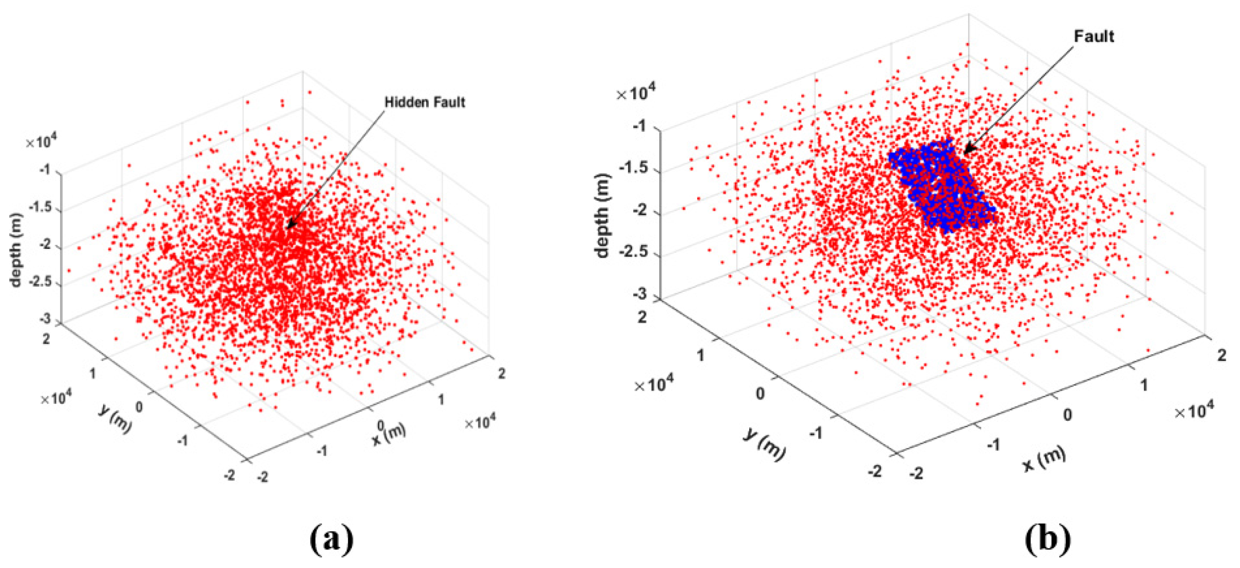
In the second case (Figure 4), is simulated the presence of a fault immersed in a normal random distribution of 5000 hypocentres (Figure 4a). We have added to the previous normal distribution a simulated fault made of 500 hypocentres with a random distribution in the x-y dimension (10 x10 km) and a normal distribution, with variance 200 m, in the z-dimension. The aligned earthquake distribution (i.e., the fault) initially on the z=0 plane, is 35 degrees rotated with respect to the y-axis and 160 degrees rotated with respect to the x-axis. The algorithm converges towards the solution which individuate the angles of the simulated fault.

Results are shown in Figure 5a and 5b, where it is shown a clear density peak which represents the presence of a well-defined fault. Figure 5b confirms the existence of a fault being there a well-defined nucleus, which individuate approximatively the simulated fault angles.

Figure 5. (a) Density diagram (normal to the fault) of events random distribution: fault detection; (b) Occurrence events as function of rotations around x and y axis (values shown in the barcode).

Figure 5. (a) Density diagram (normal to the fault) of events random distribution: fault detection; (b) Occurrence events as function of rotations around x and y axis (values shown in the barcode).

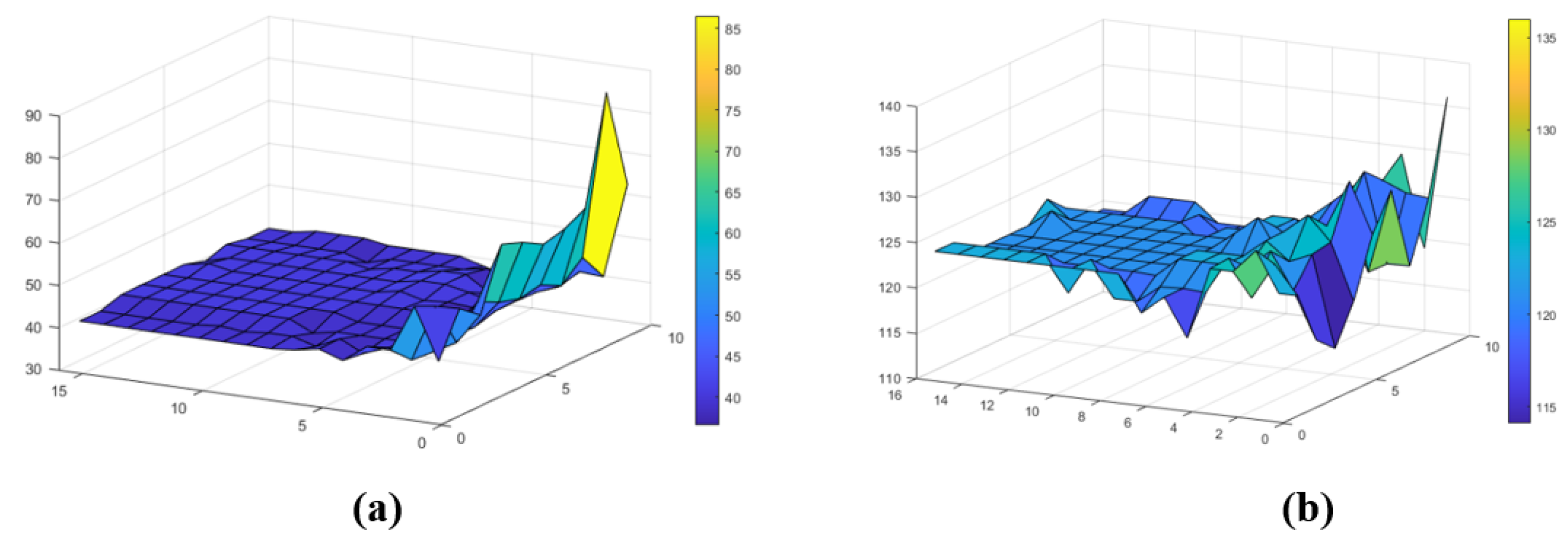
Figure 6a,b represent respectively the estimated dip and strike of the simulated fault as a function of the fault dimension and thickness. Both dip and strike are individuated where the represented functions have a stable behaviour. In particular, the estimated dip value is approximately 40 degrees and the strike value about 124 degrees, which very well matches with the imposed simulated values.

4. Application to the L’Aquila 2009 Mw6.1 Seismic Sequence

We have tested the HYDE algorithm on a very well monitored real case: the seismogenic normal fault which caused the 2009 Mw6.1 L’Aquila earthquake in Central Italy.

The L’Aquila earthquake sequence well fits the seismotectonic context of the area: seismologic, geodetic, DInSar and geological data clearly indicate that the Paganica—San Demetrio fault system (PSDFS) is the seismogenic fault of the Mw6.1, April 6 2009 main-shock [14,15,16,17,18].

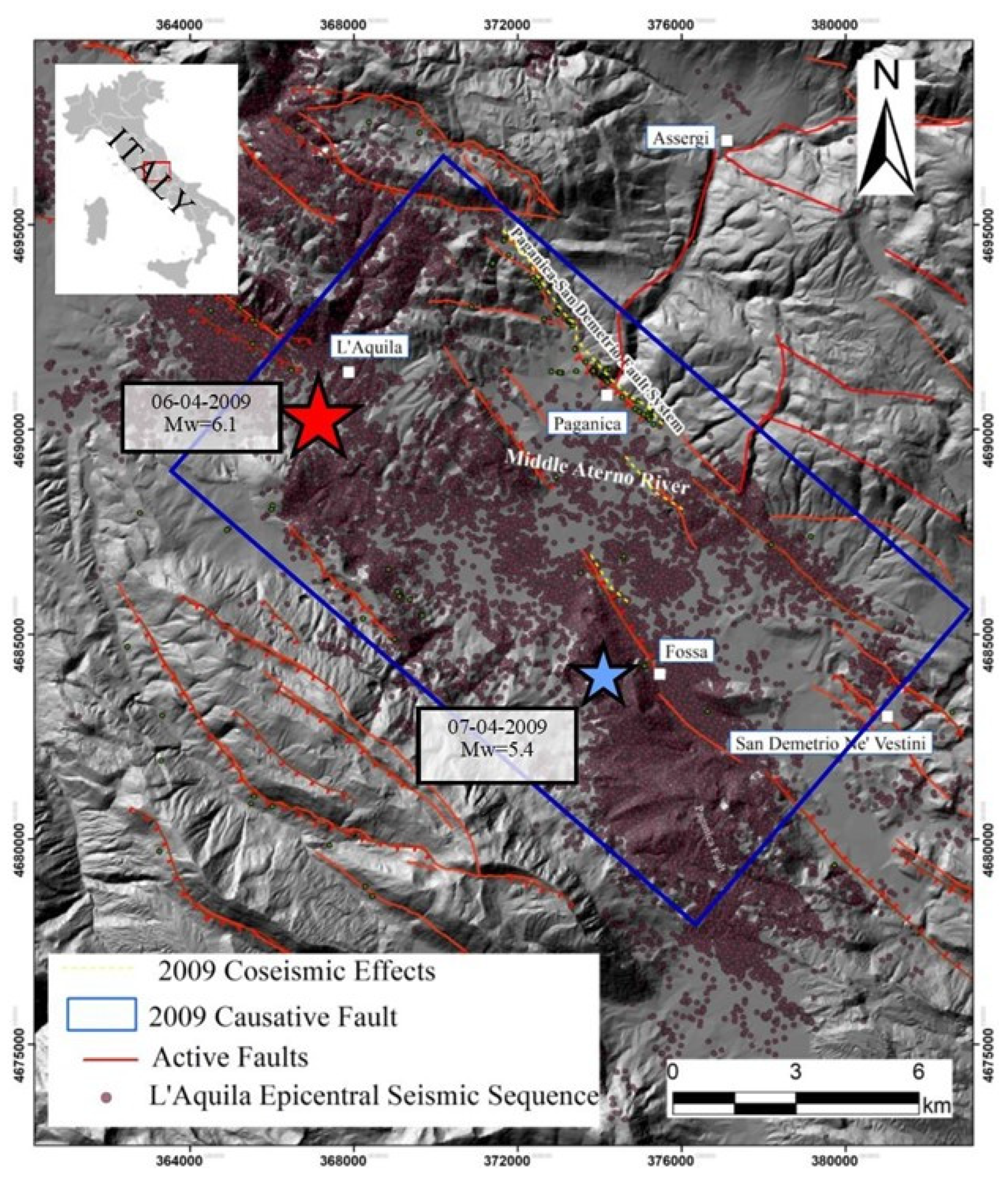
The focal mechanism indicates a fault plane with N140°direction and dipping about 45–50° to the SW [19], in agreement with the regional SW–NE extensional stress field active in the region. The seismogenic fault responsible for the 2009 l’Aquila mainshock, coincides with the surface expression of the PSDFS which bounds to the northeast the Aterno River valley (Figure 7). It shows a complex surface expression, with several synthetic and antithetic splays affecting the Quaternary basin continental deposits [20,21,22,23,24].

Before the 2009 earthquake, the geometry and activity of the PSDFS was only roughly known. It was mapped as an uncertain or buried fault [21,22,25,26].

During the 6 April main shock, this fault created a limited coseismic surface displacement observed for a total length greater than 3 km, consisting of a complex set of small scarps (up to 0.10–0.15 m high) and open cracks with a direction in agreement with the focal mechanism of the main seismic events .

Other discontinuous breaks occurred with a trend ranging from N120° to N170°, to north and south of the main alignment of ruptures. In this case, the length of the surface faulting may exceed 6 km [18,27].

Other cracks are detected along the antithetic structures of Bazzano and Monticchio-Fossa. Seismicity distribution of the 2009 L’Aquila foreshock and aftershock sequence indicates that the epicentral area has a length of 50 km along the NW-SE direction defined by a right step en-echelon fault system, with earthquakes mostly confined below 2 km [14,15,31]. This suggests that only minor slips took place on the shallower portion of the fault, in agreement with surface observations.

The 3D architecture of the Mw6.1 L’Aquila mainshock causative fault has been accurately described by [31] by using a high-quality earthquake catalogue composed of about 64,000 foreshocks and aftershocks that occurred within the first year, processed through automatic procedures. In particular, high-precision foreshock and aftershock locations delineated an about 16-18 km-long fault (the Paganica fault), showing an almost planar geometry. The aftershocks distribution around the main slipping plane varies from small (about 300 m) close to the mainshock nucleation to large (about 1.5 km) at the south-eastern termination of the fault [32]. This along-strike change in fault zone thickness has been related to the heterogenous coseismic slip distribution along the fault and to an increase in fault geometrical complexity at the south-eastern fault termination [32].

The heterogeneous 2009 coseismic rupture is well documented [33,34]. The mainshock nucleated at about 8 km depth. At first, the rupture propagated up-dip with coseismic slip located 2 km up-dip from the mainshock hypocentre; then, it continued along the strike direction to the SE portion of the fault and at shallower depths [35].

4.1. Dataset Description

Here we used a very detailed earthquake catalogue computed by [31] by processing continuous seismic data recorded at a very dense seismic network of 60 stations operating for 9 months after the M_W 6.1 mainshock. The complete catalogue is composed of about 64,000 precisely located foreshocks and aftershocks, spanning January to December 2009. It was processed by combining an accurate automatic picking procedure for P- and S-waves [36], together with cross-correlation and double-difference location methods [37] reaching a completeness magnitude (i.e., the minimum magnitude above which all the events occurring in a study area can be reliably detected and located; [38] equal to 0.7, which corresponds to a source dimension of ~50 m based on a circular crack model using a 3 MPa stress drop. Earthquake relative location errors are in the range of a few meters to tens of meters (i.e., the error ellipsoids obtained at the 95% confidence level for 200 bootstrap samples show median values of the distribution along the major/minor horizontal and vertical direction of 24, 15 and 27 m; see [39] for details. These errors are comparable to the spatial dimension of the earthquakes themselves, allowing to image the internal structure of the fault zone down to the tens of meter scale.

For this work, we use the complete large-scale catalogue, relative to the L’Aquila Mw6.1 mainshock, differently from what is shown in [35] where the authors choose earthquakes occurring within 6 km (+/- 3 km) from the L’Aquila fault plane modelled by inverting strong motion, GPS and DInSAR data. That plane is 20-km-long in the N133°E striking direction and dips 54° to SW, intersecting the mainshock hypocentre. Their resulting catalogue is made of ~19k foreshocks and aftershocks. Further details on this catalogue are described in [32], which deals with the accurate description of the L’Aquila 2009 fault zone structure and damage zone and its implication to the earthquake rupture evolution. Our large-scale and complete earthquake catalogue represents a perfect test-case to verify the ability of the HYDE algorithm to retrieve both the large and small scale complexities of the activated faults.

4.2. Application to L’Aquila dataset

We used the HYDE algorithm to define the parameters (strike, dip, length and fault zone thickness) of the Mw6.1 L’Aquila seismogenic fault, which generated the Mww6.1 mainshock and the aftershock sequence.

Following the algorithm steps, we first used the earthquake distribution to identify a set of 1000 pivot hypocentres assumed as the rotation centers of the fault plane. We made different tests, changing both the possible length of the fault plane from 4 km to 32 km (with 4 km sampling rate) and allowing the fault zone thickness to vary from 100 m to 800 m (with 100 m sampling rate), according to previous studies [32]. The initial chosen thickness of 100 m takes into account the order of the localization error, which implies a flat fault. Increasing fault thickness values will comprise non-planar faults, as it is often observed in real cases.

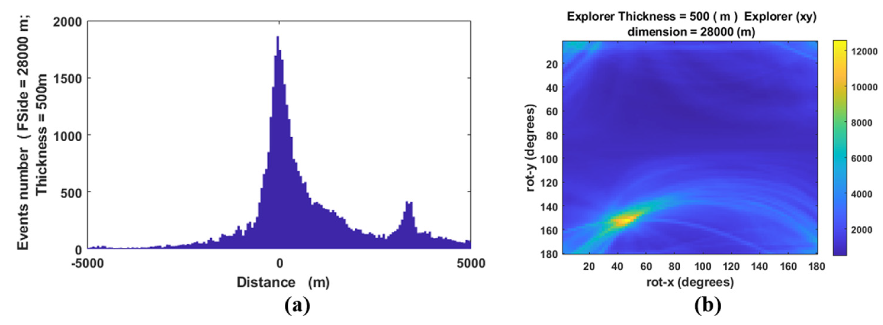
In Figure 8 are shown results for a fault zone thickness fixed at 500 m. Results (Figure 8a) show a clear density peak which represents the presence of a well-defined fault. Figure 8b confirms the existence of a fault with a well-defined nucleus which approximatively individuates the estimated dip and strike of the main L’Aquila fault.

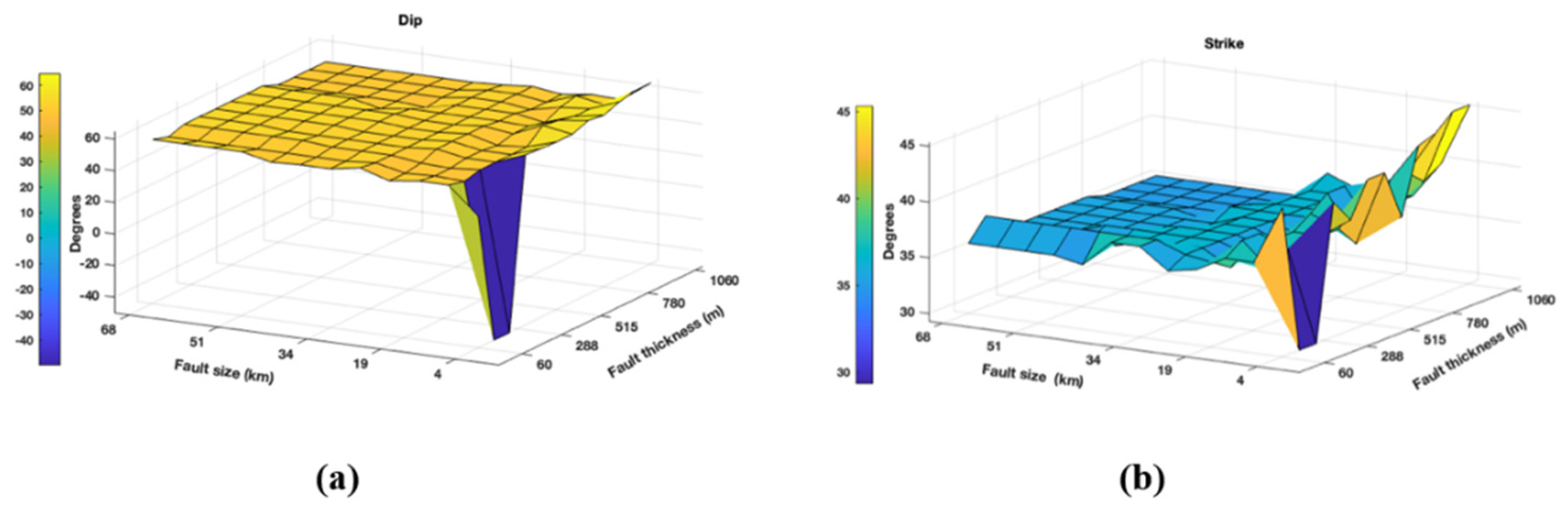
In particular, in Figure 9a,b are represented respectively the estimated dip and strike of the L’Aquila fault as a function of the fault dimension and thickness. Both fault dip and strike are individuated where the represented functions have a stable behaviour. In particular, the estimated dip value is approximately 52 degrees and the strike value about 37 degrees, which well matches the estimated values by [32,35].

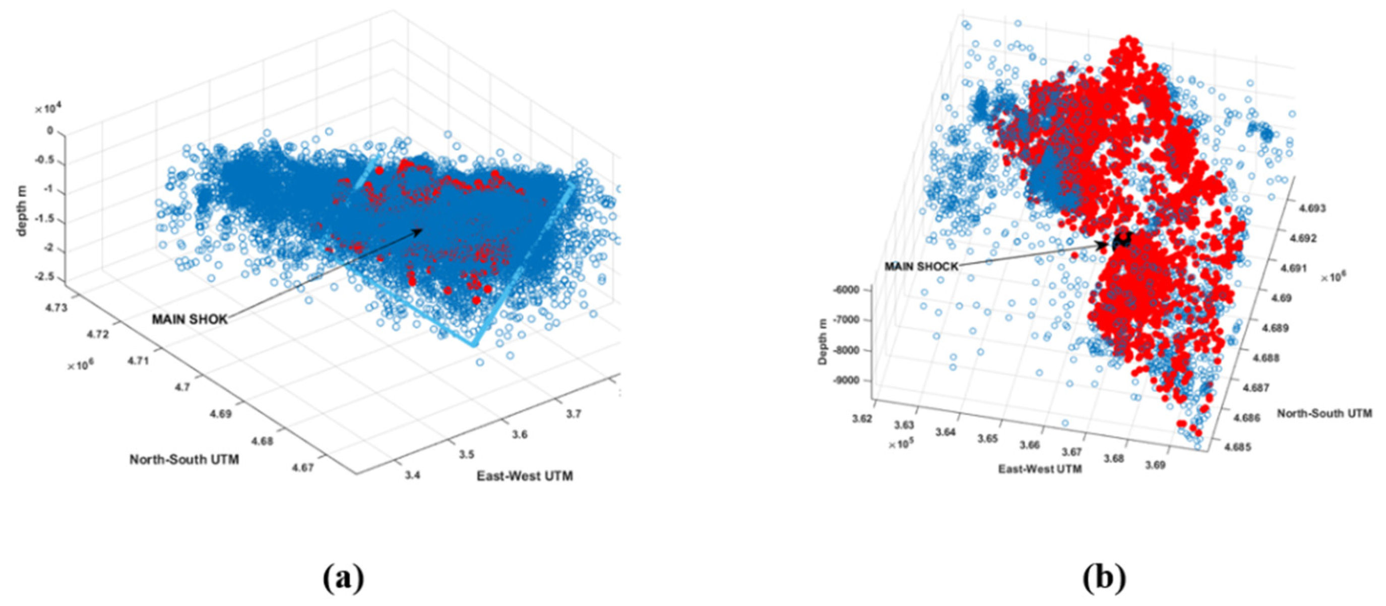
For a fault with thickness of 500 m and a length of 24000 m we obtain the solution shown in Figure 10 where it is clear that the main shock is contained into the parallelepiped which individuate the main fault plane. This is a very important result considering that the algorithm does not use constraints, as for example, ones based on the main shock location to drive the solution. This states that our algorithm is a very useful and reliable tool.

5. Conclusions

We have designed and developed an algorithm named HYDE, able to estimate the geometry (size, depth, dip and slip angles) of fault planes using hypocentre locations of the main earthquakes and the associated aftershocks, even where the seismogenic sources are fragmented. Our algorithm is particularly useful where the earthquake intensity is not so high such that the radiation pattern can be easily determined, as often happens for most of the aftershock sequences or in volcanic areas, where the percentage of earthquakes for which the radiation pattern can be defined is very low. Assuming that most of the earthquakes are clustered on fault planes, the algorithm finds the principal fault using a density driven search. It works as a Montecarlo method applied to a subspace constrained by the pivot hypocentres.

The strength of the method is based on the use of a very robust norm; it is such that when earthquakes belong to the explorer parallelepiped, they are assigned weight 1; if not, the weight is zero and this avoids the well-known problem of the outliers in the statistical analyses. Conversely, the capability to explore all the parameter space avoids the trapping of the solution into a local minimum. The algorithm easiness stands even into the use of a distance, which simply is, cause the rotation, the distance with respect to a single variable from the plane. In general, HYDE algorithm could be used even for a non-flat source geometry, for example quasi-spheric or parabolic, using the appropriate coordinate transformation.

We have tested our algorithm on a synthetic dataset and on the real case of L’Aquila 2009 seismic sequence. The obtained results for both the study cases show that Hyde is a very suitable and reliable tool being able to identify the main fault plane even in presence of many fault segments ubstructures. In particular, for the L’Aquila real case the geometry of the main fault plane, we have identified by our algorithm, is in good agreement with the independently calculated focal mechanism [32]. This validates our results paving the way to several applications where focal mechanisms are not available or not well constrained to reduce uncertainties.

Moreover, regarding the L’Aquila earthquake sequence we have performed a search using 1000 pivots to obtain stable fault parameters, but a search with only 200 pivots already gave us the same solution. This depends on the nature of the clustering of the earthquakes on the fault plane, which attracts the explorers in the right subspace reducing considerably the algorithm run time. The results of the application of our algorithm on both the synthetic and the real L’Aquila case show that HYDE is able to quickly individuate the seismogenic fault planes even for complex fault geometry. Moreover, when refined seismic catalogues are not available it is still possible to successfully use our algorithm, calibrating the thickness of the explorer parallelepiped according to the localization error magnitude. Note that the program includes the search of substructures of any dimension simply extracting data in a local subspace. Future improvement of the HYDE algorithm may include time constraints to study the hypocentre’s temporal evolution in order to explore the kinematics of the fault plains.

References

- Michell, J. Conjectures Concerning the Cause, and Observations upon the Phænomena of Earthquakes; Particularly of That Great Earthquake of the First November, 1755, Which Proved so Fatal to the City of Lisbon, and Whose Effects Were Felt as Far as Africa and More or Less throughout Almost All Europe; by the Reverend John Michell, M.A. Fellow of Queen’s College, Cambridge. Phil. Trans. R. Soc. 1759, 51, 566–634. [Google Scholar] [CrossRef]
- V. K. Borok On Estimation of the Displacement in an Earthquake Source and of Source Dimensions. Annals of Geophysics 2012, 12. [Google Scholar] [CrossRef]
- Ben-Menahem, A.; Smith, S.W.; Teng, T.-L. A Procedure for Source Studies from Spectrums of Long-Period Seismic Body Waves. Bulletin of the Seismological Society of America 1965, 55, 203–235. [Google Scholar] [CrossRef]
- Jost, M.L.; Herrmann, R.B. A Student’s Guide to and Review of Moment Tensors. Seismological Research Letters 1989, 60, 37–57. [Google Scholar] [CrossRef]
- Jones, R.H.; Stewart, R.C. A Method for Determining Significant Structures in a Cloud of Earthquakes. J. Geophys. Res. 1997, 102, 8245–8254. [Google Scholar] [CrossRef]
- Nicholson, T.; Sambridge, M.; Gudmundsson, Ó. On Entropy and Clustering in Earthquake Hypocentre Distributions. Geophys. J. Int. 2000, 142, 37–51. [Google Scholar] [CrossRef]
- Waldhauser, F.; Ellsworth, W.L. A Double-Difference Earthquake Location Algorithm: Method and Application to the Northern Hayward Fault, California. Bulletin of the Seismological Society of America 2000, 90, 1353–1368. [Google Scholar] [CrossRef]
- WAN, Y.G. , SHEN, Z.K., DIAO, G.L., WANG, F.C., HU, X.L., & SHENG, S.Z. An Algorithm of Fault Parameter Determination Using Distribution of Small Earthquakes and Parameters of Regional Stress Field and Its Application to Tangshan Earthquake Sequence. Chinese J of Geophysics 2008, 51, 569–583. [Google Scholar] [CrossRef]
- Panara, Y.; Toscani, G.; Cooke, M.L.; Seno, S.; Perotti, C. Coseismic Ground Deformation Reproduced through Numerical Modeling: A Parameter Sensitivity Analysis. Geosciences 2019, 9, 370. [Google Scholar] [CrossRef]
- Li, K.L.; Abril, C.; Gudmundsson, O.; Gudmundsson, G.B. Seismicity of the Hengill Area, SW Iceland: Details Revealed by Catalog Relocation and Collapsing. Journal of Volcanology and Geothermal Research 2019, 376, 15–26. [Google Scholar] [CrossRef]
- Zhou, Y.; Walker, R.T.; Elliott, J.R.; Parsons, B. Mapping 3D Fault Geometry in Earthquakes Using High-resolution Topography: Examples from the 2010 El Mayor-Cucapah (Mexico) and 2013 Balochistan (Pakistan) Earthquakes. Geophysical Research Letters 2016, 43, 3134–3142. [Google Scholar] [CrossRef]
- Rubinstein, R.Y.; Kroese, D.P. Simulation and the Monte Carlo Method; Wiley Series in Probability and Statistics; 1st ed.; Wiley, 2016; ISBN 978-1-118-63216-1.
- Manly, B.F.J. Randomization, Bootstrap and Monte Carlo Methods in Biology; 0, *!!! REPLACE !!!* (Eds.) ; Chapman and Hall/CRC, 2018; ISBN 978-1-315-27307-5.
- Chiarabba, C.; Amato, A.; Anselmi, M.; Baccheschi, P.; Bianchi, I.; Cattaneo, M.; Cecere, G.; Chiaraluce, L.; Ciaccio, M.G.; De Gori, P.; et al. The 2009 L’Aquila (Central Italy) M W 6.3 Earthquake: Main Shock and Aftershocks. Geophysical Research Letters 2009, 36, 2009GL039627. [Google Scholar] [CrossRef]
- Chiaraluce, L.; Valoroso, L.; Piccinini, D.; Di Stefano, R.; De Gori, P. The Anatomy of the 2009 L’Aquila Normal Fault System (Central Italy) Imaged by High Resolution Foreshock and Aftershock Locations. J. Geophys. Res. 2011, 116, B12311. [Google Scholar] [CrossRef]
- Anzidei, M.; Boschi, E.; Cannelli, V.; Devoti, R.; Esposito, A.; Galvani, A.; Melini, D.; Pietrantonio, G.; Riguzzi, F.; Sepe, V.; et al. Coseismic Deformation of the Destructive April 6, 2009 L’Aquila Earthquake (Central Italy) from GPS Data. Geophysical Research Letters 2009, 36, 2009GL039145. [Google Scholar] [CrossRef]
- Atzori, S.; Hunstad, I.; Chini, M.; Salvi, S.; Tolomei, C.; Bignami, C.; Stramondo, S.; Trasatti, E.; Antonioli, A.; Boschi, E. Finite Fault Inversion of DInSAR Coseismic Displacement of the 2009 L’Aquila Earthquake (Central Italy). Geophysical Research Letters 2009, 36, 2009GL039293. [Google Scholar] [CrossRef]
- Https://Emergeo.Ingv.It/.
- Pondrelli, S.; Salimbeni, S.; Morelli, A.; Ekström, G.; Olivieri, M.; Boschi, E. Seismic Moment Tensors of the April 2009, L’Aquila (Central Italy), Earthquake Sequence. Geophysical Journal International 2010, 180, 238–242. [Google Scholar] [CrossRef]
- Pucci, S.; Villani, F.; Civico, R.; Pantosti, D.; Del Carlo, P.; Smedile, A.; De Martini, P.M.; Pons-Branchu, E.; Gueli, A. Quaternary Geology of the Middle Aterno Valley, 2009 L’Aquila Earthquake Area (Abruzzi Apennines, Italy). Journal of Maps 2015, 11, 689–697. [Google Scholar] [CrossRef]
- Ghisetti, F.; Vezzani, L. Annales Tectonicae. Segmentation and tectonic evolution of the Abruzzi-Molise thrust belt (central Apennines, Italy).
- Boncio, P.; Lavecchia, G.; Pace, B. Defining a Model of 3D Seismogenic Sources for Seismic Hazard Assessment Applications: The Case of Central Apennines (Italy). Journal of Seismology 2004, 8, 407–425. [Google Scholar] [CrossRef]
- Vittori, E.; Di Manna, P.; Blumetti, A.M.; Comerci, V.; Guerrieri, L.; Esposito, E.; Michetti, A.M.; Porfido, S.; Piccardi, L.; Roberts, G.P.; et al. Surface Faulting of the 6 April 2009 Mw 6.3 L’Aquila Earthquake in Central Italy. Bulletin of the Seismological Society of America 2011, 101, 1507–1530. [Google Scholar] [CrossRef]
- ISPRA Geological Survey of Italy. Web Portal Http://Sgi2.Isprambiente.It/Ithacaweb/Mappatura.Aspx.
- Pace, B. Layered Seismogenic Source Model and Probabilistic Seismic-Hazard Analyses in Central Italy. Bulletin of the Seismological Society of America 2006, 96, 107–132. [Google Scholar] [CrossRef]
- Galli, P.; Giaccio, B.; Messina, P. The 2009 Central Italy Earthquake Seen through 0.5 Myr-Long Tectonic History of the L’Aquila Faults System. Quaternary Science Reviews 2010, 29, 3768–3789. [Google Scholar] [CrossRef]
- EMERGEO Working Group Evidence for Surface Rupture Associated with the Mw 6. 3 L’Aquila Earthquake Sequence of April 2009 (Central Italy). Terra Nova 2010, 22, 43–51. [Google Scholar] [CrossRef]
- Galadini, F.; Galli, P. Active Tectonics in the Central Apennines (Italy)—Input Data for Seismic Hazard Assessment. Natural Hazards 2000, 22, 225–268. [Google Scholar] [CrossRef]
- Chiaraluce, L. Unravelling the Complexity of Apenninic Extensional Fault Systems: A Review of the 2009 L’Aquila Earthquake (Central Apennines, Italy). Journal of Structural Geology 2012, 42, 2–18. [Google Scholar] [CrossRef]
- Valoroso, L.; Chiaraluce, L.; Piccinini, D.; Di Stefano, R.; Schaff, D.; Waldhauser, F. Radiography of a Normal Fault System by 64,000 High-precision Earthquake Locations: The 2009 L’Aquila (Central Italy) Case Study. JGR Solid Earth 2013, 118, 1156–1176. [Google Scholar] [CrossRef]
- Valoroso, L.; Chiaraluce, L.; Collettini, C. Earthquakes and Fault Zone Structure. Geology 2014, 42, 343–346. [Google Scholar] [CrossRef]
- Civico, R.; Sapia, V.; Di Giulio, G.; Villani, F.; Pucci, S.; Baccheschi, P.; Amoroso, S.; Cantore, L.; Di Naccio, D.; Hailemikael, S.; et al. Geometry and Evolution of a Fault-controlled Quaternary Basin by Means of TDEM and Single-station Ambient Vibration Surveys: The Example of the 2009 L’Aquila Earthquake Area, Central Italy. JGR Solid Earth 2017, 122, 2236–2259. [Google Scholar] [CrossRef]
- Cirella, A.; Piatanesi, A.; Tinti, E.; Chini, M.; Cocco, M. Complexity of the Rupture Process during the 2009 L’Aquila, Italy, Earthquake: Source Complexity of the L’Aquila Earthquake. Geophysical Journal International 2012, 190, 607–621. [Google Scholar] [CrossRef]
- Aldersons, F.; Chiaraluce, L.; Di Stefano, R.; Piccinini, D.; Valoroso, L. Automatic Detection, and P-and S-Wave Picking Algorithm: An Application to the 2009 L’Aquila (Central Italy) Earthquake Sequence. In Proceedings of the AGU Fall Meeting Abstracts; 2009; Vol. 2009; pp. U23–0045. [Google Scholar]
- Waldhauser, F.; Schaff, D.P. Large-scale Relocation of Two Decades of Northern California Seismicity Using Cross-correlation and Double-difference Methods. J. Geophys. Res. 2008, 113, 2007JB005479. [Google Scholar] [CrossRef]
- Wiemer, S. Minimum Magnitude of Completeness in Earthquake Catalogs: Examples from Alaska, the Western United States, and Japan. Bulletin of the Seismological Society of America 2000, 90, 859–869. [Google Scholar] [CrossRef]