Submitted:
07 July 2025
Posted:
08 July 2025
Read the latest preprint version here
Abstract
In physics, the two most successful theories, quantum mechanics and general relativity, appear to be incompatible with each other. Many theorists believe that the reason behind this, is that these theories treat space and time very differently, thus focus their attempts on finding a new way of modelling our universe and more specifically of modelling time [1]. In this paper we take a different approach to modelling the time dimension. We do not treat time as a fixed dimension which is experienced the same way for every phenomenon or interaction of any dimensionality. Instead, we model time to always be the plus one (+1) dimension relative to the dimensions through which a given phenomenon propagates and interacts. This means that time for one phenomenon can behave as space for a higher dimensional phenomenon whose time is a different +1 dimension. Through this dynamic modelling of time, we aim to integrate some of the mathematical tools of both quantum mechanics and general relativity such as Operators, Complex Functions (Wavefunctions), Probabilistic Behaviour, the Metric Tensor and the Einstein Energy Equation. Finally, we investigate the compatibility of our results with other theories and the possible testability of our framework.
Keywords:
space
; time
; framework
; higher dimensions
; dynamic time
; dynamic higher dimensional spacetime
; quantum mechanics
; general relativity
; special relativity
; complex numbers
; imaginary unit
; Klein Gordon equation
; gravity – induced quantum interference experiments
; mass
; emergent time
; imaginary time
1. Introduction
In the present work we will explore a new approach to modelling time in reference to space which diverges from the usual approaches. In our approach, time is not a fixed dimension which is experienced in the same way for all other dimensions, which are spatial. We model time by making it “dynamical” in nature, in the sense that it is neither fixed nor the same for different dimensional fields, their disturbances and how they interact. Our time will always be the plus one dimension to the spatial dimensions our phenomena (fields and their disturbances) interact and propagate. For a phenomenon that propagates and interacts in 3 dimensions, time is the usual 4th dimension. For a phenomenon that propagates and interacts in 4 dimensions, time will be an extra 5th dimension and for this phenomenon the 4th dimension will behave as space together with the other 3 spatial dimensions of the lower dimensional phenomena. All spatial dimensions are indistinguishable from each other and behave in the exact same way (no spatial dimension is more important or different than the other). The important parameter is not the dimension we are studying (for example the 4th or the 5th) but the number of dimensions. In such an approach, time for one phenomenon can act as space for a higher dimensional one. This may appear confusing at first and may seem prone to chaotic behaviors, but when a set of rules is applied to such a dynamic multi-dimensional spacetime framework we observe that some of the predictions of both quantum mechanics and general relativity seem to arise naturally, which in turn gives us a means to integrate mathematical tools from both theories which previously were considered incompatible with each other.
In the following sections we will try to clarify the key characteristics of a time dimension for the purpose of generalizing those characteristics according to our framework. Following that, we will focus on how a higher dimensional wave would propagate in this framework and explore how a mass term arises from such a wave, the connection with the Einstein Energy Equation, how the metric tensor seems to integrate in our framework and a potential pathway for the emergence of gravity in it. Then, we will investigate the possible ways such a wave may interact or interfere with itself and other waves and how this would appear to us, the 3 + 1 dimensional observer. Through this we will understand why observables as operators, a Hilbert space of complex functions, expectation values through integration and discontinues updates (analogous to measurements in quantum mechanics) of the 3 + 1 dimensional complex functions would be necessary for describing such waves in the 3 + 1 observers reference frame and why the results would appear probabilistic, with the observer being able only to describe correlations between them. Furthermore, we will try to derive our first most simple equation for a wave of a non-interactive scalar 4 + 1 dimensional field and compare our results with the Klein – Gordon equation and the mass term derived earlier. Lastly, we will investigate the testability of our framework by exploring possible implications it would have in our 3 + 1 dimensional frame of reference, compare some our assumptions with experimental results and examine how further experiments may validate some crucial aspects of our framework.
2. The Role and Nature of Time Across Physical Theories. Coordinate, Parameter or Emergent Dimension?
Time is one of the most fundamental and yet most mysterious concepts in physics. While it plays a crucial role in every major physical theory, serving as the evolution parameter in classical mechanics and field theory, a fixed background in quantum mechanics, and a coordinate entwined with space in relativity, physicists still do not agree on what time actually is. This section provides an overview of how time is treated across key physical theories and outlines the conceptual differences introduced by our proposed framework.
In classical physics, time is treated as an absolute, universal parameter that flows independently of physical processes. It appears as an external variable in Newton’s laws, such as in the second law F = m and is the parameter governing the dynamical evolution of a system.
In quantum mechanics, time retains its status as an external parameter and is not represented by an operator; instead, it governs the unitary evolution of the wavefunction through the Schrödinger equation
In this context:
- -
- Time governs the unitary evolution
- -
- The Hamiltonian acts on the state, while time is external.
- -
- Probabilities evolve with time and gives time-dependent spatial probability density.
- -
- 3D space is represented by operators (such as the position operator and momentum operator ) acting on the Hilbert space of states, while time remains a parameter and there’s no operator . This asymmetry is a major issue in efforts to unify Quantum Mechanics and General Relativity.
In Quantum Field Theory (QFT), the asymmetry mentioned above is resolved by treating space and time symmetrically as classical parameters that label points in spacetime, typically denoted as =(t,x) where μ=0,1,2,3. The fundamental objects in QFT are not particles, but fields, operator-valued functions defined over spacetime. Lorentz invariance in QFT ensures that time and space enter the theory on equal footing, but neither is quantized, only the fields are operator valued.
In the theory of relativity, time is treated not as an external or absolute parameter but as an integral component of the four-dimensional spacetime manifold. It is represented as the zeroth coordinate, typically written as , where c is the speed of light and t is the coordinate time. Together with the three spatial coordinates , the spacetime point is denoted with μ=0,1,2,3. The spacetime interval between two events is given by the metric:
where is the metric tensor.
In special relativity, this is usually the Minkowski metric = diag (−1,+1,+1,+1), yielding:
This invariant interval replaces the Newtonian notion of absolute time and governs the causal structure of spacetime. In general relativity, the metric becomes a dynamic field that encodes the curvature of spacetime due to the presence of mass and energy. Time thus becomes entangled with space: it curves, dilates, and behaves differently depending on the gravitational field, as described by Einstein’s field equations. In this geometric framework, time is not an independent background parameter but a coordinate with physical consequences, shaped by and contributing to the fabric of spacetime.
In higher-dimensional classical field theories, such as Kaluza–Klein theory or those theories involving the Klein–Gordon equation extended to more than four spacetime dimensions, time is typically treated as a distinguished coordinate with a unique signature in the spacetime metric. The fields are defined over a smooth manifold with coordinates = (), where μ=0,1,2,3 includes time , and a=4,5,…,D−1 denotes the additional spatial dimensions. The dynamics are governed by equations such as the higher-dimensional Klein–Gordon equation:
and is the higher-dimensional metric tensor with a Lorentzian signature to distinguish time. Time remains the parameter of evolution, and the metric signature reflects its distinction
These models are classically well-defined using real-valued fields and differential geometry. All quantities (for example: are real valued (complex numbers are not necessary to those theories in contrary to quantum mechanics which can not be described without them) and so are the Euler – Lagrange and field equations with their solutions. However, when transitioning to a quantum description in those theories, quantization is externally imposed through procedures like canonical quantization or path integrals, rather than emerging naturally from the structure of the theory. This highlights a conceptual gap: while time enters the equations through the metric as a coordinate, its role in the quantum formulation is not fundamentally derived but rather treated analogously to lower-dimensional cases.
In our approach time will be modelled as an evolution parameter that governs the dynamics of fields, but unlike traditional treatments, it is not assigned a fixed coordinate position from the outset. Instead, we propose that time emerges as the +1 dimension relative to the dimensional space through which a phenomenon (field or disturbance of this field) propagates. The reasoning behind this is as follows:
Space can be understood as a complete set of values and relations, such as geometric configurations or field distributions defined on a manifold at a given instant, while time serves as the parameter that governs the continuous evolution of these spatial configurations. In this view, the state of a physical system at any given moment corresponds to a point in a spatial configuration space, and time provides the ordering and dynamics that relate these configurations across different instants. Formally, if denotes a spatial hypersurface at time τ, then the full physical history is a trajectory through the space of configurations {} with time acting as the evolution parameter driving this trajectory. This is the reason we say that time emerges as the +1 dimension. Since space forms a complete set of values and relations, if we consider fields with different dimensionality, meaning fields that all their values and relations can be described in different amounts of dimensions, corresponding to all the necessary degrees of freedom needed to describe them, then it stands to reason that those fields would have a different time dimension. Following that reasoning if we allow these fields to interact with each other or even for one field to be a complete subset of a larger dimensional field then what functions as time for the lower-dimensional field may be embedded within the spatial structure of the higher-dimensional one. In this sense, time for one field can behave as a spatial dimension for another, and the flow of time becomes a relational and dimensional concept, not absolute or universally fixed. This allows for a dynamic, emergent notion of space and time in which dimensional roles are defined by the internal structure and propagation of the physical systems themselves.
In our approach, as will be demonstrated in the following Sections, the spacetime metric tensor is not postulated a priori, as is common in most higher-dimensional theories, but instead emerges naturally from the dynamics of field propagation, constrained by the fundamental requirements of causality and invariance. Moreover, both space and time are treated as dynamic parameters, rather than fixed, absolute constructs. Quantum mechanical behaviour arises not through imposed quantization, but through the way a lowed dimensional observer models higher dimensional interactions in their reference frame. In this context, operators emerge as the essential mathematical tools required to describe the evolution and correlations between different higher dimensional field values which evolve in a higher dimensional time and the Hilbert space formalism of quantum mechanics is not introduced artificially but appears as a natural mathematical consequence of the dynamic time behaviour. This perspective opens the possibility of a consistent and conceptually unified integration of quantum mechanics and general relativity, grounded in dimensional dynamics rather than separate foundational assumptions.
3. Characteristics of a Time Dimension and How to Generalize Them According to Our Framework.
In order to better comprehend the role that a time dimension plays in our understanding and modelling of the physical world around us and how to generalize it according to our proposed framework as the parameter that governs the continuous evolution of spatial configurations, we will start by examining the effects that a time dimension has on a periodic function.
We start with the usual 3 - dimensional wave of the form:
where = (1A), = (1B)
(A is the amplitude of the wave, ω is the angular frequency, is the wave vector, is the velocity of the wave)
In such a wave the time dimension (symbolized by t) is vital for performing two functions:
- 1)
- It propagates the wave (or more accurately the wave front) in space with speed in the direction of .
- 2)
- If we focus on a specific point in space (for example = ( ), the amplitude A of that point oscillates with time with frequency f = ω/2π as shown in Figure 1.
Every wave function corresponds to a wave equation which typically takes the form [2]:
The link between the two is the equation:
(λ is the wavelength of the wave, k = 2π / λ)
In order to model time in a dynamic way, as we mentioned in Section 1, we will focus on both of the characteristics shown above and try to generalize them together with a relation that connects the spatial dimensions with the temporal dimension, such as (3).
Regarding the first one, we are interested in propagation through space. In our framework, the time dimension of a lower dimensional phenomenon (field or disturbance of that field) acts as a spatial dimension for a higher dimensional one. This means that we must always know the dimensionality of what we are trying to model and the dimensionality of the reference frame we are interested to model it in. For example, modelling a 4 + 1 dimensional wave in a 3 + 1 dimensional frame of reference. This is one of the things that sets apart our framework from other multidimensional frameworks.
This means:
- -
- we should always define the propagation vector with the right number of components – one for every dimension of space (for example 4 components for the 4 + 1 dimensional wave)
- -
- define a relation between these components that applies for the reference frame we are modelling it in. For a lower dimensional reference frame one of these components will behave as a time dimension, so it must both be expressed in the same units as the other spatial dimensions and be connected to the other spatial dimensions through a relation that preserves causality and invariance.
- -
- define relations that connect the time dimension of the phenomenon (field or the disturbances of that field) we would like to model with the propagation vector. These relations are crucial for our framework because they are the link that connects spatial dimensions with the time dimension. Without them our framework would be prone to chaotic behaviors and results that do not correlate with our physical reality.
Focusing on the second characteristic, we turn our attention to a specific point in space. Here we should also be very careful of the dimensionality of what we are trying to model and the dimensionality of the reference frame we are interested to model it in. We must always take the same spatial dimensions as the spatial dimensions our interacting phenomenon (field or disturbances of that field) has and examine how a specific value of this space changes with respect to the time dimension of the interacting phenomenon. For example, for a 4 + 1 dimensional wave the specific point in space we would study should also have 4 components and a specific value of this 4 – dimensional point should change in relation to the 5th dimension.
This may appear very confusing since a 3 + 1 dimensional observer would have no way of measuring the 5th dimension and in that observer’ s reference frame it would seem as a specific point in space in a specific point in time (4th dimension) has many values. This is why we need relations such as the ones mentioned above that connect the temporal with the spatial dimensions so that our results remain consistent.
Finally, a crucial aspect of reality that our framework should uphold is causality and the speed of light. These should hold true for every reference frame of any dimensionality no matter the dimensionality of the phenomenon we are studying.
With all the above in mind, we will try to model a 4 + 1 dimensional wave in the reference frame of a 3 + 1 dimensional observer, with proper relations that connect the temporal with the spatial dimensions and correspond to the rules mentioned above.
4. Modelling the Propagation of 4+1 Dimensional Waves in Our Framework. Deriving a Mass Term, the Einstein Energy Relation and Integrating the Metric Tensor in our Framework.
In this Section we will focus our attempts on modelling the propagation of a 4 + 1 dimensional wave in the reference frame of a 3 + 1 dimensional observer.
As mentioned in the previous Section, we must always know the dimensionality of what we are trying to model and the dimensionality of the reference frame we are interested to model it in. This means that we should always define the propagation vector with the right number of components (4 components for the 4 + 1 dimensional wave). Also, since we are modelling in the reference frame of a 3 + 1 dimensional observer, all quantities and relations must be modelled in the observer’s time dimension and we should conserve all relationships that apply to the observer.
Furthermore, the 3 + 1 dimensional observer cannot measure the 5th dimensional component of a higher dimensional quantity or measure changes in that dimension. However, that does not mean that the observer does not experience effects of the interactions that relate to these components. Also, there are quantities that relate changes in the higher dimensional components to the lower dimensional ones (like frequency which expresses changes in time and is connected to spatial quantities through (3)). Since those quantities are vital to the lower dimensional observer for describing higher dimensional phenomena, it would make sense for the observer to model them as quantities that are intrinsic to that phenomenon and do not change or in other words are invariant quantities. An example of such a quantity may be a quantity that encapsulates the energy and momentum of a system which should remain a fundamental concept for ensuring physical laws’ consistency across all frames, analogous to invariant mass in general relativity [3].
Considering all the above, for a 4+1 dimensional wave, space is 4 dimensional (3 - dimensional time is part of our spatial dimensions now) and all space dimensions are equivalent and treated the exact same way, meaning that our new wave vector must be 4 dimensional and have the form
now has a 4 - dimensional direction, which means that the rate of transmition of that wave will also have a 4 - dimensional direction.
(Propagation is meaningless without time. How much space is covered in how much time is expressed by velocity. Since in our framework time is not a fixed dimension from now on we will refer to the velocity of every wave (or field disturbance) of any dimensionality in relation to the wave’s time dimension as rate of transmition in order to avoid confusion with what the 3 + 1 dimensional observer considers as velocity)
Also, we should have a relation analogous to (3) which connects the 4 spatial dimensions with the 5th time dimension. This relation should also preserve the speed of light limit.
Such a general relation could be the following:
The magnitude of the rate of transmition of all waves, no matter their dimensionality, is equal to the same number c, which is equal to the speed of light for the 3 - dimensional wave.
Applying such a relation would give us:
where is the wave’s angular frequency in the 5th dimension.
The thing that remains now is to express all the above quantities in the 3 + 1 dimensional observer’s time (our time dimension) together with relations that apply to that observer (relations also expressed in our time dimension and preserve invariance).
As we mentioned before, both quantities c and A express changes in the 5th dimension, so it would make sense for the 3 + 1 dimensional observer to express them as invariant quantities.
The new wave vector is a quantity that has real physical significance to the observer but depend on the observer’s reference frame. It has 4 components, 3 corresponding to the observer’s spatial dimensions and 1 corresponding to the observer’s time dimension. However, for a 4 + 1 dimensional phenomenon, the observer’s time dimension behaves as space. This means that we must express all the components of this vector with the same units and utilize the correct relations in order to express the magnitude of that vector. The solution is something that is very common in modern physics:
in the 4+1 dimensional frame of reference, would be modelled as
in the 3 + 1 dimensional reference frame.
The minus sign is utilized because since both A and c remain constant in our approach, the quantity should also remain constant. This means that any change in magnitude of any of the components would correspond to an opposite change in some other component. Since the 3 + 1 dimensional observer experiences the 4th dimension as time it would make sense to model the 4th dimension differently and ̎group̎ those changes (that should always cancel each other out) as changes in the observer’s space and changes in the observer’s time.
Alternatively, in the formalism of vector analysis all this can be expressed as:
At this point we see how the use of the metric tensor can be integrated in our framework.
Combining (4) and (5) we get:
Taking the square of (6) in order to get rid of the square root in the denominator we get
multiplying both sides with in order to get units of energy we get
For equation (7) we have used the deBroglie relation:
= /λ = and the Einstein – Planck equation: E =
which apply to all fundamental particles [4].
Comparing (7) with the Einstein energy equation:
we find that every 4-dimensional wave that obeys the rules we imposed on our framework should have a property which behaves like mass and is proportional to the wave’s angular frequency in the 5th dimension noted by the letter .
By relating the quantity with mass we conclude that:
Summarizing the above, we see that 4 + 1 dimensional waves in our framework exhibit a property which is identical to a mass term and is proportional to the wave’s angular frequency in the 5th dimension. Also, inserting (9) to the frequency-wavelength relation (4) produces the correct form of the Einstein energy equation.
All these indicate that 4 + 1 dimensional waves in our framework have mass and propagate in 3-dimensional space with velocities less than those of the speed of light. Also, the bigger their velocities in 3-dimensional space is, the less their velocity in the 4th dimensional time. This is derived from (6) which becomes
Additionally, we saw that the metric tensor arises naturally from our framework. This is important because the metric tensor is a central object in general relativity that describes the local geometry of spacetime, thus making our framework compatible with the framework of general relativity [3].
Taking all the above into account, we can go even further and try to integrate gravity into our framework.
A first approach can be made by modelling the 4 dimensional space for the 4+1 dimensional wave (or equivalently the 4 dimensional spacetime for the 3 + 1 dimensional observer) as an anisotropic medium, where the magnitude of the rate of transmition of the 4+1 dimensional wave (mentioned above) varies according to the energy distribution inside a certain region. This approach is similar to the approach taken by analogue gravity [12,13], transformation optics [14,15], and even parts of emergent gravity research, with the difference that in our framework mass and energy are not external parameters but emergent quantities and the metric tensor is not imposed but emerges naturally.
In such an approach, we could relate the 3 + 1 stress-energy tensor , which encapsulates the density and flux of energy and momentum in 3 + 1 spacetime, with a tensorial refractive index, which affects the speed of propagation.
Such an equation could take the form:
Where is the tensorial refractive index and is connected to the speed of propagation or rate of transmition by the relation:
is the direction of propagation.
Then we could use equation (6):
to relate the metric tensor with the tensorial refractive index, which is in turn connected with the stress-energy tensor , effectively linking geometry to the density and flux of energy and momentum.
It is important to note at this point that in this approach since the metric tensor is connected to the tensorial refractive index which depends only on position and the wave’s frequency in the 5th dimension (invariant mass) is unaffected by that tensorial refractive index, the emergent metric tensor is determined only by the background therefore all 4 + 1 dimensional waves propagate through the same refractive structure and see the same emergent geometry. As a result, the geodesic motion of massive wave packets is independent of their rest mass, preserving consistency with the equivalence principle of general relativity.
This of course is only an approximation that applies only to 4 + 1 dimensional waves (massive) and their energy density and flux and does not consider other waves – disturbances of other fields (for example electromagnetic waves).
Despite that, the fact that it so nicely connects to the equations of general relativity may be a strong indication that we are on the correct path.
Furthermore, because of the approach taken above, which shows that it is possible to integrate gravity in our framework and because we are not treating the metric tensor as an independent dynamic field, but as an emergent property of wave behavior and given the inherently dynamic nature of the framework (especially its dependence on fields of varying dimensionality) it may offer a basis for interpreting and potentially integrating other phenomena, such as dark matter and dark energy. However, exploring these possibilities lies well beyond the scope of this paper.
5. Describing the Behaviour of a 4 + 1 Dimensional Wave. The Emergence of the Hilbert Space Structure of Quantum Mechanics in Our Framework.
In this Section, continuing the study of the behaviour of a 4 +1 dimensional wave in our framework, we will direct our efforts toward describing how a 3 + 1 dimensional observer can model the behaviour of a quantity that changes in reference to the 5th dimension.
In order to do that and in accordance with Section 3, we turn our attention on a specific point in 4D space = (). If the 4th dimension is treated as space, then at any such point the amplitude A of the 4th dimensional wave (not to be confused with the wave’s angular frequency in the 5th dimension which we also expressed as above) will oscillate in the 5th dimension with frequency f′ = ω′/2π as shown in Figure 2.
This means that for a specific point in space and for a specific moment in time, as a 3D observer perceives it, a 4 - dimensional wave would seem to possess many values of A which cannot be known in advance since the observer doesn’t have access to the 5th dimension.
From the very first moment we try to mathematically model a dynamic spacetime, in the sense that we explained above, problems start to arise. More specifically, is it possible for a 3D observer to describe changes that happen in the same moment in time (4th dimension), like the Amplitude oscillation mentioned above?
In order to answer this question and start giving our dynamic spacetime a mathematical foundation, we once again turn to the 3 - dimensional wave of the form given in (1) and we ask a different question which may give us some insight into our problem. Can we model some aspects of the interactions and interferences of 3 dimensional waves without the need of time, only by using space?
Not surprisingly the answer is yes. If these waves all travel with the same speed () and all obey the equation: = f λ, then we can make predictions about the Amplitude of the wave on a specific point in space in correlation with its Amplitude on another point in space and also make predictions about interference patterns if we know the geometry of the sources and the relative phases of the waves [2]. This is where complex numbers come into play. For example, in a single wave if we measure the Amplitude (A1) of the wave in one point in space we can know the amplitude (A2) of another point at distance dx from the first point by multiplying it with a phase factor in the form:
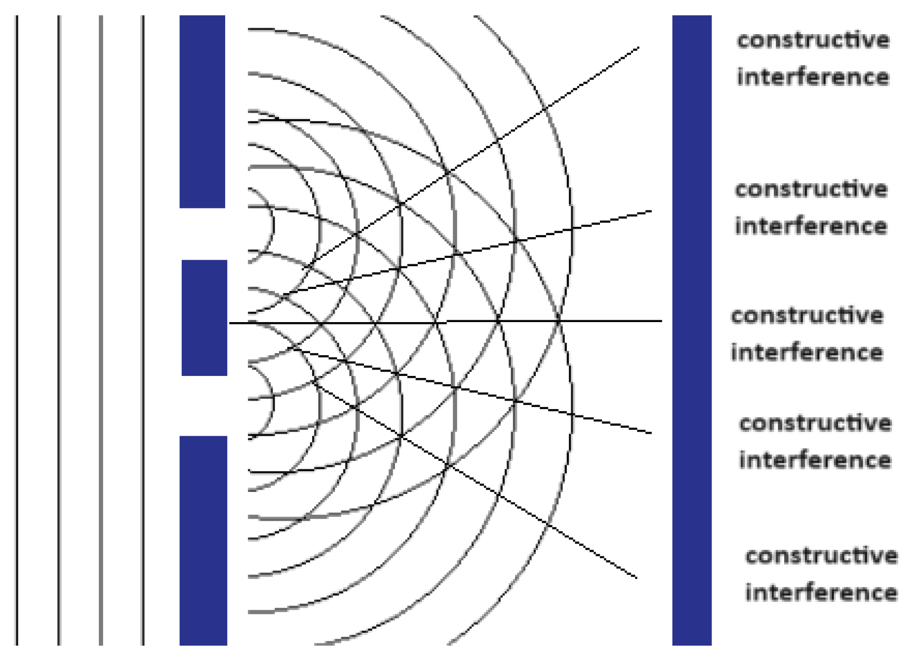
Also, in the case of the double slit experiment for light (Figure 3), we know that the Amplitude of the interference pattern for any point on the screen is analogous to + , where , the distances of the slits from the point measured on the screen and [2,9].
If there was an observer oblivious to the concept of our time (4th dimension) in any point of the screen of the double slit experiment, it would seem to him that the Amplitude of the wave can take many possible values. The only way any conclusion or correlation about the wave and its behavior can arise is with the use of complex numbers. Still some information is lost to the observer (like the exact value of the Amplitude because it oscillates with time, which the observer can’t measure or understand) but at least a great portion of the total information of the system would be accessible (for example if there is a constructive or destructive interference like in the double slit experiment for light).
Taking that into account, the observer who can’t understand and measure time would have to make use of complex functions and associate them with observables which the observer can measure and understand such as wavelength λ or energy (if the energy of a wave is proportional to its frequency which is the case for electromagnetic radiation – photons and free fundamental particles). Also, such waves can not be entirely described only by spatial functions (for example ). Using the complex plane gives us a necessary extra degree of freedom, essential for our correlations.
Complex numbers are also essential for quantum mechanics. Experiments have shown that it is impossible to predict experimental results with real-number quantum theory. Also, the use of complex numbers is apparent in the fact that we can’t derive both Planck-Einstein and deBroglie relations (E=hf and p=h/λ) in quantum mechanics without their use.
A 3D wave is oscillating both in space and in time. For two different points (x1, y1, z1, t1) and (x2, y2, z2, t2), making precise correlations about the Amplitude in different times is impossible without any information about the time separation t2-t1. Analogous to this, if we (the 3D observer) wanted to describe a 4+1 dimensional wave and model its behaviour, the only way we could achieve this would be through the use of complex numbers, using them for correlations together with quantities measurable in the 3D plane (observables) such as distance, time separation or energy. This is where the connection with quantum mechanics in our framework starts to arise, since in quantum mechanics there is also a need for operators (which are measurable quantities) in order to determine the evolution of the quantum state and its expectation values, in reference with the values this quantum state possesses in a different point in space or in time [4,5].
More specifically, if we consider a 4 + 1 dimensional wave with a constant angular frequency in the 5th dimension, meaning a constant mass in our framework (which is logical since we try to draw conclusions about the similarity of these waves and quantum mechanical particles with constant mass), the wave’s amplitude would take the form:
where x′ is the 4 dimensional space (3 + 1 dimensional spacetime for the observer) and τ is the 5th dimensional time for this wave.
Analogous to monochromatic classical waves expressed as:
where one can calculate interference and interactions without involving time, only by knowing the spatial part, which is also complex.
Additionally, translations (which refer to shifting a system in 3 dimensional space and time) would only be possible by correlating the 4 dimensional spatial function Φ0(x′) at a 4D point x′ with the 4 dimensional spatial function at another 4D point, with the spatial difference between these two points and a measurable quantity that encodes the dynamics of the system in that direction. This is analogous what happens in classical waves where we multiply with phase factors in order to correlate the Amplitude of a wave in one point with the Amplitude of that wave in another point.
Mathematically, such translations would have to be implemented through unitary operators generated by observable quantities. For a small displacement in 4D space () the function Φ0(x′) transforms as:
where would be an operator that encodes the dynamics of the system in the direction of the displacement.
Since Φ0() is not the full description of our wave solution, which evolves also in the 5th dimension, its evolution must be state-dependent and must be generated by operators not simple numbers. These operators contain the dynamical rules (e.g., frequency, mass, momentum) that determine how the wave transforms when shifted, just as the momentum operator generates phase shifts in ordinary wave mechanics.
Also, in the classical case some observed physical quantities are dependent on the square of the complex spatial part ψ(r) like intensity (the energy per unit area per unit time transported by the wave).
I(r) ∝ ψ*(r)ψ(r)
This is also the case with quantum mechanics.
All the above show that in our framework since we intend to model the behaviour of 4 + 1 dimensional waves with only spatial components (4 dimensional space for the wave), the most effective thing to do would be to use complex 4 dimensional functions. For this purpose, the natural formalism would be a Hilbert space of complex-valued functions, where:
- -
- Observable quantities, which help us make correlations, would be treated as Operators
- -
- Expectation values would encode measurable quantities we are interested in measuring and would be calculated by:
To summarize, the oscillatory wave solution of a harmonic 4 + 1 dimensional wave (which implies a particle with constant mass in our framework):
naturally suggests that the space of all such solutions forms a complex vector space. We can define a complex vector space , where Φ0(x′) ∈ and endow the space with an inner product (the superscript “2” comes from the type of integrability condition imposed on the functions in that space – real valued square-integrable functions). Observables are then modeled as linear operators acting on this space, with measurable quantities obtained via:
This formalism aligns with the Hilbert space structure of quantum mechanics, allowing us to define observables as self-adjoint operators and extract physical quantities through expectation values.
Furthermore, any interaction of such a wave which results in an irreversible exchange of energy or an irreversible change in one or more of the wave’s characteristics would have to be interpreted as a discontinuous update of the 4-dimensional complex-valued function Φ0(x′) ∈ This update can be modeled via projection operators associated with the eigenstates of a self-adjoint observable . Upon obtaining the outcome, the complex-valued function Φ0(x′) collapses to the new state’s corresponding eigenfunction and all future 5th dimensional evolution proceeds from this new state. This process parallels the standard collapse postulate of quantum mechanics referring to the quantum measurement problem.
All of the above demonstrate that the use of quantum formalism in our framework is not merely an analogy, but a mathematically necessary structure. Moreover, quantum behavior emerges naturally from the underlying dynamics, rather than being introduced through external postulates. This is also a key difference between our framework and other classical higher dimensional theories where quantum correlations are not natural outcomes and have to be imposed by turning classical fields into quantum fields, promoting classical observables into operators and then defining probabilistic behavior through a Hilbert space, that does not emerge naturally from the theory.
Finally, we will try to give the most basic form of an equation in our framework by attempting to model a pure 4 +1 dimensional wave of a Scalar Field (Φ), which does not interact with lower dimensional disturbances of itself or any other field and propagates in a harmonic way. The magnitude of its rate of transmition is taken to be equal to the magnitude of the speed of light. For this wave the 5th dimension is acting as time and the 4th dimension (our time dimension) is acting as another spatial dimension. We are interested in modelling this wave in a way that makes sense to us, the 3 + 1 dimensional observer, following the same rules we imposed on the previous Sections.
This equation would take the form:
(Second time derivative term) = (rate of transmition)2 x (second spatial derivative)
The following apply:
- -
- The wave is 4 + 1 dimensional which means that time for this wave is the 5th dimension
- -
- For this wave our time (the 4th dimension) is behaving as a spatial dimension. For this reason, our time dimension will be included in the spatial derivative terms
- -
- Since we are modelling the wave’s behaviour in the reference frame of a 3 + 1 dimensional observer, all quantities and relations must apply to that reference frame.
Taking all these into account our equation should have the form:
Considering that the wave propagates in a harmonic way in the 5th dimension and taking a sinusoidal solution Φ, the second 5th dimensional derivative term will be in the form:
(where is the wave’s angular frequency in the 5th dimension)
The second spatial derivative terms will now include 3-dimensional time (4th dimension) and we will again make use of the Minkowski metric (metric tensor for flat spacetime) because we want the results to have a physical meaning to us the 3 + 1 dimensional observer. This means that the spatial derivative terms will take the form [6]:
Combining (10), (11) and (12) we get:
which is equal to the Klein – Gordon equation if we consider that:
The same result for as the one we derived earlier!
This is very promising since the mass term we derived by alternative means in Section 4 is identical to the mass related component in the Klein – Gordon and Dirac equations [7,8]:
Also, in QFT the mass term is recognized as a term in the Lagrangian that is quadratic in the field and has the form for some ( ∝ m the mass of the particle) [7,8]. Since we can not exactly model the behaviour of 4+1 dimensional waves as we showed in this Section and need to make correlations with observables, such a term would make sense to appear in any attempt of the 3D observer to model the dynamics and possible interactions and of those waves with themselves and other lower dimensional waves.
What makes the present work fundamentally depart from other Kaluza – Klein theories, where mass is interpreted as momentum in the extra dimension is that in our approach the fifth dimension is not an extra spatial coordinate but represents a dynamical temporal dimension. This means that we do not need to rely on compactification or gauge unification and then impose quantization in order to make the equation quantum, but instead the formalism derived earlier both provide quantum behavior and compatibility with special relativity which is emergent from the framework itself.
Additionally, in other higher dimensional theories the values of the field in the fifth dimension correspond to different events in 5D spacetime and do not collapse into one 4D event unless some mechanism (e.g. compactification, brane confinement, integral over the 5th dimension) forces that [16]. This means that in those theories both the deduction of the four-dimensional Klein-Gordon equation from a five-dimensional wave equation of zero (hyper-)mass and the superposition of different values of that field in one 4D event do not work unless we use a methodology or mathematical trick external to the theory. Our framework has no use for that.
Finally, our framework provides a natural avenue for integrating different types of physical equations (including those that treat time and space asymmetrically) due to the dynamic role of the time dimension in our framework. Since time is not a fixed dimension for all phenomena (fields and their disturbances) and interactions but the +1 dimension relative to a field disturbance propagation, the mathematical form of energy dispersion may vary with dimensionality.
Take for example the case of the heat equation or diffusion in general.
It is first-order in time but second-order in space, because it models irreversible energy dispersion that depends on spatial imbalance (curvature) but has no memory or oscillatory behavior. By contrast, the wave equation is second-order in both time and space because waves involve oscillations and the acceleration (2nd time derivative) is tied to spatial curvature, reflecting the symmetric, oscillatory nature of wave propagation.
In our framework, distinctions between how space and time are treated for the same interaction may emerge naturally from the dimensional context of the interaction. For example, a higher-dimensional field could experience diffusion therefore treating lower dimensional time in a second-order, while a lower-dimensional field might also evolve in a diffusion-like, first-order way in its own time coordinate. This opens the door to a geometric reinterpretation of the Schrödinger equation (first-order in time), the Dirac equation (first-order in time and space), and even non-Hermitian dissipative systems.
Therefore, the dynamic time concept allows us to consider hybrid evolution equations (first-order in some dimensions, second-order in others) all governed by how energy propagates and disperses across interacting fields of different dimensionalities. The consideration of different fields of different dimensionalities and their interactions may also eliminate constraints between the gradients along the different coordinates (since time in one field can behave as space in another), potentially accommodating the integration of distinct symmetries and symmetry violations across different interactions, in a manner analogous to what occurs in quantum field theory (QFT). This line of thinking may allow further generalization and unification of quantum, classical, and dissipative dynamics under a common higher-dimensional geometric structure, though this is much beyond the scope of this paper.
Until now we have been focusing on wave solutions in our framework and not on system dynamics. This has been intentional because we want to focus on how both relativistic and quantum mechanical behaviour emerges from these solutions. However, the inherently dynamic structure of our model also provides a natural avenue for examining the emergence of physical laws from first principles. Let’s consider an example:
Suppose that in the context of our framework, every 4 + 1 dimensional field experiences a harmonic restoring force in the fifth dimension, aiming to restore the field to a minimum value. Such a force would take the general form:
providing that our system is conservative and we have harmonic motion in the fifth dimension.
Taking the Minkowski Metric, applying what we said in Section 4 and demanding that invariance must be conserved we derive:
f = - , where f is the projection of F onto a unit 4vector = (
If we require that energy is conserved in the 3 + 1 dimensional reference frame, which means that = 0, and the evolution of the field is governed by the spatial derivatives of energy, then the integral δx dt, in a specific direction x, which is the action for a 3 + 1 dimensional observer is:
This means that there exists a minimum non-zero variation in action corresponding to the smallest physical influence a system can undergo in this framework. As a result, the total contribution of all those 4 forces projected to the 3 + 1 dimensional reference frame from all possible directions to a certain 4 dimensional point, would be
and consist of all possible
from all possible directions, resulting in distinct (quantized) units of action.
δS = f δx δt
This postulated quantization aligns with the principles underlying both the Bohr–Sommerfeld quantization rule:
and the path integral formulation of quantum mechanics, where transition amplitudes are weighted by a phase factor:
This means that quantization may not need to be postulated externally in our framework but could emerge from the deeper structure of how higher-dimensional dynamics project into the observable 3+1-dimensional world, requiring that energy and causality are preserved under projection.
6. The Preservation of Bell’s Inequality Violation in Our Framework and How It Differs from Classical Higher Dimensional Theories.
Bell’s Theorem is a foundational result in quantum mechanics that shows that no theory of local hidden variables can reproduce all of the predictions of quantum mechanics. The Clauser-Horne-Shimony-Holt (CHSH) version of Bell’s inequality, which is commonly tested in experiments states:
If we assume the outcomes of independent binary measurement results (let’s denote them A1,A2 and B1,B2) are determined by hidden variables λ, with a probability distribution ρ(λ), then expected value (correlation) of outcomes for settings and is
Under local realism, the following must hold:
In quantum mechanics the above does not apply because quantum states like the Bell’s state = ( - ) can exist which allow S to take values greater than 2 such as 2
Classical higher dimensional theories that obey locality and do not allow faster than light information exchange, also obey Bell’s inequality S ≤ 2 because even if the hidden variable is dependent on the higher dimension and evolves in time then the possible values it can take also obey a distribution with distribution probability ρ(λ) considering that the values of the measurement settings are independent of each other and that measurements are happening in a single point in space and in time.
Despite this, our framework does not fall in the above category. That is because in our framework for a higher dimensional field the 4th dimension is behaving as space and the new 4 dimensional space evolves through the 5th dimension which now behaves as time, there are allowed correlation that are stronger the classical ones and can violate Bell’s inequality.
Take the solution Φ(x′,τ) = Φ0(x′) proposed in Section 5
If we are working only with the 4D spatial solution Φ0(x′) = K(x′) where x′ is the 4 dimensional space (3 + 1 dimensional spacetime for the observer), we can produce states with stronger correlation such as Bell’s states
Consider two orthogonal states: Ψ1(x1′) = and Ψ2(x1′) =
By forming a superposition these states we can create a mixed state Ψ(x1′, x2′) = ( Ψ1(x1′) Ψ2(x2′) + Ψ1(x2′) Ψ2(x1′) )
which also violates Bell’s inequality without the need of faster than light information exchange or the dependence of measurement settings.
Conceptually what allows stronger correlations in our framework is that for higher dimensional fields all states evolve in the higher dimension (+ 1 dimension) and the 4th dimension behaves as space. That means that the measurements of the 3 + 1 dimensional observer do not form a complete set which in turn allows for the possibility of stronger correlations without the need for faster than light information exchange.
7. The Compatibility of Our Framework with Physical Reality and Its Testability
Considering the results of the previous Sections, we conclude that in our proposed framework all higher dimensional field disturbances or interactions exhibit a property analogous (if not equivalent) to mass which produces the correct Einstein Energy Equation. Also, they propagate in 3-dimensional space with velocities lower than the speed of light and the more their 3D speed component approaches the speed of light the less their 4-dimesnional time speed component would be. This behaviour emerges directly from the invariant structure imposed on the propagation dynamics, which in turn makes the integration of the metric tensor possible.
Additionally, we demonstrated that modelling exactly the behaviour of such disturbances or interactions in our 3+1 reference frame is not possible because of our lack of information regarding the 5th dimension. Instead, we can model their behaviour by making correlations with measurable, in our 3D plane, quantities and thus have a picture about interferences, dispersions and propagations. In this context the Hilbert space structure of quantum mechanics becomes a necessity. Also, any irreversible change in a 4 + 1 dimensional field configuration (wave solutions) would result a discontinuous update in the complex-valued 4 -dimensional space wave function which is analogous to measurement updates in quantum mechanics.
Summarizing the above we conclude that all higher dimensional filed disturbances or interactions exhibit behaviour which is compatible with both quantum mechanics and special relativity. This compatibility should also apply to the interactions of these disturbances with lower dimensional fields or lower dimensional disturbances of themselves.
Although we have primarily focused on analysing the behaviour of solutions rather than full system dynamics, our model suggests that deeper aspects of physical reality may also emerge naturally from the geometric and dynamic structure of the framework. The appearance of the metric tensor from wave dynamics offers a path toward integrating general relativity and gravity. The dimensional difference of fields may eliminate constraints between the gradients along the different coordinates (since time in one field can behave as space in another), potentially accommodating the integration of distinct symmetries and symmetry violations across different interactions. A harmonic restoring force in fifth dimensional fields may result in a minimum physical influence a system can undergo possibly hinting at the quantization of action. Taken together, these results highlight the potential of our dynamic time framework not only to reconcile quantum and relativistic theories, but also to ground them in a unified higher-dimensional geometric structure that is fundamentally consistent with observable physical reality.
Despite all these, the reader may still wonder why may this framework be conceptually important and nothing more than a mathematical convenience. The key lies in its explanatory power: rather than imposing quantum or relativistic behaviour through independent axioms or quantization procedures, the framework allows these features to emerge organically from the deeper dynamic structure of our framework and the requirement that causality and invariance between reference frames be conserved. It offers a coherent interpretation of mass, the role of complex numbers, probabilistic measurement, and even spacetime curvature, all in a single framework.
As for the unintuitive behaviour of time in our framework and why such a behaviour is not obvious in our physical reality the following answer may be given. We must recognize that our perception of physical reality arises solely through interactions. All measurable quantities, observations, and physical phenomena are mediated by fields that couple to our sensory apparatus or instruments, most notably the electromagnetic field. If we interpret the electromagnetic field as fundamentally a 3+1-dimensional field (a field whose excitations - light - propagate in three spatial dimensions with time as the fourth) then our entire observational framework is inherently constrained to this dimensionality. However, if these 3+1 dimensional fields interact with higher-dimensional field disturbances, such as 4+1 dimensional waves associated with mass-bearing particles, the resulting interactions can exhibit features that are traditionally attributed to quantum mechanics as our framework suggest. Additionally, that would mean in our framework that massive particles propagate with velocities lower than that of the speed of light therefore the maximum possible velocity (that of light) would also be the speed of causality and information exchange. Furthermore, while atoms themselves are fundamentally quantum mechanical and do not adhere to strict classical 3D geometry, molecules are shaped by electromagnetic interactions (we have taken the electromagnetic field to be 3 + 1 dimensional), which depend on the relative 3D spatial configuration of atoms. Intermolecular forces, too, are governed by these electromagnetic relationships within three-dimensional space. As a result, the macroscopic structures and forces that define our physical environment emerge in a way that reinforces the appearance of a fundamentally 3-dimensional reality. All the above show that a framework like the one we are proposing would allow the reconstruction of all observable aspects of physical reality within a 3+1-dimensional reference frame, preserving the illusion that time is universally the fourth dimension, even though, at a deeper level, time itself is dynamic and context-dependent.
Finally, our framework also exhibits some other aspects that are not integrated in other theories and it is these aspects that should provide us with a means of testing it.
In Section 3 we equated the 5th dimensional frequency with a term proportional to the quantity .
Consider the well-known optical case where a 3+1 dimensional wave beam (e.g., light) is split into two paths: one beam passes through a medium that reduces its speed (depending on the refractive index), while the other travels through free space. Although the frequency remains constant, the differing optical paths introduce a phase difference between the beams, leading to interference effects upon recombination. This phase difference depends on the optical path length, which in turn is influenced by the frequency of the light due to the refractive index of the medium.
Analogously, if a 4+1 dimensional wave beam were split into two components, each traversing regions with different propagation characteristics, the resulting interference upon recombination would depend on the fifth-dimensional frequency of the wave which we equated to mass (9). This is in accordance with the gravity – induced quantum interference experiment in 1975 by R. Colella, A. Overhauser and S. A. Werner and their results published in Physical Rev. Lett. 34 (1975) 1472 [10], which say that the effects depend on the quantity . In their setup, both beams passed through regions with differing gravitational potentials, analogous to differing propagation rates in our model. These findings are also consistent with our proposed treatment of 4-dimensional space as an anisotropic medium, where the transmission characteristics of a 4+1 dimensional wave vary according to the local energy distribution.
Furthermore, in our framework, our time dimension (4th dimension) can behave as space for a higher dimensional interaction. All spatial dimensions should behave in the exact same way and be indistinguishable from each other in the higher dimensional reference frame. This implies that there should be no restriction in the direction of motion of a higher dimensional disturbance in the 4th dimension. Taking into account that we have not considered the effects of entropy and the 2nd law of thermodynamics, which may restrict this direction of motion, experimental findings that suggest results with negative time correlation should be a strong supporter of our framework. These results should not however affect causality or provide faster than light propagation of information since it would violate the rule we imposed on Section 4. The results of recent research [11] done by a team in the University of Toronto suggest that negative values taken by time such as the group delay have more physical significance than has generally been appreciated, may be one of those results in favor of our framework.
8. Summary
Through a novel way of modelling the time dimension we constructed a framework which allowed us to explore new ways of integrating quantum mechanics and general relativity by dynamically linking temporal and spatial dimensions, which are typically treated as distinct in these frameworks.
We demonstrated that under this framework higher dimensional filed disturbances or interactions exhibit properties analogous to mass and obey relationships consistent with the Einstein energy equation. This dynamic treatment of time also naturally incorporated the metric tensor, suggesting compatibility with general relativity. Furthermore, the probabilistic behaviour and need for observables in quantum mechanics, alongside the Hilbert space formalism of quantum mechanics emerged as an intrinsic feature of the framework.
The possibility of integrating some of the mathematical tools of both quantum mechanics and general relativity, in particular: Operators, Complex Functions (Wavefunctions), Probabilistic Behaviour, the Metric Tensor and the Einstein Energy Equation, offers a promising avenue for unifying quantum mechanics and general relativity, potentially solving one of the greatest problems of modern physics. Also, certain features of our framework seem to be in accordance with experimental results and we also suggested potential experimental directions to further test it.
Future research should delve into refining the mathematical foundation of this framework, investigating how interactions of higher and lower dimensional fields should be modelled, and exploring its compatibility with emerging experimental data. Finally, we believe that modelling the interaction of 4+1 dimensional and 3+1 dimensional fields together with imposing symmetries on them could be of much significance and possibly help better understand or more accurately produce some of the possible interactions and equations in QFT. These efforts may further validate and expand the scope of this dynamic higher-dimensional spacetime framework, bridging the gap between the two most successful theories of modern physics.
Author Contributions
The concept of a dynamic time dimension, as described in this paper, its core idea and the framework in which behaves are attributed to the author alone. The same is true for the for the writing of this paper and all its results.
Funding
The author declares that no funds, grants, or other financial support were received for the preparation of this manuscript.
Data Availability Statement
All data generated or analyzed during this study are included in this published article.
Notification
For any use, sharing, adaptation, distribution and reproduction in any media or format, appropriate credit must be given to the author. This applies to this paper, the concept of time behaving dynamically and being modelled as the plus one (+1) dimension relative to the dimensions through which a given phenomenon propagates and interacts, its core idea and the framework in which behaves, as described in this paper.
References
- Penrose, R. (2004). The Road to Reality: A Complete Guide to the Laws of the Universe. Jonathan Cape.
- Newton, R. G. Scattering Theory of Waves and Particles, 2nd ed., New York: McGraw-Hill, 1982.
- Misner, C. W., Thorne, K. S., & Wheeler, J. A. (1973). Gravitation. W. H. Freeman and Company.
- Griffiths, D. J. Introduction to Quantum Mechanics 2nd ed., Upper Saddle River, NJ: Pearson, 2005.
- J.J. Sakurai, J. Napolitano, Modern Quantum Mechanics, 2nd ed., Boston: Addison-Wesley, 2010.
- Gregory L. Naber, The Geometry of Minkowski Spacetime: An Introduction to the Mathematics of the Special Theory of Relativity. Springer-Verlag, 1992.
- M.Peskin and D.Schroder, An Introduction to Quantum Field Theory, Perseus Books, 1995.
- S.Coleman, Quantum Field Theory, World Scientific, 2019.
- Feynman R. P. and A. R. Hibbs. Quantum Mechanics and Path Integrals, New York: McGraw-Hill, 1965. [CrossRef]
- R. Colella, A. W. Overhauser, S. A. Werner, Observation of Gravitationally Induced Quantum Interference, Phys. Rev. Lett. 34, 1472, June 1975. [CrossRef]
- Daniela Angulo, Kyle Thompson, Vida-Michelle Nixon, Andy Jiao, Howard M. Wiseman, and Aephraim M. Steinberg1, Experimental evidence that a photon can spend a negative amount of time in an atom cloud. [CrossRef]
- Smolyaninov, I. I., & Smolyaninova, V. N. (2022). Analogue Quantum Gravity in Hyperbolic Metamaterials. Universe, 8(4), 242. [CrossRef]
- Smolyaninov, I. I. (2013). Analogue gravity in hyperbolic metamaterials. Physical Review A, 88(3), 033843.
- Sun, F., et al. (2017). Transformation Optics: From Classic Theory and Applications to its New Branches. Laser & Photonics Reviews, 11(4), 1700034. [CrossRef]
- Philbin, T. G., Kuklewicz, C., Robertson, S., Hill, S., König, F., & Leonhardt, U. (2008). Optical analogues of black-hole horizons. Philosophical Transactions of the Royal Society A: Mathematical, Physical and Engineering Sciences, 366(1877), 1611-1639. [CrossRef]
- S. M. M. Rasouli, S. Jalalzadeh, and P. V. Moniz, “Noncompactified Kaluza–Klein Gravity,” Universe 8, 431 (2022). [CrossRef]
Figure 1.
How the Amplitude of a 3-dimensional wave changes with time (Max Amplitude = 1, T = period of the wave) for a specific point in space = (.
Figure 1.
How the Amplitude of a 3-dimensional wave changes with time (Max Amplitude = 1, T = period of the wave) for a specific point in space = (.
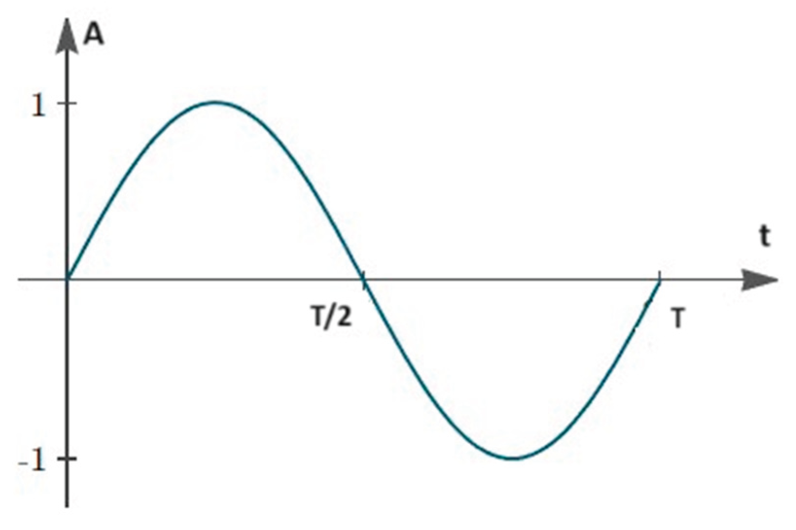
Figure 2.
How the Amplitude of a 4-dimensional wave changes in the 5th dimansion (Max Amplitude = 1, T′ = period of the wave in the 5th dimansion) for a specific point in 4D space = ().
Figure 2.
How the Amplitude of a 4-dimensional wave changes in the 5th dimansion (Max Amplitude = 1, T′ = period of the wave in the 5th dimansion) for a specific point in 4D space = ().
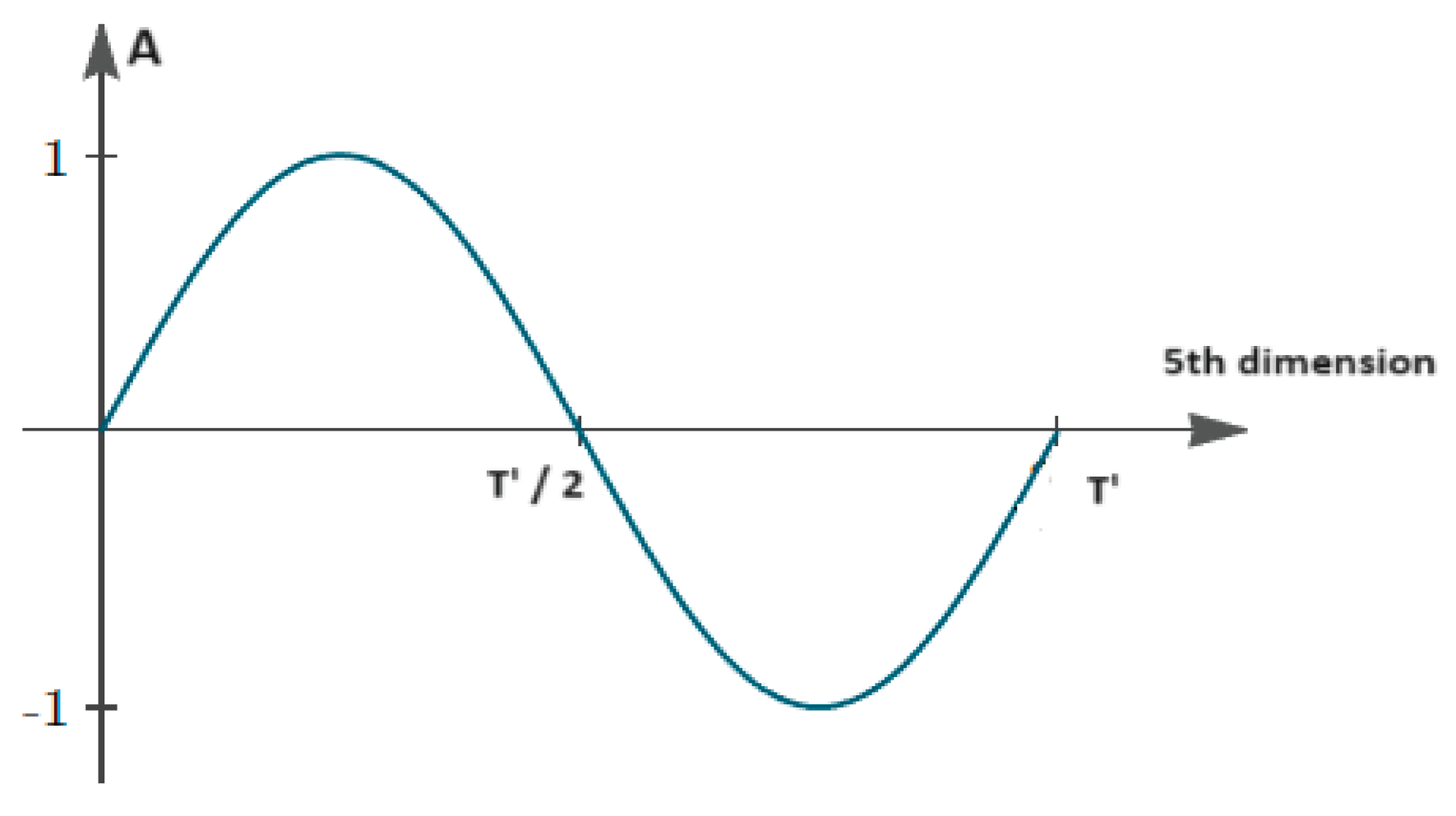
Figure 3.
The double slit experiment and how it creates constructive and destructive interferences which have to do with the geometry of the experimental setup.
Figure 3.
The double slit experiment and how it creates constructive and destructive interferences which have to do with the geometry of the experimental setup.
Disclaimer/Publisher’s Note: The statements, opinions and data contained in all publications are solely those of the individual author(s) and contributor(s) and not of MDPI and/or the editor(s). MDPI and/or the editor(s) disclaim responsibility for any injury to people or property resulting from any ideas, methods, instructions or products referred to in the content. |
© 2025 by the authors. Licensee MDPI, Basel, Switzerland. This article is an open access article distributed under the terms and conditions of the Creative Commons Attribution (CC BY) license (http://creativecommons.org/licenses/by/4.0/).
Copyright: This open access article is published under a Creative Commons CC BY 4.0 license, which permit the free download, distribution, and reuse, provided that the author and preprint are cited in any reuse.


