3D Dynamic Trajectory Planning for Autonomous Underwater Robots under the PPO-IIFDS Framework

1. Introduction

The increasing global demand for marine resource exploration and environmental protection has driven the widespread application of Autonomous Underwater Vehicles (AUV) in fields such as deep-sea exploration, seabed topographic mapping, environmental monitoring, and resource prospecting [1]. However, the complexity and dynamic nature of the marine environment—characterized by variable ocean currents, dense moving obstacles (such as ice floes or marine organisms), and irregular three-dimensional terrains—poses significant challenges to AUV navigation. Consequently, achieving efficient and reliable 3D trajectory planning for AUV in dynamic and complex environments has become a crucial research topic in ocean engineering and intelligent control.

Existing studies show that AUV trajectory planning tasks encompass three major categories of algorithms: classical graph search algorithms, heuristic algorithms, and intelligent algorithms. Each category has its own strengths and limitations and is suitable for different environmental conditions and performance requirements based on the nature of the problem and the application scenario. Specifically, classical algorithms, such as A* [2] and Dijkstra, are based on rigorous mathematical theory and are capable of finding optimal paths in known and stable static environments. These algorithms are computationally efficient and well-suited for trajectory planning problems. However, they struggle to handle dynamic obstacles, high-dimensional complex environments, and the computational burdens of large-scale problems [3]. Heuristic algorithms, such as the Artificial Potential Field (APF) method and Rapidly-Exploring Random Trees (RRT), incorporate heuristic functions or random extension strategies. These methods exhibit good real-time responsiveness and flexibility in dynamic and complex environments, enabling rapid obstacle avoidance and efficient pathfinding. However, they are prone to local optima and heavily rely on parameter tuning, which limits their ability to guarantee globally optimal solutions [4]. Intelligent algorithms, such as Deep Reinforcement Learning (DRL) [5] and Genetic Algorithms (GA), mimic biological learning mechanisms and are well-suited for handling complex and dynamically changing environments. They exhibit strong adaptability and self-learning capabilities, especially for multi-objective optimization problems. Nevertheless, the training process for intelligent algorithms requires large amounts of data and computational resources, and their results often lack stability and convergence, particularly in highly uncertain environments [6]. In practical applications, these three categories of algorithms have different applicability depending on the task characteristics and performance requirements: classical algorithms are suited for optimal pathfinding in known environments, heuristic algorithms are ideal for real-time reactions in dynamic environments, while intelligent algorithms excel at tackling highly uncertain, complex, and multi-objective dynamic tasks.

The APF method is a commonly used local planning approach, characterized by its simplicity, low computational complexity, and fast responsiveness, making it suitable for online planning. However, traditional APF methods may fail to generate feasible or optimal paths due to issues such as target inaccessibility and local optima. To address this, many researchers have analyzed and improved the APF method. One notable example is the work of Ge Shuzhi’s team at the National University of Singapore [7,8], which enhanced the repulsive potential field function to address issues such as local minima, unreachable targets, and the avoidance of moving threats. Despite these improvements, APF still lacks the concept of obstacle shapes (envelopes) and relies entirely on force field adjustments to generate paths. As a result, improper parameter tuning may cause AUVs to enter obstacles, leading to failures in obstacle avoidance. To overcome the limitations of APF, researchers proposed the stream function method based on the fundamental principles of potential fields [9,10]. This method provides advantages such as fast planning speed and smooth trajectories. However, the concept of stream functions becomes invalid when extended from two-dimensional to three-dimensional planning spaces, limiting this method to 2D trajectory planning.

To address this issue, researchers introduced a 3D trajectory planning method inspired by the "flowing water avoiding stones" principle [11], which references the macroscopic behavior of natural water flow: water flows in a straight line in the absence of obstacles, while it smoothly bypasses obstacles and continues toward its target when obstructions are present. This method integrates trajectory planning with fluid computation by introducing the concept of three-dimensional obstacle envelopes. However, traditional flow-based methods still have significant limitations: (1) analytical methods can only handle spherical obstacles; (2) due to the need for computational fluid dynamics simulations, the computational cost is excessively high, restricting these methods to offline trajectory planning.

To address the limitations of traditional flow-based methods, the Interfered Fluid Dynamical System (IFDS) algorithm was first proposed [12]. Based on analytical methods, IFDS avoids solving fluid equations with complex boundary conditions, making it suitable for handling complex terrains and various obstacle shapes. The planned routes not only retain the natural characteristics of flow-based methods but also feature simple environmental modeling and low computational cost, significantly expanding the applicability of flow-based methods. However, the streamline distribution generated by IFDS has certain limitations and is prone to local traps and stagnation points, which cannot be fundamentally resolved by auxiliary strategies alone [13]. The root cause of these issues lies in the insufficiently objective and comprehensive definition of the perturbation matrix, which limits the spatial distribution of streamlines. To address this, the Improved Interfered Fluid Dynamical System (IIFDS) algorithm was proposed [14]. By introducing a tangential matrix into the perturbation matrix, IIFDS effectively addresses these limitations. Compared to IFDS, IIFDS redefines the perturbation matrix by incorporating tangential velocity components into the perturbation flow, allowing it to point in any direction. By adjusting the repulsion response coefficients in the repulsion matrix and the tangential response coefficients and directional coefficients in the tangential matrix, IIFDS generates a variety of streamline shapes distributed throughout the planning space. These streamlines are then filtered to select paths that avoid local traps and stagnation points. However, some of these streamlines fail to meet AUV dynamics constraints or incur excessively high trajectory costs. Therefore, it is necessary to optimize the coefficients to select a trajectory that satisfies environmental and kinematic constraints while ensuring optimal performance under specific metrics or multiple objectives.

In recent years, new-generation artificial intelligence methods represented by DRL have been widely applied to the optimization and control of complex systems. These machine learning methods have several advantages [15,16,17]: (1) they do not rely on environmental models or prior knowledge, and policies can be improved solely through interaction with the environment; (2) the deep neural networks used in DRL have powerful nonlinear approximation capabilities, making them effective for optimizing high-dimensional continuous state-action spaces, which is fundamental to 3D trajectory planning in complex dynamic environments; and (3) the policies obtained through DRL require only a forward pass during inference, making them highly suitable for decision-making tasks with high real-time requirements. Based on these advantages, some researchers have explored the application of DRL in planning. For example, [18] proposed an end-to-end perception-planning-execution framework based on a two-layer deterministic policy gradient algorithm to address challenges related to training and learning in end-to-end control approaches. Similarly, [19] proposed an online collision avoidance planning algorithm based on active sonar sensors for obstacle detection. While these methods achieve good planning results, three key issues warrant further investigation:

First, DRL, as a general decision-making framework, may struggle to simultaneously ensure safety and trajectory smoothness when addressing the specific problem of AUV 3D dynamic trajectory planning. Simulation results indicate that directly using DRL to generate control inputs for trajectory planning ensures fast and safe obstacle avoidance but often produces trajectories lacking smoothness, which hinders precise tracking by low-level controllers. Combining DRL with classical heuristic methods could leverage their respective strengths in optimization speed and trajectory quality, leading to improved planning results. However, designing a hybrid framework that effectively handles complex dynamic obstacles (e.g., 3D obstacles with varying sizes and trajectories) remains an open challenge.

Second, DRL-based trajectory planning methods require agents to interact with simulated task environments and update the weights of deep neural networks based on environmental feedback. The trained deep action networks are then deployed for online planning in real-world environments. Therefore, designing simulation environments tailored to the trajectory planning methods being used is essential for improving training efficiency and ensuring the policy’s generalization in complex obstacle scenarios. Unfortunately, existing studies lack targeted research on systematic modeling methods for training environments.

Finally, high-quality trajectories must consider multiple objectives simultaneously, such as obstacle avoidance effectiveness, target reachability, trajectory smoothness, energy consumption within acceptable ranges, and adherence to AUV dynamics and kinematics constraints. Most current studies focus on single-objective optimization, which does not align with the practical requirements of AUV trajectory planning.

Contributions of This Paper:

(1) A trajectory planning framework integrating PPO and IIFDS:

This paper designs a 3D dynamic trajectory planning framework for AUVs, integrating PPO with the IIFDS. In this framework, IIFDS serves as the planning layer, dynamically adjusting flow field parameters to generate obstacle-adaptive trajectories in dynamic environments. PPO acts as the learning and decision-making layer, optimizing flow field disturbance parameters and dynamically adjusting planning strategies, enabling efficient coordination between the two algorithms in dynamic obstacle environments.

(2) Key improvements to the PPO and IIFDS algorithms:

PPO algorithm improvement: For the trajectory planning task, a multi-objective dynamic reward function is designed, incorporating obstacle avoidance, target distance, trajectory smoothness, dynamic constraints, and energy consumption. This approach effectively addresses the sparse reward problem in traditional methods, significantly improving the algorithm's convergence and the practicality of trajectory planning.

IIFDS algorithm improvement: Task-specific dynamic and kinematic constraints for AUVs are introduced into the IIFDS planning layer. This ensures that the generated trajectories not only satisfy environmental constraints but are also executable, enhancing the reliability and applicability of the planning results in real-world scenarios.

(3) Construction of a dynamic and complex obstacle environment for model training and framework validation:

A diverse dynamic obstacle environment model is developed, capable of simulating various obstacle behaviors and complex scenarios. This environment supports interactions between the agent and the environment while dynamically generating training data of varying complexity. As a result, it improves training efficiency and enhances the framework's generalization performance in practical applications. During testing, the environment validates the framework's trajectory planning performance in high-density dynamic obstacle scenarios, including the generation of collision-free trajectories, trajectory smoothness, and energy efficiency.

2. A Three-Dimensional Dynamic Trajectory Planning Framework Based on PPO and IIFDS

To simplify the analysis in this paper, the following assumptions are made:

Assumption 1: All obstacles, including both static and dynamic obstacles, are approximated as standard convex polyhedrons, such as spheres, ellipsoids, and cylindrical shapes. The mathematical representation of an obstacle’s boundary can be defined as:

${\varphi }_k\left(P\right)={\left({\displaystyle \frac{x-x_0}{a}}\right)}^{2p}+{\left({\displaystyle \frac{y-y_0}{b}}\right)}^{2q}+{\left({\displaystyle \frac{z-z_0}{c}}\right)}^{2r}-1$ (1)

where ${\varphi }_k\left(P\right)$ represents an implicit expression for the boundary of an obstacle. A value of $0$ indicates that point $P$ lies exactly on the obstacle's surface, a value less than $0$ indicates that $P$ is inside the obstacle, and a value greater than $0$ indicates that $P$ is outside the obstacle.$(x,y,z)$ are the coordinates of point$P$, while $(x_0\text{},y_0\text{},z_0\text{})$ denote the coordinates of the obstacle's center in the three-dimensional space.$a,b,c$ control the extent of the obstacle along the $x$,$y$,and $z$directions (i.e., the size of the obstacle).$p,q,r$ control the curvature of the obstacle along each direction (i.e., the exponents of the shape parameters).

Assumption 2: The information on the target location and obstacle status at the current moment is available online. This information includes, but is not limited to, position and velocity.

2.1. Introduction to the Improved Interfered Fluid Dynamical System (IIFDS)

2.1.1. Initial Flow Field Velocity Model

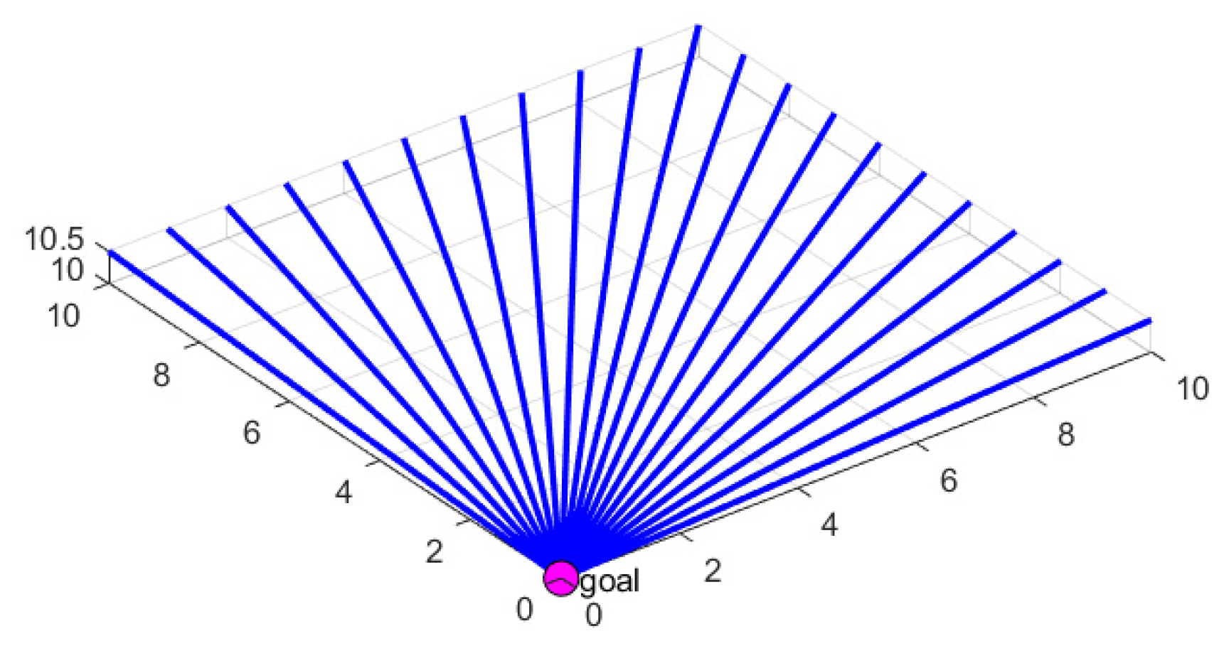
The IIFDS algorithm is based on mimicking the characteristics of natural fluid dynamics. Under conditions free from interference, the initial flow field streamlines are directed straight toward the target point. The model of the initial flow field is shown in Figure 1.

In the initial flow field, the velocity vector of the fluid passing through each position $P$, denoted as $U\left(P\right)$, can be expressed as:

$U\left(P\right)=-{\displaystyle \frac{V_0}{d\left(P,P_d\right)}}\left(P-P_d\right)$ (2)

where $U\left(P\right)$ represents the velocity vector of the initial flow field at the current position of the AUV. $V_0$ is a virtual velocity constant, used to determine the intensity of the flow field. $P=\left(x,y,z\right)$ denotes the current position of the AUV, $P_d=\left(x_d,y_d,z_d\right)$ represents the target position, and $d\left(P,P_d\right)$ denotes the Euclidean distance between the current position $P$ and the target point $P_d$, which is given by:

$d\left(P,P_d\right)=\sqrt{{(x-x_d)}^2+{(y-y_d)}^2+{(z-z_d)}^2}$ (3)

2.1.2. Obstacle Influence Modeling

When obstacles exist in the environment, their influence on the predefined initial flow field changes the fluid's velocity direction, resulting in flow field distortion. The effect of obstacles on the initial flow field is modeled using an influence matrix, defined as:

$M\left(P\right)={\displaystyle \sum }_{k=1}^K{\omega }_k\left(P\right)M_k\left(P\right)$. (4)

where $M\left(P\right)$ represents the overall disturbance matrix, ${\omega }_k\left(P\right)$ denotes the weight coefficient of the k-th obstacle, $M_k\left(P\right)$ is the disturbance matrix of the k-th obstacle, and $K$ indicates the total number of obstacles.

The weight coefficient for each obstacle is defined as:

${\omega }_k\left(P\right)=\left\{\begin{array}{c}1,K=1,\\ {\displaystyle \prod }_{i=1,i\ne k}^K{\displaystyle \frac{{\varphi }_i\left(P\right)-1}{\left({\varphi }_i\left(P\right)-1\right)+\left({\varphi }_k\left(P\right)-1\right)}},K\ne 1\end{array}\right.$(5)

where ${\varphi }_k\left(P\right)$ represents the implicit equation of the obstacle's surface, defining whether $P$ is inside, on, or outside the obstacle.

The influence matrix $M_k\left(P\right)$ of the k-th obstacle is defined based on repulsion and redirection effects as:

$M_k\left(P\right)=I-{\displaystyle \frac{n_k{n}_k^T}{\left|n_k^T{n}_k\right|\cdot T^{\frac{1}{{\rho }_k}}}}+{\displaystyle \frac{t_k{n}_k^T}{\left|t_k\right|\cdot \left|n_k\right|\cdot T^{\frac{1}{{\sigma }_k}}}}$ (6)

where $I$denotes the 3×3 identity matrix, also referred to as the attraction matrix, which functions similarly to the attractive force in the artificial potential field method. $n_k$ represents the normal vector of the obstacle's surface, $t_k$ represents the tangential vector, and ${\rho }_k$ is the repulsion coefficient that controls the intensity of the obstacle's repulsive effect. A larger ${\rho }_k$ value enables the disturbed fluid to avoid obstacles in the environment earlier. ${\sigma }_k$ denotes the tangential response coefficient, which regulates the intensity of tangential fluid flow. $T$ represents the distance from the obstacle's center to the current position, normalized by the obstacle's radius.

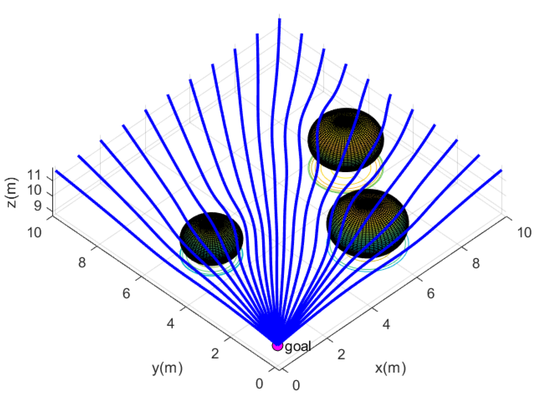
In a three-dimensional environment with obstacles, the presence of obstacles causes deviations in the original flow field paths, resulting in a disturbed flow field. This disturbed flow field is capable of avoiding obstacles while converging toward the target point. The disturbed flow field model is illustrated in Figure 2.

2.1.3. Tangential Vector Modeling

In the practical application of the IIFDS algorithm, the flow lines generated for obstacle avoidance are often restricted to a single plane, which may result in trajectories becoming trapped in local minima or stagnating at certain points. To address this issue, the IIFDS algorithm introduces the concept of a tangential matrix, allowing flow lines to move in arbitrary directions around obstacles rather than being confined to a single plane. When approaching stagnation points, the IIFDS algorithm enhances the tangential matrix to provide tangential momentum along the obstacle surface, effectively preventing the AUV from lingering at stagnation points.

On the tangent plane defined by the normal vector $n_k$, any tangential vector $t_k$​ is generated as follows:

$t_k=R_k{t}_k^{\text{'}}$ (7)

where $t_k^{\text{'}}$represents the tangential vector in the local tangential coordinate system, determined based on the tangential angle $\theta$. $R_k$ denotes the rotation matrix that transforms the local tangential basis vectors into the global coordinate system, defined as:

$R_k=\left[\begin{array}{ccc}\cos \left(\theta \right)& -\sin \left(\theta \right)& 0\\ \sin \left(\theta \right)& \cos \left(\theta \right)& 0\\ 0& 0& 1\end{array}\right]$ (8)

In this context, $\theta$ controls the rotational angle of the tangential direction, determining the specific direction for bypassing the obstacle.

2.1.4. Influence of Dynamic Obstacles

The velocity of dynamic obstacles affects the flow field through the following equation:

$v_{obs}=e^{-{\displaystyle \frac{T}{\lambda }}}\cdot V_{obs}$ (9)

where $v_{obs}$ represents the velocity influence of the dynamic obstacle at the current position. $T$ denotes the normalized distance between the current point and the obstacle. $\lambda$ is the attenuation factor, which controls the influence range of the obstacle's velocity on the flow field. $V_{obs}$ represents the velocity vector of the dynamic obstacle.

2.1.5. Comprehensive Velocity Calculation

The comprehensive velocity of the AUV is calculated using the following equation:

$\overline{U}\left(P\right)=M\left(P\right)\cdot U\left(P\right)-v_{obs}$ (10)

2.1.6. Trajectory Update

The next trajectory point is determined by integrating the velocity $\overline{U}\left(P\right)$ , according to the following equation:

${\left\{P\right\}}_{i+1}={\left\{P\right\}}_i+\overline{U}\left(P\right)\mathsf{\Delta }t$ (11)

where $\Delta t$ is the time step.

2.1.7. Heading and Pitch Angle Constraints

From the above derivation, it can be seen that traditional IIFDS does not explicitly consider the motion model and constraints of the AUV during trajectory planning. In 3D dynamic trajectory planning for AUVs, to ensure that the generated trajectory satisfies both the optimization objectives of flow-field perturbation and the motion capability constraints of the AUV itself, we introduce dynamics and kinematics constraints. These constraints primarily act on the updates of the heading angle and pitch angle, and by adjusting the next position, they ensure the physical feasibility of the trajectory.

Based on the current position of the AUV, $P_i=\left(x_i,y_i,z_i\right)$, the position at the previous time step, $P_{i-1}=\left(x_{i-1},y_{i-1},z_{i-1}\right)$, and the next position predicted by the flow field, $P_{i+1}=\left(x_{i+1},y_{i+1},z_{i+1}\right)$, the heading angle and its variation are calculated as follows:

$\mathsf{\Delta }\psi ={\psi }_{i+1}-{\psi }_i$ (12)

where ${\psi }_i$denotes the heading angle from $P_{i-1}$ to $P_i$, and ${\psi }_{i+1}$ represents the heading angle from $P_i$ to $P_{i+1}$.

If $\left|\Delta \psi \right|>{\psi }_{\max }$, the heading angle is corrected as follows:

${\psi }_{re}={\psi }_i+\mathrm{sign}\left(\mathsf{\Delta }\psi \right)\cdot {\psi }_{max}$ (13)

The correction logic for the pitch angle is analogous to that of the heading angle and is not repeated here. After completing the corrections for the heading and pitch angles, the previously planned position for the next time step is updated accordingly. The corrected position is given by:

$\begin{array}{c}{\tilde{P}}_{i+1}=P_i+\Delta s\cdot \left[\begin{array}{c}\cos \left({\gamma }_{re}\right)\cdot \cos \left({\psi }_{re}\right)\\ \cos \left({\gamma }_{re}\right)\cdot \sin \left({\psi }_{re}\right)\\ \sin \left({\gamma }_{re}\right)\end{array}\right]\end{array}$ (14)

where ${\stackrel{\sim }{P}}_{i+1}=\left({\stackrel{\sim }{x}}_{i+1},{\stackrel{\sim }{y}}_{i+1},{\stackrel{\sim }{z}}_{i+1}\right)$ represents the next position of the AUV after incorporating the dynamics and kinematics constraints, and ${\gamma }_{re}$ denotes the corrected pitch angle.

2.2. Introduction to the Improved PPO Algorithm

From Equation (6), it can be seen that the influence matrix $M_k\left(P\right)$ is not only related to the position of the AUV and the implicit equation of the obstacle's surface but also to the repulsion coefficient ${\rho }_k$,tangential response coefficient ${\sigma }_k$, and directional coefficient ${\theta }_k$ of each obstacle. If these three parameters are fixed, the resulting trajectory may fail to meet the specific requirements of certain scenarios or obstacles, leading to suboptimal trajectory planning.

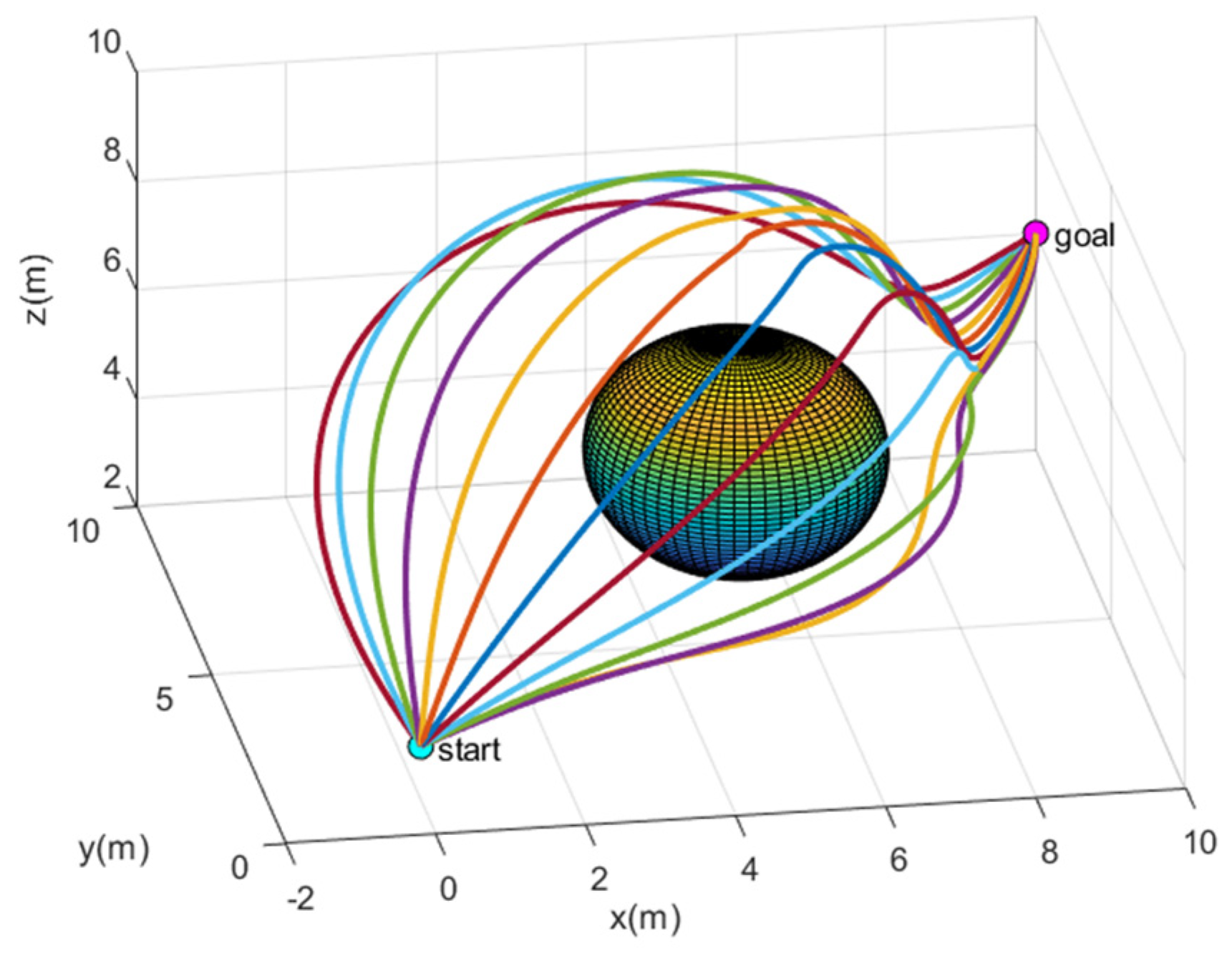
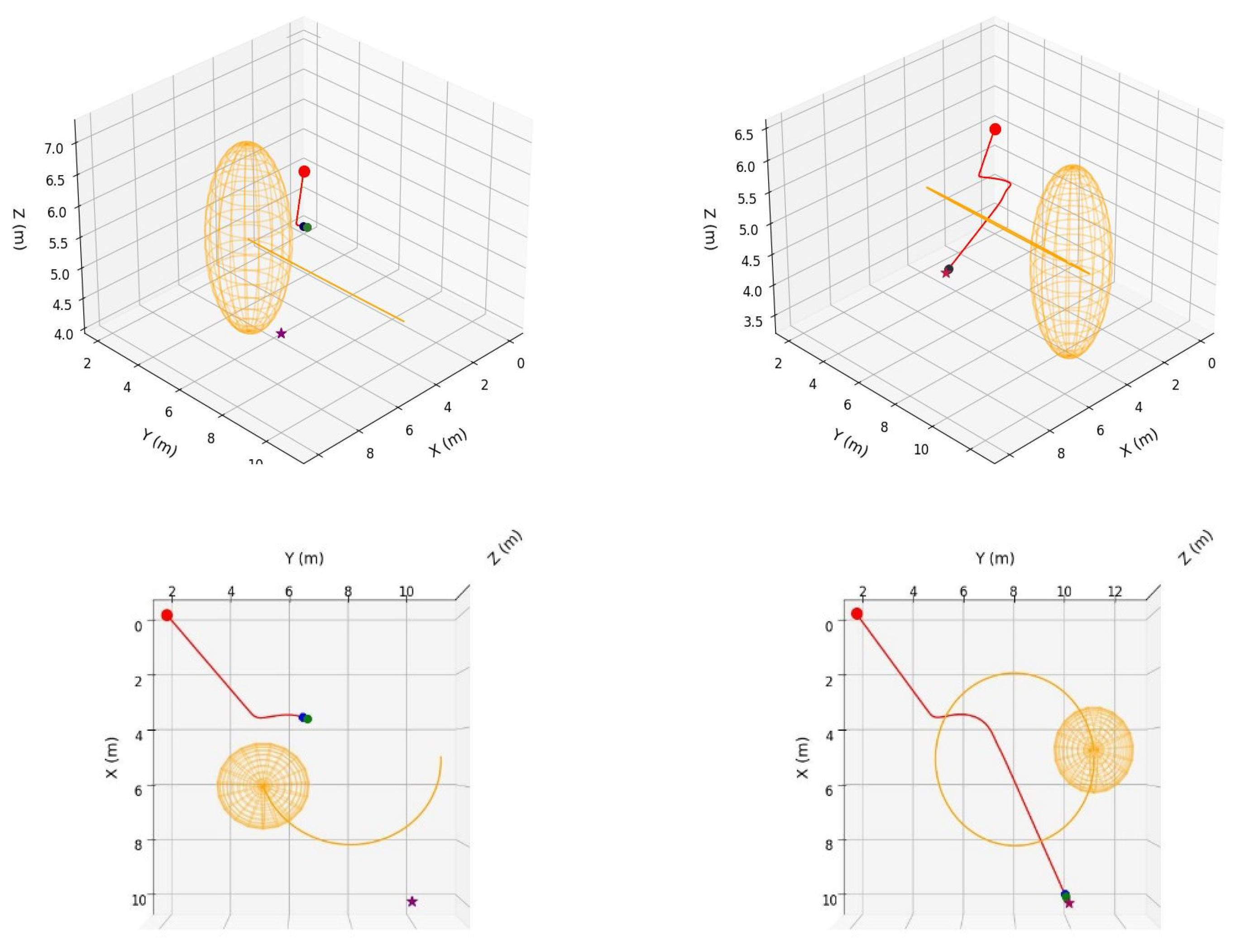
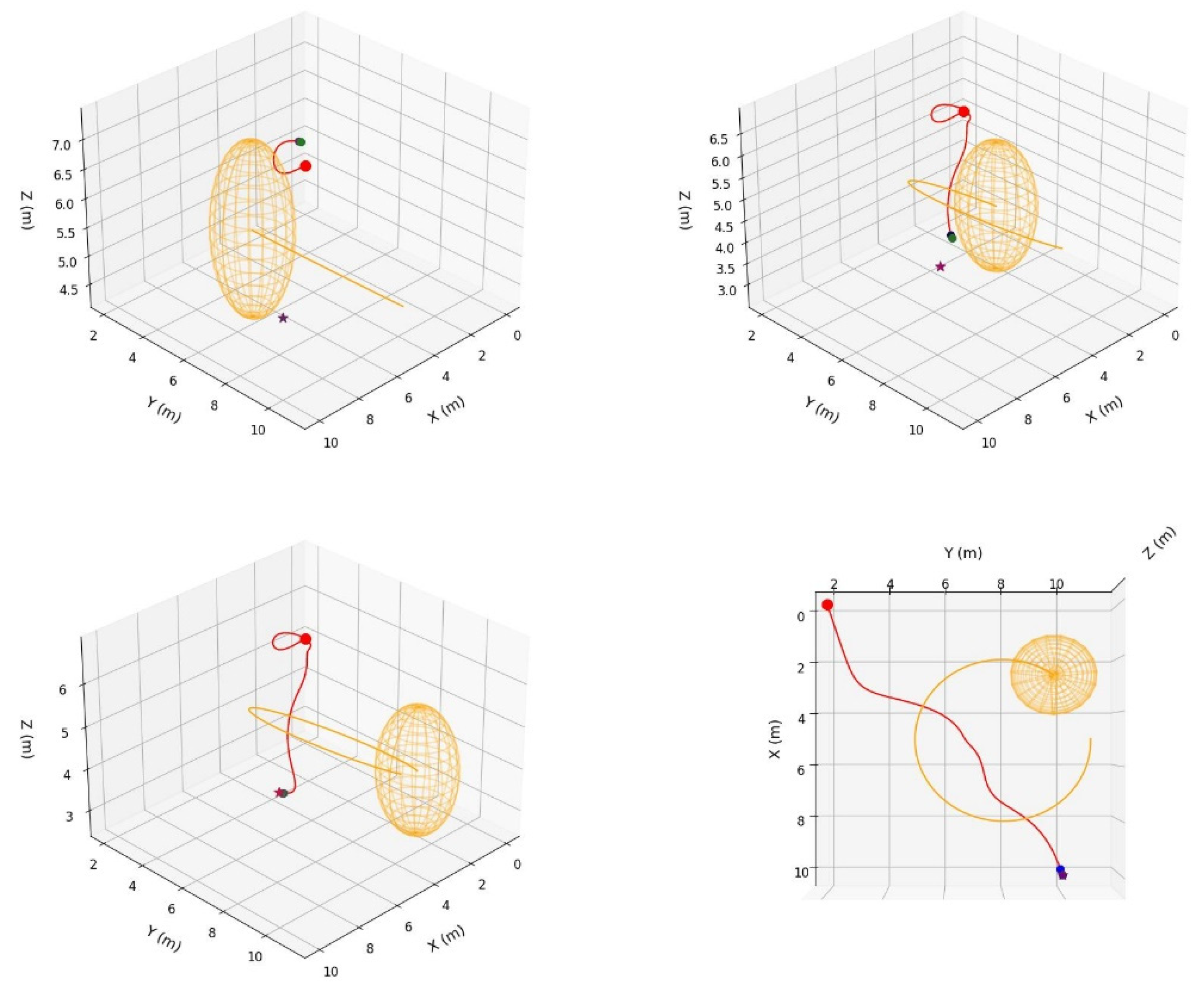
As shown in Figure 3, the plotted trajectories represent different parameter combinations. The orange trajectory in the bottom-right corner corresponds to $\rho =0.5$, $\sigma =0.5$, and $\theta =0$,From the bottom-left to the top-left corner, the coefficients increment by 0.2 for each trajectory. Different parameter combinations determine the shape and direction of the trajectories. In previous research [20], receding horizon control (RHC) has been used to optimize these parameters online. However, the serial nature of RHC's solution mechanism is not well-suited to the robustness and real-time requirements of complex dynamic obstacle environments.

PPO is a policy-based deep reinforcement learning algorithm and an off-policy algorithm. With its advantages of high stability and strong real-time performance in complex dynamic environments, we choose the PPO algorithm to optimize the three parameters of the IIFDS algorithm: the repulsion coefficient ${\rho }_k$, the tangential coefficient ${\sigma }_k$​, and the directional coefficient ${\theta }_k$​. The PPO algorithm comprises five core components: environment, agent, state, reward function, and action. The following sections will provide detailed explanations of these five components.

In the 3D dynamic trajectory planning task, the environment is a three-dimensional space that contains multiple dynamic spherical obstacles with varying radii and trajectories. In this environment, it is possible to observe the instantaneous velocities of the dynamic obstacles at any given moment, the distance between the AUV and the surface of the obstacles, as well as the relative position of the AUV to the target point. This dynamic environment simulates various complex scenarios that the AUV might encounter during real-world navigation, providing a realistic basis for testing and validating the algorithm.

In the 3D dynamic trajectory planning task, the AUV is considered as the agent.

The state space represents the collection of environmental information perceived by the agent. It comprises three vectors: the vector pointing to the target point, the vector pointing to the surface of the nearest obstacle, and the velocity vector of the nearest obstacle.

In traditional deep reinforcement learning methods, the reward function in the PPO algorithm often suffers from the issue of sparse rewards, which makes the learning process less adaptive to specific tasks. This issue is particularly pronounced in the 3D dynamic trajectory planning task for AUVs, where traditional reward designs fail to effectively guide the AUV in performing fine-grained action control. To address this, the paper introduces an improved reward function aimed at providing more precise guidance for the dynamic trajectory planning of the AUV. This reward function comprises five main components: obstacle avoidance reward, target distance reward, trajectory smoothness reward, dynamics constraint reward, and energy consumption reward.

(1) Obstacle Avoidance Reward

The obstacle avoidance reward encourages the AUV to maintain a safe distance from obstacles while considering the velocity of the obstacles. The reward is calculated as follows:

$R_{\mathrm{avoid}}=\left\{\begin{array}{c}{d}_{\mathrm{factor}}\left({\displaystyle \frac{d_{\mathrm{toobs}}-R_{\mathrm{obs}}}{R_{\mathrm{obs}}}}-1\right),if d_{\mathrm{toobs}}\le R_{\mathrm{obs}}\\ d_{\mathrm{factor}}\left({\displaystyle \frac{d_{\mathrm{toobs}}-R_{\mathrm{th}}}{R_{\mathrm{th}}}}-0.3\right),if R_{\mathrm{obs}}<d_{\mathrm{toobs}}\le R_{\mathrm{th}}\end{array}\right.$ (15)

where, $d_{factor}=1+0.5*\left|{\overrightarrow{v}}_{obs}\right|$ represents the dynamic influence factor of the obstacle’s velocity on the reward. Faster obstacle velocities increase the dynamic impact factor, which amplifies the reward’s sensitivity to obstacle avoidance.$d_{toobs}$ is the distance between the AUV and the center of the obstacle.$R_{obs}$​ is the radius of the obstacle.$R_{th}$ is the threshold radius of the obstacle’s influence zone.${\overrightarrow{v}}_{obs}$​ is the velocity vector of the obstacle.

(2) Target Distance Reward

The target distance reward encourages the AUV to move closer to the target point, with the reward increasing as it approaches the target. The reward is calculated as follows:

$R_{\mathrm{goal}}=-{\displaystyle \frac{\log \left(d_{\mathrm{togoal}}+ϵ\right)}{\log \left(d_{\mathrm{total}}+ϵ\right)}}$ (16)

where,$d_{togoal}$​ represents the distance between the current position of the AUV and the target point.$d_{total}$ represents the total distance from the starting point to the target point.

$ϵ$ is a small positive constant added to prevent logarithmic computation errors.

If the AUV is very close to the target (less than a specified threshold value), an additional bonus reward is given:

$\mathrm{if}{d}_{\mathrm{togoal}}\le \mathrm{threshold},R_{\mathrm{goal}}+=5$ (17)

(3) Trajectory Smoothness Reward

The trajectory smoothness reward is designed to encourage the AUV to move along a smooth trajectory, avoiding abrupt changes in direction, velocity, or acceleration. The reward is defined as follows:

$R_{\mathrm{smooth}}=-{\displaystyle \frac{\left|\varphi \right|}{2\pi }}\cdot 0.5-{\lambda }_1\cdot \mathsf{\Delta }v-{\lambda }_2\cdot \left|\overrightarrow{a}\right|$ (18)

where, $\varphi$ represents the angle between the current motion direction of the AUV and the direction toward the target. $\Delta v$ denotes the change in velocity between the current and previous time steps. $\overrightarrow{a}$ represents the current acceleration of the AUV.${\lambda }_1$and ${\lambda }_2$​ are weighting factors penalizing changes in velocity and acceleration, respectively.

(4) Kinematic Constraint Reward

The kinematic constraint reward ensures that the AUV's motion adheres to kinematic limits, avoiding excessive heading angles, pitch angles, and over-speeding behaviors. The reward is defined as:

$R_{\mathrm{kinematic}}=-\left({\displaystyle \frac{\left|x_1-{\psi }_{\mathrm{re}}\right|}{{\psi }_{\max }}}+{\displaystyle \frac{\left|z_1-{\gamma }_{\mathrm{re}}\right|}{{\gamma }_{\max }}}\right)-{\lambda }_3\cdot \left(\left|\overrightarrow{v}\right|-v_{\max }\right)-{\lambda }_4\cdot \left(\left|\overrightarrow{a}\right|-a_{\max }\right)$ (19)

where, $x_1,z_1$​ represent the AUV's current heading and pitch angles. ${\psi }_{\mathrm{re}}$,${\gamma }_{\mathrm{re}}$ represent the corrected heading and pitch angles. ${\psi }_{\max }$,${\gamma }_{\max }$ denote the maximum allowable variations in heading and pitch angles. $\left|\overrightarrow{v}\right|$ represents the current speed of the AUV, and $\left|\overrightarrow{a}\right|$ represents the current acceleration of the AUV. $v_{\max }$,$a_{\max }$ denote the maximum allowable speed and acceleration of the AUV. ${\lambda }_3$and ${\lambda }_4$​ are weighting factors penalizing excessive speed and acceleration, respectively.

(5) Energy Consumption Reward

This reward penalizes energy-inefficient behaviors and encourages the AUV to adopt energy-saving motion strategies. It is defined as:

$R_{\mathrm{energy}}=-{\lambda }_5\cdot |\overrightarrow{v}{|}^2$ (20)

where, $\left|\overrightarrow{v}\right|$ represents the current speed of the AUV. ${\lambda }_5$ is the weighting factor for the energy consumption penalty.

(6) Total Reward Function

By combining all the individual reward components, the total reward function is obtained, which comprehensively guides the AUV to accomplish its tasks while ensuring stable, safe, and efficient motion. The total reward is expressed as:

$R_{\mathrm{total}}=R_{\mathrm{avoid}}+R_{\mathrm{goal}}+R_{\mathrm{smooth}}+R_{\mathrm{kinematic}}+R_{\mathrm{energy}}$ (21)

The trajectories generated by the IIFDS algorithm are determined by three parameters within the algorithm: the repulsion coefficient ${\rho }_k$​, the tangential coefficient ${\sigma }_k$​, and the directional coefficient ${\theta }_k$​. Therefore, we select these three parameters as the action outputs of the improved PPO algorithm.

2.3. Optimization of IIFDS Parameters Using the Improved PPO

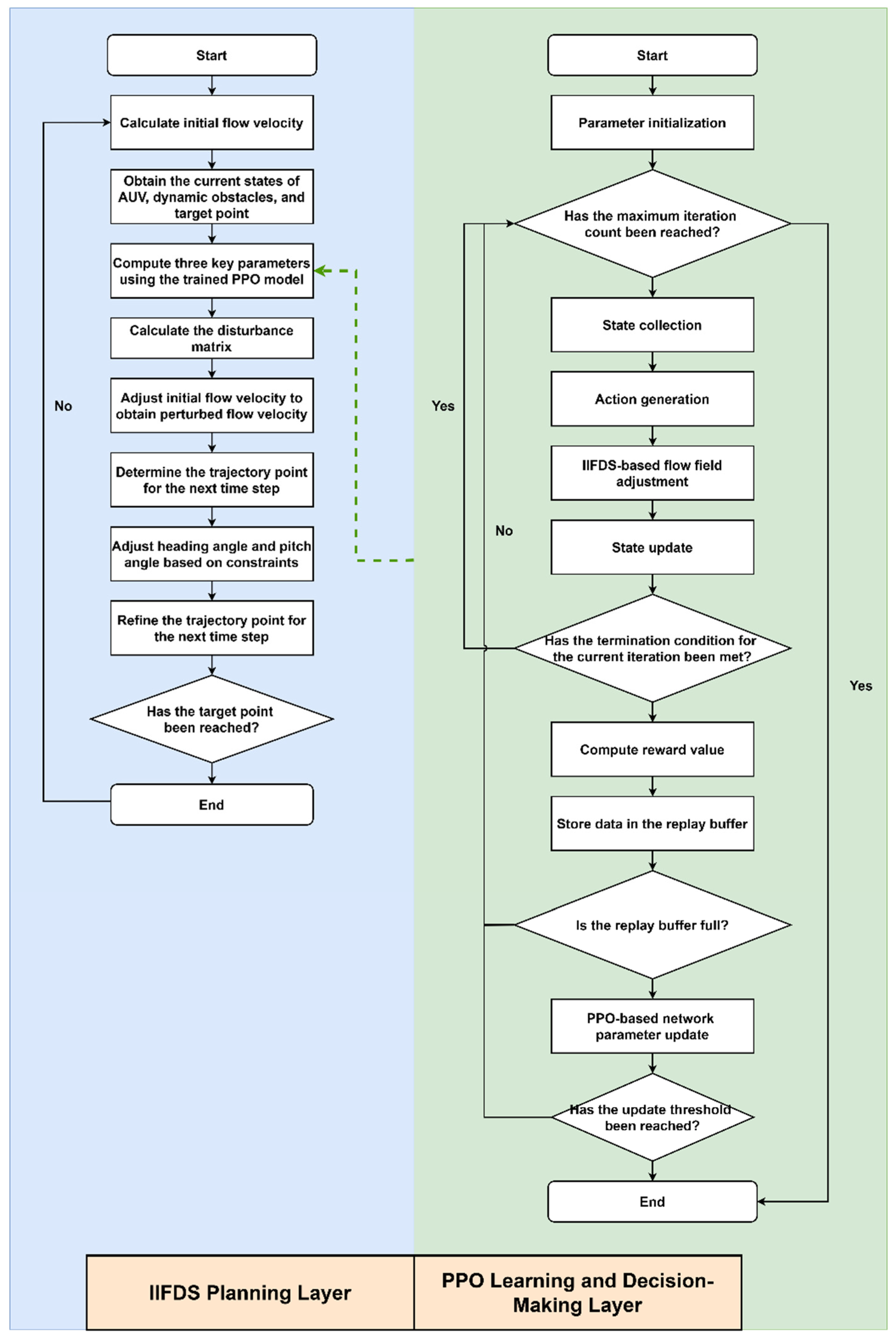
To enable trajectory planning for AUVs in complex dynamic three-dimensional environments, this paper proposes a trajectory planning framework based on the integration of PPO and IIFDS. In this framework, IIFDS serves as the planning layer, adjusting the flow field parameters dynamically to generate trajectories that adapt to moving obstacles. PPO acts as the learning and decision-making layer, optimizing the IIFDS flow field parameters, including the repulsion coefficient ${\rho }_k$ ​, the tangential coefficient ${\sigma }_k$​, and the directional coefficient ${\theta }_k$​. The detailed process of the integrated algorithm is shown in the flowchart in Figure 4.

Initialization involves setting the IIFDS flow field parameters, constructing the AUV dynamics model and dynamic obstacle environment, and defining the start and target points. Simultaneously, the Actor-Critic network of the PPO algorithm is initialized, along with the replay buffer (size 4096). Multi-objective reward functions and related hyperparameters (discount factor, PPO clipping range, learning rate, etc.) are also configured.

Subsequently, the training loop is entered, which primarily includes the main loop and the PPO network update component.

The main loop constitutes the core part of the interaction between the AUV and the environment during training. The detailed steps of the main loop are as follows:

Step 1: State Collection

The AUV gathers environmental information through sensors to construct the current state, including the vector pointing to the target, $v_{\mathrm{goal}}$​, and the vector pointing to the surface of the nearest obstacle, $v_{\mathrm{obs}}$​, as well as the velocity vector of the nearest obstacle, $v_{{\mathrm{obs}}_{\mathrm{s}}\mathrm{peed}}$​. The current state vector $s_t$ is represented as:

$s_t=\left\{v_{\mathrm{goal}},v_{\mathrm{obs}},v_{{\mathrm{obs}}_{\mathrm{s}}\mathrm{peed}}\right\}$ (22)

Step 2: Action Generation

The action for the current state is generated through the Actor network of the PPO algorithm. First, the Actor network produces the parameters of a Gaussian distribution:

$\mu ,\sigma ={\pi }_{\theta }\left(s_t\right)$ (23)

where $\mu$ represents the mean vector of the actions, and $\sigma$ represents the standard deviation vector of the actions.

Subsequently, actions are sampled from the Gaussian distribution:

$a_t\sim \mathcal{N}\left(\mu ,\sigma \right),a_t=\left\{{\rho }_k,{\sigma }_k,{\theta }_k\right\}$ (24)

Step 3: Flow Field Adjustment and Trajectory Planning

The planning layer of the IIFDS algorithm adjusts the flow field dynamically based on the action $a_t=\left\{{\rho }_k,{\sigma }_k,{\theta }_k\right\}$. The repulsion intensity of the obstacle is modified through ${\rho }_k$, the tangential effect range is adjusted through ${\sigma }_k$​, and the flow field direction is altered via ${\theta }_k$​, enabling the AUV to avoid obstacles. The next trajectory point is planned using the following formula:

$p_{t+1}=f_{\mathrm{IIFDS}}\left(p_t,{\rho }_k,{\sigma }_k,{\theta }_k\right)$ (25)

Subsequently, the AUV state is updated:

$s_{t+1}=\left\{v_{\mathrm{goal}},v_{\mathrm{obs}},v_{{\mathrm{obs}}_{\mathrm{s}}\mathrm{peed}}\right\}$ (26)

Step 4: Reward Calculation

Based on the current state $s_t$, action $a_t$​, and the next state $s_{t+1}$​, the instantaneous reward $R_t$​ is calculated as:

$R_t=R_{\mathrm{avoid}}+R_{\mathrm{goal}}+R_{\mathrm{smooth}}+R_{\mathrm{kinematic}}+R_{\mathrm{energy}}$ (27)

Step 5: Data Storage

The current state, action, reward, and next state are stored in the experience replay buffer:

$\mathrm{Buffer}\leftarrow \left\{s_t,a_t,R_t,s_{t+1}\right\}$ (28)

Step 6: Termination Check for the Main Loop

The main loop ends when any of the following termination conditions are met: The AUV reaches the target point. The AUV collides with an obstacle. The number of steps executed by the AUV reaches the predefined maximum value.

If none of the termination conditions are met, the process continues from Step 1 to execute the next step. If the termination conditions are met, the current episode ends, and a new episode begins by reinitializing the environment (including start point, target point, and obstacle information). Once the experience replay buffer is full (set to a capacity of 4096 in this study), it triggers an update of the PPO network.

First, the Critic network parameters ${\theta }_v$​ are optimized using the mean square error loss function:

$L_v\left({\theta }_v\right)={\displaystyle \frac{1}{N}}{\displaystyle \sum }_{i=1}^N{\left(R_t+\gamma V\left(s_{t+1}\right)-V\left(s_t\right)\right)}^2$(29) where $R_t$​ represents the instantaneous reward, $V\left(s_t\right)$ represents the value function of the current state, and $\gamma$ is the discount factor.

Next, the Actor network parameters ${\theta }_v$​ are optimized using the objective function of PPO, which includes a clipping mechanism:

$L^{\mathrm{clip}}\left({\theta }_{\pi }\right)=\mathbb{E}\left[min\left({\displaystyle \frac{{\pi }_{\theta }\left(a_t|s_t\right)}{{\pi }_{{\theta }_{\mathrm{old}}}\left(a_t|s_t\right)}}{A}_t,\mathrm{clip}\left({\displaystyle \frac{{\pi }_{\theta }\left(a_t|s_t\right)}{{\pi }_{{\theta }_{\mathrm{old}}}\left(a_t|s_t\right)}},1-ϵ,1+ϵ\right)A_t\right)\right]$ (30)

where $A_t=R_t+\gamma V\left(s_{t+1}\right)-V\left(s_t\right)$ represents the advantage function, balancing the action $a_t$ preference.

The training loop continues until the termination condition is met. The termination condition for the training loop is defined as follows: the variation in parameters of the PPO's Actor and Critic networks falls below the predefined threshold, and the training iteration reaches the preset value.

During the testing process, the initial velocity of the AUV is first calculated, and based on the current state information, the pre-trained Actor network of PPO generates the updated IIFDS flow field parameters. Next, through optimized computation, the disturbance matrix is determined, and the velocity of the initial flow field is corrected to obtain the resultant velocity, which determines the trajectory point at the next time step. Then, based on the dynamics and kinematics constraints, this trajectory point is further corrected to obtain the final adjusted trajectory point at the next time step. Finally, it is evaluated whether the adjusted trajectory point reaches the target location. If not, the loop continues.The above testing loop concludes when the target is reached, marking the end of the testing process.

3. Results

The framework for three-dimensional dynamic trajectory planning of AUV proposed in this paper is critical during the training phase. The most important aspect of training is the construction of a standardized simulated environment. Considering the uncertainty of dynamic obstacle motion in real-world tasks, the construction of the simulated environment introduces dynamic obstacles with varying motion speeds, radii, and trajectory changes. During training, each episode begins by randomly selecting an initial and a terminal point within the predefined range and then randomly selecting a dynamic obstacle from the set of predefined obstacles.

The main training settings are as follows: the maximum number of steps for AUV execution is set to 500; the learning rates of the Actor network and Critic network are both set to 0.0001; the replay buffer size is 4096; the batch size is 512; the number of repeated training steps is 8; and the GAE advantage estimation parameter is 0.98. The training results are shown in Figure 5.

In Figure 5, the reward curve of the PPO-IIFDS framework illustrates the gradual optimization process from the initial exploratory strategies to the final effective strategies, demonstrating strong adaptability and robustness. During the initial phase of training, the reward rises rapidly, indicating that the model establishes its fundamental trajectory planning capabilities through interaction with the environment. In the middle phase, the reward growth slows down while the fluctuation amplitude decreases, reflecting the gradual improvement in the model’s adaptability to random initialization and dynamic obstacle environments. In the later phase, the reward stabilizes, showing that the strategy has approached the globally optimal or near-optimal level, with minor fluctuations primarily caused by environmental randomness, exploratory actions, and multi-objective trade-offs. Statistical results further validate the high efficiency and robustness of the model, achieving high success rates (5361 successful tasks), low collision rates (39 failures), and near-zero superfluous stops. Overall, the reward's minor fluctuation demonstrates the rationality of the training process, reinforcing the model's ability to generalize in dynamic environments while confirming that the PPO-IIFDS framework effectively fulfills the task of three-dimensional dynamic trajectory planning.

3.1. Static Obstacle Environment Testing

In a static environment, we conducted tests on the IIFDS algorithm and the PPO-IIFDS framework, as shown in Figure 6. In the left panel of Figure 6, the start point is [0,10,10], the endpoint is [10,0,5.5], and the center coordinates of the static obstacle are [5,5,5.5]. In the right panel of Figure 3.2, the start point is [10,10,6], the endpoint is [0,1,3], and the center coordinates of the static obstacle are [6,6,5.5]. The influence range of the static obstacle is uniformly set to 2, and the repulsion coefficient ${\rho }_k$, tangential response coefficient ${\sigma }_k$, and directional coefficient ${\theta }_k$of the IIFDS algorithm are fixed at 0.2, 0.2, and 0.1, respectively.

As shown in Figure 6, in static obstacle environments, the IIFDS algorithm with fixed parameters can plan relatively optimal paths in certain scenarios (as shown in the left panel). However, in other scenarios, it may result in paths passing too close to obstacles (as shown in the right panel). This is primarily because fixed parameters lack flexibility to adapt to different environmental features. In contrast, the PPO-IIFDS framework, through enhanced reinforcement learning, dynamically adjusts the repulsion coefficient ${\rho }_k$, tangential response coefficient ${\sigma }_k$, and directional coefficient ${\theta }_k$, enabling it to generate more desirable trajectories in different scenarios. These trajectories effectively avoid obstacles while ensuring rationality and smoothness. Experimental results demonstrate that the PPO-IIFDS framework outperforms the traditional IIFDS algorithm in terms of robustness and adaptability. This advantage allows the PPO-IIFDS framework to better accommodate diverse environmental characteristics and plan more efficient and safer trajectories, verifying its superior performance and practical application potential in complex static obstacle environments.

3.2. Testing with Modified Reward Function

To compare with the results in Figure 5, we conducted experiments where all settings remained the same except for the exclusion of certain reward components, including various initialization parameters and the training environment. Specifically, this test only included obstacle avoidance rewards and target distance rewards. Figure 7 shows the reward changes during training under these conditions.

The reward variations in Figure 7 indicate that the model's learning performance was lower than that in Figure 5 when using only obstacle avoidance and target distance rewards.

From the reward curve in Figure 7, it can be observed that although the reward values show an upward trend during the initial phase of training, reflecting the model's gradual learning of obstacle avoidance and moving toward the target, the growth rate of rewards slows significantly compared to Figure 5. Moreover, the reward fluctuations in the later phase are larger and less stable. This suggests that relying solely on obstacle avoidance and target distance rewards makes the model more prone to falling into local optima, resulting in less smooth trajectories and behavior that may fail to meet dynamics and kinematics constraints.

Next, we tested the trained models in two scenarios. For the single dynamic obstacle environment test, we first analyzed the movement of the dynamic obstacle.

We set a reference position as follows:

$\mathrm{obsref}=\left[x_{\mathrm{ref}},y_{\mathrm{ref}},z_{\mathrm{ref}}\right]=\left[5,8,5\right]$ (31)

The center position of the dynamic obstacle (obsCenter) changes over time. Its position in three-dimensional space is defined by the following equations:

$x\left(t\right)=x_{\mathrm{ref}}+3\sin \left(0.5t\right)$ (32)

$y\left(t\right)=y_{\mathrm{ref}}+3\cos \left(0.5t\right)$ (33)

$z\left(t\right)=z_{\mathrm{ref}}+\sin \left(0.5t\right)$ (34)

The velocity vector of the dynamic obstacle is the derivative of its position with respect to time, calculated as follows:

$v_x\left(t\right)={\displaystyle \frac{\partial x\left(t\right)}{\partial t}}=1.5\cos \left(0.5t\right)$ (35)

$v_x\left(t\right)={\displaystyle \frac{\partial x\left(t\right)}{\partial t}}=1.5\cos \left(0.5t\right)$ (36)

$v_z\left(t\right)={\displaystyle \frac{\partial z\left(t\right)}{\partial t}}=0.5\cos \left(0.5t\right)$ (37)

Based on the above equations, the movement of the dynamic obstacle exhibits the following characteristics:

Spatial trajectory characteristics: The obstacle moves periodically along a circular trajectory in the x-y plane with a radius of 3, while simultaneously performing small amplitude oscillations (with an amplitude of 1) in the z-direction.

Velocity characteristics: The magnitude and direction of the obstacle's velocity vary over time, governed by the sinusoidal and cosinusoidal functions. The velocity magnitude is determined by the following equation:$\left|v\left(t\right)\right|=\sqrt{v_x^2\left(t\right)+v_y^2\left(t\right)+v_z^2\left(t\right)}$,and varies periodically with time.

As shown in Figure 8 and Figure 9, Figure 8 presents the trajectory of the trained model under the single dynamic obstacle environment using the framework proposed in this study. Figure 9 shows the results when the trained model only uses obstacle avoidance and target distance rewards in the same environment. In the figures, the starting point is set to [0,2,5], and the target point is set to [10,10,5.5]. The blue circle represents the current position of the AUV, the green sphere represents the AUV's next position as calculated, the purple pentagram represents the target position, the yellow cuboid represents the dynamic obstacle, the red solid line represents the trajectory of the AUV, and the orange dashed line represents the trajectory of the dynamic obstacle.

Through Figure 8 and Figure 9, it is evident that the model trained in Figure 9 lacks trajectory smoothness rewards, dynamics and kinematics constraint rewards, and energy efficiency rewards. As a result, the optimization process of the model primarily focuses on meeting the basic requirements of obstacle avoidance and reaching the target, while neglecting key indicators such as trajectory smoothness, physical constraints, and energy efficiency. In contrast, the comprehensive reward function design adopted in Figure 8 incorporates trajectory smoothness and dynamics constraint rewards, effectively guiding the model to achieve obstacle avoidance and target-reaching tasks while further enhancing the trajectory's smoothness and adaptability to dynamic environments. At the same time, the inclusion of energy efficiency rewards facilitates more energy-efficient trajectory planning. Thus, the results of Figure 8 and Figure 9 further validate the comprehensiveness of the reward function design in the PPO-IIFDS framework. They also demonstrate that considering only a subset of reward terms significantly impacts the model's robustness and generalization ability. The comprehensive reward function design not only better aligns the model with multi-objective requirements but also improves the global optimization level of trajectory planning.

4. Discussion

The paper proposes a PPO-IIFDS framework for 3D dynamic trajectory planning of AUV. Experimental results show that the PPO-IIFDS framework exhibits significant advantages in complex and dynamic obstacle environments. During training, the multi-objective reward function effectively guides the algorithm to optimize collision avoidance, target proximity, trajectory smoothness, dynamics constraints, and energy efficiency. In comparison, models trained with partial reward terms exhibit reduced optimization performance and efficacy, further validating the importance of comprehensive reward function design.

In static and dynamic obstacle environments, the PPO-IIFDS framework consistently demonstrates superior trajectory planning. Compared to the traditional IIFDS algorithm, the PPO-IIFDS framework produces smoother and safer trajectories while exhibiting strong adaptability to dynamic environments. Unlike traditional methods, which are limited by fixed parameter settings, PPO-IIFDS leverages reinforcement learning to dynamically adjust parameters such as repulsion coefficients, tangential response coefficients, and directional coefficients. This adaptability enhances trajectory quality and computational balance, addressing the traditional IIFDS algorithm's limitations in handling diverse scenarios.

Despite the progress achieved in this research, several directions merit further exploration. The primary focus of future work lies in the following areas:

(1) Theoretically, other continuous deep reinforcement learning methods can also be applied to the framework presented in this paper. Therefore, future work could integrate more advanced reinforcement learning algorithms, such as SAC [21] and TD3 [22], with the improved interfered fluid dynamic system (IIFDS) and conduct comparative tests with the approach proposed in this study.

(2) The PPO-IIFDS trajectory planning framework proposed in this study demonstrates strong robustness and adaptability, suggesting its potential for expansion into more complex autonomous underwater vehicle (AUV) task scenarios. Furthermore, it is recommended to conduct corresponding hardware experiments in real underwater environments to verify the feasibility and effectiveness of the algorithm in real-world tasks.

(3) The trajectory planning in this study utilizes a simplified AUV kinematic model and constraints, without incorporating more complex nonlinear dynamic models and controller characteristics. This could lead to an increased collision risk during execution due to controller delays or tracking errors. Therefore, future research could integrate planning, control, and dynamic modeling within the PPO-IIFDS framework to form a closed-loop system. By considering AUV dynamics and controller response characteristics in the reward function design, the reliability and safety of trajectory planning execution can be further enhanced.