Submitted:
27 January 2025
Posted:
28 January 2025
You are already at the latest version
Abstract
This paper discusses in detail the classification, historical development and application of diffuse interface capturing models (DIMs) for compressible multiphase flows. The work begins with an overview of the development of DIMs, highlighting important contributions and key moments from classical studies to contemporary advances. The theoretical foundations and computational methods of the diffuse interface method are outlined for the full models and the reduced models or sub-models. Some of the difficulties encountered when using DIMs for multiphase flow modelling are also discussed.
Keywords:
Diffuse-Interface Models
; Compressible Multiphase flow
; Interface Capturing
; Baer-Nunziato
1. Introduction
Compressible multiphase flow occurs both in nature and across various industrial processes, from chemical manufacturing and aerospace engineering to environmental science. This type of flow occurs when fluids—often gases—experience significant density changes due to variations in pressure and temperature.
In nature, examples of compressible multiphase flow include gas explosions in mines, underwater volcanic eruptions, and hurricanes. In industrial contexts, they occur in processes like fuel injection in internal combustion engines (ICEs), jet engines and desalination in a nuclear reactor, and underwater motion of high-speed projectiles, where gas and liquid phases interact under high-pressure conditions.
Single-phase compressible flows are ubiquitous in CFD and primarily characterised by a discontinuous wave in the form of shock waves and solved using the Euler or Navier-Stokes equations. Compressible multiphase flows, on the other hand, are characterised by not just shock waves but a new form of discontinuity in the form of contact waves at the interface. The wide application of compressible multiphase flow in science and engineering has led to much work devoted to solving and understanding the models of the interfacial interactions between fluids. The interface of compressible multiphase flows frequently has a different thermodynamic property than the two interacting fluids and can obey different equations of state (EoS). Numerical modelling of the material interface of compressible multiphase flows requires the Euler or Navier-Stokes equation for each fluid coupled with extra equation(s) for the interface. The complexity of the physics involved in the phase change of the mixture, the high gradients of flow variables, the choice of numerical discretization to capture these phenomena, and getting experimental results for validation are several factors that make the numerical modelling of such flows challenging.
When numerically modelling compressible multiphase flow, two parameters are of interest and importance. How that interface is being treated and the location or position of the material interface between the two fluids. The location of the constantly changing interface must first be identified and then treated either explicitly or as a diffuse zone. The traditional approach to treating the interface between two fluids is to consider the interface to be infinitely sharp, i.e., with a thickness of zero. The material interface in the flow between the fluids is treated as an infinitely thin free boundary. The physical internal structure of such an interface is not considered or resolved. This assumption is reasonable and straightforward in many cases, since the interface thickness of such a flow is infinitesimal, on the order of a few Angstroms (). These methods described above in which the interface is advected and regarded as a sharp discontinuity are often regarded as the “sharp interface methods” (SIM) (Figure 1). Locating the position of the interface has two common approaches. The interface can be tracked using a Langragian moving mesh or a fixed Eulerian grid. The Lagrangian models deform with each fluid’s particle and interface motion. They are commonly used for dispersed flow. The physical properties such as mass, velocity, temperature, and position of the single particles are tracked. This can be cumbersome, especially for a complex geometry and three-dimensional cases. This is because tracking the interface often leads to large deformations due to re-meshing. To circumvent this problem, interface tracking methods used for advecting the interface are the Volume of Fluid VoF, front-tracking, level set methods, and the ghost fluid method. Coupled with the momentum, energy, and volume species equations for each phase, the interface, treated as a free boundary, is supplemented with boundary conditions and equations. Many works have been done to improve on their significant drawbacks: low-speed flows, low density-viscosity ratios, and mass-conservation errors [1,2,3,4]. In a wide range of situations, the interface is treated as a free boundary while its motion is tracked is sufficient and reasonable. These methods of tracking the interface, while the interface is referred to as a sharp feature, are regarded, in general terms, as interface tracking methods. In some literature, SIM is used interchangeably with the term “interface tracking method”. In flows involving changes in the topology of the interface, the structural composition of the interface plays a critical role. In situations where the interface is involved, the physical mechanisms that act on the interface may be of a scale similar to the thickness of the interface that separates the two fluids in contact. This can lead to a deformation of the interface and changes in the topology, such as the merging of bubbles or the breakup of liquid droplets, underwater explosions, etc.
Assuming a zero thickness for the interface can lead to errors in the calculation of the interfacial forces and the mass transfer rates. In such cases, the interface may have a finite thickness due to interfacial tension effects or thermal diffusion, and neglecting this thickness can be erroneous.
To accurately capture the internal structure of the interface, another approach for treating the interface is to capture the interface as diffuse zones. This method provides a smooth representation of the interface, taking into account the interfacial thickness and the associated physical mechanisms. These methods are referred to as the “Diffuse Interface Models” (DIM). In diffuse interface models, the two fluids are assumed to have different densities, viscosities, and other physical properties, but are allowed to mix across the interface zone. They are built upon the averaging procedures of the local conservation and thermodynamic laws. The average values of volume fraction and thermodynamic quantities like momentum, energy, and pressure of the fluids are determined by solving a set of unconditionally hyperbolic equations on a fixed Eulerian grid. The solution of the conserved quantities then evolves across all computational cells via numerical discretization, resulting in numerical or artificial diffusion across multiple grids without the need to explicitly track or reconstruct them, as in the SIM or interface tracking method. In order to understand the dynamics of phase transitions and the behaviour of materials at interfaces, it is crucial to compute internal energies and temperatures at the interfaces in an accurate and efficient manner. The Diffuse Interface-capturing Model (DIM) has gained popularity over the last few decades due to advancements in computational power, which have allowed for more efficient and accurate simulations of multiphase, multicomponent and multispecies systems.
The most complete set of diffuse interface-capturing models is the Baer-Nunziato [5] seven-equation model. It consists of two mass conservation equations, two momentum equations, two energy equations, and one additional equation that describes the topology of the flow, such as advection or convection.
The original Baer-Nunziato model has a significant number of waves, which can make it computationally expensive and difficult to use. It may also be sensitive to numerical relaxation techniques. To address these problems, simplified versions of the Baer-Nunziato model have been created, using equilibrium assumptions to lessen the number of waves and improve the model’s computational efficiency.
The Baer-Nunziato equations are simplified by assuming thermodynamic equilibrium between the two phases, which allows for the elimination of some of the non-equilibrium terms in the equations. This reduces the number of waves in the system and makes the model more stable and easier to solve numerically. The equilibrium assumptions used in these models may include assumptions about temperature and pressure equilibrium, as well as assumptions about the mass transfer rates between the two phases.
Several simplified versions of the full Baer-Nunziato model have been developed that are widely used in practical engineering applications. Some of the most commonly used simplified models include the Kapila et al. model [6], the Allaire et al. model [7], the Saurel et al. model [8], the Murrone et al. model [9], and the Abgrall et al. model [10].
The “ideal” mathematical model for solving a compressible multiphase system is strictly hyperbolic, fully conservative, and follows thermodynamic laws [11]. However, it is often challenging to develop a model that meets all three criteria simultaneously, and trade-offs may need to be made between accuracy and computational efficiency.
In recent years, much work has been done to improve existing models and develop new models that better satisfy the “ideal” mathematical conditions. This includes the development of new numerical methods and algorithms that are better suited to solve the complex equations governing multiphase flows. Additionally, efforts have been made to incorporate more accurate thermodynamic models and equations of state into the models to improve their accuracy.
Historically, the concept of interfaces separating multiphase flows traces back at least two centuries, with foundational ideas proposed by Young, Gauss, and Laplace in the early 19th century [12]. Initially conceptualised as zero-thickness boundaries, interfaces were assumed to represent free boundaries subject to surface tension, with physical parameters such as capillarity described by the Young-Laplace equation [13]. The evolution of this concept in the late 19th century led to the consideration of interfaces as thin layers with non-zero thickness (i.e., a diffuse zone), where strong gradients of some physical properties take place, a notion articulated by Poisson and Clausius (1831) [14], Maxwell (1876) [15], and Gibbs (1878) [16,17].
Gibbs’ seminal work [16] on the equilibrium of heterogeneous substances in 1878 laid the groundwork for subsequent advancements, with Rayleigh (1892) [18] and Van der Waals (1893) [19] developing gradient theories for predicting interface thickness. However, challenges persisted in accurately estimating interface thickness due to the inability to account for non-equilibrium effects 1959 [20]. Nonetheless, pioneering contributions by Ono and Hillert (1956) [21] in the mid-20th century marked a significant milestone in the development of diffuse interface-capturing models.
The categorisation of DIMs into Phase Field Models (PFM) and Multi-Fluid Models (MFM) serves as a foundational framework for understanding their diverse methodologies and applications [22,23,24,25]. From the above historical perspective, all DIMs, in general, treat the interface as a volumetric region or thin layer. PFM, rooted in the Cahn–Hilliard equation [20], conceptualises interfaces as transition layers and is excellent at capturing intricate interface topologies with varying shapes and complexities [12], such as immiscible liquids geometrically constrained to a small-scale (microfluidics) and turbulent two-phase flows, and can also capture phenomena such as coalescence, break-up, and phase separation. Their key features are interface motion and thickness estimation. For further insights into the PFMs, the reader is referred to [26,27]. Conversely, MFM treat interfaces as diffuse surfaces, allowing for artificial mixing between phases, albeit with potential trade-offs in accurately representing intricate interface structures, but advantageous in terms of computational cost. The individual phase has its distinct fluid and governing equations. The interface is represented as a transition region between the fluids, and its thickness is usually taken as a small but finite value.
Most of these models in the category of MFM have their fundamentals from the Volume of Fluid (VoF) methods developed by Hirts and Nicols [28]. The Baer–Nunziato (B-N) model stands out as a comprehensive framework within the realm of MFM, offering a robust methodology for modelling multiphase flows with large density ratios between phases [29,30,31,32]. However, challenges persist due to the non-conservative nature of the B-N model, necessitating the development of numerical relaxation procedures for practical implementation [8]. The non-conservative nature of the B-N makes it regarded as a non-equilibrium because there is a total disequilibrium of velocity and pressure between the two phases in contact.
The reduced or sub-models of the full seven equations in the Baer-Nunziato (B-N) model [5] are obtained via asymptotic expansions, wherein physical properties like pressure, velocity, and temperature are assumed to reach equilibrium between phases. To the best of the authors’ knowledge, Saurel and Abgrall (1999) [8] were the pioneers in developing such sub-models for the B-N equations, extending the approach to compressible multiphase flow. After their work, various other models have emerged, categorised based on equilibrium assumptions or relaxation techniques applied to the non-equilibrium B-N equations. Given that each phase (indexed by k) possesses distinct pressures (), temperatures (), velocities (), and chemical potentials (), different relaxation methods have been utilised to attain mixture-phase equilibrium. These methods include relaxation towards mechanical equilibrium (where velocity and pressure approach equilibrium at interfaces), thermal equilibrium (minimising heat transfer between phases), velocity equilibrium, pressure equilibrium, or combinations thereof (e.g., mechanical and thermal equilibrium). Each relaxation technique is tailored to suit specific compressible multiphase flow cases, researcher requirements, and computational constraints. The number of equations in existing reduced models varies from four (4) to six (6), contingent upon the relaxation strategies employed. These sub-models have proven effective in addressing compressible multiphase flow challenges, with the advantage of incorporating additional physics such as surface tension, heat conduction, viscous stresses, and gravitational effects to tackle specific flow conditions.
The mechanical equilibrium models proposed by Allaire and Massoni (2002) [7], Guillard and Murrone (2005) [33], and Kapila (2009) [6] have garnered significant attention in many literature. Saurel’s six-equation model (1999) [8], which considers velocity equilibrium, is also notable in this context. Additionally, Romenski (2019) [11] introduced a newer seven-equation model.
In the subsequent section, a comprehensive model hierarchy through the categorisation of the full models and also the sub-models (Figure 2) will be carried out based on the specific numerical relaxation methodologies or procedures they employ.
2. Total Non-Equilibrium Models
The most comprehensive forms of the diffuse interface-capturing model for multifluids are represented by total non-equilibrium models. These models consist of seven sets of hyperbolic partial differential equations (PDEs), wherein each fluid phase is characterised by its own pressure (), temperature (), velocity (), and other physical parameters. They are referred to as non-equilibrium models due to the complete lack of equilibrium between physical variables (such as pressure, temperature, velocity, and chemical compositions) assumed across the two distinct phases.
The set of seven equations comprises two mass equations, two energy equations, two momentum equations, and one equation for each phase to delineate the volume fraction or topology of the interface. Examples of models falling into this category include the Baer-Nunziato seven-equations [5], the Saurel-Abgrall seven-equations [8], and the Romenski seven-equations [11] (Figure 3). For brevity, we use the abbreviation B-N for the Baer-Nunziato model and S-A for the Saurel-Abgrall model.
While these total non-equilibrium models are capable of accurately describing a wide range of multiphase flows, they come with significant computational costs and complexity due to the non-conservative source terms present in them which are expressed as differential or algebraic expressions representing interfacial forces within the fluid.
Saurel-Abgrall, employing ensemble averaging procedures as outlined by Drew and Passmann [34], developed a seven-equation model based on the full B-N equations by disregarding dissipative terms. Romenski, on the other hand, proposed an alternative set of equations to address the non-conservative nature of B-N models. His approach yielded another set of seven conservative equations, which are hyperbolic (non-symmetric) and can be expressed in divergent forms [35], unlike the seven equations of S-A and B-N that are hyperbolic but non-symmetric (Figure 3) . Each of these models will be discussed subsequently.
2.1. Baer-Nunziato Non-Equilibrium Model
The Baer-Nunziato (B-N) model stands as the foundation for numerous methodologies within the Multifluid Model (MFM) category of diffuse-interface methods. Originating from Baer and Nunziato’s seminal work in 1986, this hyperbolic set of seven equations was initially derived to solve the deflagration to detonation transition in explosive materials (DDT). Over time, its applicability has expanded to encompass a broad spectrum of compressible multiphase flows. It represents one of the most versatile full non-equilibrium multiphase flow models within this domain.
The equations consists of the conservation principles governing mass, momentum, and energy for each phase k, alongside equations describing interfacial area and phase change processes. These conservation equations, formulated for each phase, incorporate terms to account for interfacial momentum and energy exchange on an Eulerian grid system. However, a prominent challenge inherent to this model is its non-conservative nature as mentioned previously. In its original formulation, expressing it in either conservative or divergent form remains elusive, complicating the definition of a discontinuous solution like shock waves and contacts.
The seven equations, consists of two mass conservation equations (2,3) two momentum equations (4,5), two energy equations (6,7), and an additional equation describing volume fraction dynamics (1). Each phase is delineated and characterised by distinct thermodynamic properties, including pressure, velocity, temperature, and chemical potential.
A revised rendition of the classic Baer-Nunziato seven-equation model, introduced by Lund et al. [36,37], incorporates considerations for mass exchange and heat transfer. This revised version explicitly incorporates relaxation processes as source terms on the right-hand side (RHS) of the equations for two-phase flow:
2.1.1. Volume Advection
The equation governing the advection of volume fraction () is expressed as follows:
where represents the source term associated with volume transfer.
2.1.2. Mass Conservation
The mass conservation equations for each phase are given by:
where denotes the source term related to mass transfer.
2.1.3. Momentum Conservation
The momentum conservation equations for each phase are formulated as:
where represents the source term associated with momentum transfer.
2.1.4. Energy Balance
The energy balance equations for each phase are expressed as:
where denotes the source term associated with energy transfer.
The subscripts 1 and 2 represent the phases k and represent the volume fraction of each phase, respectively. The variables , , , and represent the density, velocity vector, pressure, and total energy per unit mass of each phase, respectively. They must satisfy the saturation constraint . Additionally, and represent the interfacial pressure and velocity, respectively, and are expressed as:
The source terms , , , and are dependent on the relaxation coefficients , , , and , respectively, which control the rate at which equilibrium is reached. These relaxation coefficients are functions of pressures, chemical potentials, velocities, and temperatures of the two-phase flow.
And can be succinctly expressed in vector form as follows:
where: represents the evolution variables, determines the flux of the system, and denote the non-conservative quantities, with encompassing all source terms, while remains a zero vector in this context.
The B-N model embodies a hierarchy of sub-models for two-phase flow, influenced by relaxation processes categorised into four types:
- Velocity Relaxation (u-Relaxation): As the relaxation coefficient tends to infinity, momentum transfer between phases leads to velocity equilibrium ().
- Pressure Relaxation (p-Relaxation): With approaching infinity, volume transfer occurs between phases, resulting in pressure equilibrium ().
- Thermal Relaxation (T-Relaxation): As tends to infinity, heat exchange between phases establishes thermal equilibrium ().
- Chemical Relaxation (-Relaxation): As approaches infinity, mass transfer between phases ensures chemical equilibrium.
These relaxation mechanisms govern the rate at which equilibrium is attained and are dependent on pressures, chemical potentials, velocities, and temperatures within the two-phase flow system.
2.2. Saurel-Abgrall Non-Equilibrium Model
In 1999, Saurel and Abgrall introduced a modified version of Baer and Nunziato’s model, tailored specifically for immiscible two-phase flow applications, employing Drew’s ensemble averaging procedure [34]. Unlike the Baer-Nunziato model, the Saurel-Abgrall model characterises pressure and velocity at the interface differently.
The numerical approximation of non-conservative terms becomes challenging when dealing with discontinuous functions, such as those encountered in shock waves and interfaces. Solving the Riemann problem for the S-A equations is difficult due to the lack of orderliness in the seven waves generated. Several authors [10,38,39,40,41,42,43,44] have made significant improvements and contributions to this model.
The original Saurel-Abgrall model consists of seven equations, although numerous simplified sub-models with fewer equations exist depending on the application. These equations form a hyperbolic system that describes the conservation of mass, momentum, and energy in each phase, along with the evolution of the interface between the phases. The seven-equation model is expressed below as presented in the paper [40]:
2.2.1. Volume Advection:
2.2.2. Mass Conservation:
2.2.3. Momentum Conservation:
2.2.4. Energy Balance:
In compact vector Form:
The vector of conserved variables, , flux tensor, , and the velocity field vector, , are defined as:
The source terms for velocity relaxation, , and pressure relaxation, , are expressed as:
To provide closure to the Saurel-Abgrall seven-equations, in addition to the volume fraction constraint of both phases and equation of state for each phase, interfacial velocities and interfacial pressure are symmetric for both phases and are defined as:
where: and are the interface velocity and volume average pressure, respectively, represents the acoustic impedance of each phase , and control the relaxation rates towards mechanical equilibrium.
2.3. Romenski Seven-Equation Model
The seven-equation model, proposed by Romenski, offers a conservative and hyperbolic formulation, distinct from the Baer-Nunziato (B-N) and Saurel-Abgrall (S-A) models. The Symmetric Hyperbolic and Thermodynamically Compatible (SHTC) Romenski’s model provides conservative equations appropriate for diffuse interface-capturing systems based on a thermodynamically compatible formalism system and extended irreversible thermodynamic rules. Unlike B-N and S-A equations, Romenski’s equations feature differences in interfacial pressure definitions, especially noticeable in multidimensional cases where phase momentum equations are interconnected with lift forces related to phase vorticities.
The Romenski model has been adapted under certain conditions, applied in compressible multiphase problems by various authors [11,35,45,46]. These equations are expressed in terms of mixture parameters of state, but Romenski and Toro [35] reformulated the model in terms of individual phases under isentropic conditions, which is the standard for the Baer-Nunziato models and sub-models. The Romenski seven-equation model in terms of individual phases is presented in one dimension for simplicity [35]:
The source terms on the right-hand side are expressed as:
where represents the pressure relaxation parameter and is the coefficient of interfacial friction, both functions of the mixture’s state parameters.
Interfacial speed () and pressure () follow the same definitions as in the Baer-Nunziato model:
In one dimension, the Romenski model can be compactly expressed in vector format:
where is the vector of conserved variables, represents the flux tensor, and denotes the source terms.
3. Mechanical Equilibrium Model
The mechanical equilibrium model, often termed the "one pressure, one velocity" model, assumes that momentum, energy, and mass transfer between different phases of a fluid reach equilibrium due to differences in their thermodynamic properties. This model maintains a single pressure and a single velocity for all the components of the fluid. In a two-dimensional space with dimensions x and y, the model provides velocity components and pressure for each component at multi-material interfaces. It’s represented as:
This is enforced through the isobaric assumption of the Baer-Nundiato (B-N) equations. Due to pressure differences between interacting components or phases, volume transfer is assumed.
Mechanical phase equilibrium is achieved when two phases or fluids interact. With mechanical equilibrium implemented, the full seven Baer-Nundiato equations are mostly reduced to five-equation models, making them simpler to solve numerically. These models are tailored for treating interfaces of non-miscible fluids in non-reacting flows, such as liquid-gas mixtures and flows involving free surfaces or pure interfaces. Note that this model only assumes mechanical equilibrium in the fluid; each phase remains in thermal disequilibrium as there is no heat exchange between the two phases. Popular models in this category include those proposed by Allaire et al. (2002) and Kapila et al. (2001).
These equations consist of two continuity equations for each phase of the fluid, one momentum equation, and one energy equation. Additionally, there is an additional non-conservative advection equation for the volume fraction coupled with them. Models in this category have the same four conservative equations, presented below in Eq. (37), with slightly varying formulations in the non-conservative advection equation for the volume fraction, which determines the position of the material interface between the two fluids.
where subscript 1, 2 represents the fluid’s component, is the volume fraction of each component, is the density, is the velocity, p is the pressure, and E is the total specific energy.
The advection equation for the volume fraction in Allaire’s five-equation model is:
In Kapila’s five-equation model, it’s represented as:
Tiwari recast the Kapila model’s advection equation into conservative form as:
where the K term in the advection equation is defined as:
The Wood’s speed of sound in the original Kapila et al. model is represented by:
where the speed of sound for each phase is defined as:
The mixture-mixture speed of sound used in the Allaire et al. five-equation models is derived from the SG-EoS as in Eq. (44).
The equations are expressed in a non-conservative form, but a quasi-conservative approach is adopted by reformulating the advection equation (Eqs. (45) and (46)) to handle numerical challenges while preserving accuracy.
These models generally express a non-linear system of partial differential equations (PDEs) in two-phase fluid, as shown in Eq. (47), where Q is the vector of conserved variables, F represents the flux tensor, and is the velocity field. The S-vector includes all source terms, in this case, a zero vector.
Allaire’s 5-Equation Model The Allaire’s et al. 5-equation model presented in vector form is given by:
Kapila’s 5-Equation Model The Kapila’s et al. 5-equation model presented in vector form is given by:
The density, momentum, kinetic energy, and internal energy of the mixture are expressed as follows:
The total energy is given by:
To determine the internal energy and solve the equations, the stiffened equation of state (EoS) is applied to both components of the fluid:
Using the stiffened EoS, the internal energy is expressed as:
and the total energy as:
4. Velocity Equilibrium or Pressure-Disequilibrium Model
Saurel et al. [47] highlighted a significant challenge encountered in the application of Wood’s speed of sound (42) utilised in the Kapila 5-equation model, namely its non-monotonic behaviour, along with the non-conservative nature of the K term in the advection equation. To address this issue, Saurel [48] proposed a six-equation model and introduced a monotonic mixture speed of sound known as the monotonic frozen speed of sound.
The Saurel six-equations models, stemming from the Saurel-Abgrall seven-equations framework discussed earlier, is referred to as pressure disequilibrium models. Assuming that the velocities of the two interacting fluids are in equilibrium (i.e., ), this approach yields a single-velocity, compressible, two-phase flow model with two pressures for the mixture phase. The set of six equations comprises conservation laws for mass, momentum, and energy for both phases, along with an equation for the volume fraction of one of the phases.
Further enhancements were made by Zein [40], who introduced heat transfer into the original six-equation model. In its fundamental form, devoid of mass and heat transfer considerations, the model can be expressed as follows:
These models, which can generally be expressed as a non-linear system of PDE in a two-phase fluid, are presented below:
where is the vector of conserved variables, represents the flux tensor, and is the velocity field. The and terms are non-conservative quantities which include all of the source terms:
Interfacial pressure is expressed same as the Saurel’s seven-equations and corresponds to the mixture total pressure:
The variable denotes the acoustic impedance of phase , where represents the density of the phase and is the speed of sound in that particular phase. The mechanical equilibrium state is reached at the end of relaxation processes controlled by the pressure relaxation term .
As , the six-equations in the presence of pressure relaxation converges to the Kapila five-equation models. The speed of sound of the mixture is defined to be monotonic and given as:
The mixture’s energy equation is the sum of the internal energies of the two fluids or phases:
5. Thermal and Mechanical Equilibrium Model by Abgrall et al.
The four-equation model proposed by Abgrall [10] establishes thermal and mechanical equilibrium among the interacting fluids within the mixture, leveraging the seven-equation framework of Baer-Nunziato. This formulation, which is considered the most basic model in the DIM category, consists of four equations: one for the conservation of mass for each phase k and another for the momentum and internal energy of the mixture. For temperature, velocity fields, and pressure, the two phases are assumed to be homogeneous. This simplicity facilitates the incorporation of additional physical phenomena, such as viscosity, surface tension, and phase changes, via source terms. Demou et al. [49] extended this model by introducing viscosity, thermal conductivity, surface tension, and gravity effects, enhancing its applicability to scenarios like nucleate boiling flow and phase changes.
where the subscripts 1 and 2 represent the phases, is the volume fraction of each phase or component, is the mixture density, is the mixture velocity, p is the mixture pressure, E is the mixture total specific energy, and are the source terms which are zero if additional physics such as mass transfer are not included. The energy of the mixture is given as with the internal energy . The speed of sound is the Wood’s speed of sound, given as:
where . In a nonlinear system of PDEs, the Abgrall equation can be written and presented below:
where is the vector of conserved variables, is a flux tensor, is the velocity field, and and are non-conservative quantities. Here, is a zero vector.
In a compact matrix-vector form, the four equations are given by:
6. Choice of Equation of State (EoS)
To close the hyperbolic system of equations within diffuse interface-capturing models (DIM), the thermodynamic properties of compressible multiphase fluids are expressed as functions of physical parameters such as pressure, temperature, density, specific internal energy, and specific entropy.
Various equations of state (EoS) are employed in numerical simulations of DIM, particularly for modeling liquid-gas flows or mixtures. Common EoS include the Ideal Gas, Stiffened Gas, Noble Abel Stiffened Gas (NASG), Van der Waals, and Tait EoS (refer to Table 1). These EoS are specified for each phase and integrated into the DIM equations as additional closure systems. Among them, the Stiffened Gas EoS stands out for its widespread use in modeling compressible multicomponent flow due to its capability to describe immiscible fluids effectively [50,51,52,53,54,55,56]. This EoS accounts for attractive and repulsive molecular effects, making it popular in compressible multiphase flow simulations [10].
The DIM framework allows for the use of different EoS for each phase, such as employing the Stiffened Gas EoS for the gas phase and Tait’s EoS for the liquid phase. This flexibility becomes necessary when distinct EoS are required for both fluid phases.
6.1. Ideal Gas EoS
The Ideal Gas EoS is particularly useful when one of the interacting fluids is an inert gas. In this case, the pressure of the fluid is straightforwardly expressed as:
where represents the adiabatic specific heat ratio for the gas under consideration.
6.2. Tait’s EoS
Tait’s EoS, also known as the isentropic stiffened gas EoS, finds frequent use in compressible multiphase flow simulations involving liquids such as water[3,4,57,58]. This EoS relates the fluid’s pressure to its density alone, expressed as . It offers accurate estimation of low pressures, particularly in regions where cavitation occurs [3]. Tait’s EoS is suitable for fluid pressures up to 2000 MPa [3] and is represented by:
Here, constants A and B, along with , are chosen based on the specific fluid under consideration.
6.3. Van der Waals Gas EoS
The Van der Waals equation is advantageous for computing pressure in compressible multiphase flow scenarios involving phase transitions, such as boiling flows. It is expressed as:
where a represents a constant characterising the attractive forces between gas molecules, b represents the specific co-volume, and denotes the osmotic pressure. The values of these constants vary depending on the specific gas and its conditions.
6.4. Stiffened Gas EoS
The Stiffened Gas EoS, introduced by Harlow and Amsden [59], is extensively used to describe the thermodynamic properties of liquids, gases, and solids in compressible multiphase flow simulations. It is typically expressed as pressure for each phase or fluid, given by:
where represents a reference pressure for each phase, and is the adiabatic index specific to each phase.
For the mixture, the EoS is represented as:
6.5. Noble Abel Stiffened Gas (NASG) EoS
The Noble Abel Stiffened Gas EoS, a hybrid of the Noble–Abel and Stiffened Gas equations, accounts for both thermal and compressibility effects in fluids. This EoS, introduced by Le Métayer and Saurel [60], has demonstrated potential for compressible multiphase flows and considers factors such as thermal agitation and short-distance repulsion [60,61,62,63]. It is expressed as:
where represents thermal agitation and accounts for short-distance repulsion.
6.6. Mie-Grüneisen EoS
The Mie-Grüneisen equation of state (EoS) provides a general EoS framework for modeling compressible multiphase flow. Despite its incompleteness, as it only considers the Grüneisen coefficient as a function of density, it remains widely used.
The Mie-Grüneisen equation of state (EoS) can be expressed in its general form as follows:
Here, and represent the pressure and internal energy of a reference state chosen along a pressure-volume (p-V) reference curve. The Grüneisen coefficient is defined as:
This equation is commonly extended to various complete equations of state (EoS) such as the Ideal gas, Tait, Stiffened gas, Van der Waals, and NASG EoS, which are expressed in the form of the Mie-Grüneisen EoS as follows:
Ideal gas:
Tait:
Stiffened gas:
Van der Waals:
NASG:

Table 1.
Summarised overview of the EoS commonly used for compressible multiphase flow using the Diffuse interface-capturing models.
Table 1.
Summarised overview of the EoS commonly used for compressible multiphase flow using the Diffuse interface-capturing models.
| EoS | Used in | Equations |
| Ideal gas | [48] | |
| Tait | [3,4,57,58] | |
| Van der Waals | [58,64] | |
| Stiffened Gas | [52,54,55,56,65,66,67] | |
| NASG | [60,61,62,63,64,68,68] | |
| Mie–Gruneisen | [69,70,71,72] |
7. High-Order Methods for Diffuse Interface-Capturing Models
High-order methods for solving hyperbolic conservation laws have become a funda- mental framework of computational fluid dynamics (CFD) in recent decades, both for compressible multiphase flows and single flows. These schemes have garnered significant attention in literature due to their ability to handle the intricate interactions between fluids and the contact discontinuity occurring at their interfaces. Critical to their effectiveness is their ability to accurately resolve interfaces while mitigating excessive diffusion, especially in regions where solutions transition smoothly or near discontinuities such as shocks or fluid interfaces. While some may argue that high-order schemes are computationally expensive, the reality is that they often offer superior accuracy with fewer computational elements compared to lower-order methods. A numerical method is typically classified as being of order k if the error decreases proportionally to , allowing for more precise solutions with smaller time steps. High-order methods, defined as those with an accuracy order of at least three, have been extensively applied in both single-phase and multiphase flows to capture discontinuities efficiently. In compressible multiphase flow simulations using the diffuse interface-capturing models, common high-order methods used includes the Discontinuous Galerkin (DG) [67,73,74] and ADER-Discontinuous Galerkin (ADER-DG) [75] within finite element frameworks, and Weighted Essentially Non-Oscillatory (WENO) [52,54,76], and its variants WENO-Z [77], WENO-JS, WEN0-UP, Central Weighted Essentially Non-Oscillatory (CWENO) [65,66], Targeted Essentially Non-oscillatory (TENO) [78], Multidimensional Optimal Order Detection (MOOD) [79], and Monotone Upstream-Centered Scheme for Conservation Law (MUSCL) [80,81,82,83,84,85] within finite volume and finite difference frameworks. A hybrid Discontinuous Galerkin (DG) -Finite Volume (FV) method has also recently been employed [86,87], to incorporate the advantages of both models. This approach involves switching between a DG method and an FV method based on specific criteria or conditions. Depending on the flow characteristics and the required degree of accuracy, each of the aforementioned approaches offers distinct advantages. Finite-volume WENO, TENO, or CWENO schemes have proven to be efficient for solving compressible multiphase flows, although they are more computationally intensive than finite-difference schemes, which are limited to uniform meshes or smooth curvilinear coordinates. Accuracy in capturing discontinuities and ensuring appropriate flux directionality is achieved by combining approximate Riemann solvers, such as HLL or HLLC, with WENO, TENO, or CWENO schemes. Additionally, to address issues like artificial smearing at interfaces, a notable weakness in diffuse interface-capturing models, various techniques have been developed in conjunction with high-order methods. These include the Anti-diffusion Interface Sharpening (ADIS) technique, THINC (Tangent of Hyperbola for Interface Capturing) interface sharpening technique, and Total Variation Diminishing (TVD) limiter technique. These techniques aim to enhance the accuracy and resolution of interfaces by controlling diffusion effects and limiting numerical oscillations. These hybrid techniques maintain the sharpness for the moving interface using the high-order schemes for smooth regions, while the non-polynomial reconstruction is used for the discontinuities such as shockwave and contact wave. Chiapolino et al.[88] and Pandare et al. [89] used the MUSCL schemes with limiters for compressible two-phase flows on hybrid unstructured grids for the six-equation single-pressure model. Price et al. [69], Faucher et al.[90], and Cheng et al. [84] have also expanded the DIM to unstructured meshes. In the diffuse interface finite-volume framework, one of the earliest applications of unstructured mesh to compressible multiphase flow was by Dumbser (2013)[91] for a reduced version of the seven-equation B-N models using WENO schemes. Tsoutsanis et al. [79] took a similar approach, employing Multidimensional Optimal Order Detection (MOOD) for the five-equation model on an unstructured mesh. The paper, of Tsoutsanis et al., presents a thorough extension of the Multidimensional Optimal Order Detection (MOOD) framework within the context of simulating compressible multicomponent flows on unstructured meshes using the diffuse interface-capturing models (DIM) with a five-equation model and employing the high-order CWENO spatial discretization, to effectively balanced computational efficiency with improved non-oscillatory behaviour compared to traditional WENO variants. Importantly, the relaxed MOOD enhancement of the CWENO method significantly improved the robustness of the overall numerical framework. Li et al. [78] introduced a novel hybrid scheme, TENO-THINC. This scheme combines the TENO scheme for smooth regions with the THINC scheme for non-smooth regions, resulting in improved resolution of physical discontinuities and material interfaces. The method, applied to a reduced five-equation formulation of the diffuse-interface model, demonstrates robustness in extreme simulations with high density and pressure ratios. Numerical tests from the paper show that TENO-THINC outperforms standard TENO and WENO-JS schemes in terms of robustness and dissipation. Either by finite difference or finite volume techniques, an exact or approximate solution to the Riemann problem of DIM equations is needed as a reference solution to verify the accuracy of our numerical method. Numerical simulations of compressible multi-phase flows pose significant computational challenges, particularly when resolving Riemann problems resulting from the reconstruction of Diffuse Interface Models (DIM). Various approximate solvers, such as the Roe Solver [92], HLL solvers [93], and the HLLC solver [94], have been employed to address these challenges. Among these, the HLLC solver, which accounts for phase velocities and sound speeds, is preferred for scenarios with low densities and pressures common in compressible multiphase flows. However, achieving an exact Riemann solution for DIM remains complex [95,96]. Several approaches have been proposed to tackle this complexity. Tokareva and Toro [97] introduced an HLLC-type approximate Riemann solver for the Baer-Nunziato model, later refined by Lochon et al. [98]. Hennessey et al. [99] improved upon this solver by incorporating reactive flow dynamics. Andrianov and Warnecke [100] presented an inverse procedure for constructing exact solutions to the Riemann problem for the homogeneous B-N model, while Thein [45] provided exact solutions for the Romenski seven-equation model. For the six-equation model, Saurel-Abgrall [41] developed the HLLC scheme, overcoming the dissipative nature of earlier methods. Similarly, for mechanical equilibrium models, Coralic and Colonius [54] and Li et al. [101] utilised the HLLC solver, while Tian and Toro [102] developed an HLLC-type solver for the five-equation model. Additionally, Deledicque and Papalexandris [103] presented an exact Riemann solver for compressible two-phase flow models containing non-conservative products. While the discontinuous finite element method is advantageous for unstructured or distorted meshes, finite volume higher-order schemes, such as Weighted Essentially Non-Oscillatory (WENO) schemes, offer robustness in the presence of strong shocks at a lower computational cost. WENO schemes, often combined with HLL or HLLC solvers, effectively capture complex flow phenomena, including bubble dynamics and shock/bubble interactions, with high-order accuracy. Variants like WENO-Z, WENO-JS, WENO-UP, CWENOZ and CWENO further enhance accuracy by minimizing numerical oscillations across interfaces which is common with the traditional WENO schemes. WENO schemes and their variants show promise in accurately simulating compressible multiphase flows across a wide range of scenarios. The table below summarises the application of various high-order methods in diffuse interface-capturing models for compressible multiphase flow:
Table 2.
High-order methods for diffuse-interface capturing models in compressible multiphase/multicomponent flows.
Table 2.
High-order methods for diffuse-interface capturing models in compressible multiphase/multicomponent flows.
| High-Order Method | Framework | Literature |
| DG | Finite Element | [67,73,104] |
| ADER-DG | Finite Element | [75] |
| WENO | Finite Volume/Finite Difference | [53,54,91,105,106,107] |
| WENO-Z, WENO-JS | Finite Volume/Finite Difference | [52,76,77] |
| CWENO | Finite Volume/Finite Difference | [65,66] |
| TENO | Finite Volume/Finite Difference | [78] |
| MOOD | Finite Volume/Finite Difference | [79] |
| MUSCL | Finite Volume/Finite Difference | [52,80,81,83,84,85,108,109] |
| WENO-DG, MUSCL-DG | Hybrid DG-FV | [86,87,110] |
8. Methods for Minimizing Numerical Smearing in Compressible Multiphase Flow
Numerical smearing at interfaces poses a significant challenge in the accurate simulation of compressible multiphase flows using diffuse Interface-capturing Models (DIM). To mitigate this issue, several techniques have been developed, each offering unique advantages and applications. Here, an overview of these methods is presented and their utilisation across different DIM formulations.
8.1. Anti-Diffusion Interface Sharpening (ADIS) Technique
The ADIS technique, pioneered by Kokh and Lagoutiere [111], is a post-processing step commonly employed alongside high-order methods such as Weighted Essentially Non-Oscillatory (WENO) schemes [112,113]. By introducing an anti-diffusion term into the volume-fraction equation, the ADIS technique effectively controls interface smearing. The evolution of the anti-diffusion correction is governed by a pseudo-time parameter t, and the technique utilizes a positive diffusion coefficient D:
where t is a pseudo-time to evolve the anti-diffusion correction and is an anti-diffusion coefficient.
8.2. THINC Interface Sharpening Technique
The Tangent of Hyperbola for Interface Capturing (THINC) technique, introduced by Shyue and Xiao [83,112], is integrated with the MUSCL schemes to reduce numerical smearing and oscillations at interfaces. This approach interpolates volume fractions as a pre-processing step while maintaining other variables with MUSCL interpolations s [51,114,115,116]. By controlling interface sharpness through a hyperbolic tangent function, THINC effectively sharpens interfaces, particularly in mixture zones. The interpolation function for one-dimensional cases is given by:
where is the sign function of the volume fraction, is the grid resolution, is a flexible user’s parameter to vary the thickness and slope, .
The interface position is determined below as:
where is given as
8.3. Limiter Techniques (e.g., TVD, BVD)
Limiter techniques are employed within conventional MUSCL schemes to restrict the steepness of concentration gradients and ensure well-defined interfaces. These techniques, such as Total Variation Diminishing (TVD), Superbee, Overbee, and Ultrabee limiters, maintain interface sharpness by constraining the gradient of scalar variables. By considering various criteria, including interface distance, curvature, and pressure gradient, limiter functions effectively minimize numerical smearing.
8.4. Interface Compression Technique
The interface compression technique, inspired by methods developed for incompressible flow, addresses numerical smearing by representing interfaces with high accuracy. This technique, proposed by Shukla et al. [81,82], modifies the advection equation to balance interface thickness and diffusion. By utilising a characteristic regularisation rate and interface normal vector, the interface compression technique ensures sharp and well-defined interfaces.
where is the interface balance function and is the diffusion function are used to maintain the interface thickness. The symbol denotes the thickness of the interface, which is chosen independently and chosen to be greater than the minimum grid size . The symbol represents the characteristic regularisation rate, and the symbol represents the interface normal vector, which can be expressed as:
and is determined as a function x by:
where is the normal coordinate to the interface.
Ongoing research focuses on refining these methods and selecting the most suitable approach for specific compressible multiphase flow simulations. A comparative analysis could provide valuable insights into the advantages and limitations of each technique under various conditions, guiding further developments in interface sharpening strategies.
The table below summarises the application of various interface sharpening techniques across different DIM formulations:
Table 3.
Overview of methods for minimising numerical smearing in compressible multiphase flow using Diffuse Interface-capturing Models (DIM). U: Used; NYU: Not Yet Used (to the best of the author’s knowledge).
Table 3.
Overview of methods for minimising numerical smearing in compressible multiphase flow using Diffuse Interface-capturing Models (DIM). U: Used; NYU: Not Yet Used (to the best of the author’s knowledge).
| Methods | 5-eqn. DIM | 6-eqn. DIM | 7-eqn. DIM |
|---|---|---|---|
| Anti-diffusion | U [51,111] | U [111,113] | NYU |
| THINC | U [58,64,114,117,118] | U [115] | NYU |
| Limiter Techniques (e.g., TVD, BVD) | U [55,88,119,120] | NYU | NYU |
| Interface Compression | U [81,82,121,122] | NYU | NYU |
9. Selected Test Cases Used for Verification and Validation of DIM Methods
In this final section, recent applications of diffuse interface-capturing models (DIMs) are discussed briefly in the context of selected test cases that have been meticulously chosen by authors to verify and validate the performance of DIMs. Underwater explosion test cases serve as common benchmarks for evaluating the diffuse interface-capturing models (used in [4,51,52,76,82,86,112,119,120,123,124,125,126,126]), particularly in understanding the effect of rapid pressure drop in certain regions of the fluid on the surrounding structure or surface. This is significant because the damage caused by cavitation on a nearby structure during such an explosion is substantial. These test cases are simulated using different boundaries including free surface, rigid body or wall, and enclosed cylinders. They are particularly effective for assessing DIMs algorithms because they induce cavitation at extremely low pressures, which can lead to non-convergence of the numerical method.
To solve the convergence problems during cavitation, a single-fluid cavitation model must be incorporated into the DIMs. A variety of approaches exist in the literature, examples are the cut-off model, vacuum model [127], isentropic model [3], Schmidt model [128], and modified Schmidt. A detailed review of the cavitation models can be found in [3,4,57]. However, because the mass and heat transfer factors that are inherent in compressible two-phase flows are not included in the one-fluid model, it is unable to capture detailed thermodynamic processes during phase transition..
This constraint is addressed by extending simplified diffuse interface-capturing models with five or six equations [44,51,129,130,131] to include source terms in energy and mass conservation equations, which allows the transfer of mass and heat. This method called two-fluid cavitation models avoids non-physical pressure events in cavitation regions. However, it has an increased computational cost, particularly for seven-equations models that are not in equilibrium.
To enforce mechanical and thermal equilibrium, researchers frequently use simplified DIMs, such as the four- or five-equation interface capturing models. The versatility of current DIMs with phase transitions was demonstrated by Jun et al. [68], who expanded a phase transition model used by Chiapolino et al. [85,88] to investigate cavitation in underwater explosion cases.
Among these DIMs with phase transitions are the six-equations model by Pelanti and Shyue [51,130], the five-equations model by Saurel et al. [131], the five-equations model by Martelot et al. [129], and the six- and seven-equations models by Zein et al. [44]. Boiling, condensation, and other thermodynamic processes involving liquid-to-vapour and vapour-to-liquid transitions can be captured by these models. The work by Adebayo et al. [125] is one of the more recent uses of DIMs for underwater explosion test scenarios. To examine the material interface between the bubbly gas and the free surface of the air-water medium, they used the central-weighted essentially non-oscillatory (CWENO) method to model an underwater explosion close to a free surface. Figure 4 shows numerical Schlieren visualisations for density gradients that show the process at various points in time. The high-pressure air bubble initially explodes, and the resulting shock wave spreads outwardly towards the interface. Upon reaching the air-water interface, the shock wave reflects into the water.
In another recent study by Van Guyen et al. [119] (Figure 5), three compressive limiters were utilised alongside a monotonic upstream-centered scheme for conservation laws (MUSCL) to preserve a sharp air-water interface, thereby minimising numerical smearing. The numerical framework presents a conceptually simple yet robust and versatile numerical procedure. Notably, simulations utilising the Van Leer flux limiter resulted in a significantly diffused interface while simulations employing the superbee and overbee flux limiters successfully captured sharp interface profiles on the same grid size.
Tsoutsanis et al. [79] expanded the application of the high-order, Multidimensional Optimal Order Detection (MOOD)-CWENO framework to simulate a test case involving a shock wave interacting with a cylindrical water column on unstructured meshes. Utilising the five-equation model, the results, illustrated in Figure 6, shows the typical flow structures such as the transmitted wave, expansion wave, Mach stem, and recirculation zone. The simulation captures the formation of transverse jets and the associated Richtmyer–Meshkov instability when water is forced into an air cavity, as depicted in Figure 6.
Another highly significant test case extensively utilised within the realm of diffuse interface models is the helium bubble shock experiment, investigated in both two and three-dimensional configurations. This test case is founded upon the experimentation of Haas and Sturtevant (1997) [132]. It involves subjecting a helium bubble to a high-pressure shock wave generated by a shock tube. This particular problem has been thoroughly explored by researchers such as Tsoutsanis et al. (2021) [65], Wang et al. (2020) [133] , Coralic et al. (2014) [54], and Johnsen et al. (2006) [134]. The results of Tsoutsanis et al. [65] in Figure 8 where the high-order CWENO technique was utilised highlights the emergence of Kelvin-Helmholtz instabilities at the helium bubble interface with increasing 2D grid resolution (Figure 8). However, the resolution in the 3D setup (Figure 9) proves inadequate for capturing these instabilities.
Author Contributions
Conceptualization, E.A. and P.T.; methodology, E.A. and P.T.; software, E.A. and P.T.; validation, E.A. and P.T.; formal analysis, E.A. and P.T.; investigation, E.A. and P.T.; resources, E.A., P.T and K.J; data curation, E.A.; writing—original draft preparation, E.A. and P.T.; writing—review and editing, E.A. and P.T.; visualisation, E.A. and P.T.; supervision, K.J. and P.T.; project administration, K.J. and P.T.; funding acquisition, E.M. All authors have read and agreed to the published version of the manuscript
Funding
This research is partly financially supported by the The Petroleum Trust Development Fund (PTDF) Nigeria through grant number PTDF/ED/OSS/PHD/EMA/1591/19 https://ptdf.gov.ng for the first author’s PhD studies.
Data Availability Statement
The data that support the findings of this study are available from the corresponding author upon reasonable request.
Acknowledgments
The authors acknowledge the computing time at Cranfield University Delta2 HPC facility.
Conflicts of Interest
The authors declare that they have no conflict of interest.
Abbreviations
The following abbreviations are used in this manuscript:
| DIM | Diffuse Interface Models |
| DG | Discontinuous Galerkin |
| PFM | Phase Field Models |
| MFM | Multi-Fluid Models |
| WENO | Weighted Essentially Non-Oscillatory scheme |
| CWENO | Central Weighted Essentially Non-Oscillatory scheme |
| TENO | Targeted Essentially Non-oscillatory scheme |
| MOOD | Multidimensional Optimal Order Detection |
| FV | Finite Volume |
| FD | Finite Difference |
| DG | Discontinuous Galerkin (DG) |
References
- Tryggvason, G.; Bunner, B.; Esmaeeli, A.; Juric, D.; Al-Rawahi, N.; Tauber, W.; Han, J.; Nas, S.; Jan, Y.J. A Front-Tracking Method for the Computations of Multiphase Flow. Journal of Computational Physics 2001, 169, 708–759. [CrossRef]
- Petrov, N.V.; Schmidt, A.A. Multiphase phenomena in underwater explosion. Experimental Thermal and Fluid Science 2015, 60, 367–373. [CrossRef]
- Liu, T.; Khoo, B.; Xie, W. Isentropic one-fluid modelling of unsteady cavitating flow. Journal of Computational Physics 2004, 201, 80–108. [CrossRef]
- Wenfeng, X. A numerical simulation of underwater shock-cavitation-structure interaction. PhD Thesis 2005, 53, 1–207.
- Baer, M.; Nunziato, J. A two-phase mixture theory for the deflagration-to-detonation transition (ddt) in reactive granular materials. International Journal of Multiphase Flow 1986, 12, 861–889. [CrossRef]
- Kapila, A.K.; Menikoff, R.; Bdzil, J.B.; Son, S.F.; Stewart, D.S. Two-phase modeling of deflagration-to-detonation transition in granular materials: Reduced equations. Physics of Fluids 2001, 13, 3002–3024. [CrossRef]
- Allaire, G.; Clerc, S.; Kokh, S. A five-equation model for the simulation of interfaces between compressible fluids. Journal of Computational Physics 2002, 181, 577–616. [CrossRef]
- Saurel, R.; Abgrall, R. Simple method for compressible multifluid flows. SIAM Journal of Scientific Computing 1999, 21, 1115–1145. [CrossRef]
- Murrone, A.; Guillard, H. A five equation reduced model for compressible two phase flow problems. Journal of Computational Physics 2005, 202, 664–698.
- Rémi, A.; Paola, B.; Barbara, R. On the simulation of multicomponent and multiphase compressible flows. Computers and Fluids 2020, 64, 43–63. [CrossRef]
- E., R. Multiphase flow modeling based on the hyperbolic thermodynamically compatible systems theory. AIP Conference Proceedings 2015, 1648. [CrossRef]
- Lamorgese, A.G.; Molin, D.; Mauri, R. Phase Field Approach to Multiphase Flow Modeling. Milan Journal of Mathematics 2011, 79, 597–642. [CrossRef]
- Gaydos, J. The Laplace equation of capillarity. In Drops and bubbles in interfacial research; MÖbius, D.; Miller, R., Eds.; Elsevier, 1998; Vol. 6, Studies in Interface Science, pp. 1–59. [CrossRef]
- S.D.Poisson. Nouvelle the´orie de l’action capillaire. Bachelier P´ere et Fils, Paris 1831, pp. 1–306.
- Clerk-Maxwell, J. On the Equilibrium of Heterogeneous Substances. In Conferences Held in Connection with the Special Loan Collection of Scientific Apparatus, 1876: Physics and Mechanics; Cambridge University Press: Cambridge, 2015; pp. 145–163.
- Gibbs, J.W. On the Equilibrium of Heterogeneous Substances; Vol. v.3 (1874-1878), New Haven, Published by the Academy, 1866-, 1874; pp. 108–248. https://www.biodiversitylibrary.org/bibliography/7541.
- Anderson, D.M.; McFadden, G.B.; Wheeler, A.A. Diffuse-Interface methods in fluid mechanics. Annual Review of Fluid Mechanics 1998, 30, 139–165. [CrossRef]
- Rayleigh, L. XVI. On the instability of a cylinder of viscous liquid under capillary force. Philosophical Magazine Series 1 1892, 34, 145–154.
- Rowlinson, J. Translation of J. D. van der Waals’ “The thermodynamik theory of capillarity under the hypothesis of a continuous variation of density. Journal of Statistical Physics 1979, 20, 197–200. [CrossRef]
- Cahn, J.W.; Hilliard, J.E. Free Energy of a Nonuniform System. III. Nucleation in a Two-Component Incompressible Fluid. The Journal of Chemical Physics 1959, 31, 688–699. [CrossRef]
- Ishii, M. A theory of nucleation for solid metallic solutions. D.Se. thesis, Massachusetts Institute of Technology Cambridge 1956, pp. 1–136.
- Domb, C.; Green, M.; Lebowitz, J. Phase Transitions and Critical Phenomena; Phase Transitions and Critical Phenomena, Academic Press, 1972.
- Andrea G. Lamorgese, D.M.; Mauri, R. Diffuse Interface (D.I.) Model for Multiphase Flows; Springer Vienna, 2012; pp. 1–72. [CrossRef]
- Siggia, E.D. Late stages of spinodal decomposition in binary mixtures. Phys. Rev. A 1979, 20, 595–605. [CrossRef]
- Hohenberg, P.C.; Halperin, B.I. Theory of dynamic critical phenomena. Reviews of Modern Physics 1977, 49, 435–479. [CrossRef]
- Wu, H. A review on the Cahn–Hilliard equation: classical results and recent advances in dynamic boundary conditions. Electronic Research Archive 2022, 30, 2788–2832. [CrossRef]
- Du, Q.; Feng, X. Chapter 5 - The phase field method for geometric moving interfaces and their numerical approximations. In Geometric Partial Differential Equations - Part I; Bonito, A.; Nochetto, R.H., Eds.; Elsevier, 2020; Vol. 21, Handbook of Numerical Analysis, pp. 425–508. [CrossRef]
- Hirt, C.; Nichols, B. Volume of fluid (VOF) method for the dynamics of free boundaries. Journal of Computational Physics 1981, 39, 201–225. [CrossRef]
- Whitaker, S. The Method of Volume Averaging; Kluwer Academic, 1999; pp. 1–218. [CrossRef]
- Ishii, M.; Mishima, K. Two-fluid model and hydrodynamic constitutive relations. Nuclear Engineering and Design 1984, 82, 107–126. [CrossRef]
- Berry, R.; Saurel, R.; Petitpas, F.; Daniel, E.; Métayer, O.; Gavrilyuk, S.; Dovetta, N. Progress in the Development of Compressible, Multiphase Flow Modeling Capability for Nuclear Reactor Flow Applications. Idaho National Laboratory 2008, pp. 1–215. [CrossRef]
- Dobran, F. Theory of Structured Multiphase Mixtures; Springer Berlin, Heidelberg, 2005; pp. 1–225. [CrossRef]
- Murrone, A.; Guillard, H. A five equation reduced model for compressible two phase flow problems. Journal of Computational Physics 2005, 202, 664–698.
- Drew, Donald A.and Passman, S.L. Ensemble Averaging. In: Theory of Multicomponent Fluids. Applied Mathematical Sciences 1999, pp. 92–104. [CrossRef]
- Romenski, E.; Toro, E. Compressible two-phase flows: two-pressure models and numerical methods. Comput. Fluid Dyn. J. 2004, 13, 1–31. [CrossRef]
- Lund, H. A Hierarchy of Relaxation Models for Two-Phase Flow. SIAM Journal on Applied Mathematics 2012, 72, 1713–1741. [CrossRef]
- FLåtten, T.; Lund, H. Relaxation two-phase flow models and the subcharacteristic condition. Mathematical Models and Methods in Applied Sciences 2011, 21, 2379–2407. [CrossRef]
- Andrianov, N. Analytical and numerical investigation of two-phase flows. PhD thesis, Otto-von-Guericke-Universität Magdeburg, 2003. [CrossRef]
- Andrianov, N.; Saurel, R.; Warnecke, G. A Simple Method for Compressible Multiphase Mixtures and Interfaces. International Journal for Numerical Methods in Fluids 2003, 41, 109 – 131. [CrossRef]
- Zein, A.; Hantke, M.; Warnecke, G. Modeling phase transition for compressible two-phase flows applied to metastable liquids. Journal of Computational Physics 2010, 229, 2964–2998. [CrossRef]
- Furfaro, D.; Saurel, R. A simple HLLC-type Riemann solver for compressible non-equilibrium two-phase flows. Computers & Fluids 2015, 111, 159–178. [CrossRef]
- Ambroso, A.; Chalons, C.; Raviart, P.A. A Godunov-type method for the seven-equation model of compressible two-phase flow. Computers and Fluids 2012, 54, 67–91. [CrossRef]
- Coquel, F.; Gallouët, T.; Hérard, J.M.; Seguin, N. Closure laws for a two-fluid two-pressure model. Comptes Rendus Mathematique 2002, 334, 927–932. [CrossRef]
- Zein, A. Numerical methods for multiphase mixture conservation laws with phase transition. PhD thesis, Otto-von-Guericke-Universit¨at Magdeburg, 2010.
- Thein, F.; Romenski, E.; Dumbser, M. Exact and Numerical Solutions of the Riemann Problem for a Conservative Model of Compressible Two-Phase Flows. Journal of Scientific Computing 2022, 93, 1–60. [CrossRef]
- Romenski, E.; Reshetova, G.; Peshkov, I. Thermodynamically compatible hyperbolic model of a compressible multiphase flow in a deformable porous medium and its application to wavefields modeling. AIP Conference Proceedings 2021, 2448, 2–19. [CrossRef]
- Saurel, R.; Pantano, C. Diffuse-Interface Capturing Methods for Compressible Two-Phase Flows. Annual Review of Fluid Mechanics 2018, 50, 105–130. [CrossRef]
- Saurel, R.; Lemetayer, O. A multiphase model for compressible flows with interfaces, shocks, detonation waves and cavitation. Journal of Fluid Mechanics 2001, 431, 239–271. [CrossRef]
- Demou, A.D.; Scapin, N.; Pelanti, M.; Brandt, L. A pressure-based diffuse interface method for low-Mach multiphase flows with mass transfer. Journal of Computational Physics 2022, 448, 110730. [CrossRef]
- Johnsen, E. On the treatment of contact discontinuities using WENO schemes. Journal of Computational Physics 2011, 230, 8665–8668. [CrossRef]
- Shyue, K.M. An Anti-Diffusion based Eulerian Interface-Sharpening Algorithm for Compressible Two-Phase Flow with Cavitation. Proceedings of the 8th International Symposium on Cavitation 2012, 268, 7–12. [CrossRef]
- Daramizadeh, A.; Ansari, M.R. Numerical simulation of underwater explosion near air-water free surface using a five-equation reduced model. Ocean Engineering 2015, 110, 25–35. [CrossRef]
- Schmidmayer, K.; Bryngelson, S.H.; Colonius, T. An assessment of multicomponent flow models and interface capturing schemes for spherical bubble dynamics. Journal of Computational Physics 2020, 402, 109080. [CrossRef]
- Coralic, V.; Colonius, T. Finite-volume WENO scheme for viscous compressible multicomponent flows. Journal of Computational Physics 2014, 274, 95–121. [CrossRef]
- Zhang, J. A simple and effective five-equation two-phase numerical model for liquid-vapor phase transition in cavitating flows. International Journal of Multiphase Flow 2020, 132, 1–47. [CrossRef]
- Haimovich, O.; Frankel, S.H. Numerical simulations of compressible multicomponent and multiphase flow using a high-order targeted ENO (TENO) finite-volume method. Computers and Fluids 2017, 146, 105–116. [CrossRef]
- Xie, W.; Young, Y.; Liu, T.; Khoo, B. Dynamic response of deformable structures subjected to shock load and cavitation reload. Computational Mechanics 2007, 40, 667–681. [CrossRef]
- Jolgam, S.; Ballil, A.; Nowakowski, A.; Nicolleau, F. On Equations of State for Simulations of Multiphase Flows. In Proceedings of the Proceedings of the World Congress on Engineering, 2012, Vol. 3, pp. 1–6.
- Harlow, F.H.; Amsden, A.A. Numerical calculation of almost incompressible flow. Journal of Computational Physics 1968, 3, 80–93. [CrossRef]
- Le Métayer, O.; Saurel, R. The Noble-Abel Stiffened-Gas equation of state. Physics of Fluids 2016, 28, 046102. [CrossRef]
- Radulescu, M.I. On the Noble-Abel stiffened-gas equation of state. Physics of Fluids 2019, 31, 111702. [CrossRef]
- Péden, B.; Carmona, J.; Boivin, P.; Schmitt, T.; Cuenot, B.; Odier, N. Numerical assessment of Diffuse-Interface method for air-assisted liquid sheet simulation. Computers & Fluids 2023, 266, 106022. [CrossRef]
- Yoo, Y.L.; Kim, J.C.; Sung, H.G. Homogeneous mixture model simulation of compressible multi-phase flows at all Mach number. International Journal of Multiphase Flow 2021, 143, 103745. [CrossRef]
- S.Richard.; B.Pierre.; Olivier, L. A general formulation for cavitating, boiling and evaporating flows. Computers & Fluids 2016, 128, 53–64. [CrossRef]
- Tsoutsanis, P.; Adebayo, E.; Merino, A.; Arjona, A.; Skote, M. CWENO Finite-Volume Interface Capturing Schemes for Multicomponent Flows Using Unstructured Meshes. Journal of Scientific Computing 2021, 89. [CrossRef]
- Adebayo, E.; Tsoutsanis, P.; Jenkins, K. IMPLEMENTATION OF CWENO SCHEMES FOR COMPRESSIBLE MULTICOMPONENT/MULTIPHASE FLOW USING INTERFACE CAPTURING MODELS. 8th European Congress on Computational Methods in Applied Sciences and Engineering 2022. [CrossRef]
- Kong, Q.; Liu, Y.L.; Li, Y.; Ma, S.; Qihang, H.; Zhang, A.M. A γ-based compressible multiphase model with cavitation based on discontinuous Galerkin method. Physics of Fluids 2025, 37. [CrossRef]
- Yu, J.; Li, H.; Sheng, Z.; Hao, Y.; Liu, J. Numerical research on the cavitation effect induced by underwater multi-point explosion near free surface. AIP Advances 2023, 13, 015021. [CrossRef]
- Price, M.A.; Nguyen, V.T.; Hassan, O.; Morgan, K. A method for compressible multimaterial flows with condensed phase explosive detonation and airblast on unstructured grids. Computers and Fluids 2015, 111, 76–90. [CrossRef]
- Shyue, K.M. A Fluid-Mixture Type Algorithm for Compressible Multicomponent Flow with van der Waals Equation of State. Journal of Computational Physics 1999, 156, 43–88. [CrossRef]
- Wu, Z.; Zong, Z.; Sun, L. A Mie-Grüneisen mixture Eulerian model for underwater explosion. Engineering Computations 2014, 31, 425–452.
- Shyue, K.M. A Fluid-Mixture Type Algorithm for Compressible Multicomponent Flow with Mie–Grüneisen Equation of State. Journal of Computational Physics 2001, 171, 678–707. [CrossRef]
- Franquet, E.; Perrier, V. Runge-Kutta discontinuous Galerkin method for the approximation of Baer and Nunziato type multiphase models. Journal of Computational Physics 2012, 231, 4096–4141. [CrossRef]
- Rhebergen, S.; Bokhove, O.; van der Vegt, J.J. Discontinuous Galerkin finite element methods for hyperbolic nonconservative partial differential equations. Journal of Computational Physics 2008, 227, 1887–1922. [CrossRef]
- Chiocchetti, S.; Peshkov, I.; Gavrilyuk, S.; Dumbser, M. High order ADER schemes and GLM curl cleaning for a first order hyperbolic formulation of compressible flow with surface tension. Journal of Computational Physics 2021, 426, 109898. [CrossRef]
- Ansari, M.; Daramizadeh, A. Numerical simulation of compressible two-phase flow using a diffuse interface method. International Journal of Heat and Fluid Flow 2013, 42, 209–223. [CrossRef]
- Zhu, Y.; Shu, C. A fifth-order high-resolution shock-capturing scheme based on WENO-Z finite difference method. Physics of Fluids 2019, 33, 056104.
- Li, Q.; Lv, Y.; Fu, L. A high-order diffuse-interface method with TENO-THINC scheme for compressible multiphase flows. International Journal of Multiphase Flow 2024, 173, 104732. [CrossRef]
- Farmakis, P.; Tsoutsanis, P.; Nogueira, X. WENO schemes on unstructured meshes using a relaxed a posteriori MOOD limiting approach. Computer Methods in Applied Mechanics and Engineering 2020, 363. [CrossRef]
- Schmidmayer, K.; Petitpas, F.; Le Martelot, S.; Daniel, E. ECOGEN: An open-source tool for multiphase, compressible, multiphysics flows. Computer Physics Communications 2019, 251, 107093. [CrossRef]
- Shukla, R.K.; Pantano, C.; Freund, J.B. An interface capturing method for the simulation of multi-phase compressible flows. Journal of Computational Physics 2010, 229, 7411–7439. [CrossRef]
- Shukla, R.K. Nonlinear preconditioning for efficient and accurate interface capturing in simulation of multicomponent compressible flows. Journal of Computational Physics 2014, 276, 508–540. [CrossRef]
- Shyue, K.M.; Xiao, F. An Eulerian Interface Sharpening Algorithm for Compressible Two-phase Flow: The Algebraic THINC Approach. Journal of Computational Physics 2014, 268, 326–354. [CrossRef]
- Cheng, L.; Deng, X.; Xie, B.; Jiang, Y.; Xiao, F. Low-dissipation BVD schemes for single and multi-phase compressible flows on unstructured grids. Journal of Computational Physics 2021, 428, 110088. [CrossRef]
- Alexandre, C.; Pierre, B.; Richard, S. A simple and fast phase transition relaxation solver for compressible multicomponent two-phase flows. Computers & Fluids 2017, 150, 31–45. [CrossRef]
- Maltsev, V.; Skote, M.; Tsoutsanis, P. High-order hybrid DG-FV framework for compressible multi-fluid problems on unstructured meshes. Journal of Computational Physics 2024, 502, 112819. [CrossRef]
- Maltsev, V.; Yuan, D.; Jenkins, K.; Skote, M.; Tsoutsanis, P. Hybrid Discontinuous Galerkin-Finite Volume Techniques for Compressible Flows on Unstructured Meshes. Journal of Computational Physics 2022, 473, 111755. [CrossRef]
- Chiapolino, A.; Saurel, R.; Nkonga, B. Sharpening diffuse interfaces with compressible fluids on unstructured meshes. Journal of Computational Physics 2017, 340, 389–417. [CrossRef]
- Pandare, A.; Luo, H.; Bakosi, J. An enhanced AUSM+-up scheme for high-speed compressible two-phase flows on hybrid grids. Shock Waves 2018. [CrossRef]
- Faucher, V.; Bulik, M.; Galon, P. Updated VOFIRE Algorithm For Fast Fluid–structure Transient Dynamics with Multi-component Stiffened Gas Flows Implementing Anti-dissipation on Unstructured grids. Journal of Fluids and Structures 2017, 74, 64–89. [CrossRef]
- Dumbser, M. Recent advances in high-order WENO finite volume methods for compressible multiphase flows. AIP Conference Proceedings 2013, 1558, 18–22. [CrossRef]
- P. L. Roe. Approximate Riemann Solvers, Parameter Vectors, and Difference Schemes. Journal of Computational Physics 1981, 43, 357–372.
- Harten, A. High Resolution Schemes for Hyperbolic Conservation Laws. Journal for Computational Physics 1982, 49, 357–393. [CrossRef]
- Toro, E.F. Riemann Solvers and Numerical Methods for Fluid Dynamics—A Practical Introduction. Springer-Verlag, Berlin Heidelberg 1999, 2nd Edition, 624. [CrossRef]
- Arabi, S.; Trépanier, J.Y.; Camarero, R. A simple extension of Roe’s scheme for multi-component real gas flows. Journal of Computational Physics 2019, 388, 178–194. [CrossRef]
- Kong, C. Comparison of Approximate Riemann Solvers. PhD thesis, University of Reading, 2011.
- Tokareva, S.A.; Toro, E.F. A flux splitting method for the Baer–Nunziato equations of compressible two-phase flow. Journal of Computational Physics 2016, 323, 45–74. [CrossRef]
- Lochon, H.; Daude, F.; Galon, P.; Hérard, J. HLLC-type Riemann solver with approximated two-phase contact for the computation of the Baer-Nunziato two-fluid model. Journal of Computational Physics 2016, pp. 733–762. [CrossRef]
- Hennessey, M.; Kapila, A.; Schwendeman, D. An HLLC-type Riemann solver and high-resolution Godunov method for a two-phase model of reactive flow with general equations of state. Journal of Computational Physics 2020, 405, 109180. [CrossRef]
- Andrianov, N.; Warnecke, G. The Riemann problem for the Baer-Nuziato two-phase flow model. Journal of Computational Physics 2004, 195, 434–464. [CrossRef]
- Li, Q.; Luo, K.H.; Kang, Q.J.; He, Y.L.; Chen, Q.; Liu, Q. Lattice Boltzmann methods for multiphase flow and phase-change heat transfer. Progress in Energy and Combustion Science 2016, 52, 62–105. [CrossRef]
- Tian, B.; Toro, E.; Castro, C. A Path-conservative Method for a Five-equation Model of Two-phase Flow with an HLLC-type Riemann Solver. Computers Fluids 2011, 46, 122–132. [CrossRef]
- Deledicque, V.; Papalexandris, M.V. An exact Riemann solver for compressible two-phase flow models containing non-conservative products. Journal of Computational Physics 2007, 222, 217–245. [CrossRef]
- Brown, M.; Green, C.D. A Quasi-Conservative Discontinuous Galerkin Method for Multi-component Flows Using the Non-oscillatory Kinetic Flux. Journal of Computational Physics 2021, 403, 56–78.
- Zhang, W.; Qiu, J. A Quasi-Conservative Alternative WENO Finite Difference Scheme for Solving Compressible Multicomponent Flows. Journal of Scientific Computing 2024, 98, 45. [CrossRef]
- Tiwari, A.; Freund, J.B.; Pantano, C. A diffuse interface model with immiscibility preservation. Journal of Computational Physics 2013, 252, 290–309. [CrossRef]
- Smith, J.; Doe, A.B. High Order Finite Difference Alternative WENO Scheme for Multi-Component Compressible Flows. Journal of Computational Physics 2021, 402, 123–145. [CrossRef]
- Deng, X.; Inaba, S.; Xie, B.; Shyue, K.M.; Xiao, F. Implementation of BVD (boundary variation diminishing) algorithm in simulations of compressible multiphase flows. Computational Physics 2017. [CrossRef]
- Zhang, J. A simple and effective five-equation two-phase numerical model for liquid-vapor phase transition in cavitating flows. International Journal of Multiphase Flow 2020, 132, 103417. [CrossRef]
- Pandare, A.K.; Waltz, J.; Bakosi, J. A reconstructed discontinuous Galerkin method for multi-material hydrodynamics with sharp interfaces. International Journal for Numerical Methods in Fluids 2020, 92, 874–898.
- Kokh, S.; Lagoutière, F. An anti-diffusive numerical scheme for the simulation of interfaces between compressible fluids by means of a five-equation model. Journal of Computational Physics 2010, 229, 2773–2809. [CrossRef]
- Deng, X.; Inaba, S.; Xie, B.; Shyue, K.M.; Xiao, F. High fidelity discontinuity-resolving reconstruction for compressible multiphase flows with moving interfaces. Journal of Computational Physics 2018, 371, 945–966. [CrossRef]
- So, K.; Hu, X.; Adams, N. Anti-diffusion interface sharpening technique for two-phase compressible flow simulations. Journal of Computational Physics 2012, 231, 4304–4323. [CrossRef]
- Taku, N.; Keiichi, K.; Kozo, F. A simple interface sharpening technique with a hyperbolic tangent function applied to compressible two-fluid modeling. Journal of Computational Physics 2014, 258, 95–117. [CrossRef]
- Lingquan, L.; Rainald, L.; Aditya, K.P.; L., H. A vertex-centered finite volume method with interface sharpening technique for compressible two-phase flows. Journal of Computational Physics 2022, 460, 111194. [CrossRef]
- Pandare, A.K.; Waltz, J.; Bakosi, J. Multi-material hydrodynamics with algebraic sharp interface capturing. Computers & Fluids 2021, 215, 104804. [CrossRef]
- Zhao, Z.; Rong, J.; Zhang, S. An interface sharpening technique for the simulation of underwater explosions. Ocean Engineering 2022, 266, 112922. [CrossRef]
- Majidi, S.; Afshari, A. An adaptive interface sharpening methodology for compressible multiphase flows. Computers and Mathematics with Applications 2016, 72, 2660–2684. [CrossRef]
- Nguyen, V.T.; Phan, T.H.; Duy, T.N.; Kim, D.H.; Park, W.G. Fully compressible multiphase model for computation of compressible fluid flows with large density ratio and the presence of shock waves. Computers & Fluids 2022, 237, 105325. [CrossRef]
- Ma, Z.H.; Causon, D.M.; Qian, L.; Gu, H.B.; Mingham, C.G.; Martínez Ferrer, P. A GPU based compressible multiphase hydrocode for modelling violent hydrodynamic impact problems. Computers and Fluids 2015, 120, 1–23. [CrossRef]
- Nguyen, V.T.; Phan, T.H.; Park, W.G. Numerical modeling of multiphase compressible flows with the presence of shock waves using an interface-sharpening five-equation model. International Journal of Multiphase Flow 2021, 135, 103542. [CrossRef]
- Suhas, S.; Ali, M.; Parviz, M. A conservative diffuse-interface method for compressible two-phase flows. Journal of Computational Physics 2020, 418, 109606. [CrossRef]
- Xie, W.F.; Liu, T.G.; Khoo, B.C. The simulation of cavitating flows induced by underwater shock and free surface interaction. Applied Numerical Mathematics 2007, 57, 734–745. [CrossRef]
- Ghidaglia, J.M.; Mrabet, A.A. A regularized stiffened-gas equation of state. Journal of Applied Analysis & Computation 2018, 8, 675–689. [CrossRef]
- Adebayo, E.M.; Tsoutsanis, P.; Jenkins, K.W. Application of Central-Weighted Essentially Non-Oscillatory Finite-Volume Interface-Capturing Schemes for Modeling Cavitation Induced by an Underwater Explosion. Fluids 2024, 9.
- Tsoutsanis, P.; Machavolu, S.S.P.K.; Farmakis, P. A relaxed a posteriori MOOD algorithm for multicomponent compressible flows using high-order finite-volume methods on unstructured meshes. Applied Mathematics and Computation 2023, 437, 127544. [CrossRef]
- Tang, H.; Huang, D. A Second-Order Accurate Capturing Scheme for 1D Inviscid Flows of Gas and Water with Vacuum Zones. Journal of Computational Physics 1996, 128, 301–318. [CrossRef]
- Schmidt, D.; Rutland, C.; Corradini, M. A fully compressible, two-dimensional model of small, high-speed, cavitating nozzles. Atomization and Sprays 1999, 9, 255–276. [CrossRef]
- Le Martelot, S.; Saurel, R.; Nkonga, B. Towards the direct numerical simulation of nucleate boiling flows. International Journal of Multiphase Flow 2014, 66, 62–78. [CrossRef]
- Pelanti, M.; Shyue, K.M. A mixture-energy-consistent six-equation two-phase numerical model for fluids with interfaces, cavitation and evaporation waves. Journal of Computational Physics 2014, 259, 331–357. [CrossRef]
- Saurel, R.; Petitpas, F.; Abgrall, R. Modelling phase transition in metastable liquids: application to cavitating and flashing flows. Journal of Fluid Mechanics 2008, 607, 313–350. [CrossRef]
- Haas, J.F.; Sturtevant, B. Interaction of weak shock waves with cylindrical and spherical gas inhomogeneities. Journal of Fluid Mechanics 1987, 181, 41–76. [CrossRef]
- Wang, Q.; Deiterding, R.; Pan, J.; Ren, Y.X. Consistent high resolution interface-capturing finite volume method for compressible multi-material flows. Computers & Fluids 2020, 202, 104518. [CrossRef]
- Johnsen, E.; Colonius, T. Implementation of WENO schemes in compressible multicomponent flow problems. Journal of Computational Physics 2006, 219, 715–732. [CrossRef]
Figure 1.
The interface of compressible multiphase and multi-component flows
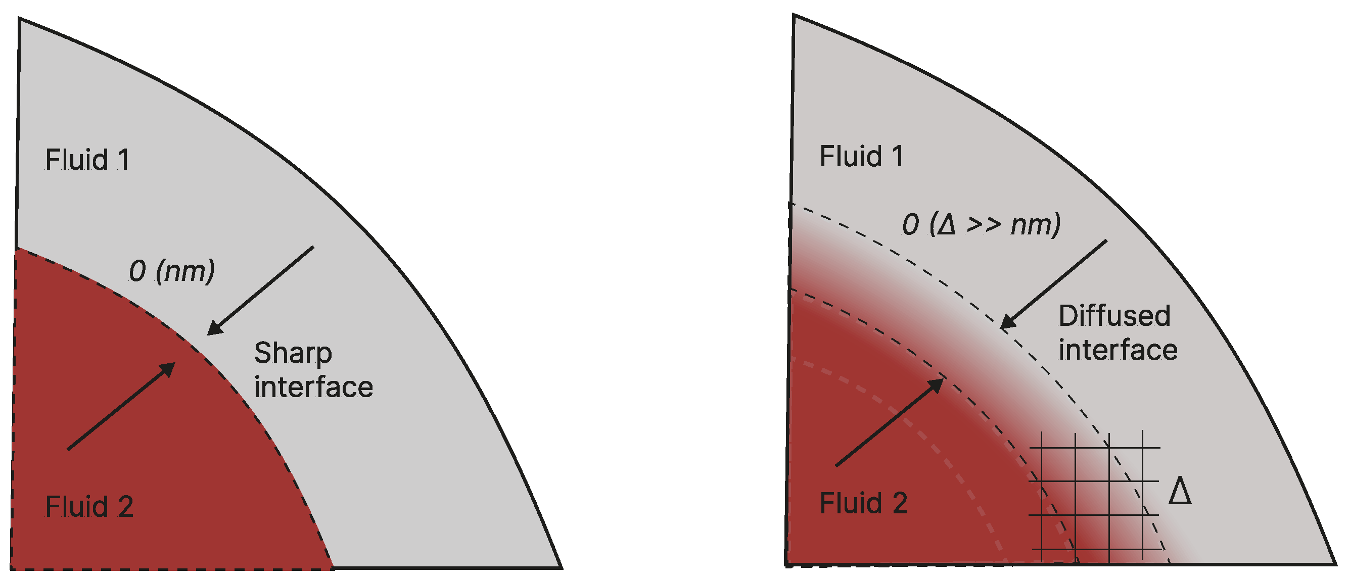
Figure 2.
Diffused-interface models.
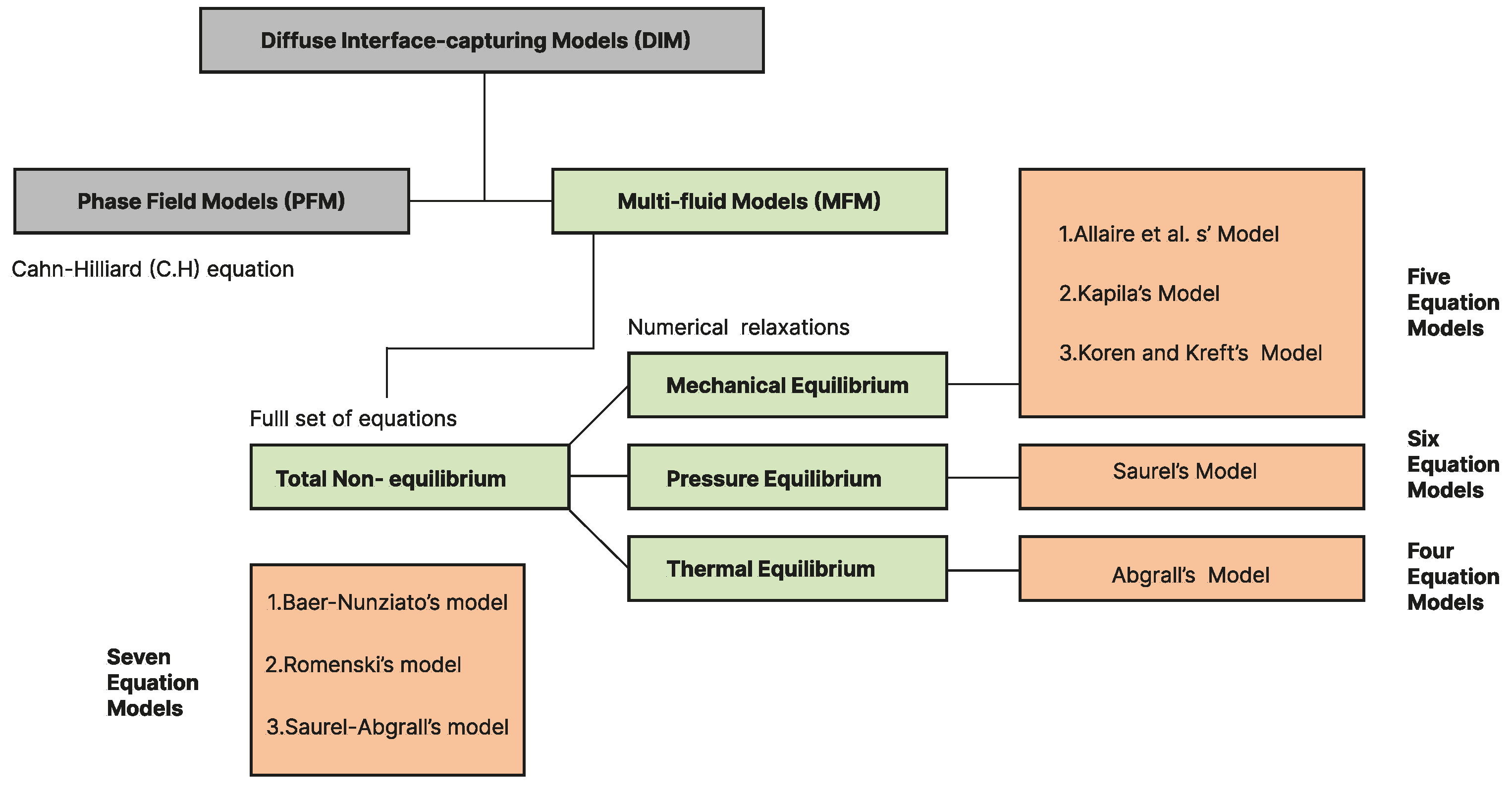
Figure 3.
The hierarchy of seven-equation total disequilibrium models. The Romenski model shares similarities with the B-N-type model (Saurel-Abgrall) for isentropic cases.
Figure 3.
The hierarchy of seven-equation total disequilibrium models. The Romenski model shares similarities with the B-N-type model (Saurel-Abgrall) for isentropic cases.
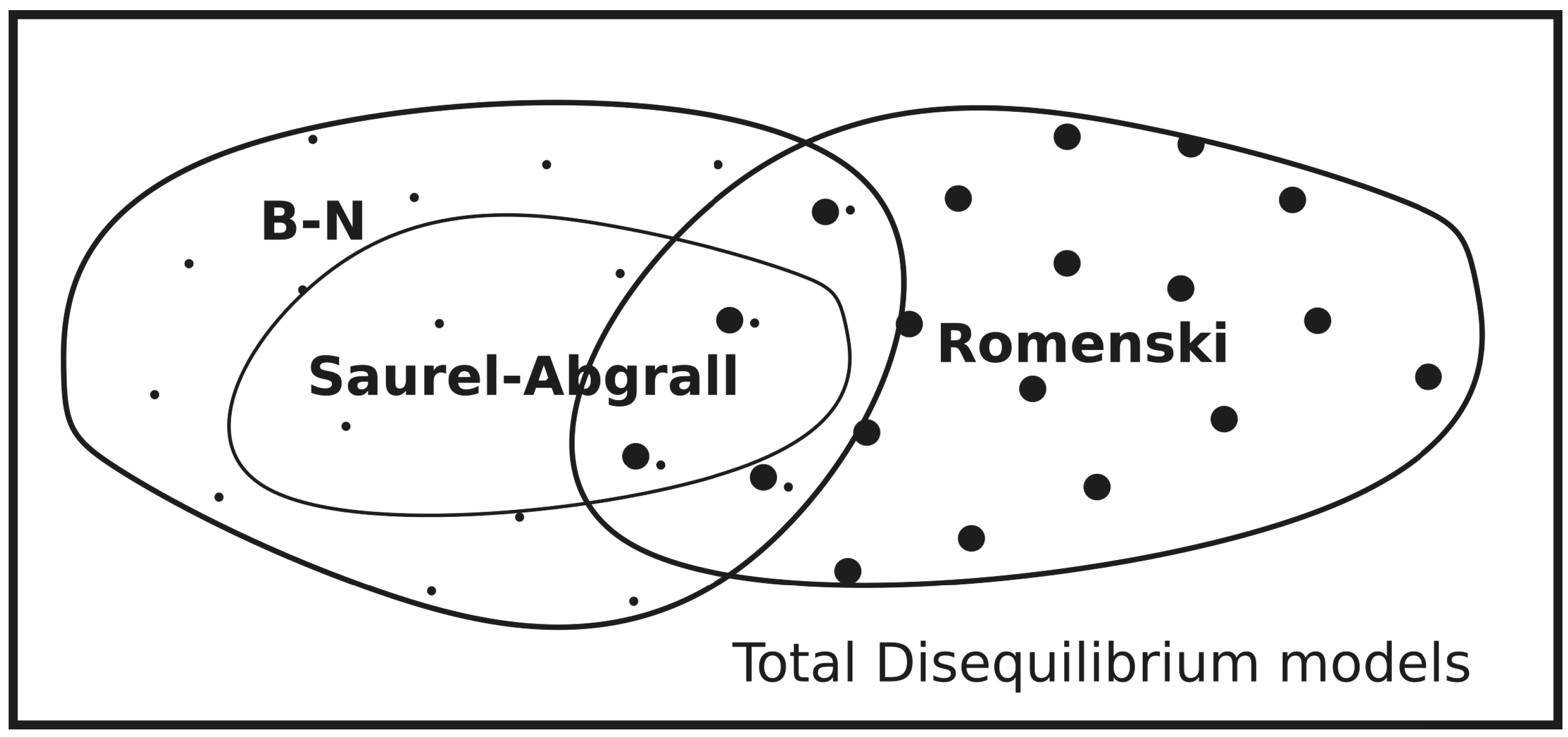
Figure 4.
UNDEX near a free surface; the density gradient contours at different instants, ms . Captured using CWENO4 scheme with fine grid resolution. Source: [125]
Figure 4.
UNDEX near a free surface; the density gradient contours at different instants, ms . Captured using CWENO4 scheme with fine grid resolution. Source: [125]
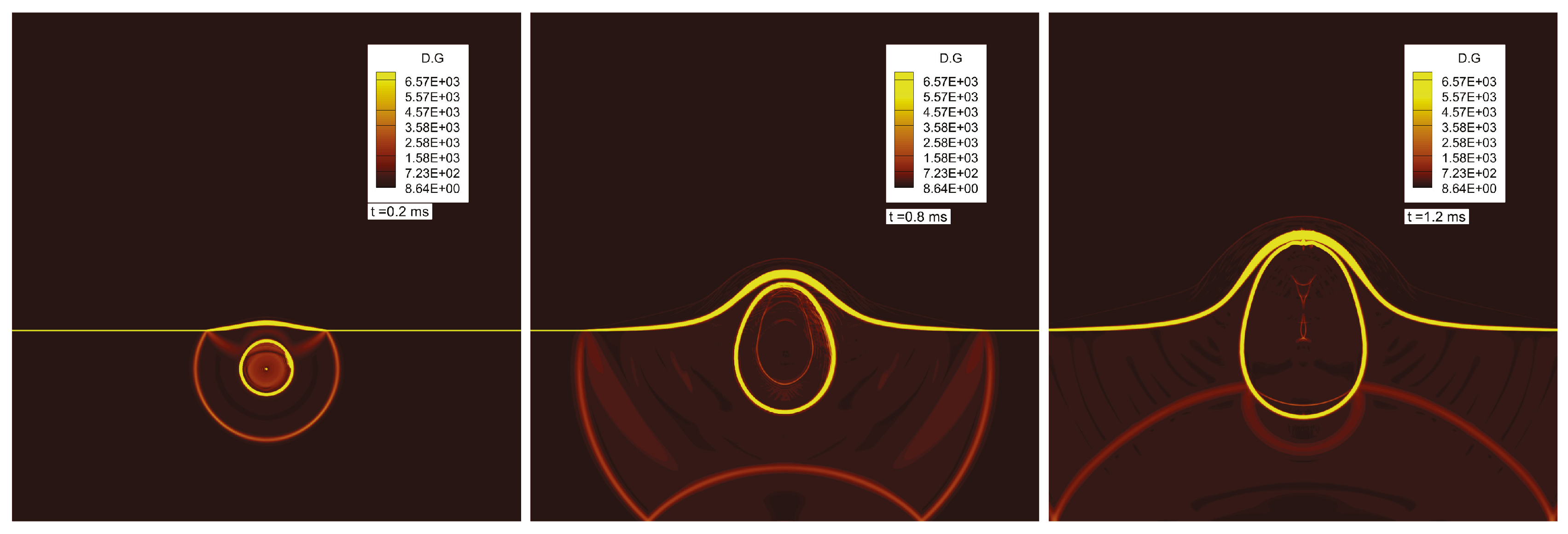
Figure 5.
Predicted bubble and free surface profiles of an underwater explosion using the three flux limiters on the same Grid (300x300). Source: [119]
Figure 5.
Predicted bubble and free surface profiles of an underwater explosion using the three flux limiters on the same Grid (300x300). Source: [119]
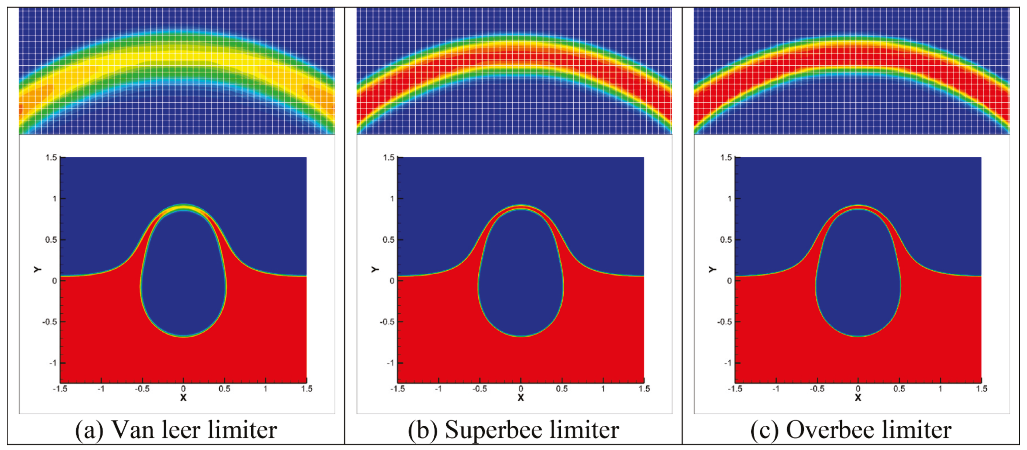
Figure 6.
Water column in the air; Contour plots of density gradient magnitude of the computed solution of the shock wave interaction with a water column with, at various instants Source: [79]
Figure 6.
Water column in the air; Contour plots of density gradient magnitude of the computed solution of the shock wave interaction with a water column with, at various instants Source: [79]
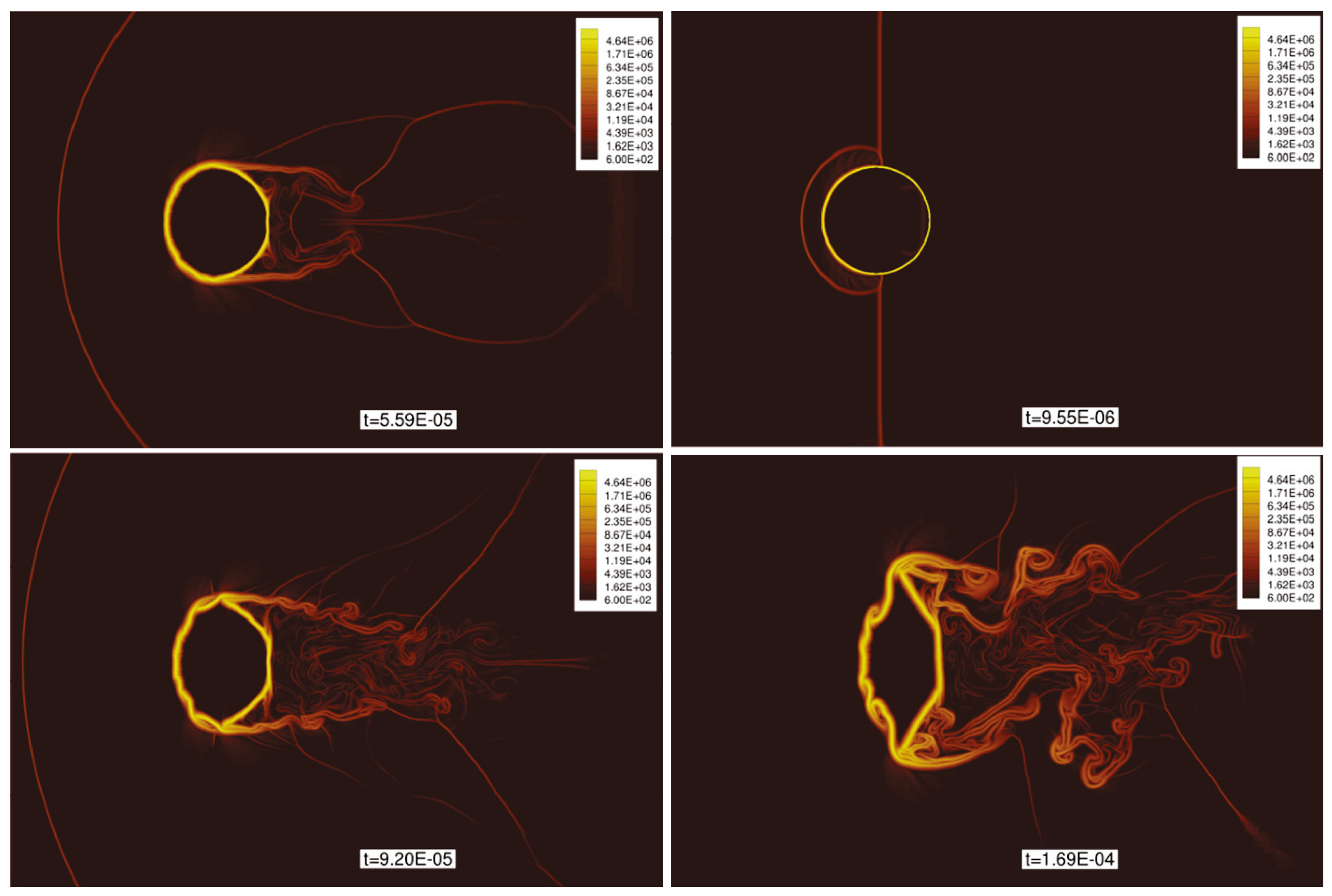
Figure 7.
Contour plots for 3D underwater explosion in an enclosed cylinder. Displayed are the colour maps of density and pressure fields on the central cross-sections and the iso-surface of the volume fraction of 0.5 that represents the moving interface at different instants.
Figure 7.
Contour plots for 3D underwater explosion in an enclosed cylinder. Displayed are the colour maps of density and pressure fields on the central cross-sections and the iso-surface of the volume fraction of 0.5 that represents the moving interface at different instants.
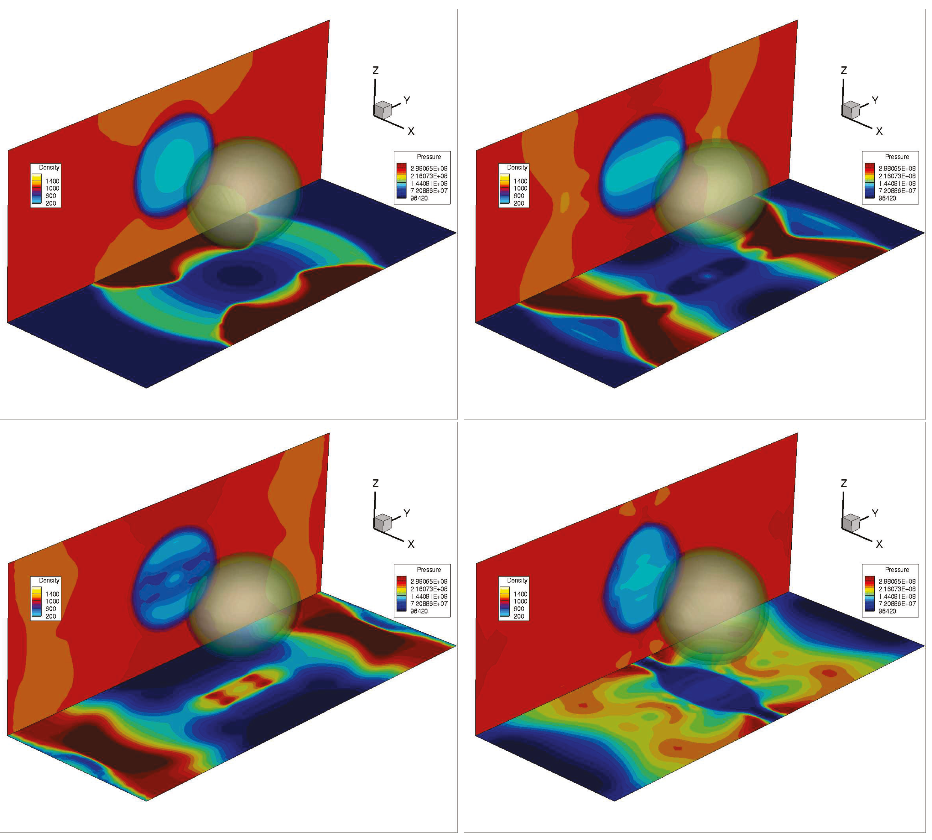
Figure 8.
2D Shock-helium bubble; Colour iso-level plots depicting the volume fraction at employing various mesh resolutions. At this time, the finer grid resolutions effectively capture more vortical structures.
Figure 8.
2D Shock-helium bubble; Colour iso-level plots depicting the volume fraction at employing various mesh resolutions. At this time, the finer grid resolutions effectively capture more vortical structures.
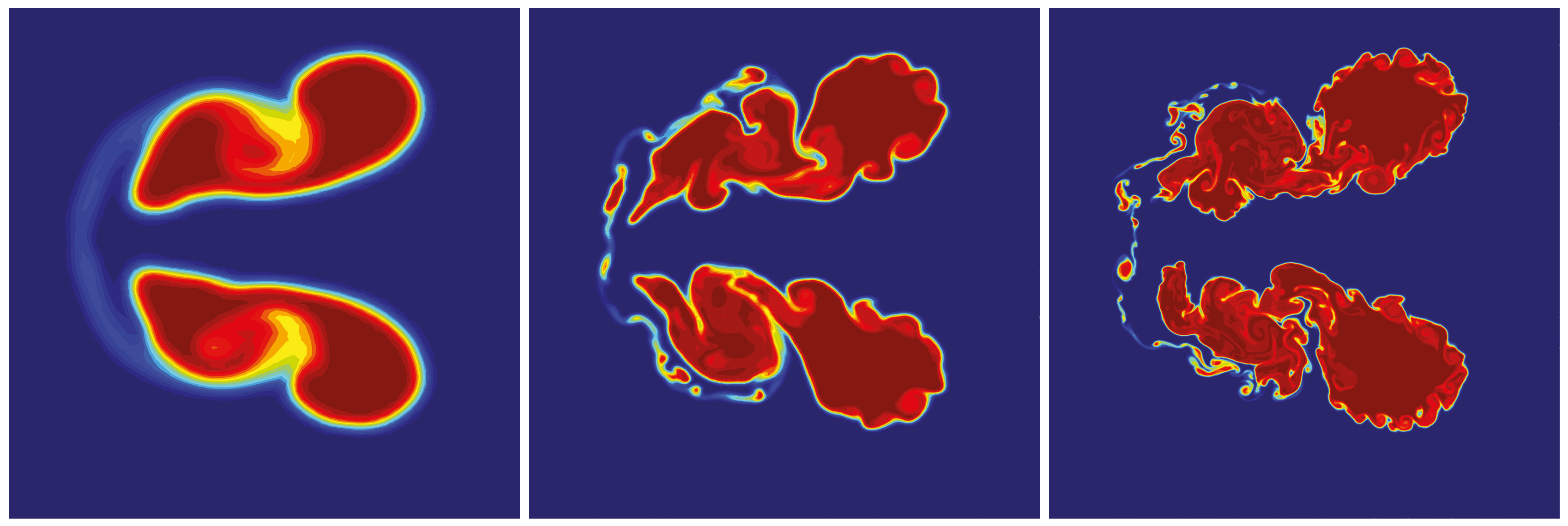
Figure 9.
3D Shock-helium bubble.
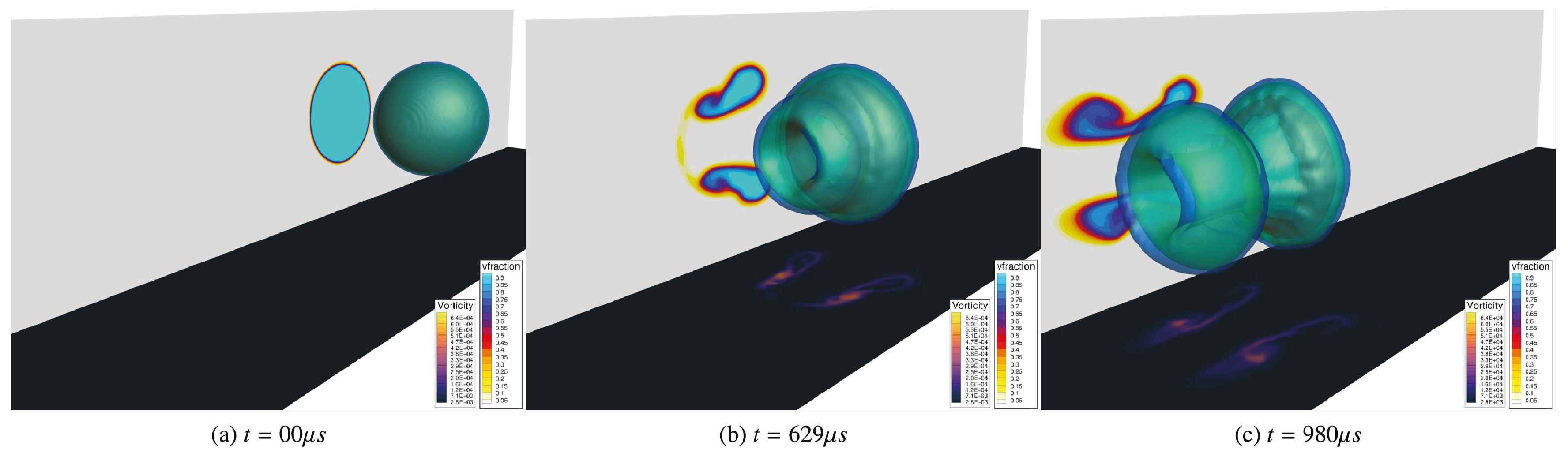
Disclaimer/Publisher’s Note: The statements, opinions and data contained in all publications are solely those of the individual author(s) and contributor(s) and not of MDPI and/or the editor(s). MDPI and/or the editor(s) disclaim responsibility for any injury to people or property resulting from any ideas, methods, instructions or products referred to in the content. |
© 2025 by the authors. Licensee MDPI, Basel, Switzerland. This article is an open access article distributed under the terms and conditions of the Creative Commons Attribution (CC BY) license (http://creativecommons.org/licenses/by/4.0/).
Copyright: This open access article is published under a Creative Commons CC BY 4.0 license, which permit the free download, distribution, and reuse, provided that the author and preprint are cited in any reuse.


