Submitted:
27 January 2025
Posted:
27 January 2025
You are already at the latest version
Abstract
This innovative method improves the inefficient optimization of the parameters of a pneumatic drum seed metering device. The method applies a backpropagation neural network (BPNN) to establish a predictive model and multi-objective particle swarm optimization (MOPSO) to search for the optimal solution. Six types of small vegetable seeds were selected to conduct orthogonal experiments of seeding performance. The results were used to build a dataset for building a BPNN predictive model according to the inputs of the physical properties of the seed (thousand-grain weight, kernel density, sphericity, and geometric mean diameter) and the parameters of the device (vacuum pressure, drum rotational speed, and suction hole diameter). From this, the model output the seeding performance indices (the missing and reseeding indexes). The MOPSO algorithm uses the BPNN predictive model as a fitness function to search for the optimal solution for three types of seeds, and the optimized results were verified through bench experiments. The results show that the predicted qualified indices for tomato, pepper, and bok choi seeds are 85.50%, 85.52%, and 84.87%, respectively. All the absolute errors between the predicted and experimental results are less than 3%, indicating that the results are reliable and meet the requirements for efficient parameter optimization of a seed metering device.
Keywords:
pneumatic drum seed metering device
; backpropagation neural network
; multi-objective particle swarm optimization
; parameter optimization
; physical property
1. Introduction
Due to its adaptability to the shape of seeds, the pneumatic drum seed metering device is widely used. This device provides superior performance when its structural and operational parameters match the properties of the metered seeds. Considerable research has been done on the parameter optimization of pneumatic seed metering devices. Using rice seed, He [2] optimized the intake speed, intake angle, and rotational speed of the suction plate of a pneumatic seed metering device through simulations and bench experiments. Guo [3] designed a pneumatic precision seed metering device with a positive pressure-assisted filling mechanism for peanut seed and optimized its forward speed, vacuum pressure, and positive pressure through bench experiments. Liao [4] optimized the population height and filling chamber structure for a rape seed metering device through simulation and then optimized the vacuum pressure and rotational speed in bench experiments. Each study focused on optimizing parameters for a particular seed, but the results were unsuited to other seed types. A new type of seed required the optimal parameters to be redetermined through inefficient and time-consuming design, simulation, and bench experiments.
Some research on these parameters has been conducted for multiple types of seeds. Davut Karayel’s experiments [5] measured the surface area, thousand-grain weight, kernel density, and sphericity of seven types of seeds and determined the optimal vacuum pressure for each. Then, an artificial neural network was used to establish a predictive model with these physical properties as inputs and the optimal vacuum pressure as output. The model’s accuracy was 99%, indicating that the optimal vacuum pressure can be accurately predicted from a seed’s physical properties. However, the specific seeding performance indices were not obtained directly. Zahra [6] measured the thousand-grain weight, projected area, sphericity, kernel density, and geometric mean diameter of seven types of seeds, conducted performance experiments, and established a regression model using genetic programming, seed properties, and the operational parameters of the seed metering device. The uniformity of seed spacing was output. The coefficient of determination (R2) of the model was 0.938, indicating that the model described the influence of these factors on the uniformity of seed spacing well. However, the model accuracy was not verified by seeds other than the experimental seeds, nor was the model further used for parameter optimization.
To improve the efficiency of the parameter optimization, this study used the physical properties of seeds and the device parameters as inputs to establish a suitable predictive model to optimize the parameters and output the seeding performance indices.
Machine learning has begun to be applied in agriculture. Machine learning techniques, including artificial neural networks (ANNs), random forest (RF), adaptive boosting (AdaBoost), support vector regression (SVR), and extreme learning machine (ELM), have been used for modeling in parameter optimization [7,8,9,10]. Na [11] and M. Anantachar [12] used regression analysis and ANNs to demonstrate that an ANN model has better predictive accuracy than the statistical models of traditional regression analysis. Their high learning and information-processing ability make them suitable for complex nonlinear modeling [13].
The methods to optimize parameters from a model must be specific, and multi-objective methods are needed for problems with multiple objectives. Pareek [14] used the multi-objective particle swarm optimization (MOPSO) algorithm to optimize the qualified index and seed spacing variation index of a seed metering device; Yang [15] used non-dominated sorting genetic algorithm II (NSGA-II) to optimize the residual stress and Vickers hardness of the WC-10Co-4Cr coating. Meta-heuristic search algorithms, such as MOPSO and NSGA-II, are widely used in multi-objective optimization. Compared to other multi-objective optimization algorithms, the MOPSO algorithm has fewer adjustment parameters, faster convergence speed, and uniform Pareto optimal frontier distribution [14], suitable for further parameter optimization study.
This paper consists of three parts:
- A discussion of the dataset required for ANN training through seeding performance experiments;
- An explanation of using backpropagation neural network (BPNN) to establish a predictive model of seeding performance from the input physical properties of seeds (geometric mean diameter, sphericity, thousand-grain weight, and kernel density), operational parameters (vacuum pressure and drum rotational speed), and structural parameters (suction hole diameter), producing seeding performance indices (missing index and reseeding index);
- A description of optimization method of the combination of the BPNN predictive model and MOPSO algorithm (BPNN-MOPSO) to search for optimal device parameters, with the lowest missing and reseeding indexes as the optimization objectives.
2. Materials and Methods
2.1. Overall Structure and Working Principle
Figure 1 shows the structure of the tested pneumatic drum seed metering device. The lugs at the ends fasten the air intake plate to the frame. One end of the drum is fitted with this plate to enable relative rotation, with the other embedded in the end cover and a rubber sealing ring at each end. The end cover is connected to the drive shaft with a flat key and transfers the shaft’s rotational motion.
The fan exhausts air through the negative pressure port, creating a vacuum inside the drum. The pressure difference pulls seeds into moving suction holes as they pass the seed box. Positive air pressure then blows the unstably adsorbed seeds into the seed recycling bin. When the suction holes pass a pressure isolation roller, the vacuum is isolated, air pressure is applied, and the adsorbed seeds are blown onto the plug tray.
2.2. Influencing Factors and Seeding Performance Indices
The factors in this process are the hole diameter, vacuum pressure, and drum rotational speed. The seeding performance indices are the missing index (MI), the reseeding index (RI), and the qualified index (QI). MI is the percentage of holes with no seed. RI is the percentage of holes with more than two seeds. QI is the percentage of holes with one or two seeds. The expressions for MI, RI, and QI are as follows:
where N1 is the number of holes with no seeds; N2 is the number of holes with more than two seeds; N3 is the number of holes with one or two seeds; and N is the total number of holes.
2.3. Value Range of Factors
Considering the geometric mean diameter of six types of seeds, the range of suction hole diameter was determined to between 0.6 and 1.0 mm. A previous study [16] showed that a drum speed between 10 and 14 rpm was suitable. The vacuum pressure was set according to the seed type, thus single-factor vacuum pressure experiments were conducted. The hole diameter and drum speed were set to 0.8 mm and 12 rpm, respectively. Figure 2 presents the test results.
2.4. Orthogonal Experiments
Orthogonal experiments with three factors and three levels were designed using Design-Expert 13. Table 2 shows the factor level settings.
2.5. Predictive Model Using Backpropagation Neural Network
BPNN is widely applied in regression problems [17,18,19,20,21,22,23,24]. This study used a BPNN to determine the relationships between the suction hole diameter, vacuum pressure, drum rotational speed, physical properties of seed types, and seeding performance.
2.5.1. Seeding Performance Dataset
To complete the dataset, we measured the geometric mean diameter (Dg), sphericity (ϕ), thousand-grain weight (m1000), and kernel density (ρs) of six seed types. The length (L), width (W), and height (T) of the seeds were measured with an electronic vernier caliper. The thousand-grain weight of the seeds was measured with an electronic scale. The kernel density was determined by the pycnometer method, shown in Figure 3.
The computational formulas for the seed’s physical properties are as follows:
where ρw is the density of water. Table 9 lists the physical properties.
The physical property data were merged into the dataset to form a complete dataset, which was then divided into a training set and a test set in an 8:2 ratio, with 72 and 18 data groups, respectively. To ensure the validity of the test set, three data groups were randomly selected from each seed’s experimental data to constitute the test set, as shown in Table 10. The remaining data were used as the training set.
2.5.2. Backpropagation Neural Network
A BPNN uses forward information and backward error correction propagation. It typically has a three-layer structure comprising input, hidden, and output layers [25]. The input layer neurons play a role in information transmission. BPNN-predicted results are obtained by applying the activation functions of the hidden and output layers to the weighted sum of the previous layer’s inputs, as follows [13]:
where is kth output variable, and and are activation functions of the output layer and hidden layer, respectively; i, j, and k are the neurons of the input layer, the hidden layer, and the output layer, respectively, and given as i = 1, 2, …, m; j = 1,2,…,n; and k = 1, 2, …, l. Wij is the connection weight between the ith neuron in the input layer and the jth neuron in the hidden layer; Ujk is the connection weight between the jth neuron in the hidden layer and the kth neuron in the output layer; (bh)j is the bias for the jth neuron in the hidden layer; and (bo)k is the bias for the kth neuron in the output layer.
2.5.3. Evaluation Indices for Network Performance
The coefficient of determination (R2), root mean square error (RMSE), and mean absolute error (MAE) served as evaluation indices for BPNN’s predictive performance. R2 indicates the degree of fitting of the predictive model: the closer its value is to 1, the more accurate the predicted results. RMSE and MAE evaluate the error of the predictive model. The closer their values are to 0, the smaller the predictive error. The expressions for R2, RMSE, and MAE are as follows [26,27,28]:
where Yei is the experimental value for the ith sample, i = 1, 2, …, n, where n is the total number of samples. Ypi is the predicted value for the ith sample, and is the average of experimental values for all samples.
2.5.4. Establishment of BPNN Predictive model
The BPNN predictive model was established using the newff function in MATLAB R2022a. To ensure the model’s accuracy, the sample data were normalized before use [29]. This paper normalized the data within [0, 1], as follows:
The settings of network training parameters are shown in Table 11. The network structure parameters, such as the number of hidden-layer neurons and the activation functions of the hidden and output layers, must be determined through tests.
According to the independent and dependent variables of the dataset, the numbers of input and output layer neurons were set to 7 and 2, respectively. The number of hidden-layer neurons is not a constant value, which was preliminarily determined within [4,13] as follows [30]:
where p is the number of hidden-layer neurons; m is the number of input variables; n is the number of output variables; and A is a constant in [1,10].
2.6. BPNN-MOPSO Parameter Optimization of the Seed Metering Device
2.6.1. Principle and Flow of the MOPSO Algorithm
The MOPSO principle is the same as that of PSO and originates from the group behavior of foraging birds. When a bird finds food, others gather around to search for food [31]. PSO searches for the extremum of a single optimization objective. Unlike PSO, MOPSO searches for a Pareto optimal set consisting of non-dominated solutions for multiple optimization objectives.
The main flow of the MOPSO algorithm is as follows:
- Define a fitness function based on optimization objectives, determine the dimensions and constraints for each input variable, and set MOPSO algorithm parameters;
- Randomly generate position and velocity vectors for the initial population; then, calculate and record the fitness value of each particle as the individual optimal value;
- Based on Pareto dominance, check the dominance relationship of all particles, record all non-dominated solutions, and select one as the global optimal value;
- Update the velocity and position vectors of the population, recalculate each particle’s fitness value, recheck the domination relationship, and update the non-domination solution library;
- Update individual and global optimal values;
- Check whether the maximum number of iterations is reached. If so, the algorithm terminates; otherwise, return to Step 4;
- Output the Pareto optimal set and the Pareto optimal front.
2.6.2. Settings of the MOPSO Algorithm Parameters
The settings of the MOPSO algorithm parameters are shown in Table 12.
2.6.3. Mathematical Model for the Multi-objective Optimization Problem
With minimal MI and RI as optimization objectives, and based on the constraint conditions of suction hole diameter, vacuum pressure, and drum rotational speed, a mathematical model for the multi-objective optimization problem was established, as follows:
where a, b, c, and d are the geometric mean diameter (mm), sphericity (%), thousand-grain weight (g), and kernel density (g·cm-3) of seeds, respectively; x1, x2, and x3 are the suction hole diameter (mm), vacuum pressure (kPa), and drum rotational speed (rpm), respectively; f1(x) and f2(x) are the prediction functions of MI and RI, respectively. Table 13 shows the values of e and f, which represent the lower and upper limits of the vacuum pressure, respectively, and g and h represent the lower and upper limits of the drum rotational speed, respectively.
2.6.4. Scoring Method for Solutions
To select a solution from the Pareto optimal set as the optimization result, we had to assign corresponding weights to the optimization objectives, score each solution, and select the one with the highest score as the final result. To ensure a highly qualified index for the seed metering device, the QI is also taken as an optimization objective and given a corresponding weight. The weights of the QI, MI, and RI were set to 0.6, 0.3, and 0.1, respectively. The indices were normalized before scoring. The normalization formulas for the positive index (QI) and negative index (MI and RI) and the scoring formula are as follows:
where xij is the jth sample of the ith index, where i = 1, 2, …, m, j = 1, 2, …, n, m is the total number of indices, n is the total number of solutions in the Pareto optimal set; ωi is the weight of the ith index.
2.6.5. Process of BPNN-MOPSO
After network training, the optimal BPNN predictive model served as the fitness function in MOPSO. Then, the MOPSO algorithm searched for the optimal solution predicted by the BPNN predictive model. The BPNN-MOPSO process is shown in Figure 4. Before running the BPNN-MOPSO algorithm, the first four dimensions of the particles were fixed as the physical properties for each seed type. Thus, during algorithm execution, the BPNN predictive model becomes a seeding performance predictor for the seed type, then is used to optimize the device parameters.
3. Results and Discussion
3.1. Determination of the Number of Hidden-Layer Neurons
The network was trained and tested to determine the optimal number of hidden-layer neurons, successively setting the number of hidden-layer neurons as integers in [4,13]. Owing to the characteristics of the gradient descent method, a BPNN tends to fall into local minima during training and may result in the trained network not achieving optimal performance [32,33]. Moreover, since the gradient descent path is not unique, the BPNN training is unstable [15], which means the network trained each time is inconsistent. Under each number of hidden-layer neurons, network training was repeated until 10 sets of network performance data with two output’s test set R2 values simultaneously greater than 0.8 were obtained. Then, the optimal set of data was selected from the 10 sets of data to represent the network performance under the current number of hidden-layer neurons. The network performance data were compared, as shown in Figure 5 and Table 14.
With eight hidden-layer neurons, network performance is excellent. Except that the test set is slightly larger than that obtained with 4–7 neurons, the other performance indices are the optimal values. Thus, the number of hidden-layer neurons was set to 8.
3.2. Determination of the Activation Functions for the Hidden and Output Layers
Commonly used activation functions of hidden and output layers include logsig, tansig, and purelin. Therefore, the optimal activation function combination was determined by comparing network performance under all combinations of the three activation functions. Since the R2 values of the two outputs were negative when the output layer activation function was logsig, combinations with logsig as the output layer activation function were excluded. The training results of the remaining combinations are shown in Figure 6 and Table 15.
Network performance is better for the logsig/purelin combination. Except that the training set is slightly smaller than that of the tansig/purelin combination, the other network performance indices are the optimal values. Thus, the optimal activation function combination of the hidden and output layers was set to logsig/purelin.
3.3. Determination of the Optimal BPNN Performance
The network structure parameters were determined, and then the BPNN was trained. After multiple network training, the networks with excellent performance were saved, and the network performance data were recorded. All network performance data were compared, and the optimal network was selected for subsequent research. The performance of the selected network is shown in Figure 7, Figure 8, and Table 16.
The weights and biases of the optimal performance BPNN were extracted for the further combination of the BPNN predictive model and MOPSO algorithm, as shown in Table 17.
3.4. Verification of Optimization Capability of BPNN-MOPSO
3.5. BPNN-MOPSO Optimization Results and Experimental Verification
Using the BPNN-MOPSO algorithm, the device parameters for tomato, pepper, and bok choi seeds were optimized. Then, the optimization results were verified through bench experiments to prove the algorithm’s validity for efficient parameter optimization. The physical properties of the three types of seeds are shown in Table 19.
The algorithm found the Pareto optimal set. The Pareto optimal frontiers of the three types of seeds are shown in Figure 10.
The 100 non-dominated solutions for each seed type were scored, and the solution with the highest score was recorded as the optimized result. The results are shown in Table 20.
The bench experiments were carried out to verify the optimization results in Table 20, and the verification results are shown in Table 21.
According to Table 21, the predicted qualified indices for tomato, pepper, and bok choi seeds are all greater than 80%, which are 85.50%, 85.52%, and 84.87%, respectively. All the absolute errors are less than 3%. The verification results prove the accuracy of the established BPNN predictive model and the effectiveness of the MOPSO algorithm for searching for the optimal solution, showing that the parameter optimization method based on the BPNN/MOPSO combination simplifies the parameter optimization process effectively, improves optimization efficiency, and shortens research time.
4. Conclusions
(1) Considering the geometric mean diameters of carrot, sesame, onion, cabbage, Chinese cabbage, and radish seeds, the range of suction hole diameter was determined to be from 0.6 to 1.0 mm. The range of drum rotational speed was from 10 to 14 rpm according to a previous study. The vacuum pressure single-factor experiments showed that the suitable vacuum pressure range was from 6 to 10 kPa for Chinese cabbage, carrot, sesame, and onion, from 8 to 12 kPa for cabbage, and from 10 to 14 kPa for radish seeds. The three factors and three levels of orthogonal experiments were investigated to obtain the seeding performance data. The four physical properties of the six kinds of seeds were measured and merged into the seeding performance dataset, completing the dataset required for BPNN training.
(2) The optimal number of hidden-layer neurons and the optimal activation function for the hidden and output layers were determined through tests, which were 8 and logsig/purelin, respectively. Next, network training was used to determine the optimal BPNN performance.
(3) Determine the minimum MI and RI as the optimization objectives, the BPNN predictive model and MOPSO algorithm were combined to search for the optimal device parameters and seeding performance for cabbage, carrot, radish, onion, Chinese cabbage, and sesame seeds. The QIs of the optimization results were higher than those of the optimal experimental results, and the increased QIs for cabbage, carrot, radish, onion, Chinese cabbage, and sesame seeds were 1.55%, 1.43%, 0.59%, 1.87%, 0.22%, and 2.53%, respectively. These results show that BPNN-MOPSO can optimize seeding performance.
(4) Using the BPNN-MOPSO algorithm, the optimal device parameters and seeding performance for tomato, pepper, and bok choi seeds were sought. For tomato seeds, with a hole diameter of 0.75 mm, vacuum pressure of 5.6 kPa, and drum rotational speed of 13.7 rpm, the MI, RI, and QI were 11.85%, 2.66%, and 85.50%, respectively. For pepper seeds, with a hole diameter of 1.0 mm, vacuum pressure of 10.4 kPa, and drum rotational speed of 18.0 rpm, the MI, RI, and QI were 11.54%, 2.94%, and 85.52%, respectively. For bok choi, with a hole diameter of 0.67 mm, vacuum pressure of 8.6 kPa, and drum rotational speed of 14.0 r·min-1, the MI, RI, and QI were 10.72%, 4.41%, and 84.87%, respectively. The bench experiments verified the optimization results. The results show that the absolute error between the predicted and experimental values was less than 3%, indicating that the BPNN predictive model and MOPSO algorithm provided reliable parameter optimization results and effectively improved the efficiency of parameter optimization for the tested seed metering device.
Author Contributions
Conceptualization, Y.P. and Y.Y.; methodology, Y.P. and Y.Y.; software, Y.P.; validation Y.P., J.Z. and Y.W.; formal analysis, Y.P.; investigation, Y.P., J.Z., W.Q. and Q.W.; data curation, Y.P.; writing—original draft preparation, Y.P.; writing—review and editing, Y.P. and Y.Y.; project administration, Y.P. and Y.Y.; funding acquisition, Y.Y. All authors have read and agreed to the published version of the manuscript.
Funding
This research was supported by National Natural Science Foundation of China (Grant No. 51975538) and The Key Research and Development Program of Zhejiang Province (No.2023C02011).
Institutional Review Board Statement
Not applicable.
Data Availability Statement
Data will be made available upon reasonable request.
Acknowledgments
The authors would like to thank their school and all the colleagues who have contributed to the research work.
Conflicts of Interest
The authors declare no conflicts of interest.
References
- Chen, H.T.; Li, T.H.; Wang, H.F.; Wang, Y.; Wang, X. Design and parameter optimization of pneumatic cylinder ridge three-row close-planting seed-metering device for soybean. Transactions of the Chinese Society of Agricultural Engineering 2018, 34, 16–24.
- He, X.; Cao, X.M.; Peng, Z.; Wan, Y.K.; Lin, J.J.; Zang, Y.; Zhang, G.Z. DEM-CFD Coupling Simulation and Optimization of Rice Seed Particles Seeding a Hill in Double Cavity Pneumatic Seed Metering Device. Computers and Electronics in Agriculture 2024, 224, 109075. [CrossRef]
- Guo, P.; Zheng, X.S.; Wang, D.W.; Hou, J.L.; Zhao, Z. Design and Experiment of Precision Seed Metering Device with Pneumatic Assisted Seed-filling for Peanut. Transactions of the Chinese Society for Agricultural Machinery 2024, 55, 64–74.
- Liao, Y.T.; Liu, J.C.; Liao, Q.X.; Zheng, J.; Li, T.; Jiang, S. Design and Test of Positive and Negative Pressure Combination Roller Type Precision Seed-metering Device for Rapeseed. Transactions of the Chinese Society for Agricultural Machinery 2024, 55, 63–76.
- Karayel, D.; Güngör, O.; Šarauskis, E. Estimation of Optimum Vacuum Pressure of Air-Suction Seed-Metering Device of Precision Seeders Using Artificial Neural Network Models. Agronomy 2022, 12, 1600. [CrossRef]
- Abdolahzare, Z.; Mehdizadeh, S.A. Nonlinear Mathematical Modeling of Seed Spacing Uniformity of a Pneumatic Planter Using Genetic Programming and Image Processing. Neural Comput & Applic 2018, 29, 363–375. [CrossRef]
- Zhou, X.L.; Qin, N.; Wang, K.Y.; Sun, H.; Wang, D.W.; Qiao, J.Y. Effect of Mechanical Compaction on Soybean Yield Based on Machine Learning. Transactions of the Chinese Society for Agricultural Machinery 2023, 54, 139–147.
- Chen, S.M.; Li, X.L.; Yang, Q.L.; Wu, L.F.; Xiong, K.; Liu, X.G. Estimation of reference evapotranspiration in shading facility using machine learning. Transactions of the Chinese Society of Agricultural Engineering 2022, 38, 108–116.
- Zhang, Y.F.; Pan, Z.Q.; Chen, D.J. Estimation of Cropland Nitrogen Runoff Loss Loads in the Yangtze River Basin Based on the Machine Learning Approaches. Environmental Science 2023, 44, 3913–3922. [CrossRef]
- Jiang, Z.W.; Yang, S.H.; Liu, Z.Y.; Xu, J.Z.; Pang, Q.Q.; Using Machine Learning to Predict Water level in the Drainage Sluice Stations Following Rainfalls. Journal of Irrigation and Drainage 2022, 41, 135–140. [CrossRef]
- Na, X.Y.; Zhao, C.Y.; Sun, S.M.; Zhang, Z.G. Performance test and forecast analysis for air suction seed metering device. Journal of Hunan Agricultural University (Natural Sciences) 2015, 41, 440–442.
- Anantachar, M.; Kumar, P.G.V.; Guruswamy, T. Neural Network Prediction of Performance Parameters of an Inclined Plate Seed Metering Device and Its Reverse Mapping for the Determination of Optimum Design and Operational Parameters. Computers and Electronics in Agriculture 2010, 72, 87-98. [CrossRef]
- Roy, S.M.; Pareek, C.M.; Machavaram, R. Optimizing the Aeration Performance of a Perforated Pooled Circular Stepped Cascade Aerator Using Hybrid ANN-PSO Technique. Information Processing in Agriculture 2022, 9, 533-546. [CrossRef]
- Pareek, C.M.; Tewari, V.K.; Machavaram, R. Multi-Objective Optimization of Seeding Performance of a Pneumatic Precision Seed Metering Device Using Integrated ANN-MOPSO Approach. Engineering Applications of Artificial Intelligence 2023, 117, 105559. [CrossRef]
- Yang, Y. Study on WC-10Co-4Cr Coating Prediction Model and Multi-objective Optimization by High Velocity Oxy-Fuel spraying Based on Neural Network. Master’s Thesis, Zhejiang University, Hangzhou, China, 2023.
- Ke, S.D. Research on virtual prototype of pneumatic drum seed metering device based on seed characteristics. Master’s Thesis, Zhejiang Sci-Tech University, Hangzhou, China, 2022.
- Du, Y.; Li, X.H.; Cao, L.M.; Yang, J. One-Step Solvothermal Synthesis of MoS2@Ti Cathode for Electrochemical Reduction of Hg2+ and Predicting BP Neural Network Model. Separation and Purification Technology 2024, 331, 125654. [CrossRef]
- Zhao, P.; Zeng, X.G.; Kou, H.Q.; Chen, H.Y. A Kind of Numerical Model Combined with Genetic Algorithm and Back Propagation Neural Network for Creep-Fatigue Life Prediction and Optimization of Double-Layered Annulus Metal Hydride Reactor and Verification of ASME-NH Code. International Journal of Hydrogen Energy 2024, 54, 1251–1263. [CrossRef]
- Liu, J.F.; He, X.; Huang, H.Y.; Yang, J.X.; Dai, J.J.; Shi, X.C.; Xue, F.J.; Rabczuk, T. Predicting Gas Flow Rate in Fractured Shale Reservoirs Using Discrete Fracture Model and GA-BP Neural Network Method. Engineering Analysis with Boundary Elements 2024, 159, 315–330. [CrossRef]
- Guo, J.W.; Huang, Y.Q.; Li, Z.Y.; Li, J.R.; Jiang, C.; Chen, Y.R. Performance Prediction and Optimization of Lateral Exhaust Hood Based on Back Propagation Neural Network and Genetic Algorithm. Sustainable Cities and Society 2024, 113, 105696. [CrossRef]
- Chen, C.; Wang, X.S.; Pu, J.; Jiao, S.S. Kinetic Analysis and Back Propagation Neural Network Model for Shelf-Life Estimation of Stabilized Rice Bran. Journal of Food Engineering 2024, 380, 112168. [CrossRef]
- Guo, Y.H.; Wang, S.C.; Liu, G. Creep–Fatigue Life Prediction of a Titanium Alloy Deep-Sea Submersible Using a Continuum Damage Mechanics-Informed BP Neural Network Model. Ocean Engineering 2024, 311, 118826. [CrossRef]
- Liu, Y.H. Prediction of Seawater Desalination Reverse Osmosis Membrane Contamination Based on BP Neural Network Model. Master’s Thesis, Qingdao University of Technology, Qingdao, China, 2023.
- Lyu, B.N. Research on design and performance prediction of composite recycled powder mortar based on artificial neural network. Master’s Thesis, Shandong University, Jinan, China, 2023.
- Yao, S.C.; Li, D.W. Neural network and deep learning: simulation and realization based on MATLAB, 1st ed.; Tsinghua University Press: Beijing, China, 2022; pp. 118.
- Fan, X.Y.; Lyu, S.T.; Xia, C.D.; Ge, D.D.; Liu, C.C.; Lu, W.W. Strength Prediction of Asphalt Mixture under Interactive Conditions Based on BPNN and SVM. Case Studies in Construction Materials 2024, 21, e03489. [CrossRef]
- Li, W.; Kuang, C.W.; Chen, Y.X. Prediction Model of Soil Moisture in Hainan Island Based on Meteorological Factors. Chinese Journal of Tropical Agriculture 2023, 43, 84-89.
- Yao, X.W.; Zhang, L.Y.; Xu, K.L.; Qi, Y. Study on neural network-based prediction model for biomass ash softening temperature. Journal of Safety and Environment 2024, 24, 3801–3808.
- Li, A.L.; Zhao, Y.M.; Cui, G.M.; Study on Temperature Prediction Model of Blast Furnace Hot Metal Based on Data Preprocessing and Intelligent Optimization. FOUNDRY TECHNOLOGY 2015, 36, 450–454.
- Lin, X.Z.; Wang, H.; Guo, L.L.; Yan, D.M.; Li, L.J.; Liu, Y.; Sun, J. Prediction Model of Laser 3D Projection Galvanometer Deflection Voltage Based on PROA-BP. ACTA PHOTONICA SINICA 2024, 53, 56–68.
- Li, J. Study on reliability evaluation of artillery servo system based on particle swarm optimization algorithm. Master’s Thesis, Xi’an Technological University, Xi’an, China, 2023.
- Xu, J.H. Research on ship personnel evacuation time prediction model based on neural network. Master’s Thesis, Dalian Ocean University, Dalian, China, 2024.
- Wang, Y.J. Research on grinding roughness value prediction method based on improved GA-BP. Master’s Thesis, Hebei Normal University of Science & Technology, Qinghuangdao, China, 2024.
Figure 1.
Pneumatic drum seed meter: (a) overall structure; (b) explosion diagram of the drum; (c) bench; (1) drive shaft, (2) end cover, (3) drum, (4) rubber sealing ring, (5) air intake plate, (5-1) negative pressure port, (5-2) positive pressure port, (5-3) pressure isolation roller, (6) seed box, (7) seed cleaning device, (8) seed recycling bin, (9) electrical machinery, (10) fan, and (11) air compressor.
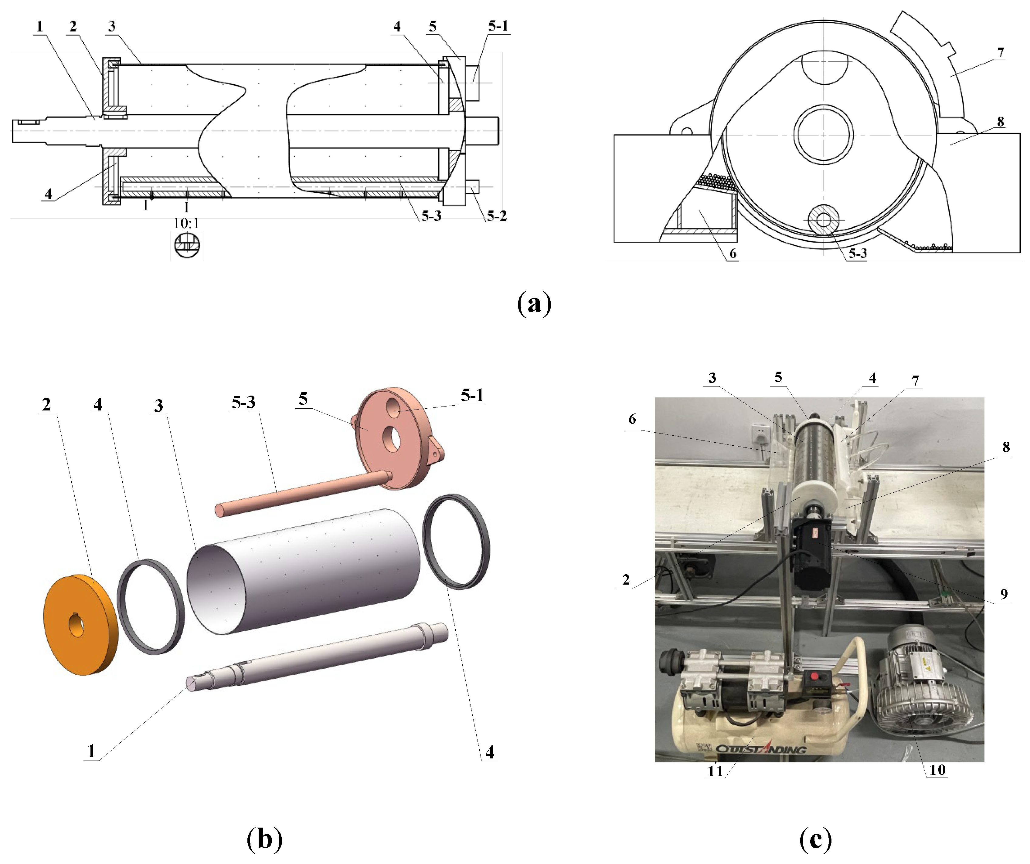
Figure 2.
Results of the single-factor vacuum pressure experiments for (a) Chinese cabbage; (b) carrot; (c) sesame; (d) onion; (e) cabbage; and (f) radish seed (QI, MI, and RI denote qualified index, missing index, and reseeding index, respectively).
Figure 2.
Results of the single-factor vacuum pressure experiments for (a) Chinese cabbage; (b) carrot; (c) sesame; (d) onion; (e) cabbage; and (f) radish seed (QI, MI, and RI denote qualified index, missing index, and reseeding index, respectively).
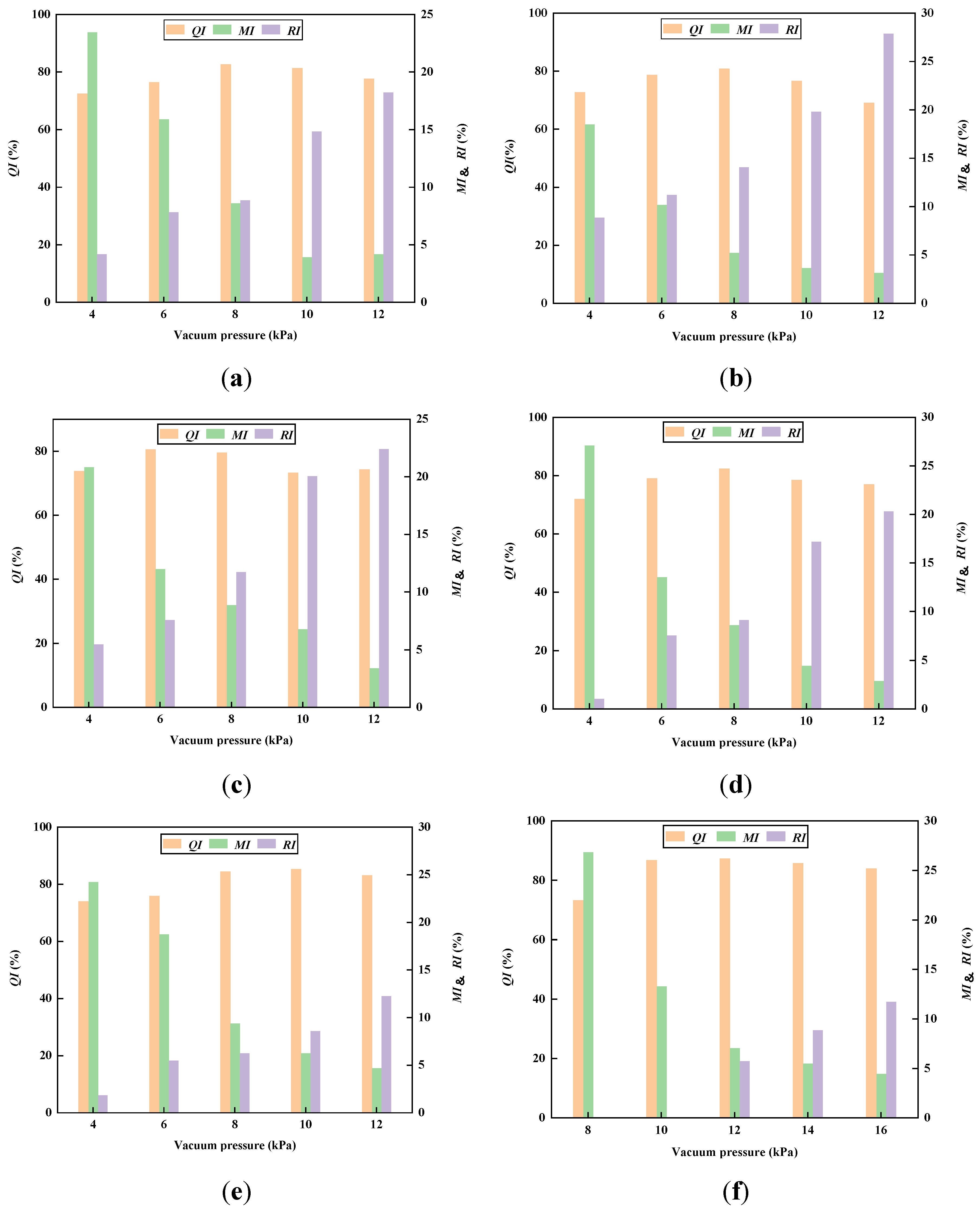
Figure 3.
Kernel density determination by pycnometer method: (a) weight of seeds (m1); (b) weight of water and pycnometer (m2); (c) weight of seeds, water, and pycnometer (m3).
Figure 3.
Kernel density determination by pycnometer method: (a) weight of seeds (m1); (b) weight of water and pycnometer (m2); (c) weight of seeds, water, and pycnometer (m3).
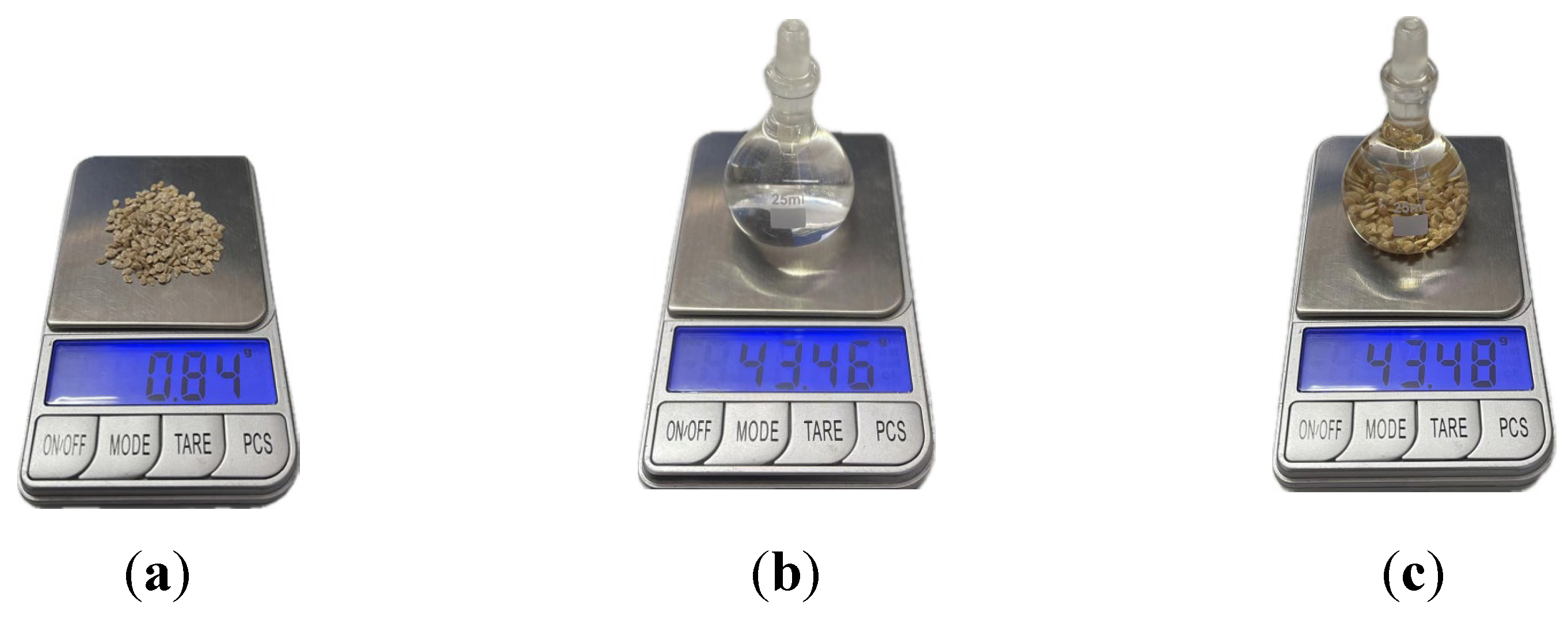
Figure 4.
BPNN-MOPSO process (BPNN-MOPSO denotes optimization method of the combination of the backpropagation neural network (BPNN) predictive model and multi-objective particle swarm optimization (MOPSO) algorithm).
Figure 4.
BPNN-MOPSO process (BPNN-MOPSO denotes optimization method of the combination of the backpropagation neural network (BPNN) predictive model and multi-objective particle swarm optimization (MOPSO) algorithm).
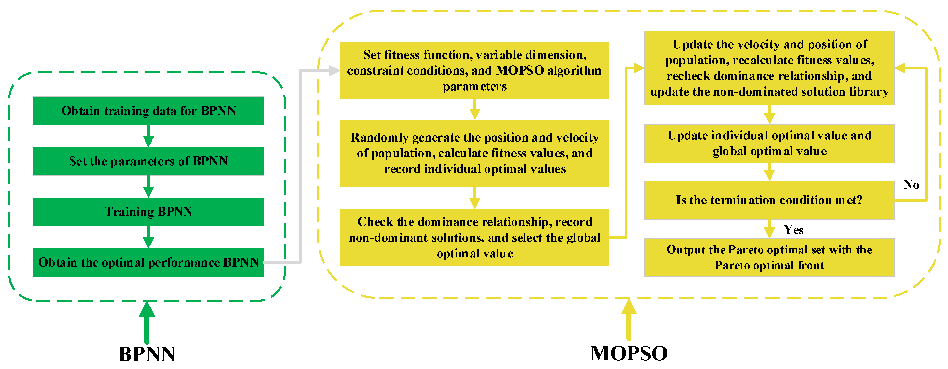
Figure 5.
Comparison of the optimal network performance under each number of hidden-layer neurons (R2, RMSE, and MAE denote the coefficient of determination, root mean square error, and mean absolute error between experimental and BPNN-predicted values, respectively; ¯ denotes average value of network performance indices for missing index and reseeding index; TR and TS denote training set and test set, respectively).
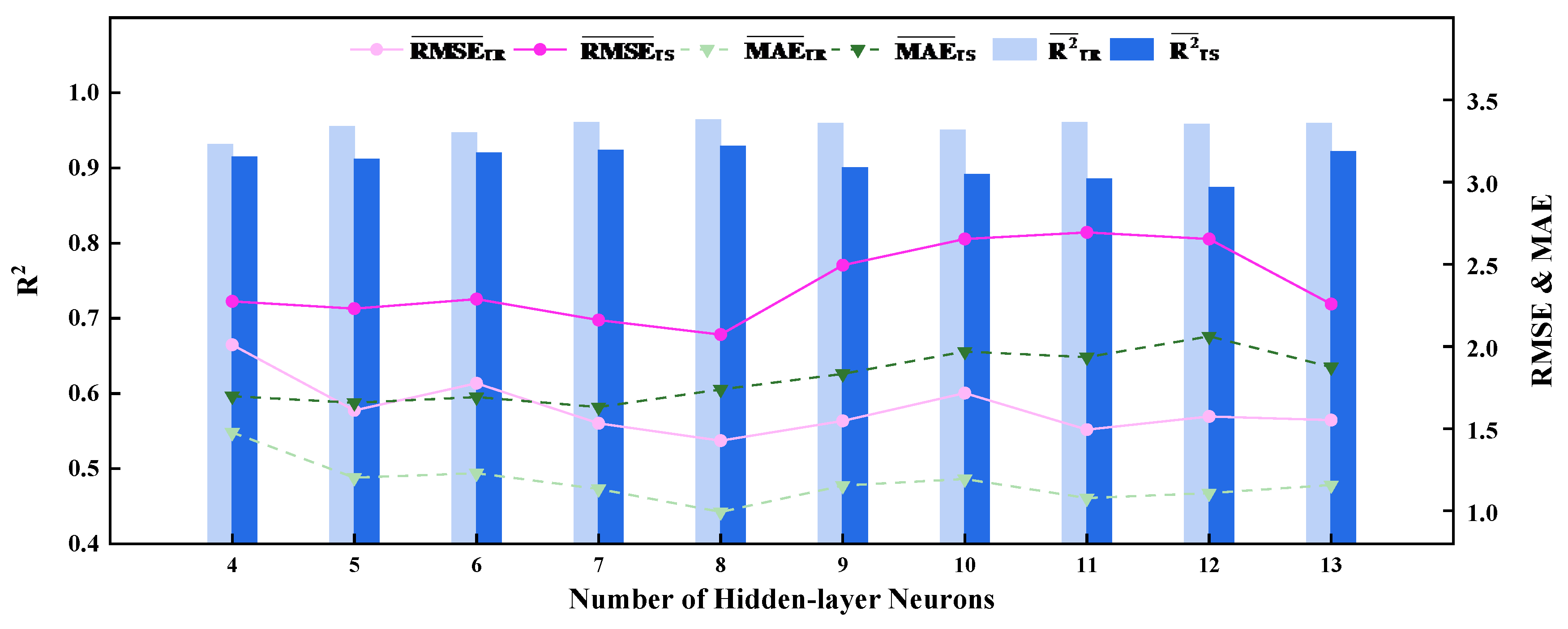
Figure 6.
Comparison of optimal network performance under each activation function combination (R2, RMSE, and MAE denote the coefficient of determination, root mean square error, and mean absolute error between experimental and BPNN-predicted values, respectively; ¯ denotes average value of network performance indices for missing index and reseeding index; TR and TS denote training set and test set, respectively).
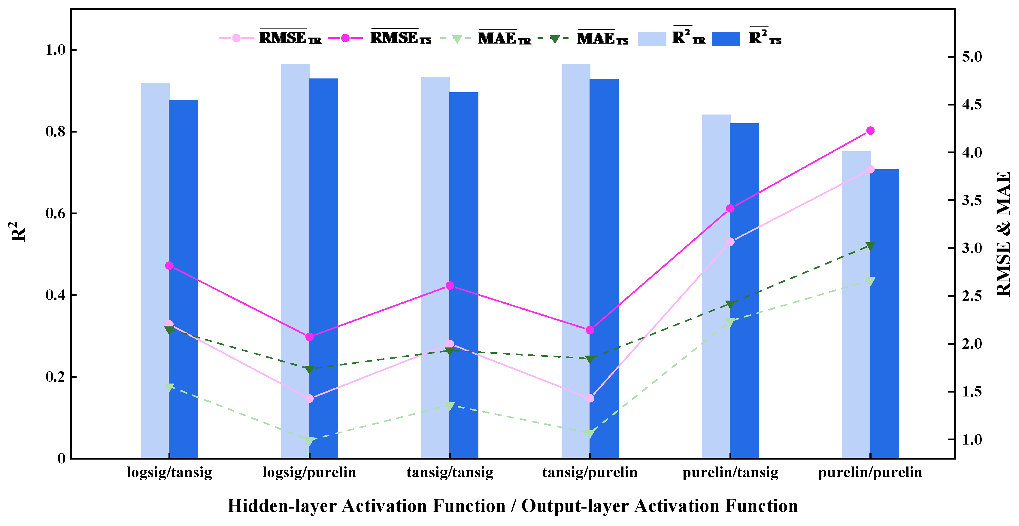
Figure 7.
Comparison of the experimental and BPNN-predicted values for the missing index (MI).
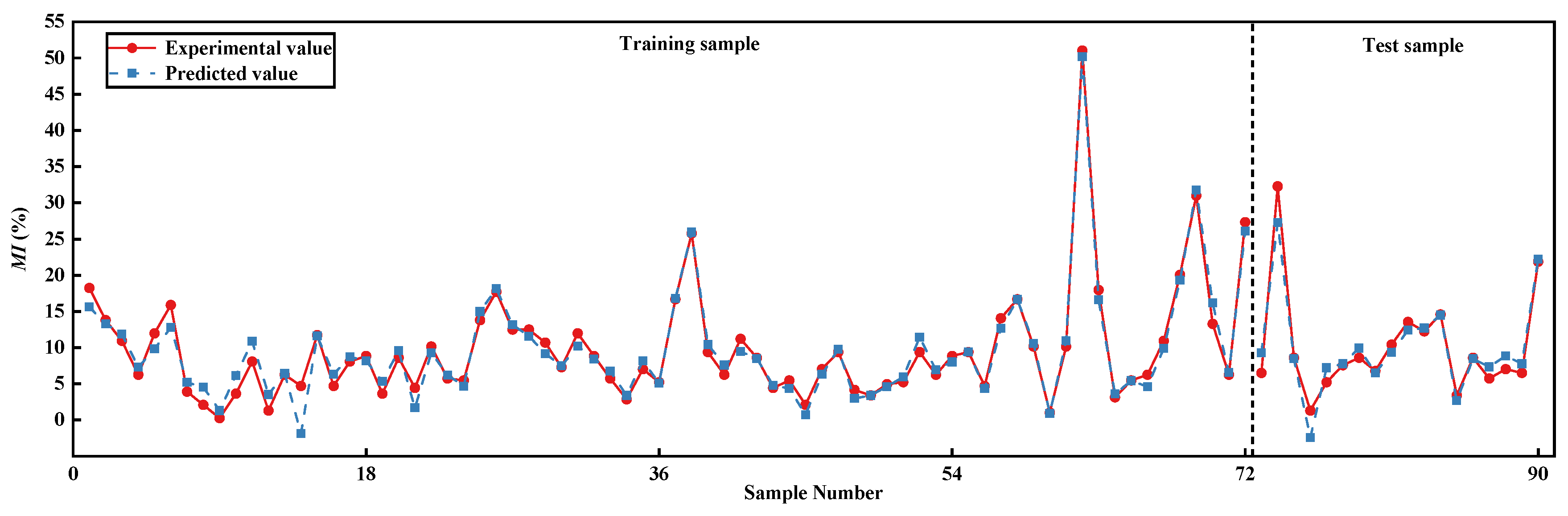
Figure 8.
Comparison of the experimental and BPNN-predicted values for the reseeding index (RI).
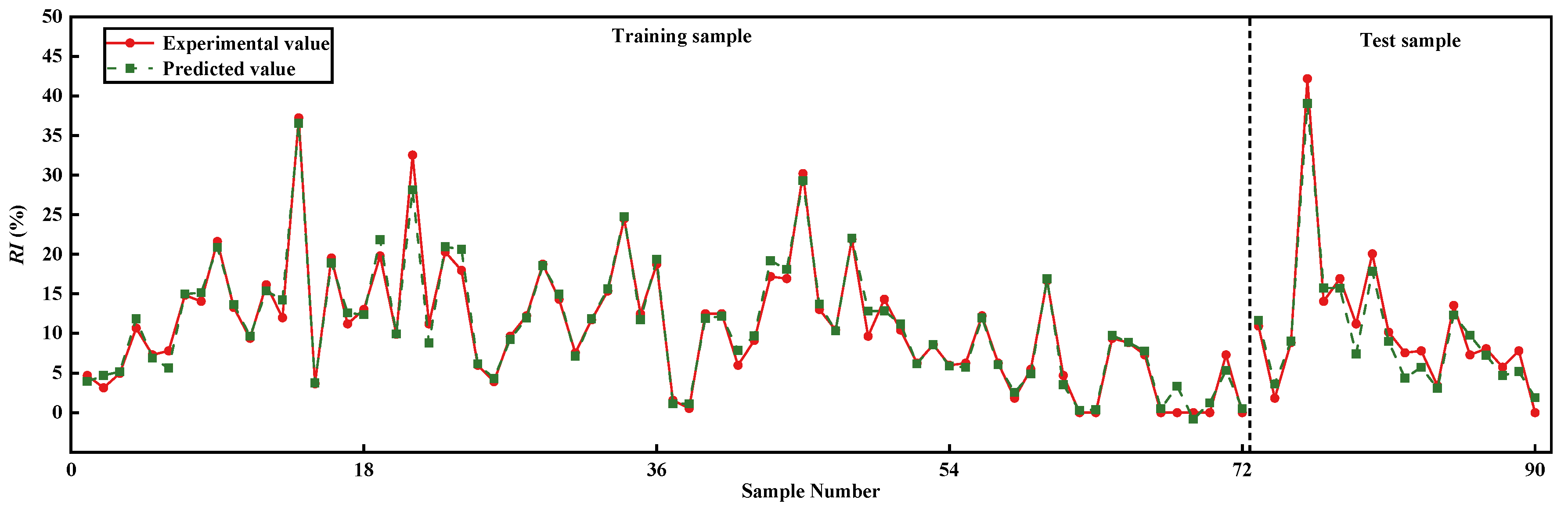
Figure 9.
Comparison of optimal experimental and optimized results (QI denotes qualified index).
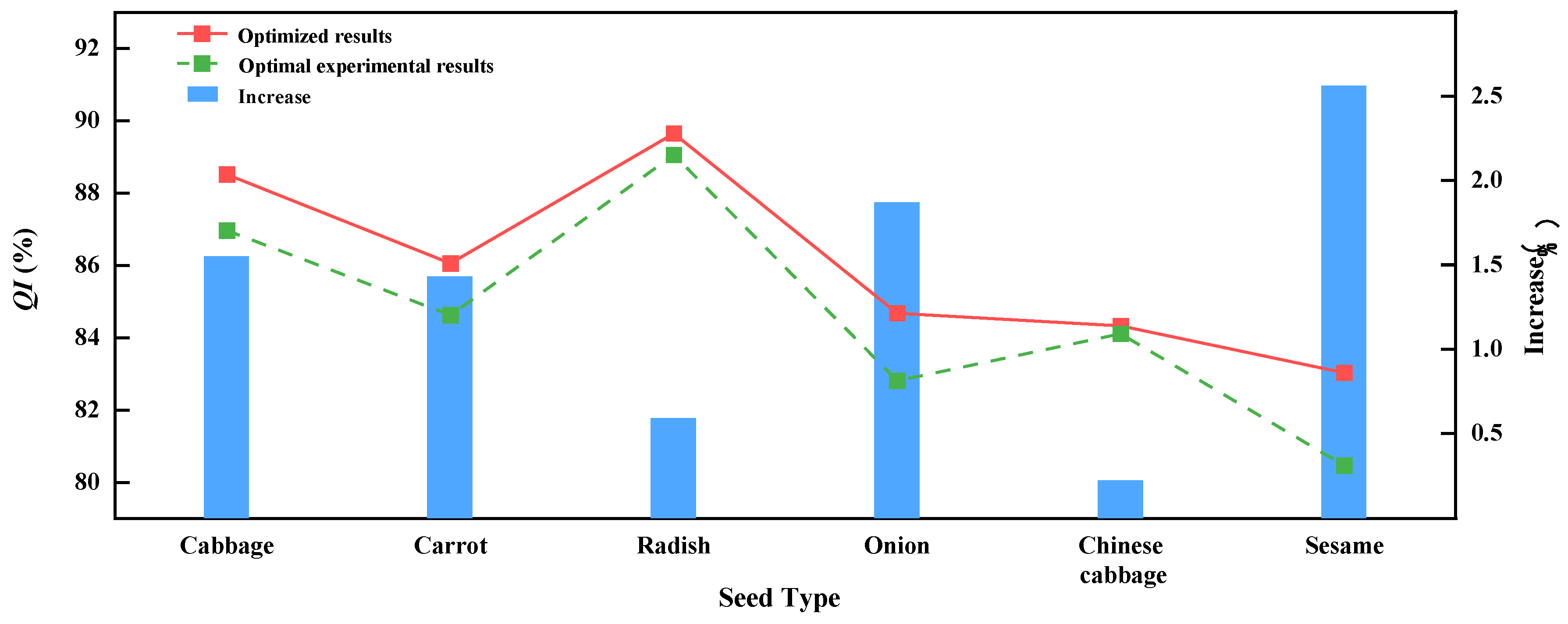
Figure 10.
Pareto optimal frontiers for (a) tomato; (b) pepper; and (c) Bok choi (RI and MI denote reseeding index and missing index, respectively).
Figure 10.
Pareto optimal frontiers for (a) tomato; (b) pepper; and (c) Bok choi (RI and MI denote reseeding index and missing index, respectively).
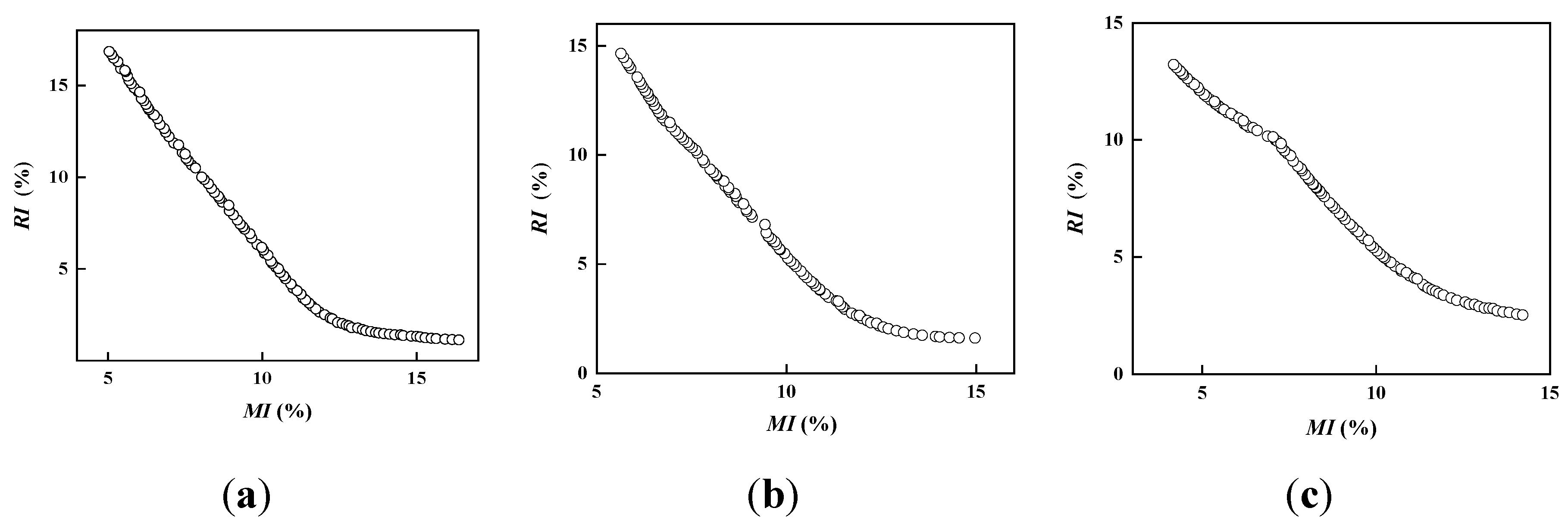

Table 1.
Range of influencing factors.
| Seed Type | Vacuum Pressure (kPa) | Rotational Speed (rpm) | Hole Diameter (mm) |
|---|---|---|---|
| Chinese cabbage | 6–10 | 10–14 | 0.6–1.0 |
| Carrot | |||
| Sesame | |||
| Onion | |||
| Cabbage | 8–12 | ||
| Radish | 10–14 |
Table 2.
Factor level settings.
| Factor | Level | ||
|---|---|---|---|
| 1 | 2 | 3 | |
| Hole diameter (mm) |
0.6 | 0.8 | 1.0 |
| Vacuum pressure (kPa) |
6/8/10 | 8/10/12 | 10/12/14 |
| Rotational speed (rpm) |
10 | 12 | 14 |
Table 3.
Orthogonal experiment results for Chinese cabbage seed.
| Seed Type | Hole Diameter (mm) |
Vacuum Pressure (kPa) |
Rotational Speed (rpm) |
Missing Index (%) |
Reseeding Index (%) |
Qualified Index (%) |
|---|---|---|---|---|---|---|
| Chinese cabbage | 0.6 | 6 | 10 | 18.23 | 4.69 | 77.08 |
| 6 | 14 | 32.29 | 1.82 | 65.89 | ||
| 8 | 12 | 13.80 | 3.13 | 83.07 | ||
| 10 | 14 | 10.94 | 4.95 | 84.11 | ||
| 10 | 10 | 6.51 | 10.94 | 82.55 | ||
| 0.8 | 8 | 10 | 6.25 | 10.68 | 83.07 | |
| 8 | 14 | 11.98 | 7.29 | 80.73 | ||
| 6 | 12 | 15.89 | 7.81 | 76.30 | ||
| 8 | 12 | 8.59 | 8.85 | 82.55 | ||
| 10 | 12 | 3.91 | 14.84 | 81.25 | ||
| 1.0 | 8 | 12 | 2.08 | 14.06 | 83.86 | |
| 10 | 10 | 0.26 | 21.61 | 78.13 | ||
| 6 | 10 | 3.65 | 13.28 | 83.07 | ||
| 6 | 14 | 8.07 | 9.38 | 82.55 | ||
| 10 | 14 | 1.30 | 16.15 | 82.55 |
Table 4.
Orthogonal experiment results for carrot seed.
| Seed Type | Hole Diameter (mm) |
Vacuum Pressure (kPa) |
Rotational Speed (rpm) |
Missing Index (%) |
Reseeding Index (%) |
Qualified Index (%) |
|---|---|---|---|---|---|---|
| Carrot | 0.6 | 6 | 10 | 8.59 | 9.89 | 81.52 |
| 6 | 14 | 11.72 | 3.65 | 84.63 | ||
| 8 | 12 | 8.07 | 11.20 | 80.73 | ||
| 10 | 14 | 7.55 | 16.93 | 75.52 | ||
| 10 | 10 | 5.73 | 20.31 | 73.96 | ||
| 0.8 | 8 | 10 | 4.69 | 19.53 | 75.78 | |
| 8 | 14 | 8.85 | 13.02 | 78.13 | ||
| 6 | 12 | 10.16 | 11.20 | 78.64 | ||
| 8 | 12 | 5.21 | 14.06 | 80.73 | ||
| 10 | 12 | 3.65 | 19.79 | 76.56 | ||
| 1.0 | 8 | 12 | 4.43 | 32.55 | 63.02 | |
| 10 | 10 | 1.30 | 42.19 | 56.51 | ||
| 6 | 10 | 5.47 | 17.97 | 76.56 | ||
| 6 | 14 | 6.25 | 11.98 | 81.77 | ||
| 10 | 14 | 4.69 | 37.24 | 58.07 |
Table 5.
Orthogonal experiment results for sesame seed.
| Seed Type | Hole Diameter (mm) |
Vacuum Pressure (kPa) |
Rotational Speed (rpm) |
Missing Index (%) |
Reseeding Index (%) |
Qualified Index (%) |
|---|---|---|---|---|---|---|
| Sesame | 0.6 | 6 | 10 | 13.80 | 5.99 | 80.21 |
| 6 | 14 | 17.71 | 3.91 | 78.39 | ||
| 8 | 12 | 12.50 | 9.64 | 77.86 | ||
| 10 | 14 | 12.50 | 12.24 | 75.26 | ||
| 10 | 10 | 10.68 | 18.75 | 70.57 | ||
| 0.8 | 8 | 10 | 7.29 | 14.32 | 78.39 | |
| 8 | 14 | 10.42 | 10.16 | 79.42 | ||
| 6 | 12 | 11.98 | 7.55 | 80.47 | ||
| 8 | 12 | 8.85 | 11.72 | 79.43 | ||
| 10 | 12 | 6.77 | 20.05 | 73.18 | ||
| 1.0 | 8 | 12 | 5.73 | 15.36 | 78.91 | |
| 10 | 10 | 2.86 | 24.48 | 72.66 | ||
| 6 | 10 | 7.03 | 12.50 | 80.47 | ||
| 6 | 14 | 8.59 | 11.20 | 80.21 | ||
| 10 | 14 | 5.21 | 18.75 | 76.04 |
Table 6.
Orthogonal experiment results for onion seed.
| Seed Type | Hole Diameter (mm) |
Vacuum Pressure (kPa) |
Rotational Speed (rpm) |
Missing Index (%) |
Reseeding Index (%) |
Qualified Index (%) |
|---|---|---|---|---|---|---|
| Onion | 0.6 | 6 | 10 | 16.67 | 1.56 | 81.77 |
| 6 | 14 | 25.78 | 0.52 | 73.70 | ||
| 8 | 12 | 14.58 | 3.39 | 82.03 | ||
| 10 | 14 | 12.24 | 7.81 | 79.95 | ||
| 10 | 10 | 9.38 | 12.50 | 78.13 | ||
| 0.8 | 8 | 10 | 6.25 | 12.50 | 81.25 | |
| 8 | 14 | 11.20 | 5.99 | 82.81 | ||
| 6 | 12 | 13.54 | 7.55 | 78.91 | ||
| 8 | 12 | 8.59 | 9.11 | 82.29 | ||
| 10 | 12 | 4.43 | 17.19 | 78.39 | ||
| 1.0 | 8 | 12 | 5.47 | 16.93 | 77.60 | |
| 10 | 10 | 2.08 | 30.21 | 67.71 | ||
| 6 | 10 | 7.03 | 13.02 | 79.95 | ||
| 6 | 14 | 9.38 | 10.42 | 80.21 | ||
| 10 | 14 | 4.17 | 21.88 | 73.96 |
Table 7.
Orthogonal experiment results for cabbage seed.
| Seed Type | Hole Diameter (mm) |
Vacuum Pressure (kPa) |
Rotational Speed (rpm) |
Missing Index (%) |
Reseeding Index (%) |
Qualified Index (%) |
|---|---|---|---|---|---|---|
| Cabbage | 0.6 | 12 | 14 | 10.16 | 5.47 | 84.37 |
| 10 | 12 | 9.38 | 6.25 | 84.37 | ||
| 8 | 10 | 14.06 | 6.25 | 79.69 | ||
| 8 | 14 | 16.67 | 1.82 | 81.51 | ||
| 12 | 10 | 8.59 | 7.29 | 84.12 | ||
| 0.8 | 10 | 10 | 5.21 | 10.42 | 84.37 | |
| 10 | 14 | 8.85 | 5.99 | 85.16 | ||
| 8 | 12 | 9.38 | 6.25 | 84.37 | ||
| 10 | 12 | 6.25 | 8.59 | 85.16 | ||
| 12 | 12 | 4.69 | 12.24 | 83.07 | ||
| 1.0 | 8 | 14 | 5.73 | 8.07 | 86.20 | |
| 8 | 10 | 4.95 | 14.32 | 80.73 | ||
| 10 | 12 | 3.39 | 9.64 | 86.97 | ||
| 12 | 14 | 3.39 | 13.54 | 83.07 | ||
| 12 | 10 | 1.04 | 16.67 | 82.29 |
Table 8.
Orthogonal experiment results for radish seed.
| Seed Type | Hole Diameter (mm) |
Vacuum Pressure (kPa) |
Rotational Speed (rpm) |
Missing Index (%) |
Reseeding Index (%) |
Qualified Index (%) |
|---|---|---|---|---|---|---|
| Radish | 0.6 | 12 | 12 | 27.34 | 0.00 | 72.66 |
| 10 | 14 | 51.04 | 0.00 | 48.96 | ||
| 10 | 10 | 30.99 | 0.00 | 69.01 | ||
| 14 | 10 | 20.05 | 0.00 | 79.95 | ||
| 14 | 14 | 21.88 | 0.00 | 78.12 | ||
| 0.8 | 12 | 10 | 6.51 | 7.81 | 85.68 | |
| 12 | 14 | 10.16 | 4.69 | 85.15 | ||
| 10 | 12 | 13.28 | 0.00 | 86.72 | ||
| 12 | 12 | 7.03 | 5.73 | 87.24 | ||
| 14 | 12 | 5.47 | 8.85 | 85.68 | ||
| 1.0 | 14 | 14 | 6.25 | 7.29 | 86.46 | |
| 14 | 10 | 3.13 | 9.38 | 87.49 | ||
| 12 | 12 | 6.25 | 7.29 | 86.46 | ||
| 10 | 10 | 10.94 | 0.00 | 89.06 | ||
| 10 | 14 | 17.97 | 0.00 | 82.03 |
Table 12.
Settings of the MOPSO algorithm parameters.
| Parameter | Value |
|---|---|
| Population size | 100 |
| Non-dominated solution library size | 100 |
| No. of iterations | 200 |
| Individual learning coefficient | 1.5 |
| Global learning coefficient | 1.5 |
| Number of grids per dimension | 40 |
| Inertia weight | Max: 0.9 |
| Min: 0.4 |
Table 9.
Physical properties of seed types.
| Seed Type | Geometric Mean Diameter (mm) |
Sphericity (%) |
Thousand-Grain Weight (g) |
Kernel Density (g·cm-3) |
|---|---|---|---|---|
| Chinese cabbage | 1.73±0.11 | 89.27±2.96 | 3.13±0.10 | 0.977±0.026 |
| Carrot | 1.56±0.17 | 46.10±5.19 | 1.84±0.07 | 1.155±0.016 |
| Sesame | 1.71±0.10 | 55.34±2.43 | 3.06±0.07 | 0.930±0.027 |
| Onion | 2.04±0.11 | 68.99±4.69 | 3.28±0.02 | 1.131±0.014 |
| Cabbage | 1.75±0.13 | 86.25±5.73 | 3.64±0.16 | 0.940±0.021 |
| Radish | 2.62±0.19 | 76.25±3.64 | 11.27±0.44 | 1.042±0.014 |
Table 10.
Test set data.
| No. | Geometric Mean Diameter (mm) |
Sphericity (%) |
Thousand-Grain Weight (g) |
Kernel Density (g·cm-3) |
Hole Diameter (mm) |
Vacuum Pressure (kPa) | Rotational Speed (rpm) | Missing Index (%) |
Reseeding Index (%) |
|---|---|---|---|---|---|---|---|---|---|
| 1 | 1.73 | 89.27 | 3.13 | 0.977 | 0.6 | 10 | 10 | 6.51 | 10.94 |
| 2 | 1.73 | 89.27 | 3.13 | 0.977 | 0.6 | 6 | 14 | 32.29 | 1.82 |
| 3 | 1.73 | 89.27 | 3.13 | 0.977 | 0.8 | 8 | 12 | 8.59 | 8.85 |
| 4 | 1.56 | 46.10 | 1.84 | 1.155 | 1.0 | 10 | 10 | 1.30 | 42.19 |
| 5 | 1.56 | 46.10 | 1.84 | 1.155 | 0.8 | 8 | 12 | 5.21 | 14.06 |
| 6 | 1.56 | 46.10 | 1.84 | 1.155 | 0.6 | 10 | 14 | 7.55 | 16.93 |
| 7 | 1.71 | 55.34 | 3.06 | 0.930 | 1.0 | 6 | 14 | 8.59 | 11.20 |
| 8 | 1.71 | 55.34 | 3.06 | 0.930 | 0.8 | 10 | 12 | 6.77 | 20.05 |
| 9 | 1.71 | 55.34 | 3.06 | 0.930 | 0.8 | 8 | 14 | 10.42 | 10.16 |
| 10 | 2.04 | 68.99 | 3.28 | 1.131 | 0.8 | 6 | 12 | 13.54 | 7.55 |
| 11 | 2.04 | 68.99 | 3.28 | 1.131 | 0.6 | 10 | 14 | 12.24 | 7.81 |
| 12 | 2.04 | 68.99 | 3.28 | 1.131 | 0.6 | 8 | 12 | 14.58 | 3.39 |
| 13 | 1.75 | 86.25 | 3.64 | 0.940 | 1.0 | 12 | 14 | 3.39 | 13.54 |
| 14 | 1.75 | 86.25 | 3.64 | 0.940 | 0.6 | 12 | 10 | 8.59 | 7.29 |
| 15 | 1.75 | 86.25 | 3.64 | 0.940 | 1.0 | 8 | 14 | 5.73 | 8.07 |
| 16 | 2.62 | 76.25 | 11.27 | 1.042 | 0.8 | 12 | 12 | 7.03 | 5.73 |
| 17 | 2.62 | 76.25 | 11.27 | 1.042 | 0.8 | 12 | 10 | 6.51 | 7.81 |
| 18 | 2.62 | 76.25 | 11.27 | 1.042 | 0.6 | 14 | 14 | 21.88 | 0.00 |
Table 11.
Settings of the BPNN training parameters.
| Parameter | Value |
|---|---|
| Maximum no. of iterations | 1000 |
| Target error | 1×10⁻⁴ |
| Learning rate | 0.01 |
| Training algorithm | Levenberg-Marquardt |
Table 13.
Values of e, f, g, and h for each seed.
| Seed Type | x2 | x3 | ||
|---|---|---|---|---|
| e | f | g | h | |
| Cabbage | 8 | 12 | 10 | 18 |
| Carrot | 4 | 8 | 14 | |
| Radish | 10 | 16 | ||
| Tomato | 4 | 10 | ||
| Chinese cabbage | 6 | |||
| Sesame | ||||
| Onion | ||||
| Bok choi | ||||
| Pepper | 18 | |||
Table 14.
Optimal network performance under each number of hidden-layer neurons (R2, RMSE, and MAE denote the coefficient of determination, root mean square error, and mean absolute error between experimental and BPNN-predicted values, respectively; ¯ denotes average value of network performance indices for missing index and reseeding index).
| No. of Hidden-layer Neurons |
Average Value of Network Performance Indices for Two Outputs | |||||
|---|---|---|---|---|---|---|
| Performance Indices for the Training Set | Performance Indices for the Test Set | |||||
| 4 | 2.0104 | 1.4775 | 0.9313 | 2.2744 | 1.6981 | 0.9141 |
| 5 | 1.6113 | 1.2020 | 0.9549 | 2.2306 | 1.6582 | 0.9112 |
| 6 | 1.7768 | 1.2297 | 0.9466 | 2.2881 | 1.6919 | 0.9196 |
| 7 | 1.5325 | 1.1333 | 0.9601 | 2.1607 | 1.6319 | 0.9231 |
| 8 | 1.4273 | 0.9935 | 0.9641 | 2.0728 | 1.7391 | 0.9290 |
| 9 | 1.5477 | 1.1539 | 0.9593 | 2.4943 | 1.8335 | 0.9004 |
| 10 | 1.7167 | 1.1945 | 0.9500 | 2.6538 | 1.9693 | 0.8913 |
| 11 | 1.4944 | 1.0783 | 0.9602 | 2.6942 | 1.9353 | 0.8850 |
| 12 | 1.5744 | 1.1079 | 0.9579 | 2.6539 | 2.0620 | 0.8738 |
| 13 | 1.5520 | 1.1576 | 0.9591 | 2.2583 | 1.8748 | 0.9218 |
Table 15.
Optimal network performance under each activation function combination (R2, RMSE, and MAE denote the coefficient of determination, root mean square error, and mean absolute error between experimental and BPNN-predicted values, respectively; ¯ denotes average value of network performance indices for missing index and reseeding index).
| Hidden-Layer Activation Function |
Output-Layer Activation Function |
Average Value of Network Performance Indices for Two Outputs | |||||
|---|---|---|---|---|---|---|---|
| Performance Indices for the Training Set | Performance Indices for the Test Set | ||||||
| Logsig | Tansig | 2.2038 | 1.5565 | 0.9179 | 2.8172 | 2.1504 | 0.8766 |
| Logsig | Purelin | 1.4273 | 0.9935 | 0.9641 | 2.0728 | 1.7391 | 0.9290 |
| Tansig | Tansig | 2.0002 | 1.3602 | 0.9323 | 2.6083 | 1.9306 | 0.8949 |
| Tansig | Purelin | 1.4303 | 1.0685 | 0.9646 | 2.1444 | 1.8452 | 0.9281 |
| Purelin | Tansig | 3.0668 | 2.2387 | 0.8409 | 3.4141 | 2.4209 | 0.8192 |
| Purelin | Purelin | 3.8248 | 2.6658 | 0.7512 | 4.2289 | 3.0312 | 0.7071 |
Table 16.
Performance of the optimal performance network (R2, RMSE, and MAE denote the coefficient of determination, root mean square error, and mean absolute error between experimental and BPNN-predicted values, respectively).
Table 16.
Performance of the optimal performance network (R2, RMSE, and MAE denote the coefficient of determination, root mean square error, and mean absolute error between experimental and BPNN-predicted values, respectively).
| Network | Output | Dataset | Performance Indices | ||
|---|---|---|---|---|---|
| BPNN (7-8-2) |
Missing index | Training set | 1.4883 | 1.0937 | 0.9627 |
| Test set | 1.8807 | 1.3440 | 0.9287 | ||
| Reseeding index | Training set | 1.2064 | 0.8436 | 0.9753 | |
| Test set | 2.0178 | 1.7559 | 0.9497 | ||
Table 17.
Weights and biases of the optimal performance BPNN.
| Connection Weight Between Input and Hidden Layers W1 |
Connection Weight between Hidden and Output Layers (Transposition) W2T |
Hidden-layer Bias bh |
Output- layer Bias bo |
|||||||
|---|---|---|---|---|---|---|---|---|---|---|
| −2.7320 | −1.3529 | −0.6447 | 0.5044 | 0.7261 | 3.9120 | −0.9372 | −2.1289 | −0.5536 | 6.0500 | 3.1567 |
| 2.2852 | 2.0053 | −1.2572 | 0.5124 | 3.9060 | 0.9832 | 0.1191 | 0.5815 | −1.7001 | −4.0843 | −2.1084 |
| −2.3290 | 0.2466 | 0.3522 | 0.8968 | 4.4255 | 0.5757 | −0.0804 | −1.4565 | 0.3460 | 6.4274 | |
| −1.6748 | −0.3326 | 0.8352 | 0.3386 | 0.3735 | 2.1485 | −0.5065 | −0.2870 | 1.3906 | 0.0285 | |
| 0.4245 | 0.2209 | 4.0421 | −0.1324 | −0.7695 | −2.7666 | −1.7444 | 0.0490 | −0.2990 | −3.8582 | |
| −0.1538 | −1.4328 | 1.3190 | −2.7081 | −0.5418 | −1.2597 | −0.6917 | −0.0582 | 0.2649 | −0.5468 | |
| 0.5534 | 1.7438 | −0.7404 | 1.0796 | 2.8059 | 1.2724 | 0.0536 | −0.8076 | 2.3069 | −2.5635 | |
| 1.8411 | −1.7465 | −3.2982 | 2.4162 | −0.7691 | −1.9419 | 0.2147 | −0.0975 | 1.2290 | 3.1703 | |
Table 18.
Comparison of the optimal experimental and optimized results.
| Seed Type | Optimal Result |
Parameter | Indices | ||||
|---|---|---|---|---|---|---|---|
| Hole Diameter (mm) |
Vacuum Pressure (kPa) |
Rotational Speed (rpm) |
Missing Index (%) |
Reseeding Index (%) |
Qualified Index (%) |
||
| Cabbage | Experiment | 1.00 | 10.0 | 12 | 3.39 | 9.64 | 86.97 |
| Optimization | 1.00 | 11.6 | 18 | 5.20 | 6.28 | 88.52 | |
| Carrot | Experiment | 0.60 | 6.0 | 14 | 11.72 | 3.65 | 84.63 |
| Optimization | 0.77 | 4.3 | 14 | 11.70 | 2.24 | 86.06 | |
| Radish | Experiment | 1.00 | 10.0 | 10 | 10.94 | 0.00 | 89.06 |
| Optimization | 0.98 | 10.6 | 10 | 8.76 | 1.59 | 89.65 | |
| Onion | Experiment | 0.80 | 8.0 | 14 | 11.20 | 5.99 | 82.81 |
| Optimization | 0.71 | 6.2 | 10 | 11.96 | 3.36 | 84.68 | |
| Chinese cabbage | Experiment | 0.60 | 10.0 | 14 | 10.94 | 4.95 | 84.11 |
| Optimization | 0.70 | 9.0 | 14 | 10.48 | 5.19 | 84.33 | |
| Sesame | Experiment | 1.00 | 6.0 | 10 | 7.03 | 12.50 | 80.47 |
| Optimization | 0.85 | 6.3 | 14 | 10.52 | 6.46 | 83.03 | |
Table 19.
Physical properties of three types of seeds.
| Seed Type | Geometric Mean Diameter (mm) |
Sphericity (%) |
Thousand-Grain Weight (g) |
Kernel Density (g·cm-3) |
|---|---|---|---|---|
| Tomato | 1.78±0.13 | 52.33±4.17 | 3.02±0.06 | 1.147±0.058 |
| Pepper | 2.19±0.21 | 54.60±3.77 | 5.47±0.05 | 0.937±0.054 |
| Bok choi | 1.60±0.10 | 93.14±2.79 | 2.60±0.05 | 0.975±0.039 |
Table 20.
Optimization results.
| Seed Type | Parameter | Indices | ||||
|---|---|---|---|---|---|---|
| Hole Diameter (mm) | Vacuum Pressure (kPa) |
Rotational Speed (rpm) |
Missing Index (%) |
Reseeding Index (%) |
Qualified Index (%) |
|
| Tomato | 0.75 | 5.6 | 13.7 | 11.85 | 2.66 | 85.50 |
| Pepper | 1.00 | 10.4 | 18.0 | 11.54 | 2.94 | 85.52 |
| Bok choi | 0.67 | 8.6 | 14.0 | 10.72 | 4.41 | 84.87 |
Table 21.
Verification results.
| Seed Type | Missing Index (%) |
Reseeding Index (%) |
Qualified Index (%) |
|
|---|---|---|---|---|
| Tomato | Predicted value | 11.85 | 2.66 | 85.50 |
| Experimental value | 11.19 | 2.08 | 86.73 | |
| Absolute error | 0.66 | 0.58 | 1.23 | |
| Pepper | Predicted value | 11.54 | 2.94 | 85.52 |
| Experimental value | 8.85 | 3.65 | 87.50 | |
| Absolute error | 2.69 | 0.71 | 1.98 | |
| Bok choi | Predicted value | 10.72 | 4.41 | 84.87 |
| Experimental value | 9.11 | 5.21 | 85.68 | |
| Absolute error | 1.61 | 0.80 | 0.81 |
Disclaimer/Publisher’s Note: The statements, opinions and data contained in all publications are solely those of the individual author(s) and contributor(s) and not of MDPI and/or the editor(s). MDPI and/or the editor(s) disclaim responsibility for any injury to people or property resulting from any ideas, methods, instructions or products referred to in the content. |
© 2025 by the authors. Licensee MDPI, Basel, Switzerland. This article is an open access article distributed under the terms and conditions of the Creative Commons Attribution (CC BY) license (http://creativecommons.org/licenses/by/4.0/).
Copyright: This open access article is published under a Creative Commons CC BY 4.0 license, which permit the free download, distribution, and reuse, provided that the author and preprint are cited in any reuse.


