
Submitted:
26 January 2025
Posted:
27 January 2025
You are already at the latest version
Abstract
As the global energy landscape evolves towards sustainability, the extensive usage of fossil fuels in electricity generation is progressively diminishing, while the contribution of renewable energy sources is steadily increasing. In this evolving scenario,importance of load forecasting cannot be overstated in optimising energy management and ensuring the efficient operation of industrial plants regardless of their scale. By accurately anticipating energy demand, industral facilities can enhance efficiency, reduce costs, and facilitate the adoption of renewable energy technologies in the power grid. Recent studies have emphasised the pervasive utilisation of machine learning-based algorithms in the field of electric load forecasting for industrial plants. Their capacity to analyse intricate patterns and enhance prediction accuracy renders them a favoured option for enhancing energy management and operational efficiency. The present analysis revolves around the creation of short-term electric load forecasting models for a large industrial plant operating in Adana, Türkiye. The integration of calendar, meteorological, and lagging electrical variables, along with machine learning-based algorithms, is employed to boost forecasting accuracy and optimize energy utilization.The ultimate objective of the present study is to conduct a thoroughgoing and detailed analysis of statistical performance and associated error metrics. The metrics to be employed include the R², MAE, RMSE, and MAPE.
Keywords:
Multiple Linear Regression (MLR)
; Group Method of Data Handling (GMDH)
; MultiLayer Perceptron Neural Netwok (MLPNN)
; Gradient Boost Decision Tree (GBDT)
; Gene Expression Programming (GEP)
1. Introduction
In recent years, several critical factors have converged to position the forecasting of electrical energy consumption as an essential task. These factors include not only the significant increase in electrical energy consumption within industrial plants, but also its direct impact on production costs, the growing necessity for uninterrupted energy supply, and the specific changes occurring within power systems. This task assumes particular significance for large industrial plants, as it exerts a direct influence on operational efficiency, cost management, and long-term energy planning. Precisely forecasting electrical energy consumption is therefore a pivotal element in ensuring sustainability and profitability [1]. In the contexts of industrial plants, the necessity for highly precise energy forecasting models has become progressively imperative. These models have been shown to act as a cornerstone for ensuring the efficient use and management of energy resources, facilitating the planning and scheduling of maintenance activities, and providing a clear understanding of how energy consumption directly affects product costs. The utilisation of sophisticated forecasting methodologies empowers industrial plants to enhance operational efficiency, mitigate energy wastage, optimise long-term energy strategies, enhance cost-effectiveness, align energy utilisation with production objectives, and consequently augment sustainability and profitability [2]. Energy consumption is influenced by a variety of factors, with each factor contributing to variations in demand. Social and economic dynamics, including changes in population, industrial activity, and consumer behaviour, have been shown to have a significant impact on energy needs. Furthermore, seasonal factors are also of crucial importance, as energy consumption often exhibits a distinct increase during certain periods, such as in winter for heating or summer for cooling. Moreover, climatic conditions, including temperature, humidity, and weather patterns, directly influence energy demand, particularly in regions with extreme weather conditions. The intricate nature of these interactions necessitates the development of sophisticated forecasting methodologies that account for the combined effects of these factors to ensure the optimisation of energy management strategies [3]. This investigation aims mainly to predict the electrical load of an industrial plant located in Adana, Turkey. In this context, five different methodologies are applied: MLR, a traditional linear model, and GMDH, a machine learning-based approach. Additionally, MLPNN, GBDT, and GEP are utilised. The performance and accuracy of these methods are then assessed in order to determine their effectiveness in forecasting energy consumption at the facility.The field of load forecasting can be categorised into four distinct types, as determined by the length of the prediction time interval. Figure 1 illustrates the categorization according to their respective forecasting time.
Each category has specific uses that support different operational, planning, and strategic decision-making processes in energy management.The initial category is long-term forecasting, which refers to the prediction of electric load for extended periods, typically ranging from three years to 50 years. This type of forecasting is useful for strategic planning and infrastructure development. Medium-term forecasting, on the other hand, is employed when the time frame extends from two weeks to three years, providing valuable insights for effective resource allocation and budgeting by energy suppliers. The third category is that of short-term electric load forecasting (STLF), which focuses on predicting electricity demand for shorter time frames, such as hours, days or weeks. This type of forecasting is particularly important for operational management and optimising energy generation. Very short-term forecasting, on the other account, focuses on predicting electric loads for even shorter time frames, typically from a few minutes to an hour, and is crucial for real-time decision-making, such as grid balancing and load dispatch [3,4,5,6,7,8]. Methods performed using electric load forecasting are shown in Table 1.
Since energy consumption forecasting is critical to the planning, financing, maintenance and operational management of industrial facilities, several advanced statistical and machine learning-based methods are being developed and implemented to improve the accuracy and efficiency of these processes. These methods help to optimise resource allocation, reduce operating costs and improve overall system reliability by providing more accurate and data-driven predictions. Recently, statistical techniques such as time series analysis and regression have received considerable attention in the literature and have found wide application in predictive modelling and data analysis. Despite the efficacy of statistical techniques in addressing electric load forecasting, fluctuations in economic, sociological, and climatic factors have the potential to compromise the accuracy of forecasts, resulting in elevated error rates in prediction models. Machine learning-based methods are vital in the minimisation of errors and the enhancement of the accuracy of predictions. The effective identification of patterns in the fluctuations of electrical loads facilitates the utilisation of multiple variables as inputs, thereby ensuring the acquisition of highly dependable and accurate forecasting results. It is noteworthy that inputs which demonstrate minimal influence on the resulting prediction can have a negative impact on several key areas. Firstly, the accuracy of the final result can be diminished. Secondly, the complexity of the model can be increased. Thirdly, the time taken for computation can be prolonged.
2. Related Work
The literature has very different perspective studies which tried to explain energy consumption forecasting methodologies. In an effort to resolve these challenges and identify the predominant inputs in electrical load forecasting, the GMDH is widely utilized in various forms across the literature [9]. Ahmad et al. investigated the potential of applying a hybrid method that combines the Group Method of GMDH and LSSVM to predict electricity consumption in buildings [10]. In another study, Jinlian et al. proposed an approach that integrates GMDH networks, PSO, and LSSVM for electric load forecasting [11]. In relation to wind and solar-based renewable energy, Heydari et al. contributed to the development of a new algorithm that combines GMDH networks with a modified Fruit Fly Optimization Algorithm to predict energy production [12]. As previously stated, numerous factors influence the electrical load; therefore, high reliability must be ensured by the method used for its prediction. While certain factors, such as meteorological conditions and calendar data, are used as explanatory variables that provide broader context, they are not directly influential on the forecasted value. Conversely, other factors that directly influence electrical load forecasting exist and play a significant role in determining the accuracy of predictions. One of the statistical methods that is frequently employed for accurate electric load forecasting is the Multiple Linear Regression (MLR) method. The objective of utilising MLR is to model the relationship between the explanatory variables and the dependent variables as a linear function, thereby enabling precise predictions of the value to be calculated. The multiple linear regression method is frequently utilised in the existing literature for the purpose of electric load forecasting, due to the fact that it is a simple and user-friendly technique that can be executed more quickly than other techniques. These advantages make it a popular choice for modelling and predicting electrical load with a high degree of accuracy [13]. Sarduy et al. applied the multiple linear regression method in both linear and non-linear models to determine the highest load demand at the University of Sao Paulo [14]. Goia and Gustavsen utilized linear regression to assess the performance evaluation of a semi-integrated photovoltaic system in a zero-emission building[15]. In another study, Yükseltan et al. developed a method for hourly load forecasting in Turkey for annual, weekly, and daily periods by means of a linear model [16]. Similarly, Pino-Mejias et al. created linear regression models and artificial neural networks to forecast electrical load consumption in office buildings in Chile and compared the performance of these methods [17]. Additionally, numerous studies in the literature focus on electric load forecasting for healthcare facilities using linear regression models [18,19,20]. A number of studies have been conducted using GEP, an alternative forecasting method for electrical energy consumption. In their comparative analysis, Hosseini and Gandomi examined the application of GEP models in conjunction with MLSR and GRNN for the purpose of forecasting the day-ahead peak and total loads of a North American electric utility [21]. In their combination-based study, Fan and Zhu. found that the combination of EMD and GEP yielded results that were more accurate in comparison to other combinations that formed WD and GEP [22]. In a comparative study, Huo et al. evaluated the newly developed GEP model for load forecasting by contrasting it with traditional GP and GEP models [23]. Bakare et al. developed a hybrid method by combining the high flexibility and accuracy of the GEP algorithm and the ANFIS technique [24]. Tabatabaei et al., and Jalal et al., emphasized the GEP’s dominance over alternative AI models and expressed its potential for various applications [25,26] On the other hand, different studies were conducted by means of MLPNN. A hybrid load forecasting model is proposed that combines statistical methods and MLP to simultaneously provide short-, medium- and long-term forecasting results using medium quality data required for field applications. This hybrid model is proposed to decrease the problems of average convergence and to provide short to long term load predicting results [27]. To solve the MTLF (Mid-Term Load Forecasting) problem, MLP neural networks and optimization techniques were mixed [28]. A data-driven short-term load forecasting method has been proposed to predict electrical loads over time using features that reflect the non-linear and dynamic characteristics of loads. This method integrates advanced analytical techniques to improve prediction accuracy and adaptability to changing load patterns [29]. The proposed method uses a cumulative generalisation approach to manage stochastic fluctuations in load demand, allowing the model to progressively adapt to variations in historical data. By incorporating this approach, the method improves its ability to capture complex, dynamic load patterns while minimising the impact of random fluctuations. This results in more accurate and reliable short-term load forecasts, making the model more suitable for real-world applications where load demand is subject to unpredictable changes. XGB, LGBM, and MLP were formed this model [30]. On the other hand, the MLP method has been used in various studies in the literature for load forecasting in healthcare sector campuses [31,32].
3. Material and Methods
In the context of the study, the present section is entitled "Materials and Methods". The material employed in this research consists of the dataset, which serves as the foundation for analysis. Conversely, the methods encompass a range of forecasting techniques, which are designed to formulate model equations for the purpose of predictive analysis. The employment of these methods is intended to enhance the accuracy and reliability of predictions by utilising diverse statistical and machine learning-based approaches.
3.1. Material
The material for this study consists of the dataset, which undergoes a series of steps to ensure its suitability for analysis. Initially, the data is acquired from the relevant sources, after which it is cleaned and preprocessed to remove any inconsistencies or missing values. The dataset is then organised into three primary categories: electrical data, meteorological data, and calendar data. The categories are carefully structured to ensure compatibility and accuracy for subsequent analysis. Each of these data types is then subjected to further processing to extract meaningful features that are essential for the forecasting tasks. The detailed steps of this preparation process are outlined as follows.
3.1.1. Data Source and Acquisition
This study was conducted at an industrial facility capable of uninterrupted, 24/7 production. Given that the plant incorporates a variety of chemical processes during the production phase, the continuity of energy and accurate forecasting of energy consumption are of critical importance. The transformer installed at the facility had an installed capacity of 200 MVA. The subsequent data acquisition stage covers the period from 01/01/2020 to 31/12/2022 and is obtained from two transformers with a capacity of 100 MVA each, with a resolution of one hour. The electrical data utilised in the present study was obtained from the plant’s Energy SCADA System. Meteorological data were taken from MERRA-2 , a globally accessible database of meteorological variables managed by NASA.
3.1.2. Properties of Dataset
The dataset utilised for the purpose of electricity consumption estimation in this study is comprised of three input categories and 15 input variables, the details of which are provided in Table 2.
The input variables of the dataset are divided into three primary categories: electrical, meteorological, and calendar. The electrical variables represent the historical electrical energy consumed as recorded by the SCADA system, providing insight into past energy consumption patterns. The meteorological variables are derived from MERRA-2, which provides data on weather conditions Like temperature, humidity, and wind velocity, which can have an impact on energy consumption. Finally, the calendar variables include information on time-related factors, such as the day of the week, public holidays and the seasons of the year, which can also have an impact on energy consumption patterns. Furthermore, the calendar variables incorporated within the dataset encompass the hour of the day (0–23), the day of the month (1–31), the classification of the day (0 for working days and 1 for weekends and public holidays), the week of the year (1–53), and the month of the year (1–12), respectively. It is crucial to emphasise that these variables, which are based on time, facilitate a comprehensive understanding of the variation in energy consumption patterns across various times and dates.Basic flowchart of the system is depicted in the Figure 2.
3.2. Methods of Forecasting
The details of the MLR, GMDH, GBDT, MLPNN, and GEP methods employed in the study are thoroughly explained in the subsections of this section.
3.2.1. Multiple Linear Regression
In order to model the relationship between different explanatory variables, like weather and calendar information, and dependent variables that directly affect the amount of electric energy consumption in its linear form, the MLR, a statistical technique, is used in the forecasting of electric energy consumption.The method being used aims to reduce the difference between the estimated and real energy usage as much as feasible. [33]. A model based on the multiple linear regression method is formulated as follows:
In the above formula, y represents the amount of consumed electrical energy, stands for the independent variable, represents the regression parameter according to the independent variable and, lastly used for the error in the forecasting [34]. The most important reasons for the use of statistical MLR are its simplicity in terms of comprehension, ease of application and superior operational speed compared to alternative methods. Strengths and limitations of MLR is described in the Table 3.
3.2.2. Group Method of Data Handling
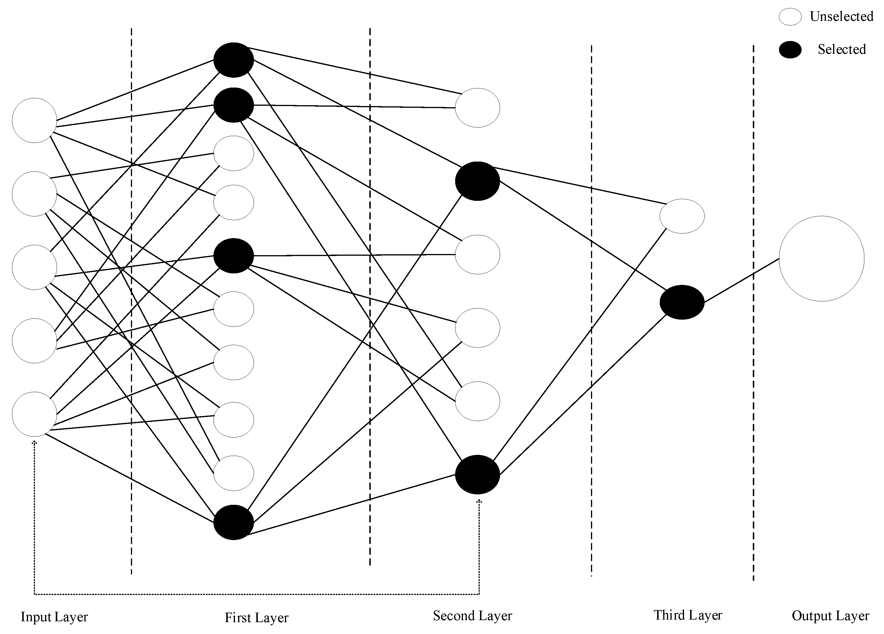
Neuron connections, the number of chosen neurons, network layers, and hidden layer neurons are all not preset in GMDH networks, which function as self-organizing systems. Rather, these structural components adapt dynamically during the training process to formulate an optimal model that improves prediction accuracy while minimising the risk of overfitting [35]. The method of least squares is employed to achieve an ideal mathematical equation between the parameters used as estimators and the variable of interest. A model based on GMDH is formulated as presented below.
In Equation (2), y represents the consumed electric energy , is the prediction vector and represents the coefficient [13,36]. GMDH network is depicted in figure and according to the Figure 3, input layer contains neurons corresponding to each input variable, denoted as x. Each first-layer neuron receives inputs from two input-layer neurons. Two neurons in layer one, the preceding layer, provide inputs to neurons in layers two and three, a cycle that continues until the output layer. The final result, which represents the optimal equation to satisfy the association of the input and output variables, is produced by taking two of the inputs to the output layer from the previous layer.Basic sequence of GMDH is shown in Figure 3 [37].
The primary training dataset and the control dataset are two separate sets of input data used during the training process. While the control dataset acts as a validation method to evaluate the model’s generalization performance and identify possible overfitting, the primary training dataset is utilized to optimize the model’s parameters. Around 20% of the entries in the primary training dataset are usually found in the control dataset. To measure the difference between expected and actual results, the MSE is computed separately for every neuron throughout the training phase. To evaluate the model’s generalizability and identify any possible overfitting, the MSE is then applied to the control data set. The training process proceeds by adding and building the subsequent layer when the maximum permitted number of layers has not yet been reached and the MSE of the top-performing neuron in the current layer, as determined by the control data set, is less than the MSE of the top-performing neuron in the preceding layer. This iterative process continues until the conditions for stopping layer construction are met, ensuring that the model’s performance is continually optimised. Conversely, if the conditions for layer construction are not met, the training process is terminated. It is important to note that when overfitting begins, the error measured on the control data set will increase, indicating a deterioration in the model’s ability to generalise. Consequently, the training process is stopped to prevent further overfitting and to maintain the integrity of the model. Strengths and limitations of GMDH is described in the Table 4
Figure 4.
Depiction of GMDH Network.
3.2.3. Multi-Layered Perceptron Neural Network (MLPNN)
An artificial neuron is the most fundamental unit of an ANN, capable of processing complex patterns of behaviour through the interactions between neurons and their associated weight parameters [39]. The input layer, hidden layer, and output layer are the primary sorts of neuron layers that make up a feed-forward MLP architecture, that is commonly used for modeling an ANN. The input layer is where the external data is processed, while the hidden layers employ weighted connections and activation functions that allow the network to capture complex patterns. The final stage involves the output layer producing the results or predictions, thereby finalising the cycle of information processing through the network. A simple single hidden layer feedforward ANN topology is depicted in the Figure 5.
MLPs are a class of nonlinear functions whose ability to estimate adequately smooth or regular function to an arbitrarily high degree of accuracy constitutes their primary strength. It is a generally accepted fact that ANNs with an excessive number of neurons and weights frequently demonstrate enhanced training efficiency due to their augmented capacity to model complex patterns in the data. Nevertheless, this increased model complexity can also result in overfitting, a situation where the network learns to perform exceedingly well on the training data but fails to generalise effectively to new, unseen data. This phenomenon is named as "overtraining," and is able to result in a model that is deficient in robustness and demonstrates suboptimal predictive accuracy in real-world scenarios. Furthermore, the efficacy of the ANN is enhanced by its depth, however, the vanishing gradient problem complicates the training process significantly [40,41,42].
In the context of MLP neural networks, a systematic search is conducted to determine the ideal quantity of neurons for the hidden layer. In this study,this search is initiated at a range of 2 to 20 neurons, with the objective of achieving the optimal neuron number that results in the minimum residual variance. The analysis reveals that the optimal neuron number is 2, as it attains the minimum residual variance.In this study, SCG back propagation algorithm is applied to the data set for the training method of MLP neural networks to get the optimised weight values. Strengths and limitations of MLPNN is described in the Table 5.
3.2.4. Gradient Boosted Decision Trees (GBDT)
A consequence learning technique called "boosting" aims to increase prediction accuracy by reducing loss functions through the repetitive combination of the weighted outputs of several weak models. [43].
Figure 6.
Representation of GBDT [44]
Figure 6.
Representation of GBDT [44]
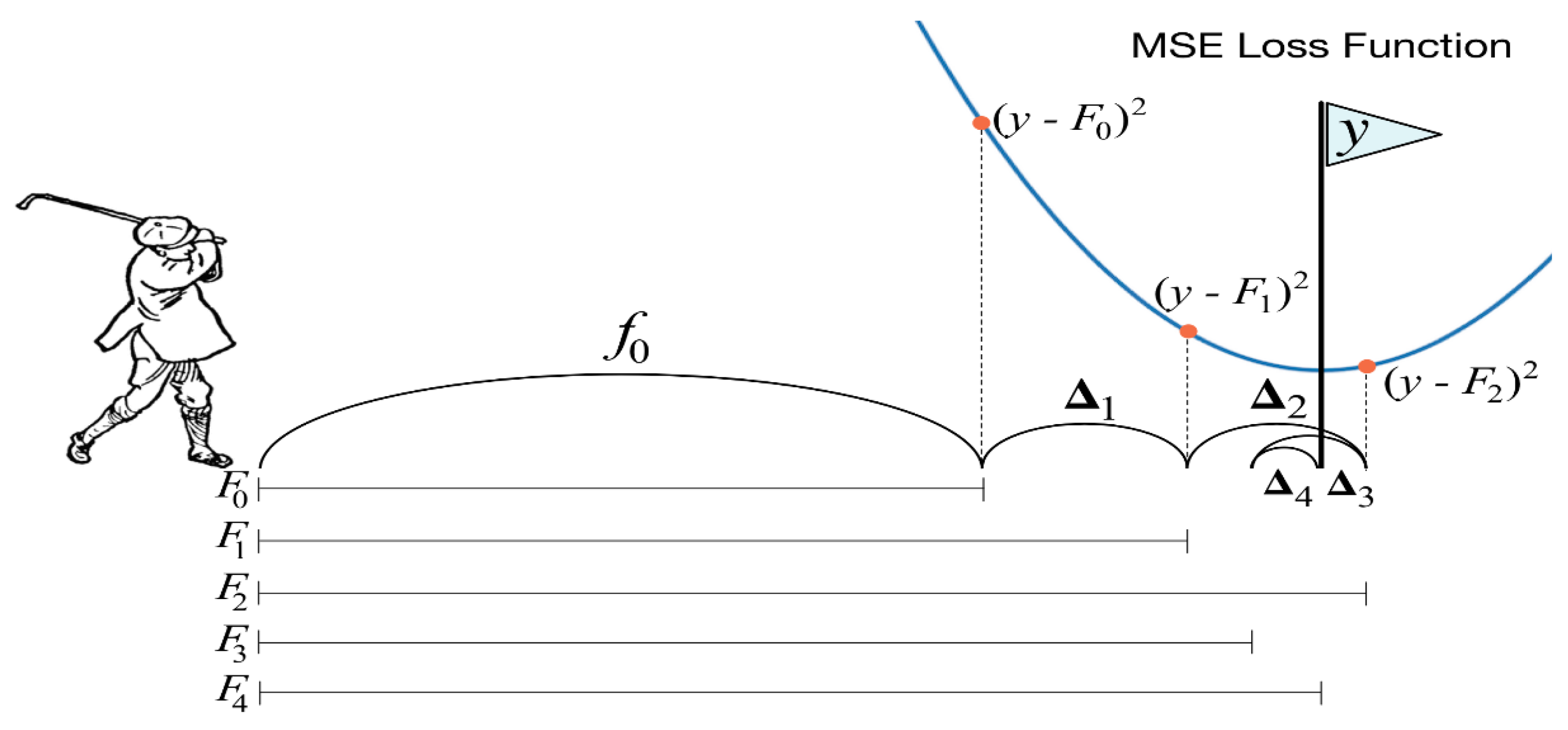
Gradient boosting is a machine learning method that uses the utilisation of additive models that undergo forward, step-by-step training. In this process, each successive model is trained to correct the residual errors of its previous models. This procedure is repeated until the predefined loss function is minimised.
In Equation (3), , x, and represent, the following decision trees of constant size, set of input variables and summation of m decision trees, respectively. To predict the response from the training set for the optimal
which results in
In Equation (5), also relates to which represents the model that adjusts to the current residuals at each iteration. It is important to acknowledge that the current residuals are defined as the negative gradients of the squared error loss function.
This also implies that is corresponding to the negative gradient of the squared error loss function. A learning rate v, known as the shrinkage factor, is introduced to scale the impact of each decision tree in the model. This regularization technique is utilized to mitigate the risk of overfitting and can be formulated as;
3.2.5. Gene Expression Programming (GEP)
GEP is an advanced technique built on the concepts of GA and GP, with the primary objective of augmenting the problem-solving capabilities of the system [46]. The five fundamental components that form GEP are the terminal set, function set, fitness function, termination condition and control parameters. GEP is predicated on the utilisation of fixed-length character strings for the purpose of depicting remedies for issues, which are subsequently visualised as parse trees.Notwithstanding, the representation of parse trees is a conventional feature of traditional GP [21].Employed character strings are +,*,*,,,,,,namely and these strings are shown in Figure 7. Additively, the representation of trees is called an expression tree and is presented in same figure.
Mathematical representation of expression tree that is shown in Figure 7, is written in the Equation (8).
The process is initiated by the random creation of chromosomes, which constitute the initial population. Subsequently, the expressed chromosomes are evaluated in order of their relative fitness. Subsequently, the selection of individuals is carried out on the basis of their suitability for reproduction with regard to modification. Until a solution is found, or for a predetermined number of generations, the procedure is repeated.[46]. Basic sequence of GEP is illustrated in the Figure 8.
The process of mathematical evolution is initiated with the generation of candidate functions, which function as initial approximations. This is followed by a series of operations, including mutation, which introduces random variations, and crossover, which combines aspects of different solutions. The final stage of the process involves the application of natural selection, a fundamental mechanism that guides the selection of the most effective candidates based on their fitness. The primary objective of this process is to refine the model, thereby achieving a close approximation to the given data. This iterative process continues until an optimal or sufficiently accurate solution is achieved. It is crucial to acknowledge that expressions can encompass constants as well, alongside functions and variables. The constants may be subject to evolution through the explicit or random assignment of values.To optimize the these constants different nonlinear algorithms can be used. Strengths and limitations of GEP is described in the Table 7.
4. Results and Discussion
Analysis carried out in this study was done by means of using R programming language, Windows-based personal computer equipped with an Intel(R) Core(TM) i5-10210U CPU @ 1.60GHz 2.11 GHz and 4 GB DDR3 RAM, and a 1 TB HDD.The process of normalisation is fundamentally concerned with the refinement of data discrepancies across various data types within a given dataset, in order to ensure data consistency whilst simultaneously optimising computational efficiency through the reduction of execution time and memory utilisation.Furthermore, it enables the evaluation of heterogeneous data within a consistent, uniform framework. To ensure that each column vector, representing different data types, is scaled within the range of [0,1], the following normalization formula can be employed for =0 and =1
In Equation (9), x stands for column vector, and related to minimum an maximum values of on the other hand and are the boundaries of distribution and is used for the normalised column vector that is converted from x [47].The performance of various statistical and artificial intelligence techniques is assessed by the use of R² and MAPE in this study. R² is a metric employed to evaluate the variation rate of the dependent variable in relation to the independent variables in the model. This metric quantifies the proportion of variability in the dependent variable that can be attributed to the model [48]. Additionally, the size of the unit of measurement has no bearing on the MAPE performance statistic. Consequently, if MAPE is found to be minimal, then the model can be considered to be accurate [49]. Formulas of R² and MAPE is given in the below,respectively.
where is actual or measured output, is predicted output, is mean of , and n indicates the number of observations [49]. To get the consistent validation, all models employed the straightforward random sampling technique. The dataset was partitioned into two subsets, with 80%allocated for training and 20% reserved for testing. This approach was applied consistently across all models to maintain reliability and comparability in performance evaluation.The MAPE and R² values for the five different methods employed in this study are given in Table 8, along with the values obtained for the training and test sets. R² values for all models are typically around 98%, based on the data shown in Table 8. The results showed that the MAPE performances for GBDT, MLR, GMDH,GEP and MLPNN were 0.827%, 0.844%, 0.844%, 0.856%, and 0.909%, respectively. Models run in 0.73 seconds for MLR, 6.99 seconds for GBDT, 47.65 seconds for GMDH, 76.48 seconds for GEP and 283.96 seconds for MLPNN networks.
As demonstrated in Table 8, when the methods are evaluated based on the lowest MAPE value and the greatest coefficient of variation value, it is evident that the GBDT method consistently results in optimal outcomes with regard to both the training and testing phases.When the Table 8 assessed in terms of computation time, the MLR model is identified as the most efficient method. The high accuracy of the results obtained using MLR suggests that the dataset exhibits a near-linear characteristic. The model’s lower memory requirements and shorter computation time are frequently cited as key reasons for its frequent preference.
In the case of MLPNN, finding the ideal quantity of neurons for the hidden layer is done by performing a search between 2 and 20 neurons. The number of neurons that minimises the residual variance is identified as the optimal number, which is found to be 8. While linear activation functions are to be employed in the output layer, logistic activation functions are applied in the hidden layer.
In GBDT algorithm,maximum number of trees is chosen as 400 , pruning of the series is performed based on the minimum absolute error and equal predictor weights are utilised.Additively, minimum size node to splitting is chosen 10, maximum splitting levels is determined 5 and maximum categories for continuous predictors is selected as 1000.
GEP is the another evaluated model in this study.The training of the model GEP comprised 1,771 generations and 120,000 evaluations of the fitness function. During the simplification phase, the model’s complexity was reduced from 23 to 17, achieved through 16 iterations. And ,generations required for the simplification is 198.However, the employment of nonlinear regression for the purpose of optimising constants did not yield any enhancement in terms of model accuracy. Generated function is given in Equation (12).
The final method evaluated for performance in the study is the GMDH. Two-variable quadratic reference functions have been implemented in GMDH networks.The equation obtained using GMDH that demonstrates the best result is as follows
5. Conclusions
The accurate forecasting of electricity consumption is of critical importance for optimising energy efficiency and operational reliability in industrial facilities that are subject to uninterrupted operation.The study utilised a dataset consisting of historical electricity consumption data of the facility, along with calendar and meteorological data considered to influence electricity consumption.This study evaluated the performance of statistical and artificial intelligence techniques, including MLR, MLP (including ANN), GMDH, GBDT and GEP, which are commonly used in the literature for forecasting applications. The five methods are assessed on the basis of R² and MAPE.According to the Table 8, ıf MAPE is the main criteria to evalute the resuls GBDT algortihm is the best choice. As demonstrated by the findings of the analyses, the optimal MAPE value belongs to the GBDT algorithm is obtained to be 0.827% . While the reduced computational time of the MLR algorithm is appealing for forecasting purposes, the GBDT algorithm is particularly advantageous due to its high probability of achieving prediction accuracy.This study plays a pivotal role in identifying the optimal algorithm for accurately estimating electricity consumption in industrial facilities operating under continuous production, where electricity consumption serves as one of the most critical inputs. Additionally, it offers a comprehensive comparison of various methods to evaluate their relative strengths and effectiveness.
Sample Availability: Restrictions apply to the data sets: The data sets presented in this article are not readily available because [the data are part of an ongoing study]. Requests to access the data sets should be directed to [Oğuzhan Timur, otimur@atu.edu.tr].
Abbreviations
The following abbreviations are used in this manuscript:
| AI | Artificial Intelligence |
| ANN | Artificial Neural Networks |
| ANFIS | Adaptive Neuro-Fuzzy Inference System |
| BT | Boosting Tree |
| EMD | Empirical Mode Decomposition |
| GA | Genetic Algorithm |
| GEP | Gene Expression Programming |
| GMDH | Group Method of Data Handling |
| GP | Genetic Programming |
| GRNN | Generalised Regression Neural Networks |
| LGBM | Light Gradient Boosting Machine |
| LTEF | Long-Term Electrical Energy Forecasting |
| LSSVM | Least Squares Support Vector Machines |
| MAE | Mean Absolute Error |
| MAPE | Mean Absolute Percentage Error |
| MARS | Multivariate Adaptive Regression Splines |
| MERRA-2 | Modern-Era Retrospective Analysis for Research and Applications, Version 2 |
| MLP | MultiLayer Perceptron |
| MLR | Multiple Linear Regression |
| MLTF | Medium-Term Electrical Energy Forecasting |
| MSE | Mean Squared Error |
| MSLR | Multiple Least Squares Regression |
| NASA | National Aeronautics and Space Administration |
| PSO | Particle Swarm Optimization |
| RMSE | Root Mean Square Error |
| SCADA | Supervisory Control and Data Acquisition |
| SCG | Scaled Conjugate Gradient |
| STEF | Short-Term Electrical Energy Forecasting |
| VSTEF | Very Short-Term Electrical Energy Forecasting |
| WD | Wavelet Decomposition |
| XGB | eXtreme Gradient Boosting |
References
- Allouhi, A.; El Fouih, Y.; Kousksou, T.A.J.; Zeraouli, Y.; Mourad, Y. Energy Consumption and Efficiency in Buildings: Current Status and Future Trends. Journal of Cleaner Production 2015, 109. [Google Scholar] [CrossRef]
- Hong, W.C. Electric load forecasting by support vector model. Applied Mathematical Modelling 2009, 33, 2444–2454. [Google Scholar] [CrossRef]
- Cecati, C.; Kolbusz, J.; Różycki, P.; Siano, P.; Wilamowski, B.M. A Novel RBF Training Algorithm for Short-Term Electric Load Forecasting and Comparative Studies. IEEE Transactions on Industrial Electronics 2015, 62, 6519–6529. [Google Scholar] [CrossRef]
- Dedinec, A.; Filiposka, S.; Dedinec, A.; Kocarev, L. Deep belief network based electricity load forecasting: An analysis of Macedonian case. Energy 2016, 115, 1688–1700. [Google Scholar] [CrossRef]
- Hong, T.; Fan, S. Probabilistic electric load forecasting: A tutorial review. International Journal of Forecasting 2016, 32, 914–938. [Google Scholar] [CrossRef]
- Kaboli, H.R.; Fallahpour, A.; Selvaraj, J.; Abd Rahim, N. Long-term electrical energy consumption formulating and forecasting via optimized gene expression programming. Energy 2017, 126. [Google Scholar] [CrossRef]
- Raza, M.Q.; Khosravi, A. A review on artificial intelligence based load demand forecasting techniques for smart grid and buildings. Renewable and Sustainable Energy Reviews 2015, 50, 1352–1372. [Google Scholar] [CrossRef]
- Bennett, C.; Stewart, R.; Lu, J. Forecasting low voltage distribution network demand profiles using a pattern recognition based expert system. Energy 2014, 67. [Google Scholar] [CrossRef]
- Schmidhuber, J. Deep Learning in Neural Networks: An Overview. Neural Networks 2014, 61. [Google Scholar] [CrossRef] [PubMed]
- Ahmad, A.; Hassan, M.Y.; Majid, M. Application of hybrid GMDH and Least Square Support Vector Machine in energy consumption forecasting. 2012, pp. 139–144. [CrossRef]
- Jinlian, L.; Yufen, Z.; Jiaxuan, L. Long and medium term power load forecasting based on a combination model of GMDH, PSO and LSSVM. 2017 29th Chinese Control And Decision Conference (CCDC), 2017, pp. 964–969. [CrossRef]
- Heydari, A.; Astiaso Garcia, D.; Keynia, F.; Bisegna, F.; Santoli, L. A novel composite neural network based method for wind and solar power forecasting in microgrids. Applied Energy 2019, 251. [Google Scholar] [CrossRef]
- Timur, O.; Zor, K.; Çelik, Ö.; Teke, A.; Ibrikci, T. Application of Statistical and Artificial Intelligence Techniques for Medium-Term Electrical Energy Forecasting: A Case Study for a Regional Hospital 2020. 8, 520–536. [CrossRef]
- Sarduy, J.R.G.; Di Santo, K.G.; Saidel, M.A. Linear and non-linear methods for prediction of peak load at University of São Paulo. Measurement 2016, 78, 187–201. [Google Scholar] [CrossRef]
- Goia, F.; Gustavsen, A. Energy performance assessment of a semi-integrated PV system in a zero emission building through periodic linear regression method. Energy Procedia 2017, 132, 586–591. [Google Scholar] [CrossRef]
- Yukseltan, E.; Yucekaya, A.; Bilge, A.H. Forecasting electricity demand for Turkey: Modeling periodic variations and demand segregation. Applied Energy 2017, 193, 287–296. [Google Scholar] [CrossRef]
- Pino-Mejías, R.; Pérez-Fargallo, A.; Rubio-Bellido, C.; Pulido-Arcas, J.A. Comparison of linear regression and artificial neural networks models to predict heating and cooling energy demand, energy consumption and CO2 emissions. Energy 2017, 118, 24–36. [Google Scholar] [CrossRef]
- Bagnasco, A.; Fresi, F.; Saviozzi, M.; Silvestro, F.; Vinci, A. Electrical consumption forecasting in hospital facilities: An application case. Energy and Buildings 2015, 103, 261–270. [Google Scholar] [CrossRef]
- Guillen Garcia, E.; Zorita, A.; Duque, O.; Morales, L.; Osornio-Rios, R.; Romero-Troncoso, R. Power Consumption Analysis of Electrical Installations at Healthcare Facility. Energies 2017, 10, 64. [Google Scholar] [CrossRef]
- Damrongsak, D.; Wongsapai, W.; Thinate, N. Factor Impacts and Target Setting of Energy Consumption in Thailand’s Hospital Building. Chemical Engineering Transactions 2018, 70, 1585–1590. [Google Scholar] [CrossRef]
- Hosseini, S.; Gandomi, A. Short-term load forecasting of power systems by gene expression programming. Neural Computing and Applications 2012, 21, 377–389. [Google Scholar] [CrossRef]
- Fan, X.; Zhu, Y. The application of Empirical Mode Decomposition and Gene Expression Programming to short-term load forecasting. 2010, Vol. 8, pp. 4331–4334. [CrossRef]
- Yin, J.; Huo, L.; Guo, L.; Hu, J. Short-term load forecasting based on improved gene expression programming. 2008 7th World Congress on Intelligent Control and Automation, 2008, pp. 5647–5650. [CrossRef]
- Bakare, M.; Abdulkarim, A.; Nuhu, A.; Muhamad, M. A hybrid long-term industrial electrical load forecasting model using optimized ANFIS with gene expression programming. Energy Reports 2024, 11. [Google Scholar] [CrossRef]
- Tabatabaei, S.; Nazeri Tahroudi, M.; Hamraz, B. Comparison of the performances of GEP, ANFIS, and SVM artifical intelligence models in rainfall simulaton. Időjárás 2021, 125, 195–209. [Google Scholar] [CrossRef]
- Jalal, F.; xu, Y.; Iqbal, M.; Javed, M.F.; Jamhiri, B. Predictive modeling of swell-strength of expansive soils using artificial intelligence approaches: ANN, ANFIS and GEP. Journal of Environmental Management 2021, 289C. [Google Scholar] [CrossRef] [PubMed]
- Kim, J.; Lee, B.; Kim, C. A Study on the development of long-term hybrid electrical load forecasting model based on MLP and statistics using massive actual data considering field applications. Electric Power Systems Research 2023, 221, 109415. [Google Scholar] [CrossRef]
- Askari, M.; Keynia, F. Mid-term Electricity Load Forecasting by a New Composite Method Based on Optimal Learning MLP Algorithm. IET Generation, Transmission & Distribution 2020, 14. [Google Scholar] [CrossRef]
- Rafati, A.; Joorabian, M.; Mashhour, E. An efficient hour-ahead electrical load forecasting method based on innovative features. Energy 2020, 201, 117511. [Google Scholar] [CrossRef]
- Massaoudi, M.S.; Refaat, S.; Chihi, I.; Trabelsi, M.; Oueslati, F.; Abu-Rub, H. A novel stacked generalization ensemble-based hybrid LGBM-XGB-MLP model for Short-Term Load Forecasting. Energy 2020, 214. [Google Scholar] [CrossRef]
- Damrongsak, D.; Wongsapai, W.; Thinate, N. Factor Impacts and Target Setting of Energy Consumption in Thailand’s Hospital Building. Chemical Engineering Transactions 2018, 70, 1585–1590. [Google Scholar] [CrossRef]
- Gordillo-Orquera, R.; Lopez-Ramos, L.M.; Muñoz-Romero, S.; Iglesias-Casarrubios, P.; Arcos-Avilés, D.; Marques, A.G.; Rojo-Álvarez, J.L. Analyzing and Forecasting Electrical Load Consumption in Healthcare Buildings. Energies 2018, 11. [Google Scholar] [CrossRef]
- Hong, T.; Gui, M.; Baran, M.; Willis, H. Modeling and forecasting hourly electric load by multiple linear regression with interactions. 2010, pp. 1 – 8. [CrossRef]
- Amral, N.; Ozveren, C.; King, D. Short term load forecasting using Multiple Linear Regression. 2007, pp. 1192 – 1198. [CrossRef]
- De Giorgi, M.G.; Malvoni, M.; Congedo, P. Comparison of strategies for multi-step ahead photovoltaic power forecasting models based on hybrid group method of data handling networks and least square support vector machine. Energy 2016, 107, 360–373. [Google Scholar] [CrossRef]
- Xiao, J.; Li, Y.; Xie, L.; Liu, D.; Huang, J. A hybrid model based on selective ensemble for energy consumption forecasting in China. Energy 2018, 159. [Google Scholar] [CrossRef]
- Dag, O.; Yozgatligil, C. GMDH: An R package for short term forecasting via GMDH-type neural network algorithms. The R Journal 2016, 8, 379–386. [Google Scholar] [CrossRef]
- Zor, K.; Çelik, Ö.; Timur, O.; Teke, A. Short-Term Building Electrical Energy Consumption Forecasting by Employing Gene Expression Programming and GMDH Networks. Energies 2020, 13. [Google Scholar] [CrossRef]
- Ishik, M.Y.; Göze, T.; Özcan, İ.; Güngör, V.Ç.; Aydın, Z. Short term electricity load forecasting: A case study of electric utility market in Turkey. 2015 3rd International Istanbul Smart Grid Congress and Fair (ICSG), 2015, pp. 1–5. [CrossRef]
- Tian, C.; Ma, J.; Zhang, C.; Zhan, P. A Deep Neural Network Model for Short-Term Load Forecast Based on Long Short-Term Memory Network and Convolutional Neural Network. Energies 2018, 11. [Google Scholar] [CrossRef]
- Wilamowski, B.M. Neural network architectures and learning algorithms. IEEE Industrial Electronics Magazine 2009, 3, 56–63. [Google Scholar] [CrossRef]
- Hochreiter, S. The Vanishing Gradient Problem During Learning Recurrent Neural Nets and Problem Solutions. International Journal of Uncertainty, Fuzziness and Knowledge-Based Systems 1998, 6, 107–116. [Google Scholar] [CrossRef]
- Touzani, S.; Granderson, J.; Fernandes, S. Gradient boosting machine for modeling the energy consumption of commercial buildings. Energy and Buildings 2017, 158. [Google Scholar] [CrossRef]
- Parr, T.; Howard, J. How to Explain Gradient Boosting: Illustration of GBDT by Golf Example, 2019.
- Persson, C.; Bacher, P.; Shiga, T.; Madsen, H. Multi-site solar power forecasting using gradient boosted regression trees. Solar Energy 2017, 150, 423–436. [Google Scholar] [CrossRef]
- Ferreira, C. Gene Expression Programming: a New Adaptive Algorithm for Solving Problems, 2001, [arXiv:cs.AI/cs/0102027].
- He, Y.; Zheng, Y. Short-term power load probability density forecasting based on Yeo-Johnson transformation quantile regression and Gaussian kernel function. Energy 2018, 154, 143–156. [Google Scholar] [CrossRef]
- Çelik, Ö.; Teke, A.; Yıldırım, B. The optimized artificial neural network model with Levenberg-Marquardt algorithm for global solar radiation estimation in Eastern Mediterranean Region of Turkey. Journal of Cleaner Production 2015, 116. [Google Scholar] [CrossRef]
- Zor, K.; Timur, O.; Çelik, Ö.; Yıldırım, B.; Teke, A. Interpretation of Error Calculation Methods in the Context of Energy Forecasting. 2017.
Figure 1.
Electric load forecasting classification.
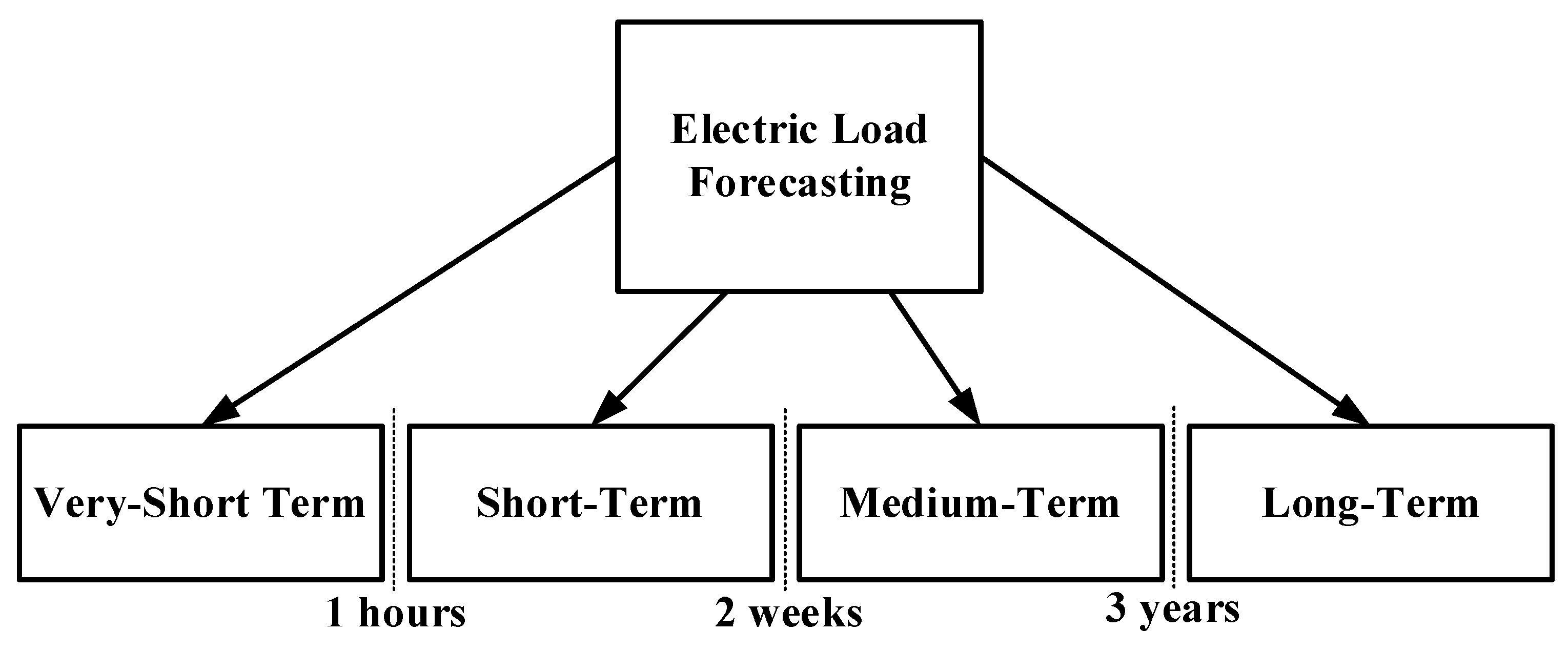
Figure 2.
Flowchart of the the study.
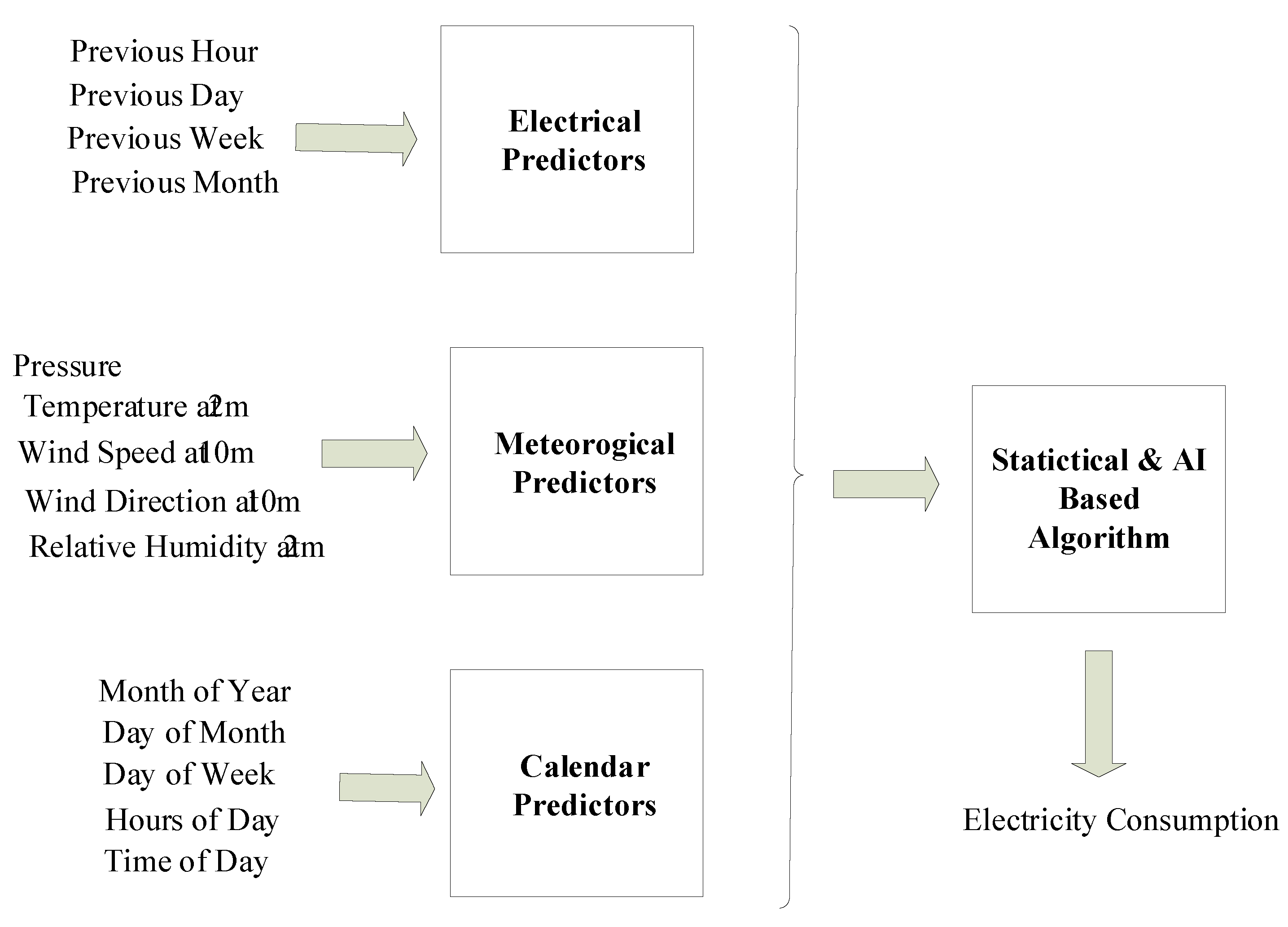
Figure 3.
Basic sequence of GMDH Algorithm [38].
Figure 3.
Basic sequence of GMDH Algorithm [38].
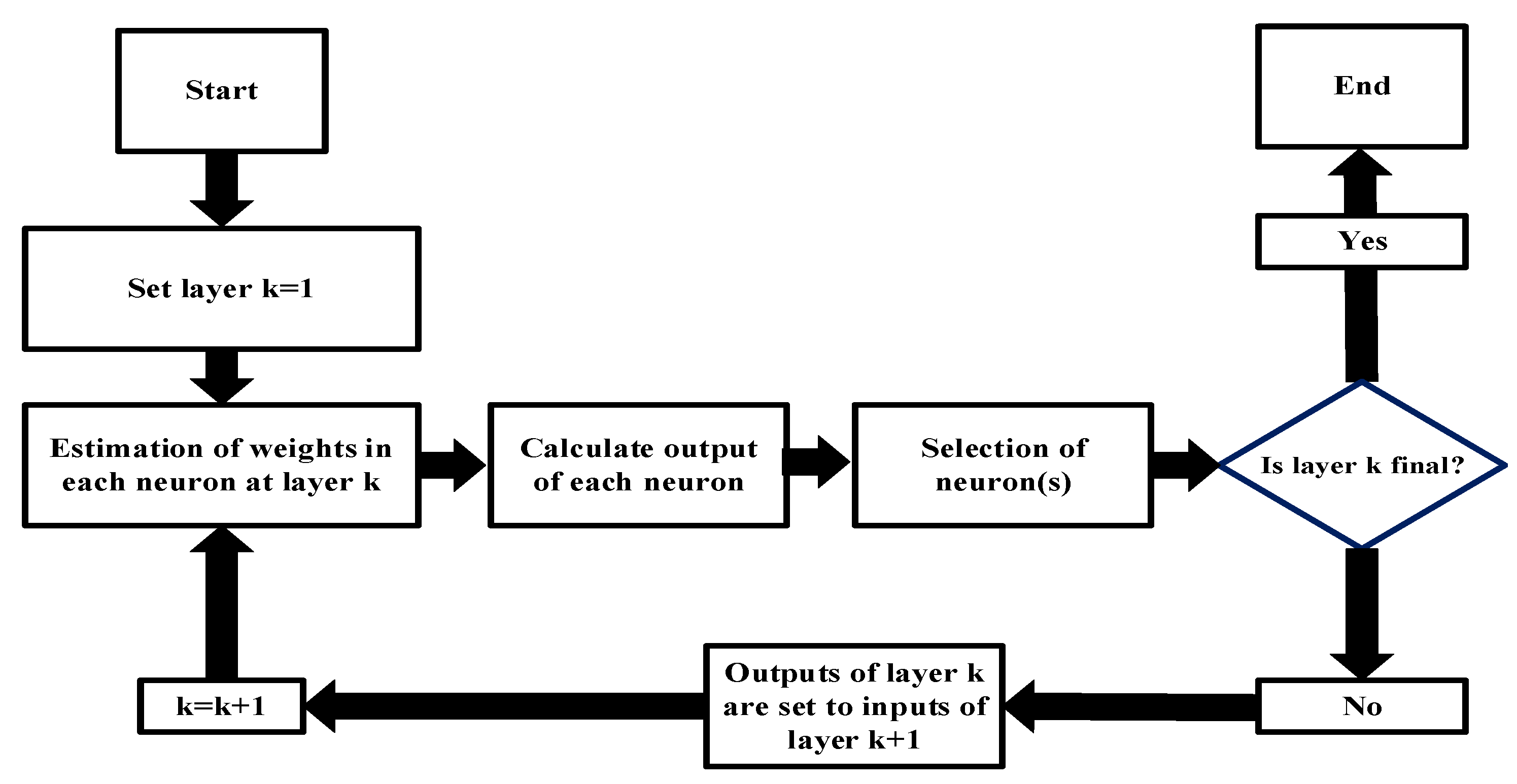
Figure 5.
A simple single hidden layer feedforward ANN topology.
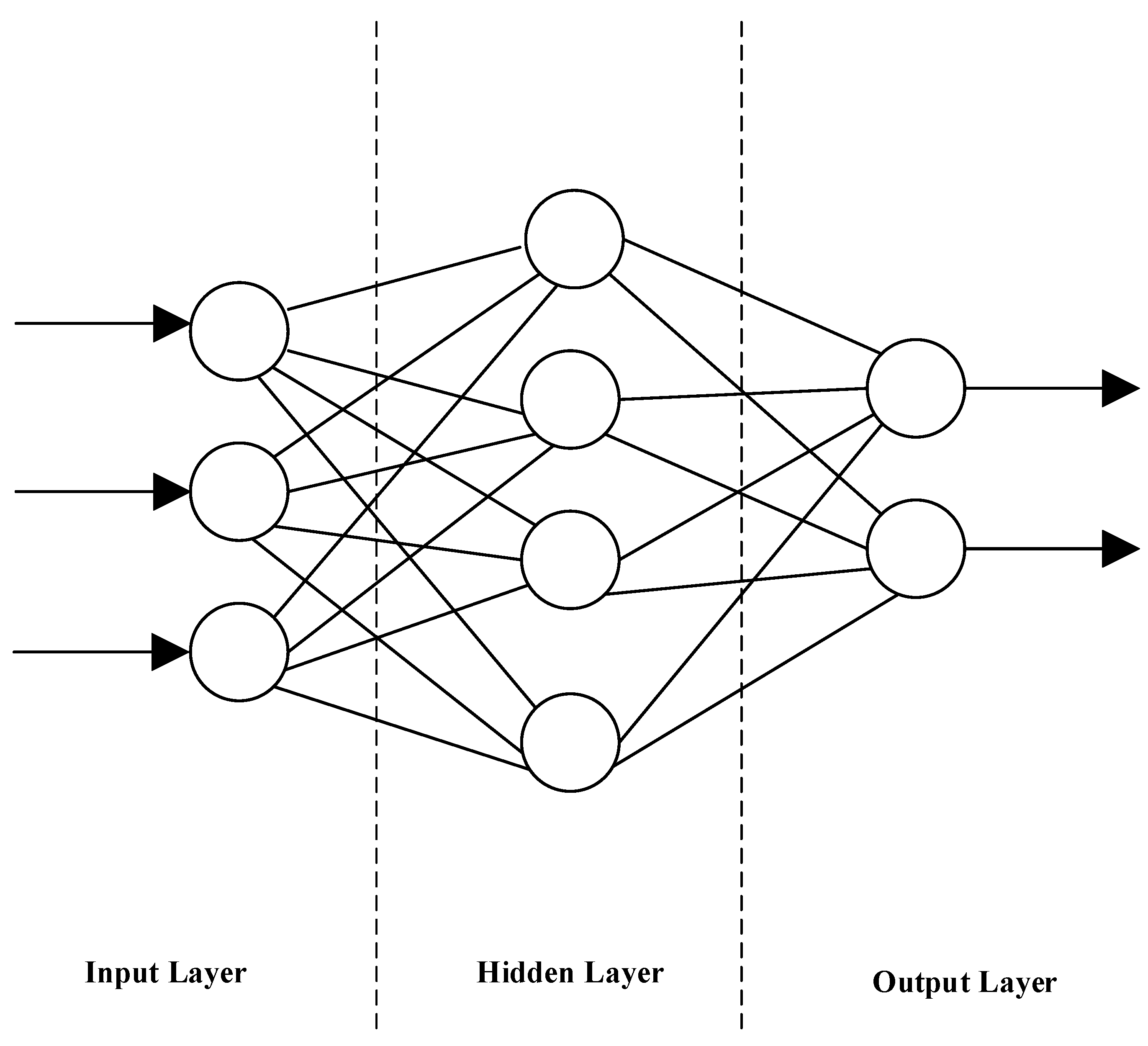
Figure 7.
Representation of expression tree
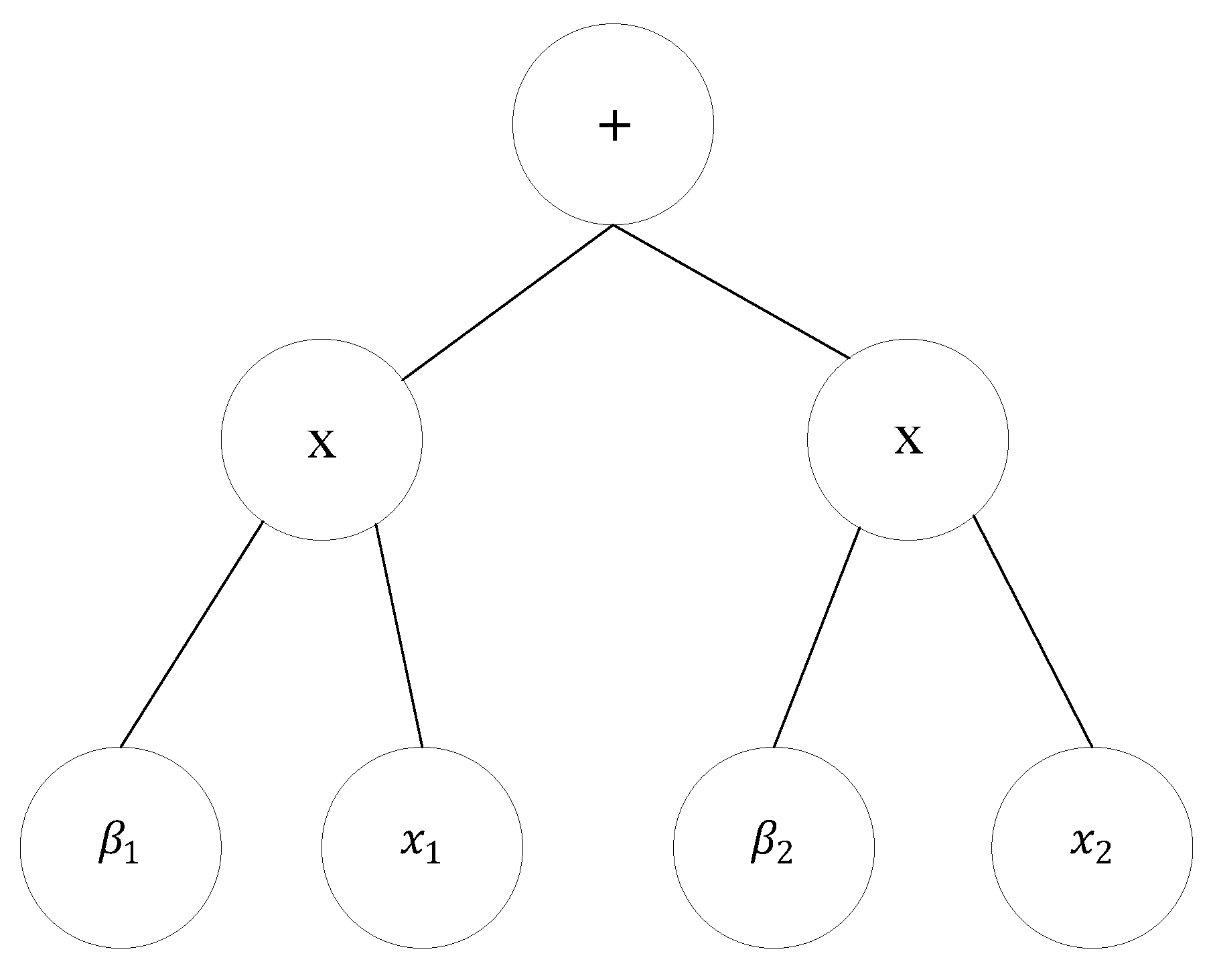
Figure 8.
Basic sequence of GEP Algorithm [38].
Figure 8.
Basic sequence of GEP Algorithm [38].
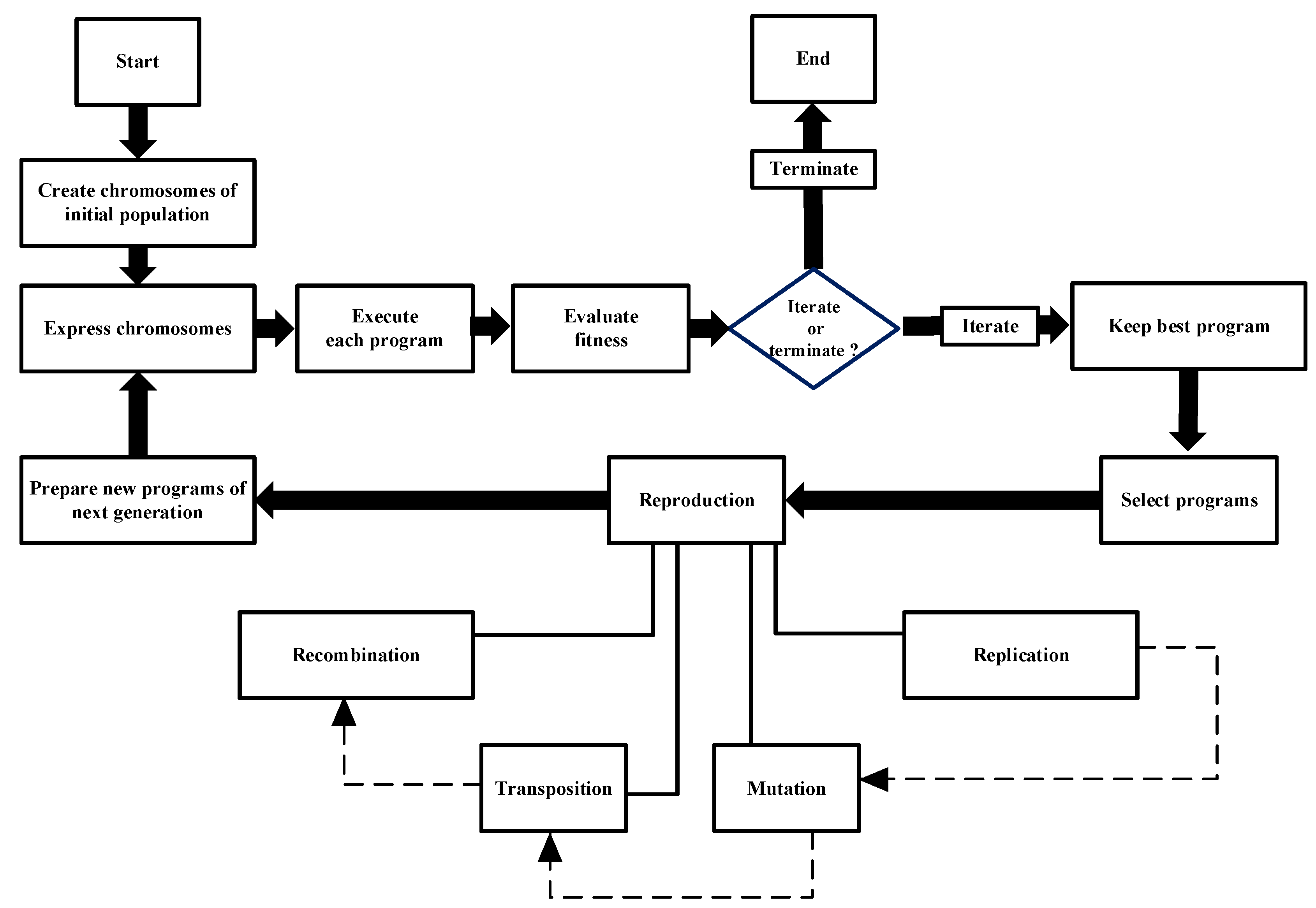

Table 1.
Applications of electric load forecasting
| Very-Short Term | Short-Term | Medium-Term | Long-Term | |
|---|---|---|---|---|
| Energy Purchasing | ✓ | ✓ | ✓ | |
| Electrical Power System Planning | ✓ | ✓ | ✓ | |
| Demand Management | ✓ | ✓ | ||
| Maintenance and Operation | ✓ | ✓ | ||
| Finance | ✓ | ✓ |
Table 2.
Specifications of Input Variables
| Category | Predictor Name | Description | Unit | Min | Median | Mean | Max |
|---|---|---|---|---|---|---|---|
| Electrical | consP1 | Previous Hour Consumption | MWh | 28.8 | 63.14 | 62.52 | 127.70 |
| consP24 | Previous Day Consumption | MWh | 28.8 | 63.14 | 62.52 | 127.70 | |
| consP168 | Previous Week Consumption | MWh | 28.7 | 63.14 | 62.52 | 127.70 | |
| consP720 | Previous Month Consumption | MWh | 28.7 | 63.14 | 62.52 | 127.70 | |
| Meteorological | T2M | Temperature at 2 Meters | °C | 3.45 | 19.47 | 19.37 | 44.47 |
| RH2M | Relative Humidity at 2 Meters | % | 5.81 | 53.50 | 53.47 | 100.00 | |
| PREC | Precipitation | mm/hour | 0.0 | 0.0 | 0.0583 | 7.90 | |
| PRES | Surface Pressure | kPa | 96.8 | 98.45 | 98.47 | 100.36 | |
| WS10M | Wind Speed at 10 Meters | m/s | 0.02 | 3.0 | 3.299 | 15.77 | |
| WD10M | Wind Direction at 10 Meters | Degrees | 0.0 | 184.375 | 185.375 | 359.93 | |
| Calendar | MoY | Month of Year | - | 1.0 | 7.0 | 6.522 | 12.0 |
| DoM | Day of Month | - | 1.0 | 16.0 | 15.75 | 31.0 | |
| DoW | Day Of Week | - | 1.0 | 4.0 | 3.99 | 7.0 | |
| HoD | Hours of Day | - | 0.0 | 11.5 | 11.49 | 23.0 | |
| ToD | Time of Day | - | 0.0 | 0.5 | 0.3187 | 1.0 |
Table 3.
Strengths and limitations of MLR
| Technique | Applied Model | Strengths | Limitations |
|---|---|---|---|
| STATISTICAL | MLR |
|
|
Table 4.
Strengths and limitations of GMDH
| Technique | Applied Model | Strengths | Limitations |
|---|---|---|---|
| AI | GMDH |
|
|
Table 5.
Strengths and limitations of MLPNN
| Technique | Applied Model | Strengths | Limitations |
|---|---|---|---|
| AI | MLPNN |
|
|
Table 6.
Strengths and limitations of GBDT
| Technique | Applied Model | Strengths | Limitations |
|---|---|---|---|
| AI | GBDT |
|
|
Table 7.
Strengths and limitations of GEP
| Technique | Applied Model | Strengths | Limitations |
|---|---|---|---|
| AI | GEP |
|
|
Table 8.
Performance results of the compared models
| Training | Test | ||||
|---|---|---|---|---|---|
| Model | R2 (%) | MAPE (%) | R2 (%) | MAPE (%) | Computational Time (s) |
| GBDT | 99.432 | 0.768 | 98.591 | 0.827 | 6.99 |
| MLR | 99.221 | 0.840 | 98.934 | 0.844 | 0.73 |
| GMDH | 99.225 | 0.843 | 98.917 | 0.844 | 47.65 |
| GEP | 99.161 | 0.836 | 98.910 | 0.856 | 76.48 |
| MLPNN | 99.214 | 0.897 | 98.912 | 0.909 | 283.96 |
Table 9.
The optimal GMDH network model’s parameters and coefficients.
| y | ||||||||
|---|---|---|---|---|---|---|---|---|
| 0.373176 | 0.995068 | -0.010423 | 0.000928 | -0.000072 | -0.001758 | |||
| -0.098162 | 0.030519 | 1.001483 | 0.000412 | -0.00089 | ||||
| 0.427163 | -0.022356 | 0.99412 | 0.000252 | 0.000264 | -0.000015 | |||
| 0.438007 | -0.018055 | 0.990181 | 0.000897 | -0.001366 | -0.000004 | |||
| -0.055873 | -0.953728 | 1.955633 | 6.915873 | -3.449387 | -3.466498 | |||
| 0.002755 | 0.001672 | 1.001275 | 0.000032 | -0.00002 | -0.000055 | |||
| 0.418694 | -0.010462 | 0.989895 | 0.000929 | -0.001762 | -0.000005 | |||
| 0.339005 | -0.01959 | 0.99359 | 0.000198 | 0.000194 | 0.000026 | |||
| -0.022724 | 4.027849 | -3.027107 | 20.15361 | -10.10289 | -10.05072 |
Disclaimer/Publisher’s Note: The statements, opinions and data contained in all publications are solely those of the individual author(s) and contributor(s) and not of MDPI and/or the editor(s). MDPI and/or the editor(s) disclaim responsibility for any injury to people or property resulting from any ideas, methods, instructions or products referred to in the content. |
© 2025 by the authors. Licensee MDPI, Basel, Switzerland. This article is an open access article distributed under the terms and conditions of the Creative Commons Attribution (CC BY) license (http://creativecommons.org/licenses/by/4.0/).
Copyright: This open access article is published under a Creative Commons CC BY 4.0 license, which permit the free download, distribution, and reuse, provided that the author and preprint are cited in any reuse.


