Submitted:
23 January 2025
Posted:
27 January 2025
You are already at the latest version
Abstract
In the calibration of cone-beam computed tomography (CBCT), two factors must be checked: the alignment of the imaging detector of the CBCT system and the effect of the slant sample platform. Earlier, we developed and validated a distinct procedure to accurately calibrate with precision any misalignment of the detector by using a cylindrical phantom with beads in a straight line, parallel to the axis of rotation of the CBCT system. Here, we generalize our earlier procedure to calibrate the CBCT system, then also detect and rectify a slight slant of the sample platform. We revise and validate our new procedure by calibrating the CBCT system, and it also determines the tilt angle between the central axis of phantom and the axis of rotation, when not 0°. The errors of misaligned angles for our new procedure are within ±0.03° which calibrates the CBCT system more precisely than our earlier work. To confirm that, we have performed a complete precise calibration of a dental CBCT system with the tilting sample platform. We also reconstruct a HA phantom in this CBCT system to analyze the quality of reconstruction. We present here a validated means to calibrate a CBCT system and rectify the effect of its tilting sample platform with good accuracy.
Keywords:
ellipse fitting
; calibration
; cone-beam computed tomography
; precision alignment loop
1. Introduction
Existing geometric calibrations rely on the decision of a parameters-set that accurately characterize the imaging system’s geometry, which is setting the axis of rotation (AOR) normal to the sample platform. The well-known calibration phantoms containing steel beads set in some special pattern are used in most geometric calibration methods. The most types of extensively used phantom includes beads in circular [1,2,3], helical [4,5], a line [6,7,8,9,10], or other special arrangements [11,12].
Shih et al. [6] proposed and validated an analytic geometric scheme to calibrate, find and correct any misalignment in the imaging detector relative to the X-ray source. Here, we modify that scheme to include rectifying images taken with a tilt in the sample platform (or holder), thus calibrating the complete cone-beam computed tomography (CBCT) system including its tilt of sample platform. We validate this new scheme by using a helical-beads phantom and a line-beads phantom, allowing a tilt between the AOR and the central axis of the phantom (AOP). Sec. 2.1 will show the dental CBCT geometry and phantoms of calibration. Sec. 2.2 will show how the beads in the two chosen phantoms can have varied rotational radii. The fundamental theorem of an ideal CBCT system, where the beads in the phantoms may have varied rotating radii will be defined in Sec. 2.3. The precise relations between minor misalignment and perfect alignment will be delineated in Sec. 2.4–the relations that provide the necessary variables to depict the misalignment to constitute the foundation of the new precision alignment loop (PAL) generalized from our earlier version [6]. Sec. 3.1 will show the criterion for validating PAL’s analytical simulations. Secs. 3.2 and 3.3 will validate the new PAL by detecting the misaligned parameter-set in the simulations for the helical-beads phantom (Sec. 3.2) and the line-beads phantom (Sec. 3.3) having a slightly tilted AOP with respect to the AOR. In our analytical simulations, we set the beads and the source of X-ray as points, and each bead was projected on a misaligned detector by stretching a line from the source to the bead to intersect the misaligned detector. Sec. 4 will present the calibrating results of a dental CBCT system using our new scheme.
2. Materials and Methods
2.1. The Dental CBCT Geometry
The dental CBCT system under study exposed in Figure 1a has a flat detector and an X-ray source on the opposite sides of a AOR mounted on a rotating gantry. The central ray from the X-ray focal point S, passes O on the AOR perpendicularly, and intersects the detector at the geometric center G, or simply “the center G”. The three points, S, O, and G lie on the system’s principal axis, the z-axis, originating from O pointing to S. The y-axis is the AOR. The x-axis with its origin at O follows the rule of right-hand screw. The distance between S and O is source-to-rotational-axis distance (SRD), and the distance between S and G is source-to-detector distance (SDD). The coordinate system that defines the detector's orientation is illustrated in Figure 1b.
In an ideally aligned system, the U’-V’-W’ coordinate, a local system, is a translation of the x-y-z coordinate, the global system, along z-axis to the detector. The position (Ui, Vj) of the (i, j)th pixel is given by U-V system, the body coordinate of detector, co-planar with the U’-V’ system. If the system is not aligned, then the misalignment (θ, φ, η) can be characterized by a rotation of the axes at the center G: slant angle η about the W’-axis, skew angle φ about the V’-axis, and tilt angle θ about the U’-axis. In a misaligned system, as θ or φ is not zero, the z-axis is not overlapping with the W’-axis. The set (UG, VG, SRD, SDD, θ, φ, η) parameterizes the CBCT system. In an ideal aligned system, (θ, φ, η) = (0, 0, 0).
A misaligned system produces distorted images. Shih et al. [6] showed to find angles (θ, φ, η) accurately with precision can revive the fidelity of image. Our current approach varies from the previous works (cited in Sec. 1) by using PAL’s iterative process that starts with a data set either from a simulation or an actual CT image to acquire the angles (θ, φ, η). The essence of PAL is exposed in Figure 2, but we modify it to include finding the tilt angle ζ between the AOP and the AOR in this study.
We calibrate the CBCT system using a cylindrical phantom of helical-beads (Figure 3a), and a cylindrical phantom of line-beads (Figure 3c).The helical-beads phantom is a cylinder of 40-mm radius having eleven 2-mm diameter steel beads evenly separated by 36° in azimuth and 10 mm in height. The line-beads phantom is a cylinder of 40-mm radius having eleven 2-mm diameter steel beads by 10 mm even spacing on a line parallel to the AOP.
We acquired a projection images-set of a calibration phantom, inverted the images, and then used a method of threshold segmentation to remove each projection’s background around beads (Figure 3b,d), then applied the center-of-mass idea to the images to calculate out the exact beads’ coordinates precisely.
2.2. Varied Rotational Radii of Beads in Phantoms
The beads on the two cylindrical phantoms shown in Figure 4 can have systematically varying radii of rotation under two conditions: 1) When the helical-beads phantom’s AOP is parallel to the AOR, but displaced by a distance c in the x-z plane as exposed in Figure 4a; the beads’ rotating radii of this phantom are within the range, rp-c to rp+c, where rp is the radius of the phantom. 2) When there is a small tilt angle ζ between the line-beads phantom’s AOP and the AOR, the beads’ rotating radii of this phantom vary as exposed in Figure 3b. The tilt angle ζ can be deliberate by Eq. (1):
where d is two adjacent beads’ vertical separation, N is the number of beads, and r1, r2, r3, …, and rN are the respective beads’ rotating radii of the line-beads phantom. Eq. (1) is also applied to the helical-beads phantom, since the first bead and the last bead are located on a line parallel to the AOP. For detecting the tilt angle accurately, it is important to setup the AOR, AOP, and the line of beads in the same plane.
The actual vertical separation d’ must be modified according to Eq. (2):
2.3. The Ideal System
As shown in our previous work [6], the projections of the rotating beads on the detector are ellipses of different eccentricities. In an ideal detector, θ = φ = η = 0. Figure 5 is a ray diagram showing points H, I, J, K, L, and M on the ideal detector (in yellow) as projections of the respective positions A, B, C, D, E, and F on a circular track traced out by a bead on the rotating phantom. The six critical projected points are sufficient to derive the equations to yield the necessary set of elliptical parameters: (UL, VL), the elliptical center; a and b, the semi-major and semi-minor axes; and η*, the slant angle of the ellipse. In an ideal detector, η* = 0.
As exposed in Figure 5a, two elliptical co-vertices J and M on the detector are the respective projected positions of C and F, therefore we have
where SJ and SM are the distances from M and J (the co-vertices) to the center G (Figure 5a), respectively, r the bead’s rotating radius, and h the distance from the rotating bead to the z-axis.
The system’s magnification factor at D, the center of bead’s circular track, M is related to the position of K, the projection of D on the detector:
where SK is the distance from K to the center G, as exposed in Figure 5a.
The magnification factor M’, at the critical positions of A, B, and E, is related to their respective projections at H, I, and L on the detector, as exposed in Figure 5b:
where δ =r2/SRD, and SL is the distance from the elliptical center L to the center G.
The semi-major axis a and the rotating radius rare related according to Eq. (7):
Since the beads’ rotating radii vary, those projected ellipses on the detector have different semi-major axes.
For the projected ellipse on the detector, the relations between ‘b’, the semi-minor axis, ‘h’, the rotating bead’s height, ‘r’, this bead’s rotating radius, and ‘SL’, the distance between L, the center of the ellipse and the center G, are described by Eq. (8).
Eq. (8) gives SL, the beads’ projected elliptical centers as a function of b/r, semi-minor axis divides by respective bead’s rotating radius, and SL = SL(b/r). The SL vs. b/r plot for the elliptical centers above and below the center G, yields VG, since all the projected ellipses’ centers constitute a vertical line, then we acquire the center G, (UG, VG), from which. After finding the center G, SK can be calculated out by Eq. (4).
If a rotating bead is on the system’s principal axis (z-axis), i.e., h = 0, then on the detector, b =0, and SL = 0; and projection is a horizontal line of length 2a passing through the center G, a crucial point on the detector. Without a bead located at h = 0, however, we can still find G by considering the following. If we plot all the projected ellipses on the U-V plane, we see the ellipses flatten as the corresponding circular track’s h approaches 0, as expected. This suggests that in a VL vs. SL plot, the ellipses will provide points to which two straight lines with opposite slopes can be fitted and they intersect at the V for G. This will be shown when we present the calibration results in Sec. 4.
As the rotating bead is closer to the z-axis, then b→0, on the detector. The elliptical parameters (UL, VL, a, b, η*) will be acquired by the linear interpolation rather than fitting an ellipse.
In an ideal detector, the vertical projected distance, Sd, between two adjacent beads’ rotating centers is the same, i.e.,
2.4. The Misaligned System
We consider the condition as η, φ, and θ ≤ 10°, then sinη~η, sinφ~φ, and sinθ~θ, cosη~cosφ~cosθ~1, and after neglecting the terms of second-order, then the simplified matrix of transformation T for a misaligned system is as:
The point (U0, V0, 0) on an aligned U’–V’–W’ local system can be translated to (U0+ V0η, –U0η + V0, –U0φ + V0θ) for a misaligned detector, with respect to the original coordinate system. (U0 + V0η, –U0η + V0, –RDD –U0φ + V0θ) are their respective global Cartesian coordinates, where RDD = SDD – SRD. The small z coordinate’s variation cause the varied magnification factor of four quadrants on a misaligned detector.
Ml and Mu are the respective magnification factors of the beads below and above z-axis:
where hl (hl< 0) and hu are the bead farthest below and farthest above z-axis, respectively. Therefore, Eq. (9), the average difference ΔSd of the vertical projected separation between two adjacent beads’ rotating centers below and above z-axis is:
where N is total bead number, (N-1)*d’ ≤ (hu–hl) ≤ ( N+1)*d’, and (hu–hl) ≈ phantom’s height. The tilt angle θ of detector is acquired from Eq. (13). N*d’ is set as the phantom’s height, since the calculated θ value and the setting value of the model are closer. Eq. (13) then acquires the tilt angle θ.
In a misaligned detector, the bead’s positions A and B have distinct magnification factors caused by the tilt angle θ and skew angle φ. The positions H and I are their respective projection on the detector. Let MA and MB be the magnification factors for the bead’s respective positions of A and B, then
In the case η = 0, θ ≠ 0, and φ ≠ 0, then the two projected elliptical vertex points H and I on the detector are as follows:
A skew angle φ in a misaligned detector will cause a slant angle η* = φ×SL/SDD of this projected ellipse. As this rotating bead is on the system’s principal axis, a horizontal line on the detector is traced out by the rotating bead, therefore η* = 0. As η ≠ 0, then η is the rotational angle about “W’-axis”, which is normal to the plane of detector, therefore η* = η at the center G. The slant angle η* in Eq. (16) is necessary to add “η” to the original η* in each ellipse, then:
which shows η* is linear to SL and detector’s skew angle φ. The slant angles η* for all projected ellipses are plotted against ‘SL’ of each respective bead to acquire the detector’s skew angle φ from the plot’s slope given by Eq. (17), and the slant angle η at the center G.
Since the first order angular approximation is used, there is larger difference between the calculated misalignment and the actual data values at larger misalignment (10°). The PAL effectively reduces those differences.
The misaligned system is calibrated by the resulting angles (θ, φ, η) to acquire a new set of the near ideal detector’s images. After that, we acquire the center G, (UG, VG), and M, the CBCT system’s magnification factor, and SRD is re-acquired from Eq. (4), but we measure SDD from the CBCT system directly.
3. Validations
3.1. The Criterion for the Validation of Analytical Simulation
PAL’s ability to detect misalignment and to restore alignment was tested on a detector of a dental CBCT having 2176×1792 pixels, with a pixel size of 0.139 mm in both dimensions. The SRD and SDD are respectively set at 430 mm and 620 mm, and SRD is re-acquired by Eq. (4). The inputs and results of these tests are presented in Secs. 3.2 and 3.3, and summarized in Tables 1 and 2, respectively. The input setting values of calibrated parameters are in bold shown in the row labeled “Model”. In the row labeled “Found” are the misalignment found by the PAL’s iterative process. PAL can accurately yield all the misalignment angles, SRD, and the geometric center (UG, VG) at once. Alignment is reached when (θ, φ, η) < 0.002° (3×10⁻⁴ rad) after calibration, as listed in the row labeled “Aligned”. For this setup, all misaligned angles will be < 0.002° after calibration.
3.2. The Helical-Beads Phantom’s AOP Has a Tilt Angle ζ from the AOR
First, the helical-beads phantom (Figure 3a) has its AOP set parallel to the AOR but offset by c = 10.0 mm (Figure 4a), after that, the AOP is tilted by a small angle ζ. Thus, the rotating radii of the beads are set from 30.0 mm to (50.0+100.0*sinζ) for all tests. The results of nine analytical simulations are exposed in Table 1. The errors in SRD are within 0.1 %, and that in (UG, VG) is within 0.5 pixels of the setting values. The errors of the misaligned angles (θ, φ, η) are within ±0.03° of the relevant setting values.
3.3. The Line-Beads Phantom’s AOP Has a Tilt Angle ζ from the AOR
The line-beads phantom is exposed in Figure 3c, and its AOP has a small tilt angle ζ from the AOR. The rotating radii of the beads (Figure 4b) are set from 40.0 mm to (40.0 + 100.0*sinζ) mm for all simulations. The results of nine analytical simulations are exposed in Table 2. The errors in SRD are within 0.1%, and that in (UG, VG) is within 0.5 pixels of the setting values. The errors of the misaligned angles (θ, φ, η) are within ±0.03° of the relevant setting values.
From the simulated tests of Table 1 and Table 2, we find the two sets of results are almost the same with negligible difference. We conclude the calibrating results are independent of the choice of those two phantoms. The error of the tilt angle ζ between the AOP and the AOR is within ±0.004°of the setting values as ζ ≤ 10°. The error of angle ζ is increasing as ζ increasing, and this error is around 0.04%.
4. Results
4.1. Our Dental CT System
Having validated the efficacy of PAL, we use it calibrate our home-made dental CBCT system with the same geometry in Sec. 3. Ellipses on the detector are traced out by phantom’s rotating beads, which form the PAL’s input data, and the output of final result is the system to remove all misalignment after calibration, i.e., (θ, φ, η) ≈ (0, 0, 0). With variances < 0.002° (3×10⁻⁵ rad).
4.2. Calibrating Our Dental CBCT System
Table 3 lists the elliptical center, (UL, VL), semi-axes a and b (in pixels), slant angle η* for each ellipse, r is each bead’s rotating radius, the value of (b/r)×SRD is the projected distance of elliptical center to geometric center G, and VK the projected distance of beads to the principal axis, all decided from the image CBCT by PAL handling directly from the calibration phantom, thus “before calibration”. In Table 3 and Table 4, each bead’s rotating radius r, varies, as we expected when the AOP has a small tilt from the AOR.
Figure 6 is derived from Table 3. Figure 6a,b yield (UG, VG); Figure 6c and Eq. (13) yield θ = -0.277°; Figure 6d and Eq. (17) yield φ = 1.169° and η = -0.292°; thus (θ, φ, η) = (-0.277°, 1.169°, -0.292°) is the misalignment from the primary calculation before calibration. Through PAL, (θ, φ, η) = (-0.231°, 1.152°, -0.291°) is the misalignment from the final calculation. After calibration, we converted the misaligned parameters into "ideal aligned parameters", and final results are exposed in Table 4 and Figure 7. From Table 4, the tilt angle ζ between AOR and the AOP can be determined:
ζ = sin-1{(51.821 - 53.646)/[(11 - 1) * 10)] } = -1.046° (±0.001°).
After calibration, the geometric center G, (UG, VG) = (1028.706, 885.237) in pixels, and the CBCT magnification factor M is 1.4328 from Eq. (4), thence the SRD is 432.474 mm; Eq. (13) gives θ=(-5×10⁻⁴)°; Eq. (17) gives φ=(1×10⁻⁸)° and η=(-3×10⁻⁸)°. The misalignment of the detector are effectively reduced from (θ, φ, η) = (-0.231°, 1.152°, -0.291°) before calibration to (θ, φ, η) = ((-5×10⁻⁴)°, (1×10⁻⁸)°, (-3×10⁻⁸)°) after calibration by PAL, and the slant angles η* of all ellipses are less than 4×10⁻⁵ rad (0.003°). The CBCT system reached within ±0.001° in all three directions of the ideal alignment after calibration.
4.3. Calibrating a Dental CBCT System with Analytical Simulation
An imitation CBCT system, similar to our dental CBCT, is calibrated to validate. The results of simulations is exposed in Table 5. The errors in SRD are within 0.01%, and that in (UG, VG) is within 0.02 pixels of the setting values. The errors of the misaligned angles (θ, φ, η) are within ±0.001° of the relevant setting values. The error of the tilt angle ζ between the AOP and the AOR is within ±0.001°of this setting value. The errors of measurement uncertainty in a real CBCT system are not included.
4.4. The Reconstructed Images of the HA Phantom
The HA phantom is designed to analyze the CT reconstruction quality. The reconstructed image of the HA phantom is exposed on Figure 8. There is blur circular edge for the reconstructed image without calibration. We do SNR and CNR analysis for image in CS region (slice number 365). Those two values are improved after calibration. The results are exposed in Table 6 and Table 7.
5. Discussions and Conclusions
Yang et al. [3] gave the errors of misaligned angles (θ, φ, η) within 0.04° and 0.1% error in SDD, but need precisely set beads’ locations and configurations, and the AOP and the AOR overlap. Our previous work [6] required only the two axes be parallel but not overlap, and the beads’ rotating radius > 10mm.
In this paper, we have revised and validated PAL, our precise calibrating algorithm, by using analytical simulations for the setting models and to calibrate a CBCT system by PAL with cylindrical phantoms of a helical-beads (Sec. 3.2) and a line-beads (Sec. 3.3), under three conditions: 1) the detector’s misaligned angles (θ, φ, η) be each<10°, to fit the first-order approximation of the trigonometric functions in Eq. (10), the transformation matrix T; 2) all critical knowledge of misalignment comes from the parameters describing the ellipses projected on the detector by the beads with varied radii of rotation about the AOR; and 3) the AOP needs not be parallel to the AOR, but any small tilt angle ζ between the two axes can be determined.
We found our new procedure to: 1) calibrate the CBCT system more precisely than our previous work [6] in the errors of misaligned angles (θ, φ, η); 2) determine the tilt angle between the AOP and AOR, when not 0°; and 3) work equally well with different phantoms. We conclude that our generalized procedure presented above can give a complete, precise characterization of any CBCT system including a tilting sample platform.
6. Acknowledgments
This work was supported in part by the grand of MOST 109-2221-E-010-019-MY2, 110-2221-E-010-019-MY2, NSTC 112-2221-EA49-050-MY2 and 112-2811-E-A49A-002. We also thank K.C. Hsieh of the University of Arizona for helpful comments and suggestions.
References
- Y. Cho, D. J. Moseley, J. H. Siewerdsen, and D. A. Jaffray, "Accurate technique for complete geometric calibration of cone-beam computed tomography systems," Medical physics, vol. 32, no. 4, pp. 968-983, 2005. [CrossRef]
- J. C. Ford, D. Zheng, and J. F. Williamson, "Estimation of CT cone-beam geometry using a novel method insensitive to phantom fabrication inaccuracy: implications for isocenter localization accuracy," Med Phys, vol. 38, no. 6, pp. 2829-40, Jun 2011. [CrossRef]
- H. Yang, K. Kang, and Y. Xing, "Geometry calibration method for a cone-beam CT system," Med Phys, vol. 44, no. 5, pp. 1692-1706, May 2017. [CrossRef]
- S. Hoppe, F. Noo, F. Dennerlein, G. Lauritsch, and J. Hornegger, "Geometric calibration of the circle-plus-arc trajectory," Phys Med Biol, vol. 52, no. 23, pp. 6943-60, Dec 7 2007. [CrossRef]
- M. Xu, C. Zhang, X. Liu, and D. Li, "Direct determination of cone-beam geometric parameters using the helical phantom," Phys Med Biol, vol. 59, no. 19, pp. 5667-90, Oct 7 2014. [CrossRef]
- K. L. Shih, D. S. Jin, Y. H. Wang, T. T. N. Tran, and J. C. Chen,"A simple and precise alignment calibration method for cone-beam computed tomography with the verifications," Phys Med Biol, Feb 15 2024. [CrossRef]
- L. von Smekal, M. Kachelriess, E. Stepina, and W. A. Kalender, "Geometric misalignment and calibration in cone-beam tomography," Med Phys, vol. 31, no. 12, pp. 3242-66, Dec 2004. [CrossRef]
- J. Xu and B. M. Tsui, "A graphical method for determining the in-plane rotation angle in geometric calibration of circular cone-beam CT systems," IEEE Trans Med Imaging, vol. 31, no. 3, pp. 825-33, Mar 2012. [CrossRef]
- J. Xu and B. M. Tsui, "An analytical geometric calibration method for circular cone-beam geometry," IEEE Trans Med Imaging, vol. 32, no. 9, pp. 1731-44, Sep 2013. [CrossRef]
- K. Yang, A. L. Kwan, D. F. Miller, and J. M. Boone, "A geometric calibration method for cone beam CT systems," Med Phys, vol. 33, no. 6, pp. 1695-706, Jun 2006. [CrossRef]
- X. Li, Z. Da, and B. Liu, "A generic geometric calibration method for tomographic imaging systems with flat-panel detectors--a detailed implementation guide," Med Phys, vol. 37, no. 7, pp. 3844-54, Jul 2010. [CrossRef]
- C. Mennessier, R. Clackdoyle, and F. Noo, "Direct determination of geometric alignment parameters for cone-beam scanners," Phys Med Biol, vol. 54, no. 6, pp. 1633-60, Mar 21 2009. [CrossRef]
Figure 1.
(a) The dental CBCT geometry. S stands for the X-ray point source, O is on the axis of rotation, and G is the detector’s geometrical center. The x-axis points into the y-z plane which is not shown. (b) (θ, φ, η) are the three tilt angles of detector’s local U’-V’-W’ coordinate at G.
Figure 1.
(a) The dental CBCT geometry. S stands for the X-ray point source, O is on the axis of rotation, and G is the detector’s geometrical center. The x-axis points into the y-z plane which is not shown. (b) (θ, φ, η) are the three tilt angles of detector’s local U’-V’-W’ coordinate at G.
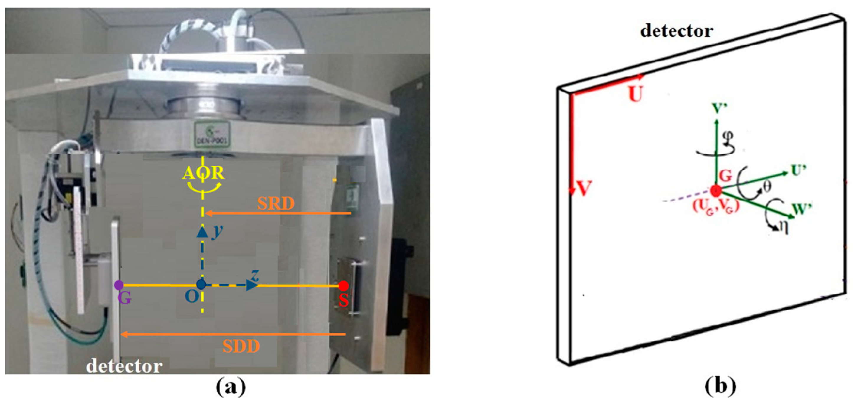
Figure 2.
The PAL’s flowchart.
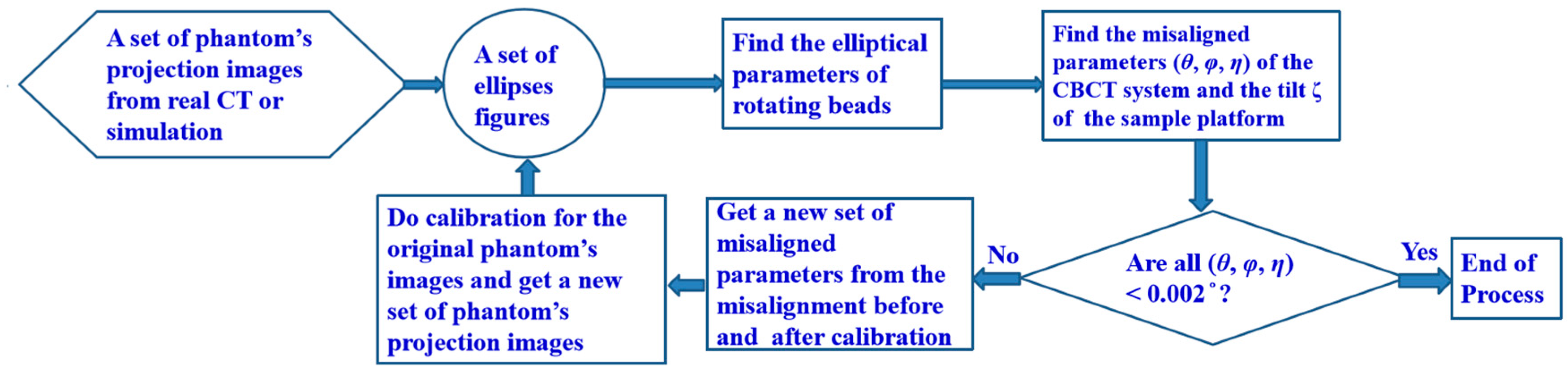
Figure 3.
(a) The helical-beads phantom. (b) The inverted projection of helical-beads phantom after removing the background around the beads. (c) The line-beads phantom. (d) The inverted projection of line-beads phantom after removing the background around the beads.
Figure 3.
(a) The helical-beads phantom. (b) The inverted projection of helical-beads phantom after removing the background around the beads. (c) The line-beads phantom. (d) The inverted projection of line-beads phantom after removing the background around the beads.
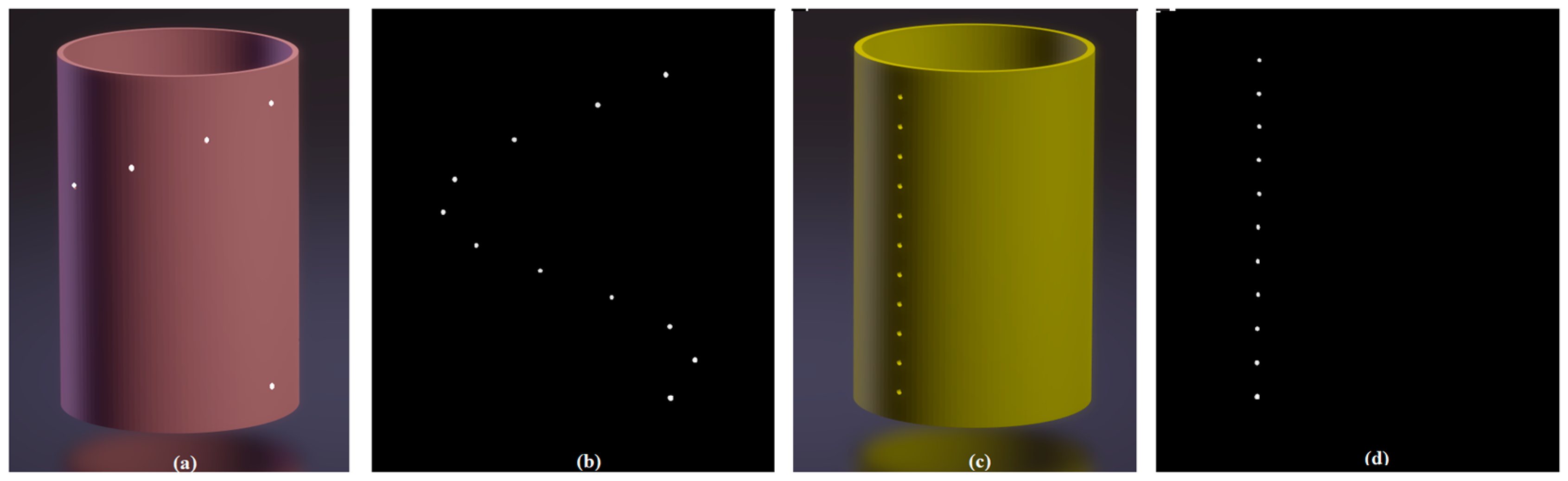
Figure 4.
Two cases of varying radii of rotation. (a) When the helical-beads phantom’s AOP parallels AOR, but displaced. (b) When the line-beads phantom’s AOP has a tilt angle ζ from the AOR, where ri is the ith bead’s rotational radius, d is two adjacent beads’ vertical separation, and N is the number of beads.
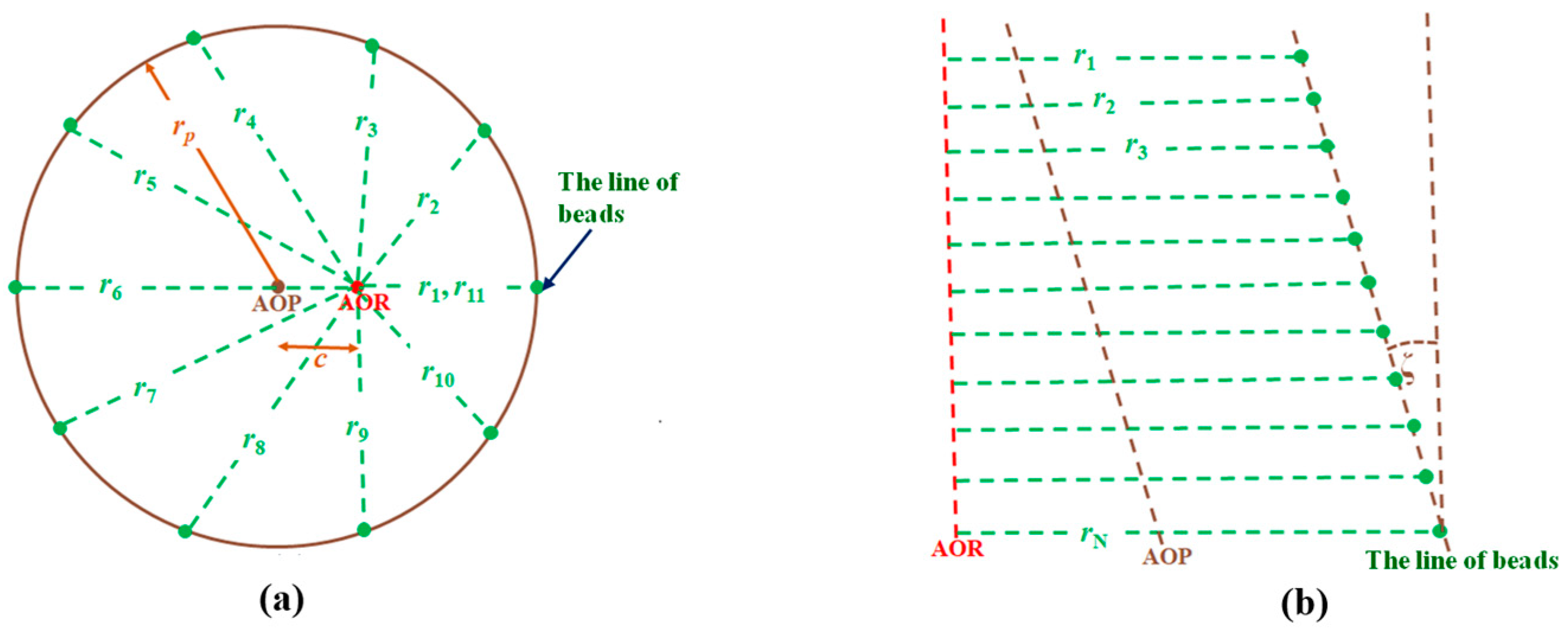
Figure 5.
Two views of the projections on the detector (in yellow) of the critical points on a circular track of radius r of a bead rotating about the AOR for an ideal system. (a) J and M on the detector are the respective projected positions of C and F on the bead’s circular track at y = h. K is the projection of D, the center of the circular track. (b) Critical points A and B on the bead’s circular track in the x-z plane have their projections H and I, respectively. The six critical points’ coordinates on the bead’s circular track are exposed on the figure, where δ=r2/SRD.
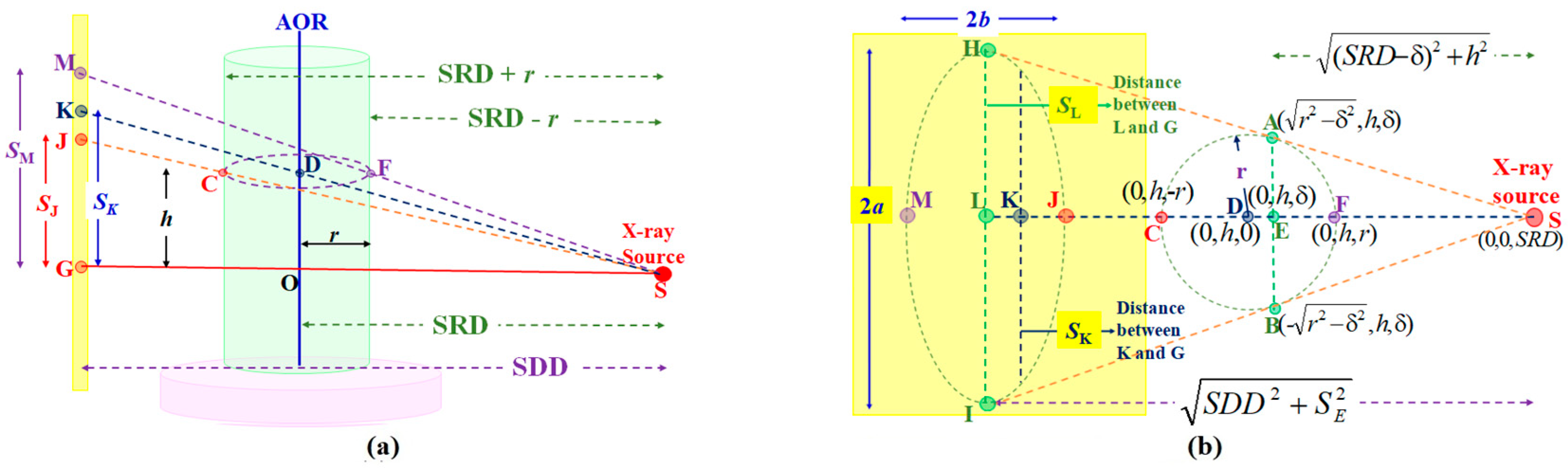
Figure 6.
The primary calculated parameters of our dental CBCT system before calibration. (a) The ellipse center’s position VL vs. (b/r)*SRD. (b) The elliptical centers are exposed in V-U coordinates. (c) The projected rotational centers VK vs. the bead number below and above z-axis. (d) The elliptical skew angle η* vs. VL.
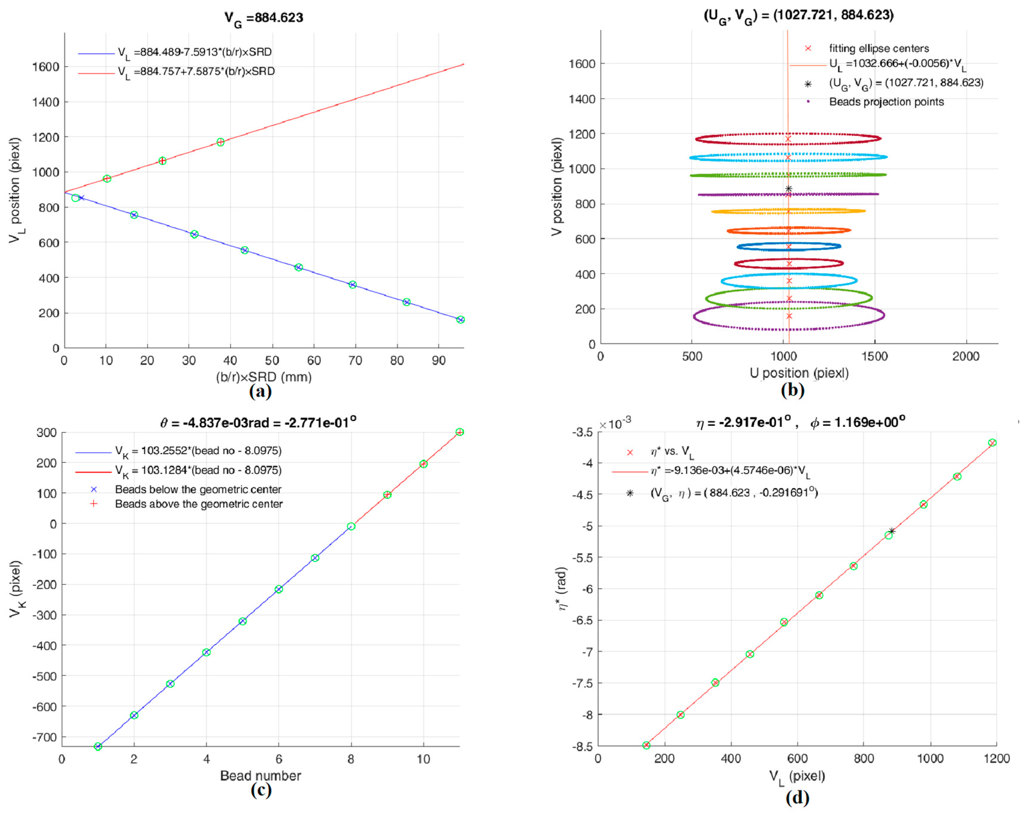
Figure 7.
The final calculated parameters of our dental CBCT system after calibration. (a) The ellipse center’s position VL vs. (b/r)*SRD. (b) The elliptical centers are exposed in V-U coordinates. (c) The projected rotational centers VK vs. the bead number below and above z-axis. (d) The elliptical skew angle η* vs. VL.
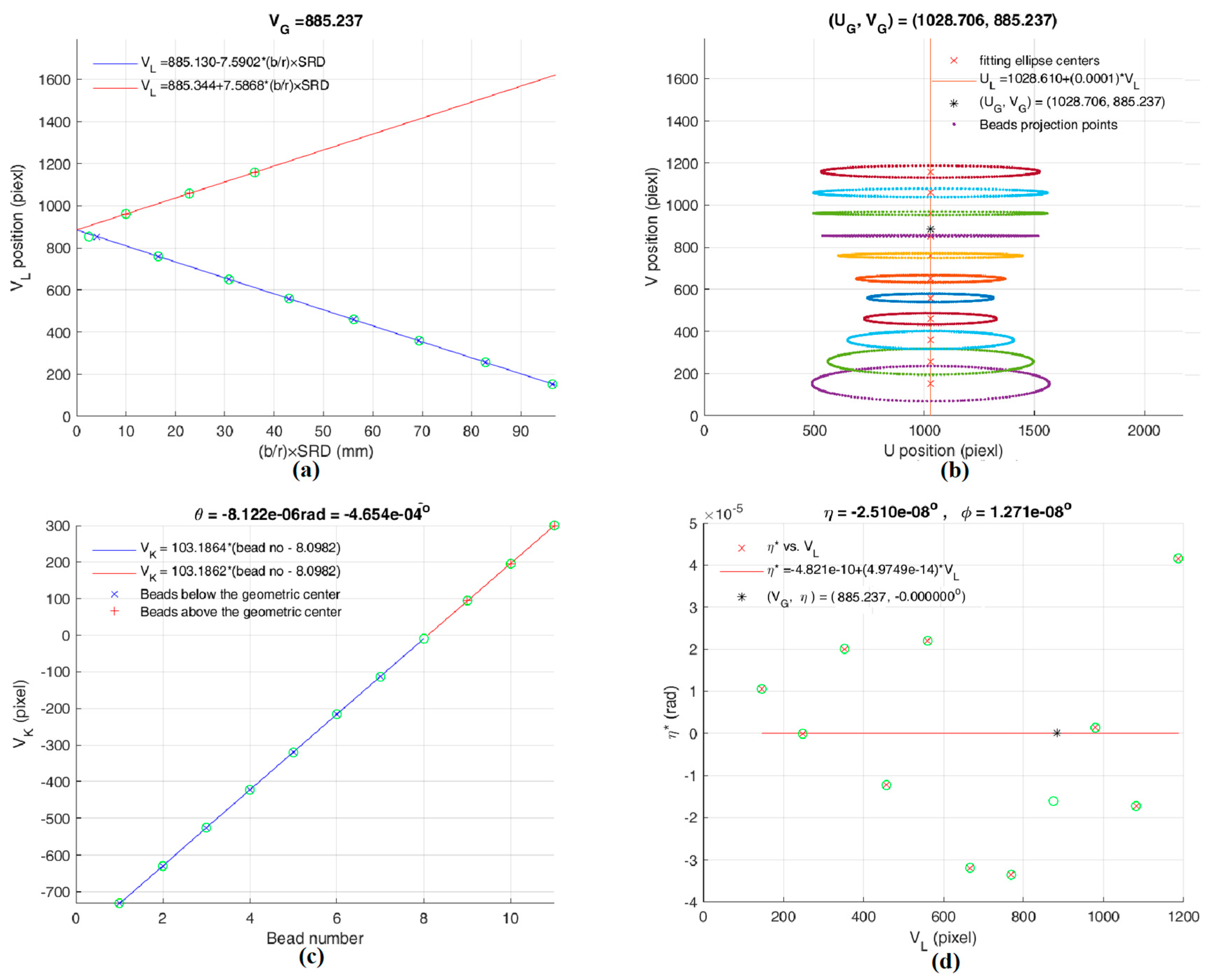
Figure 8.
The HA phantom and its reconstructed images. (a) The top view of HA phantom. (b) The side view of HA phantom. (c) The reconstructed image of slice number 365 without calibration (CS region). (d) The reconstructed image of slice number 365 with calibration (CS region). (e) The reconstructed image of slice number 775 without calibration (HA region). (f) The reconstructed image of slice number 775 with calibration (HA region). (g) The reconstructed image of slice number 850 without calibration (water region). (h) The reconstructed image of slice number 850 with calibration (water region).
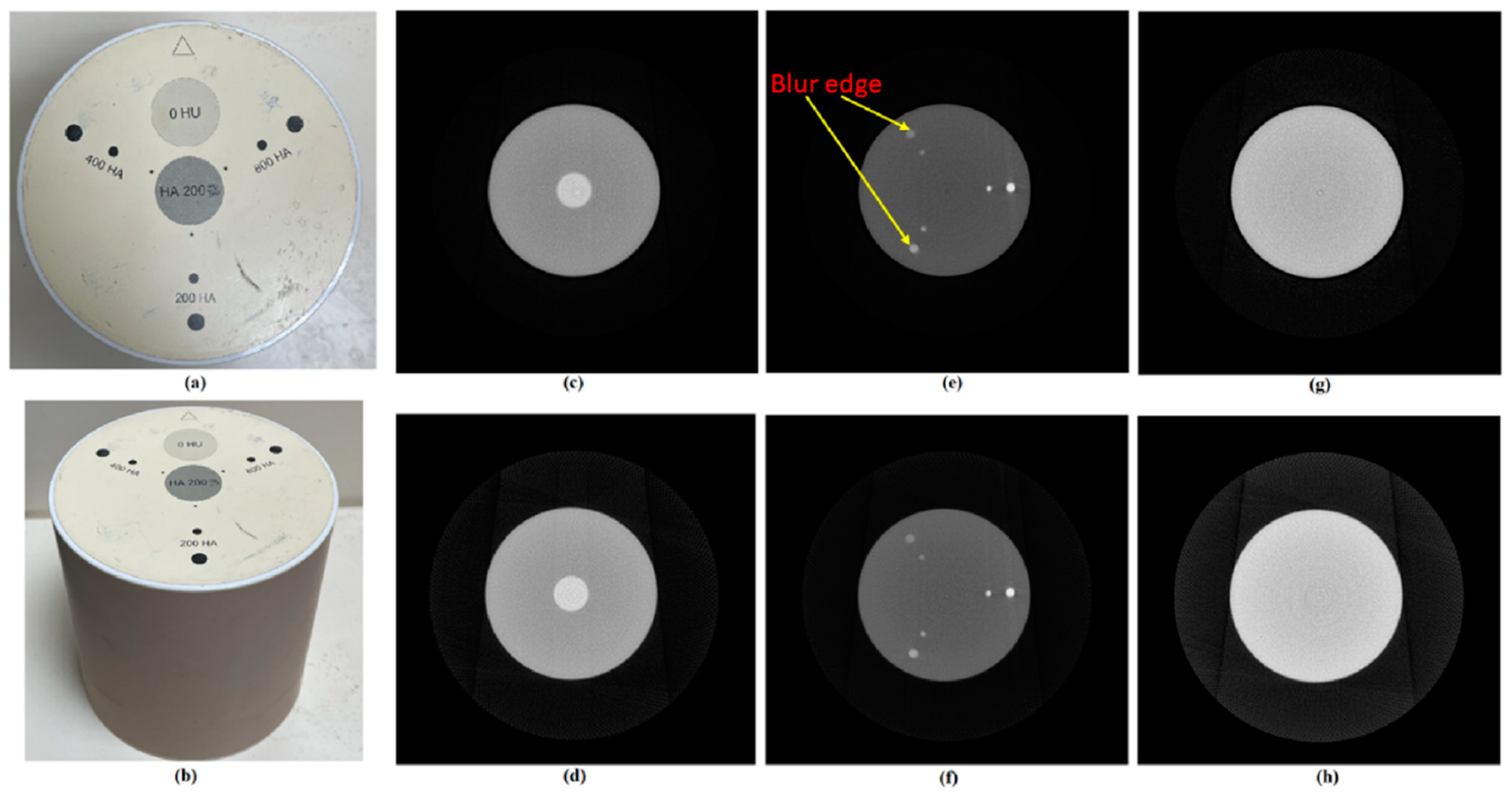

Table 1.
The analytical simulations validation when the helical-beads phantom’s AOP has a tilt angle ζ from the AOR.
Table 1.
The analytical simulations validation when the helical-beads phantom’s AOP has a tilt angle ζ from the AOR.
| Simulating Setups | UG (pixel) | VG (pixel) | SRD (mm) | θ (o) | φ(o) | η(o) | ζ(o) | Verification |
| 1 | 1000.000 | 800.000 | 430.000 | 10.000 | 0.000 | 0.000 | 2.000 | Model |
| 1000.000 | 798.519 | 421.356 | 9.999 | 0.000 | 0.000 | 2.699 | Found | |
| 1000.325 | 800.349 | 429.939 | -0.001 | 0.000 | 0.000 | 2.000 | Aligned | |
| 2 | 1000.000 | 900.000 | 430.000 | 0.000 | 10.000 | 0.000 | 3.000 | Model |
| 991.696 | 899.983 | 429.980 | 0.000 | 10.000 | 0.001 | 3.049 | Found | |
| 999.700 | 900.014 | 430.016 | 0.000 | 0.000 | 0.000 | 3.000 | Aligned | |
| 3 | 1000.000 | 1000.000 | 430.000 | 0.000 | 0.000 | 10.000 | 4.000 | Model |
| 1019.396 | 996.336 | 436.595 | 0.000 | 0.000 | 10.000 | 4.061 | Found | |
| 1000.000 | 1000.000 | 429.995 | 0.000 | 0.000 | 0.000 | 4.000 | Aligned | |
| 4 | 1100.000 | 800.000 | 430.000 | 1.000 | 1.000 | 1.000 | 5.000 | Model |
| 1097.653 | 799.806 | 429.764 | 1.000 | 1.000 | 1.000 | 5.079 | Found | |
| 1099.995 | 800.041 | 429.987 | 0.000 | 0.000 | 0.000 | 5.000 | Aligned | |
| 5 | 1100.000 | 900.000 | 430.000 | 2.000 | 2.000 | 2.000 | 6.000 | Model |
| 1098.800 | 899.642 | 429.497 | 2.001 | 2.000 | 2.000 | 6.163 | Found | |
| 1099.999 | 900.000 | 429.974 | 0.000 | 0.000 | 0.000 | 6.000 | Aligned | |
| 6 | 1100.000 | 1000.000 | 430.000 | 3.000 | 3.000 | 3.000 | 7.000 | Model |
| 1103.442 | 999.502 | 429.186 | 3.004 | 3.000 | 3.000 | 7.254 | Found | |
| 1100.012 | 1000.112 | 429.953 | 0.000 | 0.000 | 0.000 | 6.999 | Aligned | |
| 7 | 1200.000 | 800.000 | 430.000 | 4.000 | 4.000 | 4.000 | 8.000 | Model |
| 1190.606 | 792.391 | 428.821 | 4.010 | 4.000 | 4.009 | 8.351 | Found | |
| 1199.638 | 800.312 | 429.913 | 0.000 | 0.001 | -0.000 | 7.999 | Aligned | |
| 8 | 1200.000 | 900.000 | 430.000 | 5.000 | 5.000 | 5.000 | 9.000 | Model |
| 1196.989 | 890.534 | 428.389 | 5.019 | 5.001 | 5.012 | 9.455 | Found | |
| 1199.766 | 899.992 | 429.872 | 0.000 | 0.001 | 0.000 | 8.998 | Aligned | |
| 9 | 1200.000 | 1000.000 | 430.000 | 6.000 | 6.000 | 6.000 | 10.000 | Model |
| 1206.877 | 988.686 | 427.876 | 6.030 | 6.000 | 6.000 | 10.567 | Found | |
| 1199.983 | 999.978 | 429.815 | 0.000 | 0.001 | -0.001 | 9.996 | Aligned |
Table 2.
The analytical simulations validation when the line-beads phantom’s AOP has a tilt angle ζ from the AOR.
Table 2.
The analytical simulations validation when the line-beads phantom’s AOP has a tilt angle ζ from the AOR.
| Simulating Setups | UG (pixel) | VG (pixel) | SRD (mm) | θ (o) | φ(o) | η(o) | ζ(o) | Verification |
| 1 | 1000.000 | 800.000 | 430.000 | 10.000 | 0.000 | 0.000 | 2.000 | Model |
| 1000.000 | 798.519 | 421.272 | 9.999 | 0.000 | 0.000 | 2.930 | Found | |
| 1000.325 | 800.349 | 429.938 | 0.000 | 0.000 | 0.000 | 2.000 | Aligned | |
| 2 | 1000.000 | 900.000 | 430.000 | 0.000 | 10.000 | 0.000 | 3.000 | Model |
| 990.802 | 899.980 | 429.982 | 0.000 | 10.000 | 0.001 | 3.050 | Found | |
| 999.700 | 900.014 | 430.015 | 0.000 | 0.000 | 0.000 | 3.000 | Aligned | |
| 3 | 1000.000 | 1000.000 | 430.000 | 0.000 | 0.000 | 10.000 | 4.000 | Model |
| 1019.396 | 1013.701 | 436.595 | 0.000 | 0.000 | 10.000 | 4.061 | Found | |
| 1000.000 | 1000.000 | 429.995 | 0.000 | 0.000 | 0.000 | 4.000 | Aligned | |
| 4 | 1100.000 | 800.000 | 430.000 | 1.000 | 1.000 | 1.000 | 5.000 | Model |
| 1097.499 | 799.805 | 429.748 | 1.000 | 1.000 | 1.000 | 5.102 | Found | |
| 1099.994 | 800.041 | 429.989 | 0.000 | 0.000 | 0.000 | 5.000 | Aligned | |
| 5 | 1100.000 | 900.000 | 430.000 | 2.000 | 2.000 | 2.000 | 6.000 | Model |
| 1098.425 | 899.639 | 429.457 | 2.001 | 2.000 | 2.000 | 6.209 | Found | |
| 1099.999 | 900.000 | 429.971 | 0.000 | 0.000 | 0.000 | 6.000 | Aligned | |
| 6 | 1100.000 | 1000.000 | 430.000 | 3.000 | 3.000 | 3.000 | 7.000 | Model |
| 1102.779 | 999.507 | 429.111 | 3.004 | 3.000 | 3.000 | 7.254 | Found | |
| 1100.008 | 1000.120 | 429.922 | 0.000 | 0.000 | 0.000 | 7.000 | Aligned | |
| 7 | 1200.000 | 800.000 | 430.000 | 4.000 | 4.000 | 4.000 | 8.000 | Model |
| 1189.585 | 792.419 | 428.700 | 4.009 | 4.000 | 4.008 | 8.442 | Found | |
| 1199.634 | 800.297 | 429.846 | -0.001 | 0.001 | 0.000 | 7.997 | Aligned | |
| 8 | 1200.000 | 900.000 | 430.000 | 5.000 | 5.000 | 5.000 | 9.000 | Model |
| 1195.542 | 890.607 | 428.211 | 5.016 | 5.000 | 5.011 | 9.569 | Found | |
| 1199.790 | 899.993 | 429.704 | 0.000 | 0.000 | 0.000 | 8.996 | Aligned | |
| 9 | 1200.000 | 1000.000 | 430.000 | 6.000 | 6.000 | 6.000 | 10.000 | Model |
| 1204.934 | 988.834 | 427.627 | 6.025 | 5.999 | 6.014 | 10.703 | Found | |
| 1200.017 | 1000.059 | 429.825 | 0.000 | 0.001 | 0.000 | 9.996 | Aligned |
Table 3.
The elliptical parameters of each bead for our dental CBCT system before calibration.
| Bead No. | UL(pixel) | VL(pixel) | Semi-major axis (a) | Semi-minor axis (b) | η* (rad) | r(mm) | (b/r)*SRD(mm) | VK(pixel) |
| 1 | 1031.2101 | 160.3275 | 519.8593 | 79.3203 | -0.00849 | 51.8307 | 97.3269 | -731.5368 |
| 2 | 1031.0564 | 260.2956 | 451.6038 | 59.6192 | -0.00801 | 45.0998 | 83.8444 | -630.1795 |
| 3 | 1030.7361 | 359.1330 | 367.5386 | 40.9339 | -0.00749 | 36.7676 | 70.1228 | -526.6523 |
| 4 | 1030.4389 | 457.8673 | 294.6665 | 26.7232 | -0.00704 | 29.5132 | 56.3831 | -423.1621 |
| 5 | 1030.0572 | 555.1430 | 281.1494 | 19.6407 | -0.00653 | 28.1648 | 42.7870 | -321.1075 |
| 6 | 1029.5691 | 646.3118 | 333.6322 | 16.7880 | -0.00611 | 33.3955 | 28.8167 | -216.1962 |
| 7 | 1028.6118 | 756.4342 | 414.7303 | 11.2045 | -0.00564 | 41.4503 | 15.2588 | -114.1042 |
| 8 | 1026.8056 | 852.3691 | 489.3404 | 3.3211 | -0.00515 | 48.8252 | 1.3589 | -9.9114 |
| 9 | 1027.8958 | 962.8579 | 534.0376 | 8.8082 | -0.00466 | 53.2246 | 12.4251 | 94.2877 |
| 10 | 1026.5521 | 1064.1786 | 537.0056 | 20.3251 | -0.00422 | 53.5162 | 25.8672 | 195.0878 |
| 11 | 1025.8983 | 1169.7566 | 503.9358 | 30.3415 | -0.00368 | 50.2634 | 39.3870 | 299.6775 |
Table 4.
The elliptical parameters of each bead for our dental CBCT system after calibration.
| Bead No. | UL(pixel) | VL(pixel) | Semi-major axis (a) | Semi-minor axis (b) | η* (rad) | r(mm) | (b/r)*SRD(mm) | VK(pixel) |
| 1 | 1028.6660 | 152.4467 | 539.6596 | 83.2825 | 0.00001 | 53.6460 | 97.2815 | -731.0551 |
| 2 | 1028.7245 | 257.0081 | 466.3374 | 61.9410 | 0.00000 | 45.8087 | 83.8129 | -629.8214 |
| 3 | 1028.5931 | 359.2661 | 377.5675 | 42.0892 | 0.00002 | 36.1071 | 70.1027 | -526.3997 |
| 4 | 1028.5849 | 460.3167 | 301.1520 | 27.1958 | -0.00001 | 27.6604 | 56.3723 | -422.9981 |
| 5 | 1028.6759 | 558.8318 | 285.8904 | 19.7872 | 0.00002 | 26.0904 | 42.7827 | -321.0099 |
| 6 | 1028.8164 | 650.2557 | 337.6639 | 16.7547 | -0.00003 | 32.1808 | 28.8166 | -216.1482 |
| 7 | 1028.7173 | 759.5510 | 417.3701 | 11.0565 | -0.00003 | 41.5594 | 15.2604 | -114.0851 |
| 8 | 1027.7668 | 853.7684 | 489.5930 | 3.2483 | -0.00002 | 50.1466 | 1.3614 | -9.8960 |
| 9 | 1029.6001 | 961.1178 | 531.7960 | 8.5112 | 0.00000 | 55.2690 | 12.4292 | 94.2989 |
| 10 | 1028.8055 | 1058.5057 | 532.0376 | 19.4388 | -0.00002 | 55.6084 | 25.8771 | 195.1268 |
| 11 | 1028.5440 | 1158.9218 | 496.6324 | 28.7115 | 0.00004 | 51.8211 | 39.4054 | 299.7656 |
Table 5.
The validation of the analytical simulation for our dental CBCT system.
| Simulating Setups | UG (pixel) | VG (pixel) | SRD (mm) | θ(o) | φ(o) | η(o) | ζ(o) | Verification |
| 1 | 1029.000 | 885.000 | 432.000 | -0.230 | 1.150 | -0.290 | -1.046 | Model |
| 1028.193 | 884.699 | 432.038 | -0.230 | 1.150 | -0.290 | -1.072 | Found | |
| 1028.984 | 884.997 | 432.000 | -2×10⁻⁵ | 1×10⁻⁴ | -1×10⁻⁴ | -1.046 | Aligned |
Table 6.
The SNR and CNR for the reconstructed image without calibration of slice no. 365.
| Center | Up | Down | Left | Right | |
| SNR | 5.4567 | 4.4587 | 4.4811 | 4.4994 | 4.4583 |
| CNR | / | 1.3055 | 1.3055 | 1.2839 | 1.2846 |
Table 7.
The SNR and CNR for the reconstructed image with calibration of slice no. 365.
| Center | Up | Down | Left | Right | |
| SNR | 7.0657 | 6.8115 | 6.7803 | 6.8228 | 6.8339 |
| CNR | / | 1.5661 | 1.5603 | 1.5449 | 1.5483 |
Disclaimer/Publisher’s Note: The statements, opinions and data contained in all publications are solely those of the individual author(s) and contributor(s) and not of MDPI and/or the editor(s). MDPI and/or the editor(s) disclaim responsibility for any injury to people or property resulting from any ideas, methods, instructions or products referred to in the content. |
© 2025 by the authors. Licensee MDPI, Basel, Switzerland. This article is an open access article distributed under the terms and conditions of the Creative Commons Attribution (CC BY) license (http://creativecommons.org/licenses/by/4.0/).
Copyright: This open access article is published under a Creative Commons CC BY 4.0 license, which permit the free download, distribution, and reuse, provided that the author and preprint are cited in any reuse.


