
Submitted:
25 January 2025
Posted:
27 January 2025
You are already at the latest version
Abstract
This study evaluated heavy metal (HM) contamination in sediments from the Malbasag River in Ormoc City Port, Leyte, Philippines. A total of thirty sediment samples were collected randomly from ten locations along the river using an Ekman grab sampler. Atomic absorption spectrophotometry revealed HM concentrations in the order of Mn > Zn > Cu > Ni > Pb > Cd. All HMs exceeded sediment quality guideline (SQG) thresholds except for Mn. Contamination was assessed using indices such as the contamination factor (CF), pollution load index (PLI), geo-accumulation index (Igeo), and enrichment factor (EF). The CF values indicated “moderate to considerable” contamination for Zn, Ni, and Cd, while Cu and Pb showed “very high” contamination levels. The PLI results indicated severe sediment degradation in 20% of samples. The Igeo analysis classified 60% of the samples as “heavily to extremely polluted” for Cd, Cu, and Pb. EF analysis suggested that anthropogenic sources contributed to elevated HM levels, including port activities and agricultural runoff. Ecological risk index (RI) analysis revealed moderate risk in 40% and considerable risk in 20% of sampling locations. Multivariate analyses suggested significant anthropogenic contributions to HM contamination, highlighting the need for further studies to assess the ecological impacts.
Keywords:
Anthropogenic activities
; Heavy metals
; urban river sediment
; pollution indices
; ecological risk
; multivariate statistical methods
Highlights
- • The first study focused on the concentrations of heavy metals (Cu, Ni, Zn, Pb, Mn, Cd) in sediments of the Malbasag River, exceeding sediment quality guideline thresholds except for Mn.
- • Pollution indices such as CF, PLI, and Igeo identified severe contamination, with Cu, Cd, and Pb as dominant contributors in highly impacted sites.
- • Ecological risk assessment emphasized moderate to considerable risks at 60% of the sites, primarily driven by elevated levels of Cd, Cu, and Ni.
- • Multivariate analyses and spatial mapping revealed extreme in downstream metal pollution from anthropogenic sources, including port activities, agricultural runoff, and urban wastewater.
- • Findings provide baseline data for environmental monitoring and emphasize the need for targeted mitigation strategies to protect the Malbasag River ecosystem from heavy metal contamination.
1. Introduction
Toxic metal exposure in aquatic environments has attracted attention from all over the world in recent years due to its persistence, potentially rising levels, and environmental toxicity (Gopal et al., 2023; Siddique et al., 2020). Around the world, a lot of dangerous substances, especially heavy metals (HMs), get released into rivers as a result of industrial processes, atmospheric precipitation, fast population expansion, and other man-made and natural activities. These pollutants can be transported through water and accumulate in riverbed sediments, posing risks to aquatic ecosystems and human health (Ke et al., 2017; Usman et al., 2020; Xu et al., 2020). Moreover, dumping untreated household and commercial waste into rivers significantly increases metal concentrations in sediments, further contributing to issues with water quality (Dey et al., 2021; Yuksel et al., 2023).
While there are many other causes of HMs contamination in sediment, the disposal of industrial waste and municipal wastewater drainage systems into rivers is one of the main contributors. Many wealthy countries dump waste effluents from their industrial areas into rivers after purifying them. This practice, mostly without proper planning, causes major damages to the surrounding ecosystems (Gopal et al., 2023). While the immediate impact of industrial waste dumping is evident in ecosystem damage, the long-term consequences are further intensified by the complex chemical processes that heavy metals undergo within aquatic environments. The chemical composition of the suspended sediment, the substrate sediment, and the water chemistry all affect how metals behave in natural water (Wang et al., 2022). Heavy metals may experience several speciation changes during transportation as a result of sorption, complexation, dissolution, and precipitation mechanisms (Xie and Ren, 2022; Aziz et al., 2023; Xu et al., 2023), which affect their behavior and bioavailability (Debnath et al., 2021; Gopal et al., 2023). The range of habitats and ecosystems found in the river basin make sediment an essential and dynamic component. Because contaminants tend to accumulate in bottom sediments in aquatic systems, they are an important indicator of pollution. Microorganisms, aquatic plants, and animals may bio-accumulate HMs residues in polluted environments. These organisms may then enter the human food chain and have long-term effects on ecosystems and human health (Hamil et al., 2018; El-Alfy et al., 2020). Furthermore, biological activity changes the chemical makeup of deposited HMs in sediments to create organic compounds, some of which may be more dangerous to animal and human life through the food chain (Ekoka Bessa et al., 2021).
The majority of cities in poor nations lack adequate planning for the proper hazardous waste management, resulting in waste being carelessly thrown into aquatic environments. In these newly industrialized countries, increased urbanization and industrialization have resulted in the discovery of heavy metal contamination in rivers (Avkopashvili et al., 2022; Bux et al., 2022; Khan et al., 2023). Furthermore, the issue of pollution is worsened in port areas, which are critical places for trade and economic development. HMs contamination of sediment in the port environment has received increased attention recently due to its origins, abundances, rates of buildup and degradation, and possible ecotoxicity (Ali et al., 2016; Islam et al., 2018a; Rahman et al., 2019).
In addition to being a reservoir of pollutants that are crucial to preserving the trophic status of any body of water, sediments are biologically relevant elements of aquatic habitat (Maanan et al., 2015; Topaldemir et al., 2023). The ecological risks and potential contamination linked to certain HMs should be taken into account to avoid possible danger. To provide a thorough understanding of the possible impacts, this evaluation should be carried out using a variety of environmental risk assessment indices, including the contamination factor (CF), pollution load index (PLI), enrichment factor (EF), geo-accumulation index (Igeo), toxicological unit (TU), toxic risk unit (TRI), modified hazard quotient (mHQ), and potential ecological risk (RI) (Zhang et al., 2018; Ali et al., 2016). Furthermore, sediment research is crucial because sediments have a lengthy residence duration, which translates into long-term environmental impacts (Gopal et al., 2020; Zhang et al., 2018). As a result, river sediments are crucial resources for determining the degree of anthropogenic and natural pollution sources in riverine environments. In an aquatic system, sediments can serve as secondary sources of pollution in addition to being carriers of pollutants. Because sediment sampling offers a variety of habitats, stores bulk contaminants, and significantly provides environmental and geochemical speciation, it is therefore a faster, more cost-effective, reliable, and more thorough way to monitor the health of aquatic ecosystems than other methods (Brich et al., 2017a; Chakraborty et al., 2021).
This study was conducted in Malbasag River, situated in the main city center called Ormoc City, Philippines. It is one of the most important rivers in the country for the ecosystem, supporting and regulation services. The whole population of Ormoc City gets its drinking water supply, fishing, irrigation sources from this river. One of the crucial and busiest port is located in the study area that is important for both international trade and a nation's economic development. In addition to the development of commercial, recreational, and industrial activities, it is regarded as the midpoint of all forms of transportation networks.
However, by releasing wastewater, spilling oil, leaking hazardous material storage, dumping garbage, painting ships, dredging sediment, emitting air pollution, making noise, and other activities, the port area harms the nearby aquatic ecology (UNCTAD, 2015; Shankhla et al., 2019). More HMs are entering in Malbasag River water bodies easily as a result of port area activities. Following that, these metals are distributed throughout the water and sediments due to hydrodynamics, tidal changes, and environmental factors (Abdel-Ghani and Elchaghaby, 2007; Nouri et al., 2011). The port, urbanization, and industrial activities causes gradual deterioration of the river water and sediment quality. Therefore, it is essential to track the spread of HMs concentrations in sediment so that they may be compared to background values that are not contaminated, as well as to evaluate the threats to ecological health and environmental quality in this region. The Malbasag River, which provides significant ecosystem services to the population of Ormoc City, is increasingly at risk of heavy metal pollution, raising concerns about its ecological health. Despite its importance, no scientific studies have yet addressed the issue of heavy metal contamination in its riverbed sediment. This study aims to establish baseline data on heavy metal pollution in the sediment of the Malbasag River, contributing to future research and the development of strategies for managing aquatic ecosystem health.
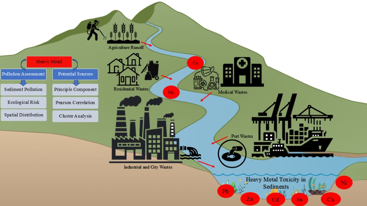
This study specifically aims to (i) evaluate the heavy metals (Cu, Ni, Zn, Pb, Mn, and Cd) concentration and the degree of heavy metals pollution by using pollution indices from the surface sediment samples in Malbasag river, (ii) determine the spatial distribution of HMs in the study area by using Arc GIS mapping and Inverse Distance Weighting (IDW) techniques, (iii) find out potential sources of heavy metals in sediment samples using multivariate statistical methods, (iv) evaluate the potential ecological risks posed by heavy metal contamination in the sediment samples and comparing the results with sediment quality guidelines (SQGs).
2. Materials and Methods
2.1. Study Area
The study was conducted on an important urban river that is found at the northwestern part of Leyte, Philippines. The Malbasag River is located in Ormoc City which is the second largest city in Leyte and has a total land area of 55, 774 hectares. The river is one of the two major drainages in the 4,567-hectare Ormoc Watershed and these rivers converge upstream of Ormoc City and the Isla Verde Area (Pearson and Oliver, 1992). The river is based in the city proper, directly connected with the Ormoc City Port and also 100 meters away from the City Bus Terminal. The port's key uses are for residential, commercial, industrial, and recreational activities. The Malbasag River is around 3 kilometers long, with a junction located 855 meters below the watershed's crest and 5 meters above average sea level (ASL). The river is a part of the government projects which is to guarantee a consistent water supply to 82 percent of the communities within the next 25 years (Tabios, 2020). The coordinates given are 11.04036° latitude and 124.63433° longitude. According to the 2020 census, the city mentioned in the text has a population of 230,998 inhabitants.
On November 5, 1991, Ormoc City experienced a deadly flood that claimed more than 6,000 lives. The Malbasag River was one of the rivers involved in the tragedy (Pearson and Oliver, 1992). The Philippine Bureau of Soils has designated the soils in the Ormoc Watershed as "upland soils." These soils are distinguished by their high potential for erosion and their unclear soil horizon. A high rate of soil formation is caused by the quick degradation of andesitic rock components and climate variables. Originally, soils were created from decomposed andesitic rocks (Pearson and Oliver, 1992). The Malbasag River drains the watershed's middle portion, which has just one subbasin. According to the Köppen-Geiger climate classification, the city's weather pattern falls within the tropical rainforest climate category (Af). The mean yearly temperature observed in Ormoc is recorded to be 26.1°C. The rainfall is around 2,216 mm per year. Precipitation is the lowest in April, with an average of 61 mm. The maximum quantity of rainfall is observed during the month of July, exhibiting an average value of 298 mm. Between the driest and wettest months, the difference in precipitation is 237 mm. The degree of fluctuation in the yearly temperature is approximately 2.1°C (WWF and BPI, 2013).
Port operations, residential garbage, commercial and industrial waste, and domestic raw sewage are all dumped into this river from nearby facilities. The river ecosystems have deteriorated alarmingly over the past few decades due to both natural and anthropogenic activity (Khan et al., 2023).
2.2. Sampling Sites
The sampling sites' locations are exhibited in Figure 1. Samples of surface sediment were taken at 10 Sites, namely Brgy. Donghol (S1), Brgy. Donghol(S2), Brgy. Patag(S3), Brgy. Patag(S4), Brgy. District 29 (Nadongholan)(S5), Brgy. District 29 (Nadongholan)(S6), Brgy North(S7), Brgy. East (S8), Brgy. East (S9), Brgy. South (S10) along the Malbasag River. Table 1 contains a brief summary of the sampling sites considered for this investigation.
2.3. Sample Collection
The Global Positioning System (GPS) device (Garmin, USA) was used to identify the sampling locations geographically. A total of thirty (30) sediment samples were collected during July, 2024. The sample collection day was very sunny and the average temperature in Ormoc City in July 2024 was approximately 31°C, with an average rainfall of 298 mm, typical for its wet season (Climate-Data, 2025). Ten different locations (S1–S10) were sampled from upstream to downstream of the river (Table 1). An Ekman grab sampler (7.5×3.2×3.1 cm) was used to collect sediment samples (top 2 cm of surface) from the river. To prevent cross-contamination and interference, the grab sampler was carefully cleaned repeatedly with deionized water after each sample collection. Approximately 750 g sediment was collected at each station. Following collection, sediment samples are stored in an icebox at 4°C, sealed in sterile zip-lock polyethylene bags, and sent to Visayas State University's Central Analytical Services Laboratory (CASL) in Baybay City, Leyte 6521, Philippines, for additional analysis.
2.4. Chemical Analysis
2.4.1. Reagents and Standards
Every reagent is Super pure or analytical grade (Merck, Darmstadt, Germany). All solutions were prepared using ultrapure water from a Milli-Q system (Millipore). Certified atomic absorption (AA) standard solutions with a concentration of 1000 mg/L for each element (Merck) were diluted to create calibration standards. Before being used, every glassware is thoroughly cleaned by rinsing it in deionized water after being soaked in diluted acid for at least 24 hours.
2.4.2. Analysis of Sediment Samples
The samples were oven dried at 45°C for 72 hours to gain constant weight, then stones and plant fragments removed physically. According to Islam et al. (2015), the dried samples are then pulverized with a mortar and pestle and sieved through a 2 mm aperture. The samples were kept in borosilicate sealed glass vials with labels prior to chemical properties evaluation. The modified USEPA Method 3050B (USEPA, 1996) was used to carry out the entire sediment digestion process in order to determine the heavy metal content. In brief, 2.0 g of each sediment sample is digested using concentrated 10 mL HNO3 (69%), 5 mL H2SO4 (98%), 5 mL HClO4 (70%) and 3 mL H2O2 (30%) in that good standing. After digestion, Whatman No. 41 filter paper (pre-washed with 0.1 M HNO3) was used to filter the solution, and the final volume was 100 mL of double-distilled water. The heavy metals in the samples were evaluated using flame AAS techniques using an atomic absorption spectrophotometer (AAS) (Model: Agilent 200, Series AA, Australia). The heavy metal concentrations and analytical parameters were measured using Atomic Absorption Spectroscopy (AAS).
2.5. Analytical Process for Physicochemical Parameter
The Physicochemical parameters included (pH, Electrical Conductivity, EC; % organic carbon, OC; % organic matter, OM; and % nitrogen, N) of the sediment’s samples were determined. The pH was determined using an OAKTON® pH 700 Benchtop pH meter. Coarse sediments and double-distilled water were combined in a 1:2.5 ratio, stirred violently, and allowed to stand for an hour. In order to determine the EC, coarse sediments and double-distilled water were combined in a 50 ml beaker at a 1:5 ratio, vigorously stirred, and allowed to stand for an hour. After this EC was determined by EC meter (OAKTON CTSTestr™, USA). Before use pH and EC meter in sediment sample analysis it was calibrated by standard solution. It was calibrated using pH values of 4.0, 7.0, and 10.0 as well as 1000 µs/cm for EC. Walkley and Black [38] measured OC and (OM) percentages using a spectrophotometric method at 627 nm. The calibration curve for organic carbon percentage showed a correlation coefficient of 0.991. The percentage OM was used conversion factor 2.0 and multiple with percentage of OC. Percentage of N was analyzed following Kjeldhal method manual titration procedure (Glazovskaya, 1991).
2.6. Quality Control
The quality of the analytical data was ensured through rigorous quality assurance and control measures, including adherence to standard operating procedures, calibration with standards, reagent blank analysis, and spiked replicate testing using AAS. The instrument was used three times to check for variances in the standard addition curve's slope using the standard references materials (SRMs) (R2> 0.991). The average measurements of heavy metals in the SRMs and the analytical conditions for AAS are provided in Table S3. The precision of the analytical results was confirmed by ensuring that the relative standard deviations (%RSD) across sample replicates remained below 10% (Table S1) (Rahman et al., 2022). The proportion of the experimental value to the certified value and the Z-score threshold (Bode, 1996; Rahman et al., 2018) were established to evaluate the accuracy and reliability of the laboratory results (Table S3). It is evident that the Z-scores for the reference materials range from 0.66 to 1.74 for all of the metals. The laboratory performance was seen as excellent based on the Z-score criterion (Z-score ≤ 2: satisfactory performance), and all of the elements' Z-score values fell within 2. Additionally, the relative error (RE%) for the metals under study was less than 10% (Table S3), demonstrating high agreement between measurement results and certified values. The ratio between experimental and verified values ranged between 0.93 and 1.14. The heavy metal measurement, and Statistical approach for AAS, in given the procedure that were used in AAS (Table S2). Each metal was analyzed twice, and the average of the outcomes was disclosed.
2.7. Sediment Quality Guidelines
According to MacDonald et al. (2000), sediment quality assessment guidelines (SQGs) are invaluable for screening sediment contamination by comparing the concentration of sediment contaminants with the appropriate quality guideline. These guidelines help interpret sediment quality by assessing potential impacts of sediment chemistry on aquatic life. They are useful for various purposes, such as designing monitoring programs, analyzing historical data, identifying the need for detailed sediment assessments, evaluating dredged material quality, conducting ecological risk studies, and setting remediation goals (MacDonald et al., 2000). SQGs such threshold effect level (TEL), probable effect level (PEL), effect range low (ERL), severe effect level (SEL), effects range medium (ERM), and lowest effect level (LEL) were utilized, however, to evaluate the possible biotic influence of metal(oid)s assessed in the sediment samples.
2.8. Pollution Assessment
The pollution indicators may play a part in the thorough evaluation of the level of soil pollution (Xu et al., 2008; Mazurek et al., 2017). A crucial factor in the interpretation of geochemical data is the selection of background values. Many researchers have utilized the average crustal abundance data or the average shale values as baselines for comparison (Covelli and Fontolan, 1997; Rubio et al., 2000; Sakan et al., 2009). The background values in this paper were used from pre-industrial global standard average shale values of heavy metals concentration, as there were no available data for the background concentrations of the Malbasag River sediments and soils of nearby places that were analyzed. This study employed four primary indices, enrichment factor (EF), geo-accumulation index (Igeo), pollution load index (PLI), and contamination factor (CF) to assess the degree of pollution in the sediment sample from the research region based on the concentrations of heavy metals.
2.8.1. Contamination Factor (CF)
The concentration of each metal in the sediment divided by the baseline or background value for the same metal provides the contamination factor (CF) (Hakanson, 1980).
CF values were interpreted as suggested by Hakanson (1980), where: CF < 1 indicates low contamination; 1 < CF < 3 is moderate contamination; 3 < CF < 6 is considerable contamination; and CF > 6 is very high contamination. The study obtained by using the standard pre industrial background value of metals (in mg/kg): 45 for Cu, 68 for Ni, 20 for Pb, 95 for Zn, 850 for Mn, 0.3 for Cd (Turekian and Wedephol, 1961; Hakanson, 1980).
2.8.2. Pollution Load Index (PLI)
PLI is an integrated method for evaluating the quality of sediment. The geometric mean of the metal’s contamination factor is known as the PLI. The PLI of the site was calculated by taking the n root of the contamination factor derived from all metals (Tomlinson et al., 1980). The PLI was designed by Tomilson et al. (1980) and is shown below:
An easy way to compare levels of heavy metal pollution is to use this empirical indicator. PLI > 1 indicates the presence of pollution; PLI < 1 indicates the absence of metal contamination (Tomlinson et al., 1980).
2.8.3. Geo Accumulation Index (Igeo)
Metal contamination in soils and aquatic sediments is measured using the geoaccumulation index (Igeo). The following formula defines the geo accumulation index (Igeo):
where Bn is the metal’s geochemical background concentration of element (Muller, 1969) and Cn is the concentration of metals analyzed in sediment sample concentrations (n). The background matrix adjustment factor because of the lithospheric effects is 1.5. There are seven classes in the geo accumulation index (Muller, 1969) . Igeo ≤ 0 for Class 0 (practically unpolluted); 0 < Igeo < 1 for Class 1 (unpolluted to moderately polluted); 1 < Igeo < 2 for Class 2 (moderately polluted); 2 < Igeo < 3 for Class 3 (moderately to heavily polluted); 3 <Igeo <4 for class 4 (heavily polluted); 4 < Igeo < 5 for Class 5 (heavily to extremely polluted); 5 > Igeo for class 6 (extreamly polluted) (Bhuyan et al., 2010).
2.8.4. Enrichment Factor (EF)
The enrichment factor (EF) is a useful tool for determining the extent of anthropogenic HMs contamination (Maison, 1966; Sakan et al., 2009). The following relationship is used to calculate the EF:
Iron (Fe) used as the reference element for geochemical normalization in the present study for an array of reasons, including the fact that it is associated with solid surfaces, that its geochemistry is similar to that of many trace metals, and that its natural concentration tends to be uniform (Bhuyan et al., 2010). For the EF calculation, the background metal concentrations were 20 for Pb, 50 for Ni, 68 for Zn, 600 for Mn, 0.1 for Cd, and 25 for Cu (Maison, 1966; Atgin et al., 2000). The EF values were interpreted according to the guidelines proposed by Sakan et al. (2009), where EF < 1 denotes no enrichment, 3–5 moderate enrichment, 5–10 moderately severe enrichment, 10–25 severe enrichment, 25–50 very severe enrichment, and >50 extremely severe enrichment.
2.9. Potential Ecological Risk Index (RI)
Since heavy metal concentrations in sediments are increasing and can be harmful to ecological health when released into water, evaluating the possible ecological risk of heavy metal contamination was suggested as a helpful technique for water pollution mitigation (Hu et al., 2019). In order to determine which lakes, rivers, and chemicals require special attention, Hakanson (1980) devised a system to evaluate the prospective ecological risk index for aquatic pollution management reasons. Using this approach, the following formulas may be used to calculate the potential ecological risk factor (Eir) of a single element and the potential ecological risk index (RI) of a multi-element (Rahman et al., 2014):
Where, Tri is the toxic response factor for the specified element of "i" which takes into consideration both the sensitivity and the toxic requirements; and CFi is the contamination factor for the element of "i". The toxic response factors for Pb, Ni, Cu, Mn, Cd and Mn were 5, 6, 5, 1, 30 and 1 respectively (Hakanson, 1980; Taylor and McLennan, 1985). The possible ecological risk assessment was calculated using equations 1, 4, and 5.
2.10. Toxic Units
To compare the relative impacts, the toxicities of different heavy metals were normalized using toxic units (TUs) (Bai et al., 2011b). According to Pedersen et al. (1998), TUs are the ratios of the observed levels of each heavy metal to the probable effect level (PEL) values. Equation (7) was used to get the TU for each heavy metal.
where PELi is the investigated heavy metal of ith parameter associated value and Ci is the analyzed heavy metal concentration of ith parameter in sediment. According to MacDonald et al. (2000), these values are shown as Ni = 36, Pb = 91, Cd = 3.5, Cr = 90, Cu = 197, and Zn = 315. The toxic unit total (∑TU) was computed using equation (8).
where ∑TU is the total of all heavy metals' toxic units.
2.11. Toxic Risk Index (TRI)
The ecotoxicity may be underestimated by the toxic units (TUs) since the TEL effects are not taken into account. Zhang et al. (2017) developed a toxic risk index, which was used to give a more thorough assessment of the biota's hazards in the aquatic environment. TRI was computed using Eq. (9) using two threshold values for SQGs (TEL and PEL standard).
PEL and TEL stand for the probable impact level and threshold effect level for the ith metals, respectively, whereas Ci indicates the concentration of the ith metal. As shown in Table 3, TEL and PEL standard values from MacDonland et al. (2000) were used in this study. The following is an interpretation of the TRI values: 'TRI ≤ 5' denotes no toxic risk, '5 < TRI ≤ 10' denotes low toxic risk, '10 < TRI ≤ 15' denotes moderate toxic risk, '15 < TRI ≤ 20' denotes major hazardous danger, and 'TRI > 20' denotes extremely high toxic risk.
2.12. Modified Hazard Quotient (mHQ)
Based on the severity of heavy metal contamination, a new index is created and proposed in this study to evaluate sediment pollution. Through comparison of the metal content in sediment with the synoptic metal concentration, this unique technique allows contamination evaluation. According to earlier descriptions (Benson et al., 2018; MacDonald et al., 2000), the distributions of adverse ecological effects for three somewhat varied threshold values (TEL, PEL, and SEL). The following method may be used to calculate the metals' modified hazard quotient (mHQ), which is a crucial assessment tool that clarifies the level of danger that each heavy metal poses to the aquatic environment and biota.
Threshold effect level, probable impact level, and severe effect level are denoted by the abbreviations TELi, PELi, and SELi for each metal. The detected concentrations of heavy metals in the sediment samples are denoted by Ci. For mathematical and ranking purposes, the square root is employed as a drawdown function in the equation. The Modified Hazard Quotient is categorized as follows: mHQ > 3.5 indicates extreme contamination severity; 3.0 ≤ mHQ < 3.5 indicates very high contamination severity; 2.5 ≤ mHQ < 3.0 indicates high contamination severity; 2.0 ≤ mHQ < 2.5 indicates significant contamination; 1.5 ≤ mHQ < 2.0 indicates moderate contamination; 1.0 ≤ mHQ < 1.5 indicates low contamination severity; 0.5 ≤ mHQ < 1.0 indicates very low contamination severity; mHQ < 0.5 indicates nil to very low contamination severity (Benson et al., 2018; MacDonald et al., 2000)
2.13. Linear Regression Model Analysis
One method for examining how one variable (referred to as the dependent variable) is influenced by one or more independent variables (referred to as the explanatory variables) is regression analysis. Regression analysis allows for the functional expression of the relationship between the explanatory and dependent variables (Chen et al., 2021).
Y = β0 + β1X1a + ……+ βk Xka + ϵa
Where a = 1, 2, 3, n, ε is the random error term, β0 is the y-intercept, β1 is the slope of the regression line, X is the predictor, and Y is the dependent variable. In our study, we applied this model to identify the linear relationship of a set of independent variables (such as HMs) with the dependent variable (e.g., ecological risks indices).
2.14. Statistical Analyses
The data was statistically performed using R (V. 4.4.2), Arc GIS (V. 10.5), and Microsoft Excel-2021 software. To investigate the significant temporal and spatial differences, a one-way nested analysis of variance (ANOVA) was conducted at a 95% confidence level (p < 0 '***' 0.001 '**' 0.01 '*' 0.05 '.' 0.1'' 1). The data was summarized using ranges, median values, percentages of relative standard deviation (%RSD), mean values, and standard deviations (Std). A systematic technique for measuring a probability or frequency distribution is the coefficient of variation (% CV). In this study determined the CV value for understanding the stability of data. The geographical distribution of heavy metals in the study areas calculated using the inverse distance weighting (IDW) method in Arc GIS software (V. 10.5). The IDW method was chosen for its ability to provide spatially interpolated values with high speed and accuracy. Pearson's correlation matrix (PCM), principal component analysis (PCA), and cluster analysis (CA) are multivariate statistical techniques used to determine the geochemical process and the probable origins of heavy metals in sediments when taking into account the p value < (0 '***' 0.001 '**' 0.01 '*' 0.05 '.' 0.1 '' 1). The PCA with varimax rotation was performed to enhance the interpretability of the factors without altering the original sediment dataset. This approach grouped variables based on their specific properties. Varimax rotation effectively minimizes the influence of less significant variables in the PCA dataset. The study results are explained using PCA using the mean value of each variable, with an eigenvalue >1 and a loading value > 0.7 for each of the main components from the analysis table. Moreover, the cluster analysis was performed to determine the similar groups based on their similar characteristics within the class and dissimilar characteristics among the other classes. In this study, to determine the relationship dependable variable (RI) and predictor (metals), stepwise linear regression analysis was undertaken. Correlation analysis was carried to discarded the number of explanatory variables (Pb, Zn) and decrease the collinearity in linear regression model. The regression model may have been overfitted because of the small sample size, which can reduce the reliability of the results and limit their applicability to other similar situations or locations.
3. Results and Discussion
3.1. The Physicochemical Properties of Sediment Samples in the Study Area
A river basin's physicochemical characteristics and heavy metals are influenced by variations in topography and hydrogeology. Furthermore, even over short distances, variations in local temperature, salinity, rainfall, land runoff, anthropogenic activities and geomorphological configuration are important factors in the fluctuation of heavy metals between catchment areas (Costa et al. 2001, Wang and Qin 2006). In Table 2, the physicochemical properties of sediments are displayed.
The study area’s pH ranged from 5.29 to 6.59 with average value of 5.93 ± 0.323 which meant that the sediments were moderately acidic. The EC values in the sediments varied from 4.34 to 1700.0 µS/cm, with average value of 278.56 ± 467.33 µS/cm. The organic carbon (OC) in the study Sites ranged from 0.210 to 1.501 percentages and the average value was 0.736 ± 0.408 percentage. The differences in the EC values and organic carbon were due to discharging waste from residential and commercial areas, agricultural runoff, vegetation, salinity, and industrial sewage from the port area. Moreover, the percentage of nitrogen in the study Sites varied from 0.011 to 0.267 and the average value was 0.112 ± 0.081 %. The physicochemical parameters of sediments at different sampling locations have percentages of relative standard deviation (%RSD) ranging from 5.44 to 167.752. The %RSD for each sampling point is shown in the supplementary section (Table S1) and the ANOVA test at 95% confidence interval indicated the significant differences in all physicochemical properties across the Sites (p<0.001 for most properties) that can be found in the supplementary section (Table S4). These opinions imply that Site specific factors (vegetation, industry, port activities, agricultural farm) contribute to the variability in sediments properties in the river.
3.2. Heavy Metal Concentration
Urban and port effluents have been recognized as one of the main environmental hazards. As a result, sediment samples from the Malbasag River that are directly connected to the port (Ormoc City Port) were examined in order to ascertain the heavy metal concentration, which is shown in Table 3. According to the average data analysis, the Malbasag River's sediment has the following total heavy metal accumulation order (mg/kg as dry weight basis): Mn > Zn > Cu > Ni > Pb > Cd. The concentrations of the heavy metals (Cu, Ni, Pb, Zn, Mn, and Cd) for each sampling point are listed in the supplementary section (Table S1). According to the data, Cd was only slightly deposited in the sediments, whereas Mn was extremely concentrated (Figure 2). The percentage of relative standard deviation (%RSD) for the studied heavy metals distribution in sediments at various sampling points showed that the abundance of Cu, Ni, Pb, Zn, Mn, and Cd varied widely (%RSD: 9.38–81.17%) in Table 3, and the ANOVA test at a 95% confidence interval and p value (0 '***' 0.001 '**' 0.01 '*' 0.05 '.' 0.1'' 1) indicated that most of the metals were highly significant among their Sites. The ANOVA result in this investigation showed that there was spatial heterogeneity in the concentrations of heavy metals (Cu, Ni, Pb, Zn, and Cd) and that these variations were very significant (P<0.001) among the Sites (Table S5). It’s mentioned that specific Sites are might be affected by anthropogenic source (agricultural runoff, domestic and urban waste, port activities, onloading fishing boat, hospital and medical wastewater discharge). On the other hand, the metal Mn concentrations showed insignificance (p = 0.076) with the Sites, indicated that possible affected by natural geochemical and climatic factors.
Table S1 shows that heavy metal concentrations at Sites (Sites 6 - Site 10) were much higher than at other Sites due to their location downstream of the river and considerable discharge of urban and port materials waste. The highest concentrations of heavy metals were observed at Site-10 (Brgy South). These elevated levels are likely attributed to port activities and untreated waste discharges directly from the Ormoc City port, the city bus terminal, and the food park in the Township area. Site-9 (Brgy East) which receives untreated medical and domestic waste from the urban area, Site-8 (Brgy East) which receives waste water drains that mixed partially treated domestic and industrial waste water from Brgy East that situated in the main township. Also, Site 8-10 easily receive pollution from the port because of the high tide. Site-7 (Brgy North) which receives agricultural runoff from rice fields and Pura Agriventures and Development Corporation (PADC) farm untreated waste, waste water from Brgy 29, in Ormoc City. Site -6 (Nadongholan) receive pollution from big agricultural field and residential area from the Township. The lowest polluted Site was estimated at Site -4 (Brgy Patag) where established water treatment plant and this plant supply water for whole City communities. The plant maintained well treatment process before discharge the waste from the plant. According to Table S1, the total metal concentrations in this investigation were as follows: Site-10 > Site-9 > Site-7 > Site-6 > Site-8 > Site -1 > Site-3 > Site-2 > Site-5 > Site-4. As a result, it has been reported that the origins of these metals in sediments were primarily anthropogenic (Rahman et al., 2019), and the examined heavy metals were dispersed uniformly. The sediment quality guidelines (SQGs) threshold values-Probable Effect Level (PEL), Threshold Effect Level (TEL), Severe Effect Level (SEL), Effect Range Low (ERL), Lowest Effect Level (LEL), and Effects Range Medium (ERM) were also compared with the concentrations of the heavy metals under investigation (mg/kg) in the sediment samples.

Table 3.
Concentration of heavy metals in sediment samples from Malbasag River, Leyte, Philippines.
| Concentration (mg/kg) as dry weight basis | ||||||
|---|---|---|---|---|---|---|
| Cu | Ni | Pb | Zn | Mn | Cd | |
| Experimental Data | ||||||
| Mean (n = 30) | 52.516 | 33.058 | 21.955 | 54.643 | 141.096 | 0.801 |
| Std | 13.468 | 22.833 | 7.984 | 28.820 | 13.239 | 0.650 |
| RSD (%) | 25.646 | 69.069 | 36.366 | 52.742 | 9.383 | 81.170 |
| Median | 50.164 | 22.680 | 20.790 | 42.724 | 142.746 | 0.810 |
| Min. | 32.568 | 11.760 | 12.915 | 27.459 | 100.502 | 0.014 |
| Max. | 74.865 | 81.480 | 42.350 | 105.391 | 165.984 | 2.014 |
| SQG Threshold values | ||||||
| LEL (Persuad et al., 1993) | 16.0 | 16 | 31.0 | 120 | 460 | 0.6 |
| SEL (Persuad et al., 1993) | 110 | 75 | 250 | 820 | 1100 | 10.0 |
| TEL (MacDonald et al., 2000) | 35.7 | 18 | 35 | 123 | - | 0.59 |
| PEL (MacDonald et al., 2000) | 197 | 36 | 91 | 315 | - | 3.5 |
| ERL (Long et al., 19950) | 34 | 20.9 | 46.7 | 120 | - | 1.2 |
| ERM (Long et al., 19950) | 270 | 51.6 | 218 | 410 | - | 9.6 |
| TRV (USEPA, 1999) | 16.0 | 16 | 31 | 110 | - | 0.6 |
| Impact (%) on ecology | ||||||
| <LEL | - | 30.0 | 90.0 | 100 | 100 | 40.0 |
| LEL-SEL | 100 | 70.0 | 10.0 | - | - | 60.0 |
| >SEL | - | - | - | - | - | - |
| <TEL | 10.0 | 43.3 | 90.0 | 100 | - | 40.0 |
| TEL-PEL | 90.0 | 26.7 | - | - | - | 60.0 |
| >PEL | - | 30.0 | - | - | - | - |
| <ERL | 6.76 | 53.3 | 100 | 100 | - | 80.0 |
| ERL-ERM | 93.3 | 20.0 | - | - | - | 20.0 |
| >ERM | - | 30.0 | - | - | - | - |
3.2.1. Copper (Cu)
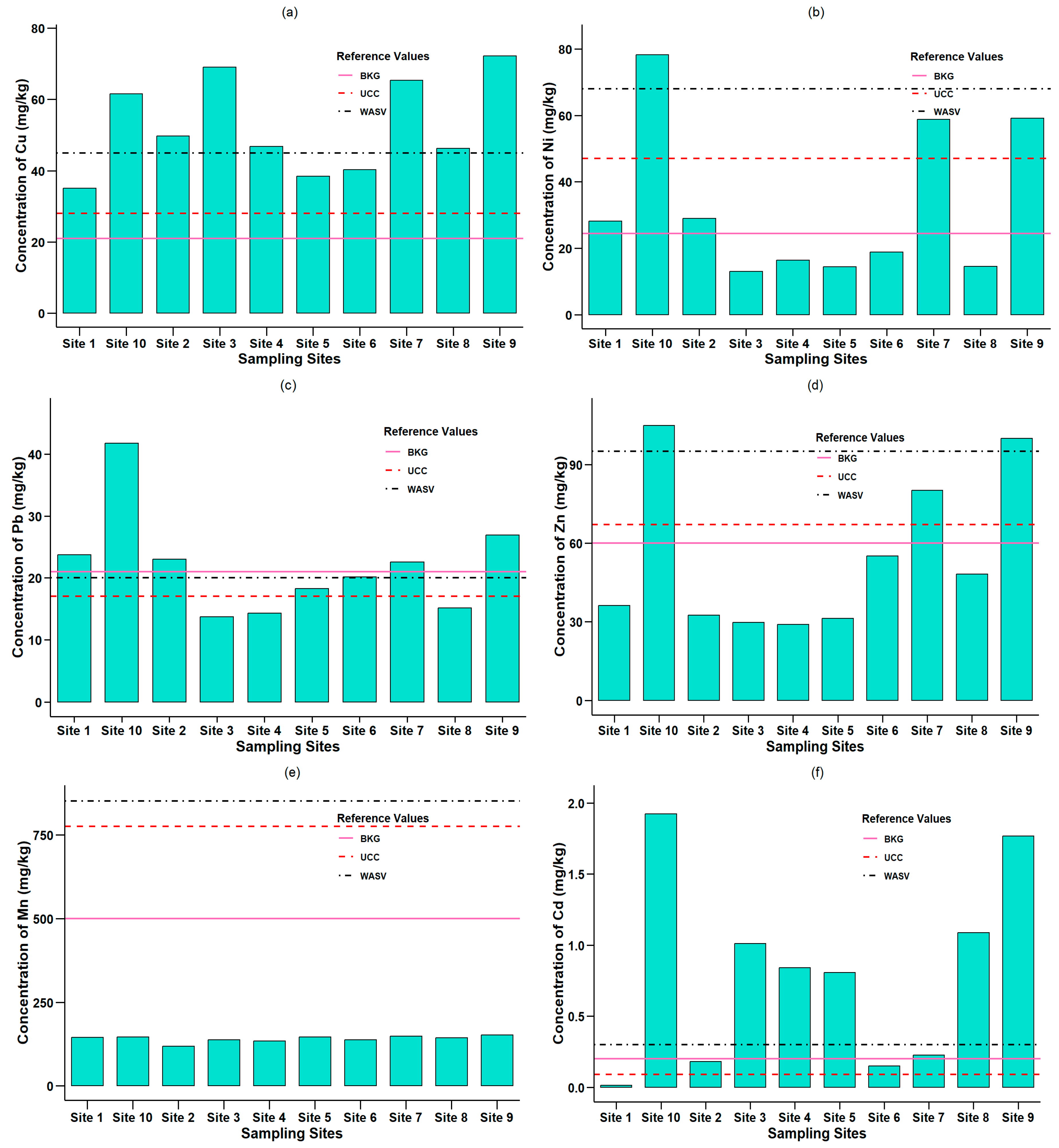
The investigated area's sediment samples had an average Cu concentration of 52.5 ± 13.4 mg/kg, with a range of 32.56 to 74.86 mg/kg (Table 3). The average Cu concentration in the sediment samples in the study area was found to be higher than the background value of soils (UNEP, 1990) (25 mg/kg), the average sediment value (50 mg/kg) (Turekian and Wedephol, 1961), and the upper continental crust value (28 mg/kg) (Rudnick and Gao, 2014) (Figure 2a). However, the coefficient of variance for Mn concentration across sampling points showed moderate variability (25.64 % < CV ≤ 50) (Zhang et al., 2010), suggesting that the research area's Cu sources could be mostly natural and anthropogenic (Table S5). The range of Cu concentration in the sediment samples was then found to be lower than that of several different river sediments in the Philippines, including Manila Bay (Suthar et al., 2009) and the Mangonbangon River (Pacle et al., 2018); additionally, it was higher than the results of river sediments in several other countries around the world (Sany et al., 2013; Hanif et al., 2016; Lundy et al., 2017) (Table S6). However, the high Cu copper content was Site 9 and 10 (Brgy East and South). Notably, Cu is typically released into the environment through car exhausts, smelting from coal burning furnaces, and other sources (Xia and Gao, 2011; Rahman et al., 2022). Due to the study sites' accessibility to ports, major towns, road dust, fishing boats, and urban areas, there may be a source of copper contamination in the sediment samples. It was found that the average concentration of copper in sediment samples above all of the SQG threshold values (LEL, SEL, TEF, PEL, ERL, ERM, and TRV (Persuad et al., 1993; Long et al., 1995; USEPA, 1999). It was observed that 30%, 10%, and 6.76% samples were classified as less than LEL, TEL, and ERL, respectively, whereas 100%, 90%, and 93.3% of samples fell into the LEL-SEL, TEL-PEL, and ERL-ERM categories. This element is essential for plant growth because it is found in many enzymes and proteins (Loksa et al., 2004). Cu is frequently used in electrical wire, roofing, alloys, pigments, culinary utensils, and pipelines (Pandy and Singh, 2015).
3.2.2. Nickel (Ni)
The sediment samples had an average Ni concentration of 33.0 ± 22.8 mg/kg, with a range of 11.7 to 82.4 mg/kg (Table 3). Site-10> Site-9> Site-7> Site 2> Site-1> Site-6> Site-4> Site-5> Site-8> Site-3 was the descending order of variability for the Ni concentration in the study sites (Figure 2b). Ni usually exists in soil in the organically bound form, which enhances its mobility and bioavailability in neutral and acidic environments (Loska et al., 2004). In sediment samples Site-1 (Brgy Donghol), Site-2 (Brgy Donghol), Site-7 (Brgy Norh), Site-9 (Brgy East), Site-10 (Brgy North) showed above the background values (24.5 mg/kg) (UNEP, 1992). Site-7, Site-9, and Site-10 was found higher than upper continental crust (Rudnick and Gao, 2014) value (47 mg/kg). Site 10 the Ni concentration showed above than average shale (Turekian and wedephol, 1961) value (68 mg/kg). However, the elevated Ni concentrations in Sites 9 and 10 (59.0 and 78.1 mg/kg) suggest a higher input, which could originate from urban waste, oil and gas refinery machinery and equipment, wood chips and preservative chemicals at the port, untreated hospital wastewater, household sludge, and agricultural runoff from sugarcane and pineapple fields. However, the Pb concentration's coefficient of variation (CV) varied greatly across sampling points (69.06% < CV ≤ 100) (Zhang et al., 2010), suggesting that the research area's Ni sources may be predominantly human disturbances. Also, in this study showed the ranged of Ni concentration higher than other Philippine’s River sediments samples (Suthar et al 2009). The Ni concentration in sediments also comparison with other international river sediments samples study and revealed that the study sediments less than several international rivers: Bangladesh (Islam et al., 2015), Turkey (Varol, 2011) (Table S6). The average Ni concentration in sediments were compared with sediments quality guideline values (LEL, SEL, TEF, PEL, ERL, ERM and TRV). It observed that 30%, 43.3%, 53.3% samples are less than LEL< TEL, and ERL and 30% sediments sample higher than ERM value. Additionally, Table 3 shows that 70%, 26.7%, and 20% of the samples were classified as LEL-SEL, TEL-PEL, and ERL-ERM, respectively. The findings show a negative impact on bottom-dwelling creatures, which were expected to occur regularly (Varol, 2011).
3.2.3. Lead (Pb)
The ecology may be seriously threatened by Pb due to its extremely dangerous toxicity level, even at low concentrations (Patra et al., 2011). Following a sequence of Site 10 > Site 9 > Site 1 > Site 7 > Site 2 > Site 6 > Site 5 > Site 8 > Site 4 > Site 3 (Figure 2c), the average Pb concentration wad found 21.95 ± 7.98, ranging from 12.9 to 42.3 mg/kg (Table 3). Interestingly, there was no downstream trend in the declining order of heavy metals in the studied sites. This is likely because of the influence of mineralogical composition, source variability, and the dominance of physicochemical processes like organic matter variation, adsorption, absorption, precipitation, redox reactions, and rocks. In this study area Pb concentration cross the upper continental crust value (17.0 mg/kg) except Site-3 (Brgy Patag), Site-4 (Brgy Patag), and Sit-8 (Brgy East) (Figure 2c). The coefficient of variance for Pb concentration in various sampling points showed moderate (36.36% < CV ≤ 50) variability (Zhang et al., 2010), suggesting that the sources of Pb in the study area may be influenced by both natural and man-made sources. Site-9 (Bgy East) and Site-10 (Brgy South) were established close to the city center and port area. Although the Pb concentration in the study area was higher than in some international river sediments, such as Pakistan (Hanif et al., 2016) and Italy (Lundy et al., 2017), the ranged Pb level was found to be lower than the value observed in national river sediments: Pasig, Marikana (Suthar et al., 2009), and Mangobangon (Pacle et al., 2018) (Table S6). However, the 10% Pb concentration value fell between the LEL and SEL categories, although the average Pb content for 90%, 90%, and 100% sediment samples was determined to be below the severe effect level (SEL), threshold effect level (TEL), and effect range low (ERL) values (Table 3). Thus, similar to other basic divalent metals (Mn2+ and Zn2+), Pb2+ may have altered the osmotic balance of bacterial cells, the compliance of proteins and nucleic acids, and the inhibition of bacterial chemical movement (Fashola et al., 2016). These changes may have an effect on ecology (Rahman et al., 2014).
3.2.4. Zinc (Zn)
The sediment sample's average Zn content was 54.6 ± 28.8 mg/kg, with a range of 27.4 to 105.3 mg/kg (Table 3). Site-4 (Brgy Patag) had the lowest Zn content, whereas Site-10 (Brgy South) had the highest. In this study showed that 3 Sites are more polluted same as Ni concentration. Site-7, Site-9 and Site-10 revealed the average concentration of Zn higher than the background value (UNEP, 1992) and upper continental crust value (Rudnick and Gao, 2014). Zn concentrations at Sites 9 and 10 were greater than the global average (Turekian and Wedephol, 1961) (Figure 2d). Vehicle emissions as well as commercial and industrial discharge might be responsible for the higher content of Zn in the sediments (Sekabira et al., 2010; Islam et al., 2015). In addition, Sites 10, 9, and 7 in this study are the points of entry for metals into the Port, and the excessive land use for urbanization, industrialization, and economics (such as manufacturing, plantations, and animal farming) that takes place in this area of the rivers has an effect on the metals carried out at the downstream Sites. Furthermore, the average Zn concentration in the sediment samples was found to be lower than that of several different river sediments in the Philippines, , including Manila Bay (Suthar et al., 2009) and the Mangonbangon River (Pacle et al., 2018); it was also higher than the results of river sediments in a number of other countries, including Italy (Lundy et al., 2017), Pakistan (Hanif et al., 2016), and Malaysia (Sany et al., 2012) (Table S6). According to sediment quality guidelines (SQGs) the average Zn concentration in all sediments sample in this study area observed lower than LEL, TEL, and ERL threshold level. Which is indicated the toxicity is negligible and functioning good environment for aquatic ecology.
3.2.5. Manganese (Mn)
This investigation showed that the sediment samples had an average Mn content of 141.0 ± 13.2 mg/kg (Table 3). The sample point of Site-2 (Brgy Donghol) had the lowest Mn concentration, whereas the sampling point of Site-9 (Brgy East) had the highest Mn concentration. The following order was determined for the average Mn concentration in the sediment samples taken from the various sampling locations: Site-9> Site-7> Site-10> Site-5 > Site-1 > Site-8 > Site-3 > Site-4> Site-2, correspondingly (Figure 2e). According to the following order, the areas with the highest levels of Mn pollution were lower stream and close to the port, while the study area's Mn concentration showed low variability (9.38% < CV ≤ 10) across sample locations (Zhang et al., 2010). It suggests that natural sources and site-specific elements including rainfall, soil erosion, and andesite rock formations may be the primary sources of Mn in the research region. On the other hand, the average Mn concentration was found to be much lower than the global average soil value (Turekian and Wedephol, 1961), the upper continental crust value (Rudnik and Gao, 2014), and the background value of soils (UNEP, 1992). According to Suthar et al. (2009), Pacle et al. (2018), and Varol (2011), the average Mn content was subsequently lower than the sediment values reported by national and international scientists worldwide (Table S6). According to Table 3, the average Mn content in all of the sediment samples used in this investigation was found to be below the LEL and SEL threshold values (Persuad et al., 1993). This suggested that there was less Mn pollution in the research area.
3.2.6. Cadmium (Cd)
The average Cd concentration in this investigation was 0.80 ± 0.65 mg/kg, with a range of 0.01 to 2.014 mg/kg (Table 3). Site-10> Site-9> Site-8> Site-3> Site-4> Site-5> Site-7> Site-2> Site-6> Site-1 was the decreasing order of the average Cd content in the sediments sample. This investigation found that the Cd content was higher than the top continental crust (Rudnick and Gao, 2014) (0.09 mg/kg), soil background (0.2 mg/kg) according to UNEP (1992), and world average shale (Turekian and Wedephol, 1961) value (0.3 mg/kg) (Figure 2). The highest Cd concentrations were found downstream of the river (Sites 8 to 10), which are directly connected to port activities, hospitals, city bus terminals, shipping boats, repair and painting ships, domestic and industrial drainage, and the discharge of untreated or slightly treated wastewater. Furthermore, as Cd is typically found in phosphorus fertilizer and animal dung, storm water runoff from agricultural regions may further contribute to metal contamination (Watanabe et al. 1996). According to Zhang et al. (2010) the statistical analysis of the average values in several sample points showed very significant (CV <100) variability, suggesting that the study area's Cd sources may be mostly anthropogenic. The varied Cd concentrations of sediment samples from rivers in the Philippines and other countries were compared in this study. It was noted that the reported values for the Cd content were lower than those of many different countries, including China (Yuan et al., 2014), Turkey (Varol, 2011), and India (Pandy et al., 2015a) but it crossed some of the international river such as Poland (Obolewski and Glinska-Lewezuk, 2013), Malaysia (Sany et al., 2013) (Table S6). Additionally, this study compared the Cd content in evaluated sediment samples with the threshold values for SQGs (LEL, TEL, SEL, PEL, ERL, and ERM). It was found that 60%, 60%, and 20% of the sediment samples fell into the LEL-SEL, TEL-PEL, and ERL-ERM categories, respectively, whereas 40%, 60%, and 80% less than LEL, TEL, and ERL (Table 3). It could be suggested localized moderate to high ecological risks. This includes the potential for bioaccumulation, sublethal toxicity, and disruptions in sediment-associated biodiversity and ecosystem services (Long and Morgan, 1990).
Figure 2.
Concentration (mg/kg) of heavy metals (a) Cu, (b) Ni, (c) Pb, (d) Zn, (e) Mn, and (f) Cd in sediment samples from the study area compared to the suggested levels levels (Turekin and Wederpohl, 1961; CNEMC, 1990; Rudnick and Gao, 2014). NB. WASL stands for world average soil values (Turekin and Wederpohl, 1961), BKG for background soil values (CNEMC, 1990), and UCC for upper continental crust values (Rudnick and Gao, 2014).
3.3. Geochemical Indicators of Contaminated Sediments
3.3.1. Contamination Factor (CF), Pollution Load Index (PLI), Geo-Accumulation Index (Igeo), and Enrichment Factor (EF)
Two significant indices were introduced by Hakanson (1980) for calculating the metal pollution in sediment: the pollution load index (PLI) and the contamination factor (CF). However, many scientists have utilized such indicators significantly to assess the level of heavy metal contamination in sediment samples (Tomlinson et al., 1980; Saha et al., 2016). The outcomes for the pollution load index (PLI) and contamination factors (CFs) are showed in Table S7. The greatest CF values for all metals investigated were discovered at Site-10 (Brgy South) and Site-9 (Brgy East), which receive a significant volume of waste from port activities, hospitals, and the urban wastewater drainage system. Total CF was distributed as follows: Site-10, Site-9, Site-7, Site-8, Site-4, Site-3, Site-2, Site-5, Site-6, and Site-1. The Site-7 that receive storm water runoff from agricultural areas, animal farming waste from Brgy, District 29, Ormoc City. While Cu, Pb, and Fe exhibited extremely high levels of contamination (CF > 6), the contamination factor (CF) value for other metals indicated a moderate level of contamination (CF > 1) (Figure 3). Cu > Pb > Fe > Zn > Cd > Mn was the overall declining order of the CF for all metals.
The degree of heavy metal contamination in the specific site under this study was determined using the pollutant load index (PLI) (Tomlinson et al., 1980; Brady et al., 2015). This index is an easy method to compare the pollution levels of various locations. The mean value of the pollutant load index (PLI) was 0.66, while the range was 0.35 to 1.19 (Table S7). The mean value conforming that the river is low contamination (PLI<1). However, higher PLI value was found in Site-9 (Brgy East) and Site-10 (Brgy North) that indicated the sediments in this Site were polluted (PLI>1). Other all Sites PLI value was found less than one (Figure 4) that indicating the Sites sediments were pollution free. In this study revealed that Cu, Pb, and Cd is the major contributor for sediment pollution. Site-10 > Site-9 > Site-7 > Site-8 > Site-4 > Site-3 > Site-2> Site-5> Site-6> Site-1 was the decreasing Site order that the PLI followed to (Figure 4). The residents can gain some insight into the environmental quality through the PLI.
In order to determine the degree of heavy metal contamination in sediment samples, this study makes significant use of the geo-accumulation index (Igeo), which has been widely used in European trace metal investigations since the late 1960s (Muller, 1969). The ranged of Igeo values for different sediment samples were found to be -0.95 to 0.10, −2.96 to −0.38, −1.13 to 0.48, -2.10 to -0.82, -2.29 to -0.44, -3.43 to -3.06, -1.52 to 5.41 for Cu, Ni, Pb, Fe, Zn, Mn, and Cd respectively (Figure 5). Each metal and each sampling point's comprehensive data are included in the supplemental section (Table S8). The Igeo values of the heavy metals under study are displayed in Figure 5. In Site-3 (Brgy Patag) and Site-9 (Brgy East), the Igeo for Cu was 0.03 and 0.10, respectively, according to this analysis, indicating that both samples are class 1. Site-9, Igeo for Pb was individually 0.48 that’s means it fallen into class 1 or unpolluted to moderately polluted. The other Igeo for Cu, Ni, Pb, Fe, Zn, and Mn were less than zero which indicated the sediments was not polluted. The Igeo for Cd in the study area mean concentration of 3.28 (Table S8). The maximal positive values of Cd are shown in Figure 5. However, the Igeo values for Cd in 10%, 10%, 20%, 40%, and 20% of the sampling points fall into class 0, class 2, class 3, class 5, and class 6, indicating that the sediments are respectively uncontaminated, moderately contaminated, moderately to heavily contaminated, heavily to extremely contaminated, and extremely contaminated (Muller, 1969). The Igeo values for the heavy metals under study were arranged in the following decreasing sequence, in Figure 5: Cd > Pb > Zn > Cu > Fe > Ni > Mn.
According to Zhang and Liu (2000), the metal is entirely produced from natural processes or crustal materials if the EF value is between 0.05 and 1.5. However, if the EF value is larger than 1.5, the sources are more likely to be human-made. In the sediments of the Malbasag River, the mean EF values for every metal examined in this study-aside from Mn-were >1.5, suggesting that human activity has an effect on the metal levels in the river (Figure 6). The EF value for Cu, Cd in the sediments of Site-3 was 7.87, and 28.78, showing “severe” and “very severe enrichment” that indicating highly anthropogenic activities, mainly this Site located the livestock farm, residential, and agricultural area. Moreover, most of the Sites the highest EF values were found at Site-9 (Brgy East), and Site-10 (Brgy South) due to industrialization, urbanization, slightly treated drainage wastewater, deposition of port and medical untreated waste from Ormoc Township. Total EF values followed the order of Site-3 > Site-9 > Site-10 > Site-5 > Site-4 > Site-8 > Site-7 > Site-6 > Site-2 > Site-1 (Figure 6).
3.4. Ecological Risk
The results of the evaluation for the potential ecological risk index (RI) and the prospective ecological risk factor (Eri) are shown in Table 4. Cu, Ni, Pb, Zn, Mn, and Cd were found to have possible ecological risk factors (Eir) ranging from 3.89 to 8.01, 1.15 to 6.89, 3.42 to 10.43, 0.30 to 1.10, 0.13 to 0.17, and 1.5 to 192, respectively, with average values of 5.82, 2.91, 5.48, 0.57, 0.16, and 80.12. According to Table 4, the possible ecological risk factors for heavy metals in the Malbasag River sediments were as follows: Cd > Pb > Cu > Ni > Zn > Mn.
Cd presented a moderate to significant ecological danger, with a mean value of 95.10 (Table 4). Cd may have been present in the sediments as a result of agricultural runoff into the river and the release of waste and oily effluents from port activities. Other heavy metal studies' Eri results (Cu, Ni, Pb, Zn, and Mn) indicate minimal ecological risk due to a lower toxic response factor (Tri). The potential ecological risk index for the heavy metal according to study in the sediments of the Malbasag River was found to be in the following order: Site-10 > Site-9 > Site-8 > Site-3 > Site-4 > Site-5 > Site-7 > Site-2 > Site-6 > Site-1. The RI values at the sampling sites, however, varied from 14.42 to 217.72, suggesting that all of the sampling sites had moderate to significant ecological risk (Table 4).
3.5. Assessment of Heavy Metal Contamination by Using Toxic Unit (TU) and Toxic Risk Index (TRI)
Through the computation of TU and ∑TU, as seen in Figure 7. The purpose of this study was to measure the potential acute toxicity of heavy metals on aquatic organisms. In the sites according to study, the heavy metal TU decreasing order was Ni (0.91 ±0.65) > Cu (0.266 ± 0.06) > Pb (0.24 ± 0.09) > Cd (0.22 ± 0.19) > Zn (0.17 ± 0.09) (Figure 7(a)). The ∑TUs values for all sediment samples ranged from 1.12 to 3.82. Figure 7 indicates Site-10 (Brgy South), Site-9 (Brgy East), and Site-7 (Brgy North) values of ∑TU were increased which had directly connected the potential source of waste from port, urban, and residential area and it might be affected by human. However, in this study didn’t exceed the ∑TU reference value (∑TU> 4) that’s means low toxic effect of studied heavy metals. Although Cd had a higher amount of pollution based on the EF values, it contributed less toxicity to the ∑TUs. Because of the significantly higher PEL value of Cd, the TUs technique to assessment would undoubtedly underestimate its toxicity. For a more thorough and accurate evaluation of the environmental danger posed by metals, a supplementary strategy that incorporates conventional soil criteria and other assessment techniques should be taken into consideration (Lu et al., 2014).
The toxic risk index (TRI) is a different computation that has been approved to offer a more precise assessment of the potential toxicity of a certain metal(oid) in the ecosystem. Using the previously described index (Eq. 10), this study found that the average TRI values for Cu, Ni, Pb, Zn, and Cd were 2.01, 1.38, 0.45, 0.62, and 2.29, respectively. Given the average value for this investigation, it has been proposed that the metal(oid)s do not pose any concern. According to Figure 7, the toxic risk index (TRI) for the heavy metals under study in the Malbasag River sediments was as follows: Site-10 > Site-9 > Site-7 > Site-3 > Site-8 > Site-2 > Site-4 > Site-5 > Site-6> Site-1. Sites 10 (Brgy South), 9 (Brgy East), and 3 (Brgy Patag) have TRI values above 5 (TRI ≤ 5: no danger) because of increased accumulation and contamination. This indicates that the sediment-dwelling fauna in these regions has a low toxic effect of the heavy metals under study. TRI values and ∑TUs showed a good connection (R2 = 0.94), suggesting that the TRI is a suitable method for accurately assessing ecological toxicity (Figure S1). Furthermore, the TRI technique revealed a greater contributing ratio of Cd than the ratio in ∑TUs, indicating a higher risk of Cd pollution.
3.6. Modified Hazard Quotient (mHQ)
Benson et al. (2018) recently developed a pollution index called the modified hazard quotient (mHQ) that is connected to the degree of contamination. The mHQ represents the concentration of each metal (oid) in the sediments to determine pollution levels by using the threshold edge of hazardous environmental dispersions, such as the SEL, PEL, and TEL. The assessment of mHQ is very significant because it measures the harm of specific metal(oids) to biota and the aquatic environment (Emenike et al., 2020).
Table 4 exhibits the results of the mHQ calculation for particular metal contributions, which was done using Eq. (11). According to this investigation of the Cu level in sediments, 43.33% of the sediments' mHQ values fell into the 2 > mHQ ≥ 1.5 (moderate Severity of contamination) range, while 56.6% of the samples' mHQ values fell into the 1.5 > mHQ ≥ 1 (Low Severity of contamination) range (Table 5). As a result, it has been proposed that Cu posed a moderate to severe ecological risk to the research area, and that the ecology of the floral and faunal communities was at serious risk. More information about Ni contamination was found to show that 50% of the sediments had low c severity contamination (1.5 > mHQ ≥ 1), whereas 20%, 20%, and 10% of the sediments had moderate severity of contamination (2 > mHQ ≥ 1.5), considerable severity of contamination (2.5 > mHQ ≥ 2), and very high severity of contamination (3 > mHQ ≥ 2.5) based on mHQ values. However, 77%, 80%, 30% of the sediment samples indicated very low concern for ecology and the environment by Pb, Zn and Cd (Table 4). On the hand, the study revealed that 20%, 40% of the sediment samples are fallen low severity of pollution category (1.5 > mHQ ≥ 1) for Zn and Cd, also, 20% of the sediment samples in Cd fallen into moderate severity of contamination (2> mHQ≥1.5) which indicating the study river associated aquatic environment had potential ecological risk.
3.7. Sources of Heave Metal in the Study Area
The distribution and variability in the content of heavy metals in sediment are often influenced by the possible sources (Muller, 1969; Fang et al., 2019). Multivariate statistical methods such factor analysis, principal component analysis, cluster analysis, and Pearson's correlation coefficient analysis are crucial for assessing heavy metal levels and identifying pollution sources in the riverine (Muller, 1969; Zhao et al., 2015). Furthermore, multivariate methods are helpful for clustering, data reduction, and the study of temporal and spatial changes (Zhao et al., 2015).
3.7.1. Correlation Coefficient Analysis (CCA)
The matrix of correlations for heavy metals in sediments was performed to found relationships between metals and identify the mutual source of metals in the Malbasag River. In the Cluster Coefficient Analysis (CCA), strongly positive correlated components suggest the same source of origin, whereas weakly or negatively correlated parts show several sources. In the current study (Figure 8), a strong positive correlation (p <0.001) was found among Cu – Zn (0.58), Ni – Pb (0.87), Ni – Zn (0.90), Ni - Fe (0.61), Pb – Zn (0.77), Fe – Zn (0.64), Zn – Cd (0.58), OC-Ni (0.78), OC-Pb (0.74), OC-Zn (0.67), OM-OC (1.0), OM-Pb (0.74), OM-Ni (0.78) pair indicating their similar source of geogenic origin and mobility. A moderate positive (r = 0.05) correlation exists between Cu – Ni (0.57), Cu – Cd (0.55), Pb – Fe (0.53), OC-Fe (0.57), OM-Fe (0.57) pairs. The research makes noticeable that Zn has a significant impact on the total OC, Cu, Ni, Pb, Fe, and Cd, indicating that the elements were obtained via ports, agricultural runoff, vegetation, and the movement of both urban and residential garbage combined (Figure 8).
3.7.2. Cluster Analysis (CA)
Cluster analysis also revealed a similar group of organizations (Figure 9). The ward linkage approach produced a heatmap dendrogram that showed two different clusters arranged both horizontally and vertically according to the concentrations of metals (Cu, Ni, Pb, Zn, Fe, Mn, and Cd) found in the samples. It shows the normalized concentrations (Z-scores) of metals in a gradient of colors from blue (low values) to red (high values). The vertical cluster position in this study area was cluster 1, which contained Zn, Ni, Pb, and Fe. In contrast, cluster 2 had Cd, Cu, and Mn metals, which strongly indicated that might be came from similar sources (Figure 9a). The dendrogram groups sampling sites based on their similarity, with smaller heights indicating stronger similarity (Figure 9b). Cluster one consisted Site-1 (Brgy Donghol) to Site-6 (Nadongholan), and Site-8 (Brgy East) whereas Site-2,3 (Brgy Donghol and Patag) were closely related possible due to shared pollution sources, this two Site possibly main pollution source was agricultural runoff from pineapple and sugarcane field, livestock and chicken farm, and Site-4 to 6 (Brgy Patag to Nadongholan) shows similar profiles due to this area could be influenced by agricultural activities and water treatment facilities. Cluster 1 made some sub-clusters based on moderate similarity. On the other hand, cluster two included Site-7 (Brgy North), Site-9 (Brgy East), and Site-10 (Brgy South) exhibits the highest similarity, as they are closely linked at a lower height. These sites were most polluted due to downstream of the river and indicating comes from similar sources possibly to port activities, urban center, untreated or partial treated medical waste, wastewater drainage system.
3.7.3. Principal Component Analysis (PCA
Principal Component Analysis (PCA), introduced by Hotelling in 1933 (Huang and Wu, 2007), was conducted to unravel the compositional patterns of sediment samples and identify factors influencing metal distribution. Positive loadings in PCA reflect the degree of influence specific metals have on sediment quality, while negative values indicate minimal impact (Bhuiyan et al., 2016). Using normalized data, PCA extracted five principal components (PCs) with eigenvalues >1, explaining 99.1% of the total variance (Table S9). The scree plot indicated the contribution of each principal component (PC) to the total variance, while the PCA biplot reveals that the variability in heavy metal concentrations can be effectively represented by two principal components, which together explain 75.5% of the total variance in the sediment samples (Figure 10). PC1 accounts for 58.5% of the total variance, with strong loadings on Zn, Ni, Pb, and Fe while Ni and Pb showing strong relationship. On the other hand, PC2 contributes 16.6% of the variance and shows significant loadings on Mn, Cd, and Cu, with Cu and Cd exhibiting a strong positive relationship.
The rotation table reflects the varimax-rotated components, which redistribute variance for better interpretability, making the contributions of individual parameters to the PCs more distinct (Table S9). PC1, PC2, PC3, PC4, and PC5 explain 30.3%, 18.6%, 18.0%, 17.6%, and 14.7% of the variance, respectively. Table S9 shows the relevance of each component based on its eigenvalues >1, percentage of total variance, and cumulative variance. The redistributed first principal component (PC1) accounting for 30.1% showed a moderately positive loading on Zn and a highly positive loading (loading>0.70) on Ni and Pb. Moreover, the CCA section showed strong positive correlation between Ni-Pb (Figure 8). The PC2 only showed positive loadings (loading>0.70) for Fe, which has a showed 18.4% of total variance. The study discussed the interactions between Ni, Pb, Zn, and Fe in the previous section (CA) and they came from same cluster number 1 and sites (2 to 6, and 8) (Figure 9a, b). Consequently, PCA validates the influence of the four distinct factors in PC1 and PC2. It may have come from a variety of geological sources, surface runoff from farms, and natural (soil erosion, climate changes) and man-made activities like fishing boats, household and urban waste, poultry farms, ship painting and wood processing facilities. Similarly, Mn contributed to the majority of PC3, which describes 18.0% of the total variance. Cd contributed significantly to PC4, accounting for 17.6% of the total variance. As a result, the source may include various biosolids that come from the manufacturing port, emissions from coal and car combustion from port traffic, leachate from Cd batteries, and Cd plated objects. However, Cu also showed a notable contribution to PC5, which accounted for 14.7% of the total variance. Additionally, the CA section showed that the elements Mn, Cd, and Cu formed cluster 2 and sites 7, 9, and 10 (Figure 9a, b) indicating that they are possibly originated from the same region and pollution sources. These PC represents mostly anthropogenic sources. The variables are come from urban, hospital, animal farm, industrial, and residential wastewaters, and metallic wastewaters of nearby port and central city bus terminal.
3.8. Linear Regression Model Analysis for Potential Ecological Risk Index (RI) and Metals in the Study Area
In Table 6, the regression analysis evaluated the potential ecological risk index (RI) using HMs (Cu, Pb, Mn, Cd) as predictors to assess their contributions to ecological risk in the Malbasag River aquatic environment. The regression analysis of RI determined two models (Model1 and Model 2) for selecting which model effectively show ecological impact in Malbasag River aquatic environment. In this analysis, Model 1 used RI as dependent variable and Cu, Pb, Mn, and Cd as independent variables. Model 1 achieved a perfect fit (R² = 1.0, Adj R² = 1.0), except Mn with all predictors highly significant (p < 0.001**); however, it exhibited multicollinearity issues and potential overfitting, limiting its generalizability due to little sample size. On the other hand, Model 2 addressed the multicollinearity and homogeneity issues by log-transforming the dependent variable (Log (RI)) while retaining the same predictors (Cu, Pb, Mn, and Cd). This model offered a more interpretable fit (R² = 0.957, Adj R² = 0.920), with Cd emerging as the individual significant predictor (p = 0.001**). This highlights Cd as the dominant contributor to ecological risk in the study area, likely stemming from port activities, untreated wastewater, agricultural runoff, and industrial discharges. While Model 1 exhibited lower AIC and BIC values, its overfitting and multicollinearity issues make it less reliable. Conversely, Model 2 balances simplicity and robustness, providing a more interpretable framework for understanding ecological risks. Therefore, Model 2 is recommended for developing sustainable management strategies to mitigate heavy metal pollution in the Malbasag River.
VIF = Variance inflation factor, AIC = Akaike Information Criterion, BIC = Bayesian Information Criterion.
3.9. Spatial Distribution
The concentrations of Cu, Ni, Pb, Zn, Mn, and Cd in river sediment samples from the Malbasag River connected to the port in Ormoc City were used to determine the spatial distributions of these elements using ArcGIS software (version 10.5) (Figure 11). The IDW interpolation method was performed to make spatial distribution maps of each metal of sediment samples in the study area. Based on the findings of the geographical distribution pattern (Figure 11a), high concentrations of Cu were found in the port region and center of urban area (~ Site-8 to10) and agricultural land area (Site-1). But according to the spatial distribution pattern for the metals under study (Ni, Pb, Zn, Mn, and Cd), the maximum concentrations of these metals were found in the southeast part of the Malbasag River (Figure 11b-f), which is connected to the port, urban untreated wastewater drainage, and medical wastewater from Ormoc City, Philippines (Table 1). According to the sediment quality recommendations [43,74,75,76], the average concentrations of Cu, Zn, and Cd in sediment samples also succeeded all threshold values (LEL, SEL, TEF, PEL, ERL, ERM, and TRV). It might be happened due to the downstream pattern, ship transportation activities release different kind of metals through ship painting, repair, unloading and or loading cargo. The medical waste, especially from laboratories and pharmaceuticals contributes the HMs such as Cd, Zn. The southern part of the Malbasag river also connected with main city center and cites waste such as domestic waste, industrial discharge, vehicle emission is the main source of metals (Cu, Zn, and Cd) pollution. The ecology is seriously threatened by these wastes, which are inevitable because metals are so versatile.
3.10. Limitations of the Study
The study was conducted without specific funding or grants, which limited the scope of the research, including the sample size and the ability to collect water and biological samples for a more comprehensive analysis. Additionally, the cross-sectional design captures contamination at a single time point, thereby not accounting for seasonal variations or temporal dynamics in pollutant levels. Future research should address these limitations by incorporating longitudinal sampling and evaluating health risks through water and biological sample analyses to provide a more holistic understanding of ecological and human health impacts.
4. Conclusion
The sediment samples were analyzed to determine the concentration of heavy metals in the Malbasag River. Different tools, methods, guidelines, indices, and models have been used in evaluating the sediments’ pollution, ecological risk assessment, and developed models for visualizing sustainable environmental management. Heavy metal concentrations were greatest at Site-10 (Brgy South) as a result of untreated wastewater flow from Ormoc Port and the Poblacion, or main city. Site-9 (Brgy East), Site-7 (Brgy North), and Site-8 (Brgy East) were also seen having high heavy metals concentration due to factors like untreated waste discharge from nearby medical laboratory, domestic and industrial areas, and storm water runoff from agricultural lands. Sediment samples from the Malbasag River revealed total heavy metal concentrations in the following sequence, from highest to lowest: Mn > Zn > Cu > Ni > Pb > Cd. The HMs study's relative standard deviation (%RSD) showed a broad range (9.38–81.17%) that persisted at the 95% confidence interval of the ANOVA test. According to UCC recommended values, the study area’s HMs exceeded the recommended value except Mn despite being the highest in concentration. However, the geographical distribution revealed that the southern portion of the research region had significant concentrations of the metals under investigation (Cu, Ni, Pb, Zn, and Cd), which are linked to port and urban waste discharge activities. The quantities of HMs in identified sediment samples were compared to the LEL, SEL, TEL, PEL, ERL, and ERM standards. It was found that most of the sediment samples have an impact on ecology, specifically Cu, Zn, and Cd concentrations were of moderate levels. This means that the river had high ecological risks.
Sediment samples were analyzed for pollution after several types of evaluations, such as the contamination factor (CF), pollutant load index (PLI), enrichment factor (EF), and geo-accumulation index (Igeo). These pollution assessments showed that the study Sites, particularly Site-10, Site-9, Site-8, and Site-3 (Brgy Patag), had high concentrations of Cu, Cd, Pb, and Zn. Furthermore, the ecological risk assessment (RI, TRI) in sediment samples of the metals Cd, Cu, Ni, Pb, and Zn showed moderate to considerable pollutant in the ecosystem. The result indicated that there could be harmful effects on sediment-dwelling organism in the Malbasag River ecosystem. However, ∑TU showed low toxic effect in the study area. The majority of the metals were classified as moderately severe pollutants by the modified hazard quotient (mHQ), indicating a serious risk to the surrounding ecosystem, including the flora and aquatic life.
The multivariate analysis (CCA, CA, PCA) was utilized to find out the possible sources of pollution in this study. The positive significant correlation was found among Ni, Cu, Zn, Pb, Cd, and Fe, which means that these metals came from same origins and were moving together. The CA findings indicated that Site-7 or Brgy North, Site-9, and Site-10 were under the same group and came from similar sources, possibly port activities, high tide, and urban waste water drainage. Five PCs were found when the PCA was used for investigation into HMs. The PC1 and PC4 were loaded with Ni, Pb, Zn, and Cd due to anthropogenic sources. This study was analyzed using linear regression model and structural equation model. For the linear regression model, it was found that Model 2 is best for interpretation and simplifying. This research recommends the construction and installation of wastewater treatment facilities in the port, urban city center, and upstream watersheds to reduce pollution and ecological danger since human activities are connected to the sources of heavy metals.
Supplementary Materials
The following supporting information can be downloaded at the website of this paper posted on Preprints.org. Table S1: Physicochemical and heavy metals concentration of surface sediments samples in the Malsag River, Leyte, Philippines. Table S2. Analytical conditions for measurement of heavy metals in sample solution using AAS. Table S3. Relationship between of measured values and certified values (mg/kg) in the standard reference materials of SRM-1515 (apple leaves). Table S4. ANOVA test for physicochemical properties at different sampling sites. Table S5. ANOVA TEST for heavy metals in surface sediments in the study area among their sites. Table S6. Comparison of heavy metal of sediment samples in the study area with recommended values and literature values in the world. Table S7. Heavy metals contamination factors (CF) and pollution load index (PLI) of all sites in the study area. Table S8. Geo-accumulation indices (Igeo) and enrichment factor (CF) of heay metals of surface sediment samples in the study area sites. Table S9. Loading of component matrix on significant principal component analysis by using varimax rotation method for the Malbasag River, Leyte, Philippines. Figure S1: The relationship between TRI and ∑TU in the study area.
Author Contributions
Conceptualization, A.B.S., M.A.R. and T.A.P.; Methodology, A.B.S., M.A.R. and T.A.P.; Software, A.B.S. and T.A.P.; Validation, A.S.H., D.M.L. and K.J.L.; Formal Analysis, L.P.A., A.S.H., D.M.L. and K.J.L.; Investigation, A.B.S., A.S.H., D.M.L. and K.J.L.; Resources, A.B.S. and T.A.P.; Data Curation, A.B.S., M.A.R. and A.S.H.; Writing – Original Draft Preparation, A.B.S.; Writing – Review & Editing, A.B.S., M.A.R. and A.S.H.; Visualization, A.B.S. and A.S.H.; Supervision, T.A.P.; Project Administration, A.B.S. and T.A.P.; Funding Acquisition, A.B.S.
Funding
This research was not conducted under any specific research fund or grants.
Acknowledgments
The authors wish to express their sincere thanks to the Central Analytical Service Laboratory, Visayas State University and the Department of Soil Science and National Abaca Research Center, Visayas State University for the laboratory support to complete this research.
Conflicts of Interest
The authors declare that they have no known competing financial interests or personal relationships that could have appeared to influence the work reported in this paper.
References
- Abdel-Ghani, N. T., & Elchaghaby, G. A. (2007). Influence of operating conditions on the removal of Cu, Zn, Cd and Pb ions from wastewater by adsorption. International journal of environmental science & technology, 4, 451-456.
- Ali, M. M., Ali, M. L., Islam, M. S., & Rahman, M. Z. (2016). Preliminary assessment of heavy metals in water and sediment of Karnaphuli River, Bangladesh. Environmental Nanotechnology, Monitoring & Management, 5, 27-35.
- Avkopashvili, M., Avkopashvili, G., Avkopashvili, I., Asanidze, L., Matchavariani, L., Gongadze, A., & Gakhokidze, R. (2022). Mining-related metal pollution and ecological risk factors in South-Eastern Georgia. Sustainability, 14(9), 5621. [CrossRef]
- Aziz, K. H. H., Mustafa, F. S., Omer, K. M., Hama, S., Hamarawf, R. F., & Rahman, K. O. (2023). Heavy metal pollution in the aquatic environment: efficient and low-cost removal approaches to eliminate their toxicity: a review. RSC advances, 13(26), 17595-17610. [CrossRef]
- Bai, J., Xiao, R., Cui, B., Zhang, K., Wang, Q., Liu, X., ... & Huang, L. (2011). Assessment of heavy metal pollution in wetland soils from the young and old reclaimed regions in the Pearl River Estuary, South China. Environmental pollution, 159(3), 817-824. [CrossRef]
- Benson, N. U., Adedapo, A. E., Fred-Ahmadu, O. H., Williams, A. B., Udosen, E. D., Ayejuyo, O. O., & Olajire, A. A. (2018). New ecological risk indices for evaluating heavy metals contamination in aquatic sediment: a case study of the Gulf of Guinea. Regional Studies in Marine Science, 18, 44-56. [CrossRef]
- Bhuiyan, M. A., Parvez, L., Islam, M. A., Dampare, S. B., & Suzuki, S. (2010). Heavy metal pollution of coal mine-affected agricultural soils in the northern part of Bangladesh. Journal of hazardous materials, 173(1-3), 384-392. [CrossRef]
- Birch, G. F. (2017a). Determination of sediment metal background concentrations and enrichment in marine environments–a critical review. Science of the total environment, 580, 813-831. [CrossRef]
- Bode, P. (1998). Instrumental and organizational aspects of a neutron activation analysis laboratory.
- Brady, J. P., Ayoko, G. A., Martens, W. N., & Goonetilleke, A. (2015). Development of a hybrid pollution index for heavy metals in marine and estuarine sediments. Environmental monitoring and assessment, 187, 1-14. [CrossRef]
- Bux, R. K., Haider, S. I., Batool, M., Solangi, A. R., Shah, Z., Karimi-Maleh, H., & Sen, F. (2021). Assessment of heavy metal contamination and its sources in urban soils of district Hyderabad, Pakistan using GIS and multivariate analysis. International Journal of Environmental Science and Technology, 1-13. [CrossRef]
- Çağlak, S. B., Aydın, G., & Alkan, G. (2011). The impact of seaport investments on regional economics and developments. International journal of business and management studies, 3(2), 333-339.
- Chen, G., Yang, Y., Liu, X., & Wang, M. (2021). Spatial distribution characteristics of heavy metals in surface soil of Xilinguole coal mining area based on semivariogram. ISPRS International Journal of Geo-Information, 10(5), 290. [CrossRef]
- CNEMC, China National Environmental Monitoring Center. (1990). The Background Values of Elements in Chinese Soils. 330–493 (Environmental Science Press of China, 1990).
- Costa, C. N., Castilhos, D. D., Castilhos, R. M. V., Konrad, E. E., Passianoto, C. C., & Rodrigues, C. G. (2001). Tannery sludge effects on soil chemical properties, matter yield and nutrients uptake by soybean.
- Covelli, S. T. E. F. A. N. O., & Fontolan, G. (1997). Application of a normalization procedure in determining regional geochemical baselines: Gulf of Trieste, Italy. Environmental Geology, 30(1), 34-45.
- Climate-Data.org. (n.d.). Climate data for Ormoc, Philippines. Retrieved Augues 14, 2025, from https://en.climate-data.org/asia/philippines/leyte/ormoc-3489/t/july-7/.
- Debnath, A., Singh, P. K., & Sharma, Y. C. (2021). Metallic contamination of global river sediments and latest developments for their remediation. Journal of environmental management, 298, 113378. [CrossRef]
- Dey, M., Akter, A., Islam, S., Dey, S. C., Choudhury, T. R., Fatema, K. J., & Begum, B. A. (2021). Assessment of contamination level, pollution risk and source apportionment of heavy metals in the Halda River water, Bangladesh. Heliyon, 7(12). [CrossRef]
- Ekoa Bessa, A. Z., Ngueutchoua, G., Kwewouo Janpou, A., El-Amier, Y. A., Njike Njome Mbella Nguetnga, O. A., Kankeu Kayou, U. R., ... & Armstrong-Altrin, J. S. (2021). Heavy metal contamination and its ecological risks in the beach sediments along the Atlantic Ocean (Limbe coastal fringes, Cameroon). Earth Systems and Environment, 5, 433-444. [CrossRef]
- El-Alfy, M. A., El-Amier, Y. A., & El-Eraky, T. E. (2020). Land use/cover and eco-toxicity indices for identifying metal contamination in sediments of drains, Manzala Lake, Egypt. Heliyon, 6(1).
- Emenike, P. C., Tenebe, I. T., Neris, J. B., Omole, D. O., Afolayan, O., Okeke, C. U., & Emenike, I. K. (2020). An integrated assessment of land-use change impact, seasonal variation of pollution indices and human health risk of selected toxic elements in sediments of River Atuwara, Nigeria. Environmental Pollution, 265, 114795.
- Fang, T., Yang, K., Lu, W., Cui, K., Li, J., Liang, Y., ... & Li, H. (2019). An overview of heavy metal pollution in Chaohu Lake, China: enrichment, distribution, speciation, and associated risk under natural and anthropogenic changes. Environmental Science and Pollution Research, 26, 29585-29596. [CrossRef]
- Fashola, M. O., Ngole-Jeme, V. M., & Babalola, O. O. (2016). Heavy metal pollution from gold mines: environmental effects and bacterial strategies for resistance. International journal of environmental research and public health, 13(11), 1047.
- Glazovskaya, M. A. (1991). Methodological guidelines for forecasting the geochemical susceptibility of soils to technogenic pollution (Draft) (p. 43). Working Paper and Preprint 91/1, ISRIC, Wageningen.
- Gopal V, Krishnamurthy RR, Kiran DS, Magesh NS & Jayaprakash M. (2020). Trace metal contamination in the marine sediments off Point Calimere, Southeast coast of India. Marine Pollution Bulletin 161, 111764. [CrossRef]
- Gopal, V., Krishnamurthy, R. R., Vignesh, R., Nathan, C. S., Anshu, R., Kalaivanan, R., ... & Abioui, M. (2023). Assessment of heavy metal contamination in the surface sediments of the Vedaranyam coast, Southern India. Regional Studies in Marine Science, 65, 103081. [CrossRef]
- Gula LP. (2022). Philippine Culture: Kulturang Pilipinas. Amazon.
- Hakanson, L. (1980). An ecological risk index for aquatic pollution control. A sedimentological approach. Water research, 14(8), 975-1001.
- Hamil, S., Baha, M., Arab, S., Doukhandji, N., & Arab, A. (2018). A multivariate analysis of water quality in Lake Ghrib, Algeria. In Recent Advances in Environmental Science from the Euro-Mediterranean and Surrounding Regions: Proceedings of Euro-Mediterranean Conference for Environmental Integration (EMCEI-1), Tunisia 2017 (pp. 805-807). Springer International Publishing.
- Hanif, N., Eqani, S. A. M. A. S., Ali, S. M., Cincinelli, A., Ali, N., Katsoyiannis, I. A., ... & Bokhari, H. (2016). Geo-accumulation and enrichment of trace metals in sediments and their associated risks in the Chenab River, Pakistan. Journal of Geochemical Exploration, 165, 62-70. [CrossRef]
- Hu, J., Lin, B., Yuan, M., Lao, Z., Wu, K., Zeng, Y., ... & Fan, H. (2019). Trace metal pollution and ecological risk assessment in agricultural soil in Dexing Pb/Zn mining area, China. Environmental geochemistry and health, 41, 967-980. [CrossRef]
- Huang, Y., & Wu, P. (2007). Statistical analysis and application of SAS.
- Islam, M. S., Ahmed, M. K., Raknuzzaman, M., Habibullah-Al-Mamun, M., & Islam, M. K. (2015). Heavy metal pollution in surface water and sediment: a preliminary assessment of an urban river in a developing country. Ecological indicators, 48, 282-291. [CrossRef]
- Islam, M. S., Hossain, M. B., Matin, A., & Sarker, M. S. I. (2018). Assessment of heavy metal pollution, distribution and source apportionment in the sediment from Feni River estuary, Bangladesh. Chemosphere, 202, 25-32.
- Jahan, S., & Strezov, V. (2018). Comparison of pollution indices for the assessment of heavy metals in the sediments of seaports of NSW, Australia. Marine pollution bulletin, 128, 295-306. [CrossRef]
- Ke, X., Gui, S., Huang, H., Zhang, H., Wang, C., & Guo, W. (2017). Ecological risk assessment and source identification for heavy metals in surface sediment from the Liaohe River protected area, China. Chemosphere, 175, 473-481.
- Khan, M., Omer, T., Ellahi, A., Ur Rahman, Z., Niaz, R., & Ahmad Lone, S. (2023). Monitoring and assessment of heavy metal contamination in surface water of selected rivers. Geocarto International, 38(1), 2256313. [CrossRef]
- Long, E. R., & Morgan, L. G. (1990). The potential for biological effects of sediment-sorbed contaminants tested in the National Status and Trends Program. NOAA Technical Memorandum NOS OMA 52.
- Long, E. R., Macdonald, D. D., Smith, S. L., & Calder, F. D. (1995). Incidence of adverse biological effects within ranges of chemical concentrations in marine and estuarine sediments. Environmental management, 19, 81-97. [CrossRef]
- Loska, K., Wiechuła, D., & Korus, I. (2004). Metal contamination of farming soils affected by industry. Environment international, 30(2), 159-165. [CrossRef]
- Lu, Q., Bai, J., Gao, Z., Zhao, Q., & Wang, J. (2016). Spatial and seasonal distribution and risk assessments for metals in a Tamarix Chinensis wetland, China. Wetlands, 36, 125-136.
- Lundy, L., Alves, L., Revitt, M., & Wildeboer, D. (2017). Metal water-sediment interactions and impacts on an urban ecosystem. International Journal of Environmental Research and Public Health, 14(7), 722. [CrossRef]
- Maanan, M., Saddik, M., Maanan, M., Chaibi, M., Assobhei, O., & Zourarah, B. (2015). Environmental and ecological risk assessment of heavy metals in sediments of Nador lagoon, Morocco. Ecological Indicators, 48, 616-626.
- MacDonald, D. D., Ingersoll, C. G., & Berger, T. A. (2000). Development and evaluation of consensus-based sediment quality guidelines for freshwater ecosystems. Archives of environmental contamination and toxicology, 39, 20-31. [CrossRef]
- Manville, V., Johnston, D., Stammers, S., & Scott, B. (2000). Comparative preparedness in New Zealand and the Philippines for response to, and recovery from, volcanic eruptions: Case studies from the 1991 Pinatubo eruption and the 1995-6 eruptions of Ruapehu. Bulletin of the New Zealand Society for Earthquake Engineering, 33(4), 445-476.
- Mason, B.J. (1966). Introduction to Geochemistry, 3rd ed., John Wiley, New York, 1966.
- Mazurek, R., Kowalska, J., Gąsiorek, M., Zadrożny, P., Józefowska, A., Zaleski, T., ... & Orłowska, K. (2017). Assessment of heavy metals contamination in surface layers of Roztocze National Park Forest soils (SE Poland) by indices of pollution. Chemosphere, 168, 839-850. [CrossRef]
- Muller, G. (1969). Index of geoaccumulation in sediments of the Rhine River.
- Muller, G. (1981). Schwermetallbelstung der sedimente des neckars und seiner nebenflusse: eine estandsaufnahme.
- Nduka, J. K., & Orisakwe, O. E. (2011). Water-quality issues in the Niger Delta of Nigeria: a look at heavy metal levels and some physicochemical properties. Environmental science and pollution research, 18, 237-246. [CrossRef]
- Nelson, D. W., & Sommers, L. E. (1996). Total carbon, organic carbon, and organic matter. Methods of soil analysis: Part 3 Chemical methods, 5, 961-1010.
- Nouri, J., Lorestani, B., Yousefi, N., Khorasani, N., Hasani, A. H., Seif, F., & Cheraghi, M. (2011). Phytoremediation potential of native plants grown in the vicinity of Ahangaran lead–zinc mine (Hamedan, Iran). Environmental Earth Sciences, 62, 639-644. [CrossRef]
- Obolewski, K., & Gliñska-Lewczuk, K. (2013). Distribution of heavy metals in bottom sediments of floodplain lakes and their parent river–a case study of the Slupia. Journal of Elementology, 18(4).
- Pacle Decena, S. C., Sanita Arguelles, M., & Liporada Robel, L. (2018). Assessing heavy metal contamination in surface sediments in an urban river in the Philippines. Polish Journal of Environmental Studies, 27(5). [CrossRef]
- Pandey, J., & Singh, R. (2017). Heavy metals in sediments of Ganga River: up-and downstream urban influences. Applied Water Science, 7, 1669-1678. [CrossRef]
- Pandey, M., Pandey, A. K., Mishra, A., & Tripathi, B. D. (2015a). Application of chemometric analysis and self-organizing map-artificial neural network as source receptor modeling for metal speciation in river sediment. Environmental pollution, 204, 64-73.
- Patra, R. C., Rautray, A. K., & Swarup, D. (2011). Oxidative stress in lead and cadmium toxicity and its amelioration. Veterinary medicine international, 2011(1), 457327. [CrossRef]
- Pearson, M. L., & Oliver, J. G. (1992). Reconnaissance Report: Flooding Resulting from Typhoon Uring in Ormoc City, Leyte Province, the Philippines.
- Pedersen, F., Bjørnestad, E., Andersen, H. V., Kjølholt, J., & Poll, C. (1998). Characterization of sediments from Copenhagen Harbour by use of biotests. water science and technology, 37(6-7), 233-240.
- Persaud, D. J. R. H. A., Jaagumagi, R., & Hayton, A. (1993). Guidelines for the protection and management of aquatic sediment quality in Ontario.
- Persaud, D. J. R. H. A., Jaagumagi, R., & Hayton, A. (1993). Guidelines for the protection and management of aquatic sediment quality in Ontario.
- Rahman, M. S., Ahmed, Z., Seefat, S. M., Alam, R., Islam, A. R. M. T., Choudhury, T. R., ... & Idris, A. M. (2022). Assessment of heavy metal contamination in sediment at the newly established tannery industrial Estate in Bangladesh: A case study. Environmental Chemistry and Ecotoxicology, 4, 1-12. [CrossRef]
- Rahman, M. S., Hossain, M. B., Babu, S. O. F., Rahman, M., Ahmed, A. S., Jolly, Y. N., ... & Akter, S. (2019). Source of metal contamination in sediment, their ecological risk, and phytoremediation ability of the studied mangrove plants in ship breaking area, Bangladesh. Marine pollution bulletin, 141, 137-146. [CrossRef]
- Rahman, M. S., Hossain, M. B., Babu, S. O. F., Rahman, M., Ahmed, A. S., Jolly, Y. N., ... & Akter, S. (2019). Source of metal contamination in sediment, their ecological risk, and phytoremediation ability of the studied mangrove plants in ship breaking area, Bangladesh. Marine pollution bulletin, 141, 137-146. [CrossRef]
- Rahman, M. S., Saha, N., & Molla, A. H. (2014). Potential ecological risk assessment of heavy metal contamination in sediment and water body around Dhaka export processing zone, Bangladesh. Environmental earth sciences, 71, 2293-2308. [CrossRef]
- Rahman, M. S., Saha, N., & Molla, A. H. (2014). Potential ecological risk assessment of heavy metal contamination in sediment and water body around Dhaka export processing zone, Bangladesh. Environmental earth sciences, 71, 2293-2308.
- Rubio, B., Nombela, M. A., & Vilas, F. J. M. P. B. (2000). Geochemistry of major and trace elements in sediments of the Ria de Vigo (NW Spain): an assessment of metal pollution. Marine pollution bulletin, 40(11), 968-980. [CrossRef]
- Rudnick, R.L., & Gao, S., (2003). Composition of the continental crust. In: Holland, H.D., Turekian, K.K. (Eds.), Treatise on Geochemistry, vol. 3. Elsevier, Amsterdam, Netherlands, pp. 1–64.
- Saha, N., Rahman, M. S., Jolly, Y. N., Rahman, A., Sattar, M. A., & Hai, M. A. (2016). Spatial distribution and contamination assessment of six heavy metals in soils and their transfer into mature tobacco plants in Kushtia District, Bangladesh. Environmental Science and Pollution Research, 23, 3414-3426.
- Sakan, S. M., Đorđević, D. S., Manojlović, D. D., & Predrag, P. S. (2009). Assessment of heavy metal pollutants accumulation in the Tisza River sediments. Journal of environmental management, 90(11), 3382-3390. [CrossRef]
- Sankhla, M. S., Kumar, R., & Biswas, A. (2019). Dynamic nature of heavy metal toxicity in water and sediments of Ayad River with climatic change. Int J Hydro, 3(5), 339-343.
- Sany, S. B. T., Salleh, A., Sulaiman, A. H., Sasekumar, A., Rezayi, M., & Tehrani, G. M. (2013). Heavy metal contamination in water and sediment of the Port Klang coastal area, Selangor, Malaysia. Environmental earth sciences, 69(6), 2013-2025. [CrossRef]
- Sazon, R. R., & Migo, V. P. (2020). Metal concentrations in sediments of the alinsaog river, Santa Cruz, Zambales, Central Luzon, Philippines. Journal of Health and Pollution, 10(27), 200914. [CrossRef]
- Sekabira, K., Origa, H. O., Basamba, T. A., Mutumba, G., & Kakudidi, E. (2010). Assessment of heavy metal pollution in the urban stream sediments and its tributaries. International journal of environmental science & technology, 7, 435-446.
- Siddique, M. A. M., Rahman, M., Rahman, S. M. A., Hassan, M. R., Fardous, Z., Chowdhury, M. A. Z., & Hossain, M. B. (2021). Assessment of heavy metal contamination in the surficial sediments from the lower Meghna River estuary, Noakhali coast, Bangladesh. International Journal of Sediment Research, 36(3), 384-391.
- Suthar, S., Nema, A. K., Chabukdhara, M., & Gupta, S. K. (2009). Assessment of metals in water and sediments of Hindon River, India: impact of industrial and urban discharges. Journal of Hazardous materials, 171(1-3), 1088-1095. [CrossRef]
- Tabios III, G. Q. (2020). Water Resources Systems of the Philippines: Modeling Studies (Vol. 4). Springer Nature.
- Taylor, S. R., & McLennan, S. M. (1985). The continental crust: its composition and evolution.
- Tham, T. T., Lap, B. Q., Mai, N. T., Trung, N. T., Thao, P. P., & Huong, N. T. L. (2021). Ecological risk assessment of heavy metals in sediments of Duyen Hai Seaport area in Tra Vinh province, Vietnam. Water, Air, & Soil Pollution, 232, 1-11. [CrossRef]
- Tomlinson, D. L., Wilson, J. G., Harris, C. R., & Jeffrey, D. W. (1980). Problems in the assessment of heavy-metal levels in estuaries and the formation of a pollution index. Helgoländer meeresuntersuchungen, 33, 566-575.
- Topaldemir, H., Taş, B., Yüksel, B., & Ustaoğlu, F. (2023). Potentially hazardous elements in sediments and Ceratophyllum demersum: an ecotoxicological risk assessment in Miliç Wetland, Samsun, Türkiye. Environmental Science and Pollution Research, 30(10), 26397-26416.
- Turekian, K. K., & Wedepohl, K. H. (1961). Distribution of the elements in some major units of the earth's crust. Geological society of America bulletin, 72(2), 175-192.
- UNCTAD, (2015). Review of maritime transport. NewYork and Geneva: UNCTAD/RMT.
- United Nations Environment Programme (UNEP) and World Health Organization (WHO). (1992). Global Environment Monitoring System (GEMS) – Background Concentrations of Trace Metals in Soils, UNEP.
- US EPA (US Environmental Protection Agency). (1999). Screening Level Ecological Risk Assessment Protocol for Hazardous Waste Combustion Facilities. Vol. 3, Appendix E: Toxicity Reference Values. EPA 530-D99-001C.
- USEPA, (1996). Method 3050B: acid digestion of sediments, sludges, and soils. Washington, DC, USA.
- Usman, Q. A., Muhammad, S., Ali, W., Yousaf, S., & Jadoon, I. A. (2021). Spatial distribution and provenance of heavy metal contamination in the sediments of the Indus River and its tributaries, North Pakistan: Evaluation of pollution and potential risks. Environmental technology & innovation, 21, 101184. [CrossRef]
- Varol, M. (2011). Assessment of heavy metal contamination in sediments of the Tigris River (Turkey) using pollution indices and multivariate statistical techniques. Journal of hazardous materials, 195, 355-364.
- Wang, X. S., & Qin, Y. (2006). Spatial distribution of metals in urban topsoils of Xuzhou (China): controlling factors and environmental implications. Environmental Geology, 49, 905-914. [CrossRef]
- Wang, Z., Lin, K., & Liu, X. (2022). Distribution and pollution risk assessment of heavy metals in the surface sediment of the intertidal zones of the Yellow River Estuary, China. Marine Pollution Bulletin, 174, 113286.
- Watanabe, T., Shimbo, S., Moon, C. S., Zhang, Z. W., & Ikeda, M. (1996). Cadmium contents in rice samples from various areas in the world. Science of the total environment, 184(3), 191-196. [CrossRef]
- WWF & BPI. (2013). Business Risk Assessment and the Management of Climate Change Impacts. Retrieved from http://wwf.org.ph/wwf3/downloads/publications/ Business%20Risk%20Assessment%20and%20the%20Management%20of%20Climate%20Change%20 Impacts%20-%2012%20Cities.pdf.
- Xia, L., & Gao, Y. (2011). Characterization of trace elements in PM2. 5 aerosols in the vicinity of highways in northeast New Jersey in the US east coast. Atmospheric Pollution Research, 2(1), 34-44.
- Xie, Q., & Ren, B. (2022). Pollution and risk assessment of heavy metals in rivers in the antimony capital of Xikuangshan. Scientific reports, 12(1), 14393.
- Xu, Y. Y., Liu, Y. C., Zhang, J., Chen, M., Liu, Z. F., Li, R. X., & Qiaolipanguli, T. (2020). Spatial distribution and risk assessment of nitrogen and heavy metals in typical watershed of the upper reaches of Ganjiang River. Earth and Environment, 48(5), 574-583.
- Xu, Y., Liao, X., & Guo, B. (2023). Assessment of Heavy Metal Pollution in Water Sediment and Study on Pollution Mechanism—Taking the Weihe River Basin in China as an Example. Processes, 11(2), 416. [CrossRef]
- Xu, Z. Q., Ni, S. J., Tuo, X. G., & Zhang, C. J. (2008). Calculation of heavy metals’ toxicity coefficient in the evaluation of potential ecological risk index. Environ Sci Technol, 31(2), 112-5.
- Yuan, X., Zhang, L., Li, J., Wang, C., & Ji, J. (2014). Sediment properties and heavy metal pollution assessment in the river, estuary and lake environments of a fluvial plain, China. Catena, 119, 52-60. [CrossRef]
- Yüksel, B., Ustaoğlu, F., Yazman, M. M., Şeker, M. E., & Öncü, T. (2023). Exposure to potentially toxic elements through ingestion of canned non-alcoholic drinks sold in Istanbul, Türkiye: a health risk assessment study. Journal of Food Composition and Analysis, 121, 105361.
- Zhang, G., Bai, J., Xiao, R., Zhao, Q., Jia, J., Cui, B., & Liu, X. (2017). Heavy metal fractions and ecological risk assessment in sediments from urban, rural and reclamation-affected rivers of the Pearl River Estuary, China. Chemosphere, 184, 278-288. [CrossRef]
- Zhang, J. E., Liu, J. L., Ouyang, Y., Liao, B. W., & Zhao, B. L. (2010). Removal of nutrients and heavy metals from wastewater with mangrove Sonneratia apetala Buch-Ham. Ecological Engineering, 36(6), 807-812.
- Zhang, Z., Lu, Y., Li, H., Tu, Y., Liu, B., & Yang, Z. (2018). Assessment of heavy metal contamination, distribution and source identification in the sediments from the Zijiang River, China. Science of the Total Environment, 645, 235-243. [CrossRef]
- Zhao, D., Wan, S., Yu, Z., & Huang, J. (2015). Distribution, enrichment and sources of heavy metals in surface sediments of Hainan Island rivers, China. Environmental Earth Sciences, 74, 5097-5110. [CrossRef]
Figure 1.
Map of the study area. (a) Leyte, Philippines (b) Malbasag River, Ormoc City, Leyte (c) Sampling Points of the Study Area.
Figure 1.
Map of the study area. (a) Leyte, Philippines (b) Malbasag River, Ormoc City, Leyte (c) Sampling Points of the Study Area.
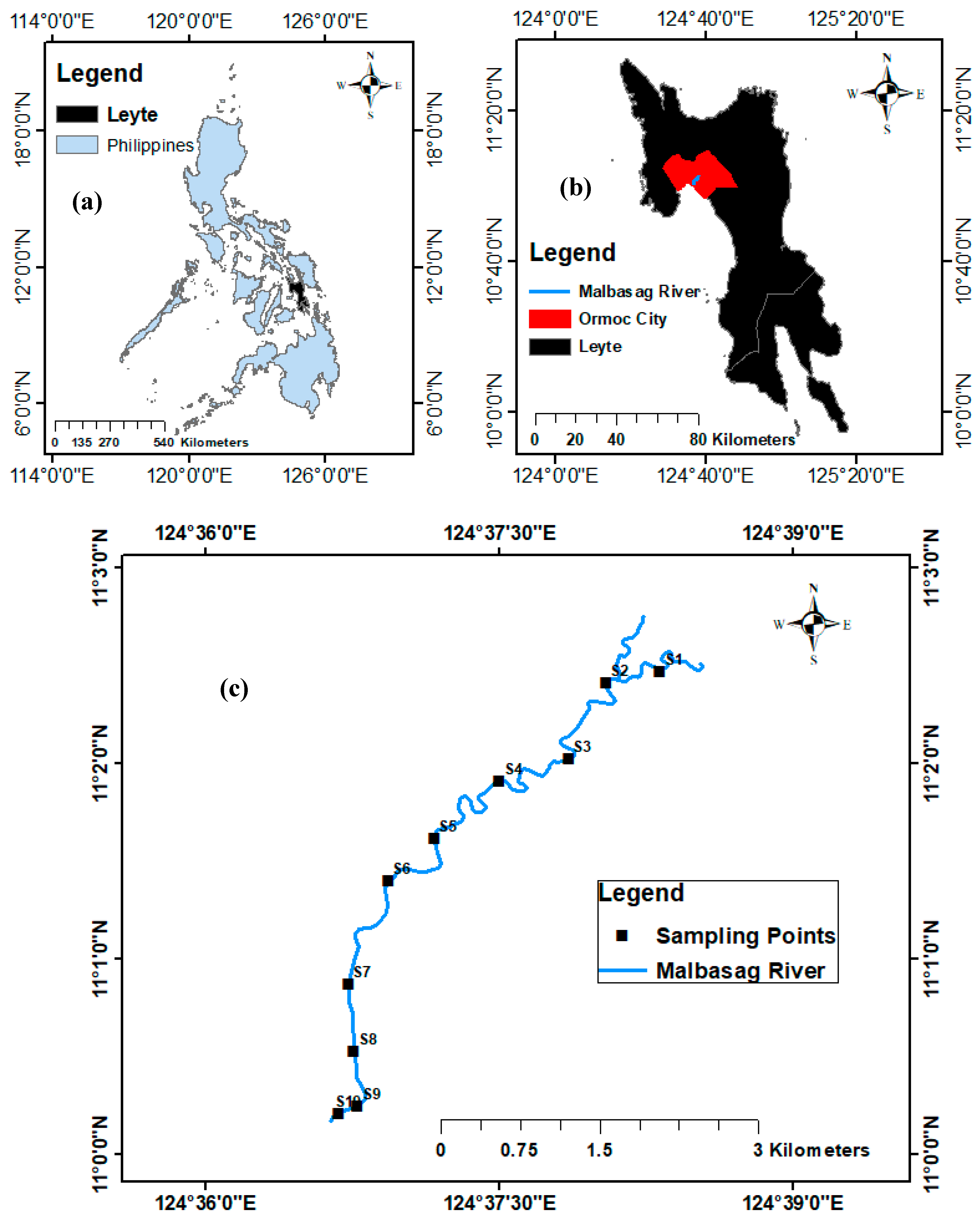
Figure 3.
Contamination factors (CF) of heavy metals of the surface sediment samples in the study area.
Figure 3.
Contamination factors (CF) of heavy metals of the surface sediment samples in the study area.
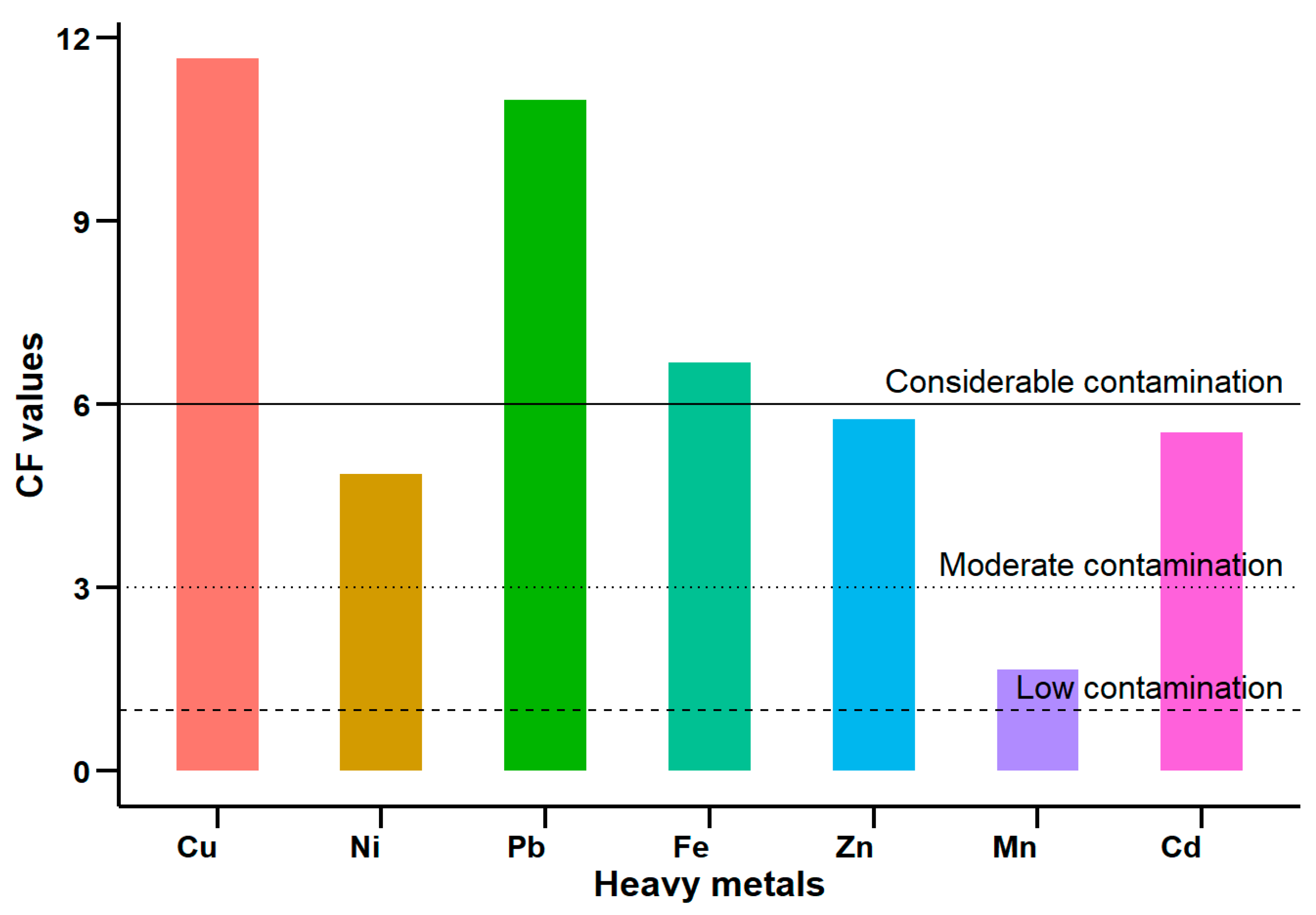
Figure 4.
Heavy metals pollution load index (PLI) value of the surface sediment of all Sites in the study area.
Figure 4.
Heavy metals pollution load index (PLI) value of the surface sediment of all Sites in the study area.
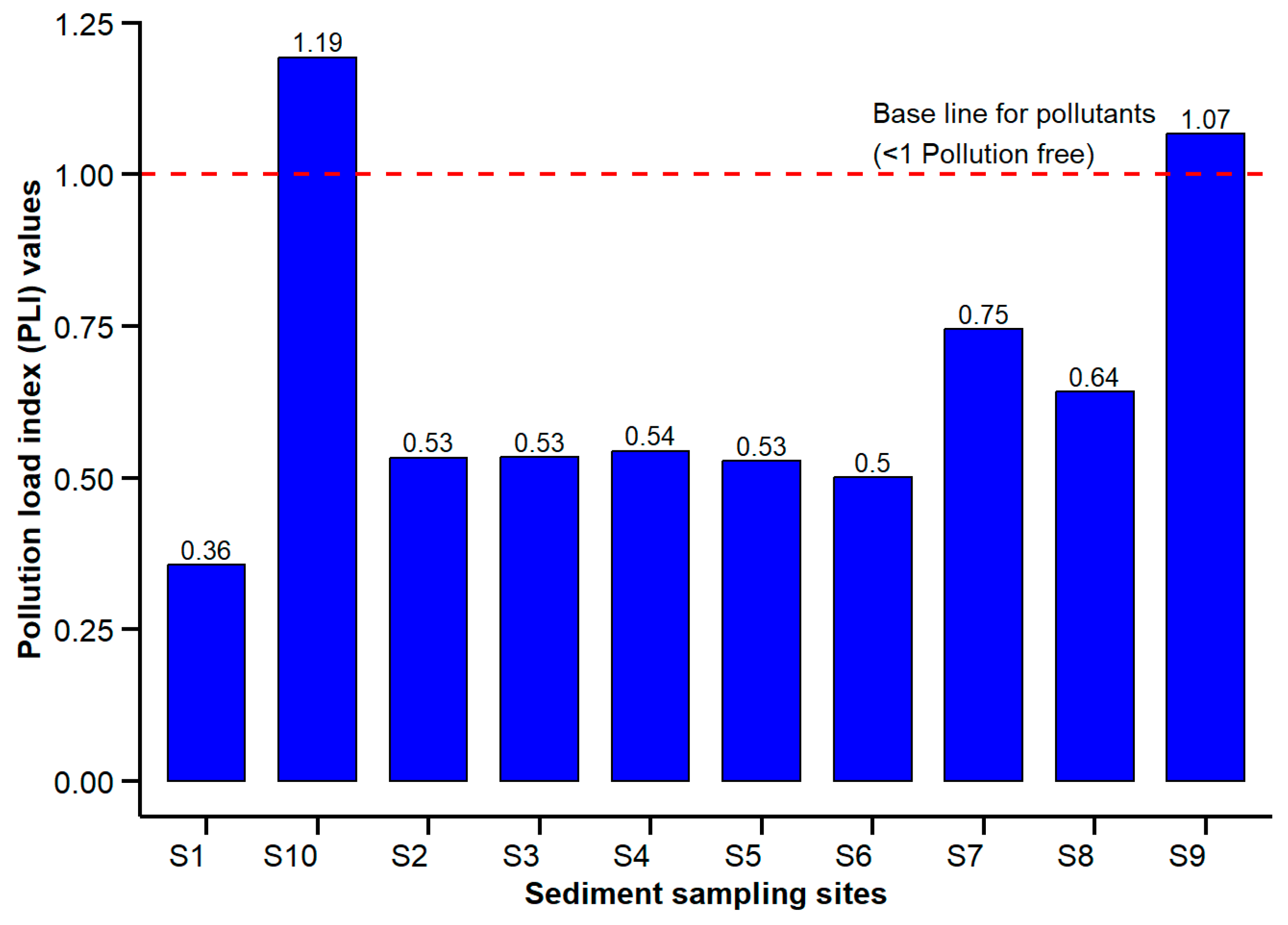
Figure 5.
The box-whisker plot of the geo-accumulation index (Igeo) value of the surface sediment samples in Malbasag River, Leyte, Philippines.
Figure 5.
The box-whisker plot of the geo-accumulation index (Igeo) value of the surface sediment samples in Malbasag River, Leyte, Philippines.
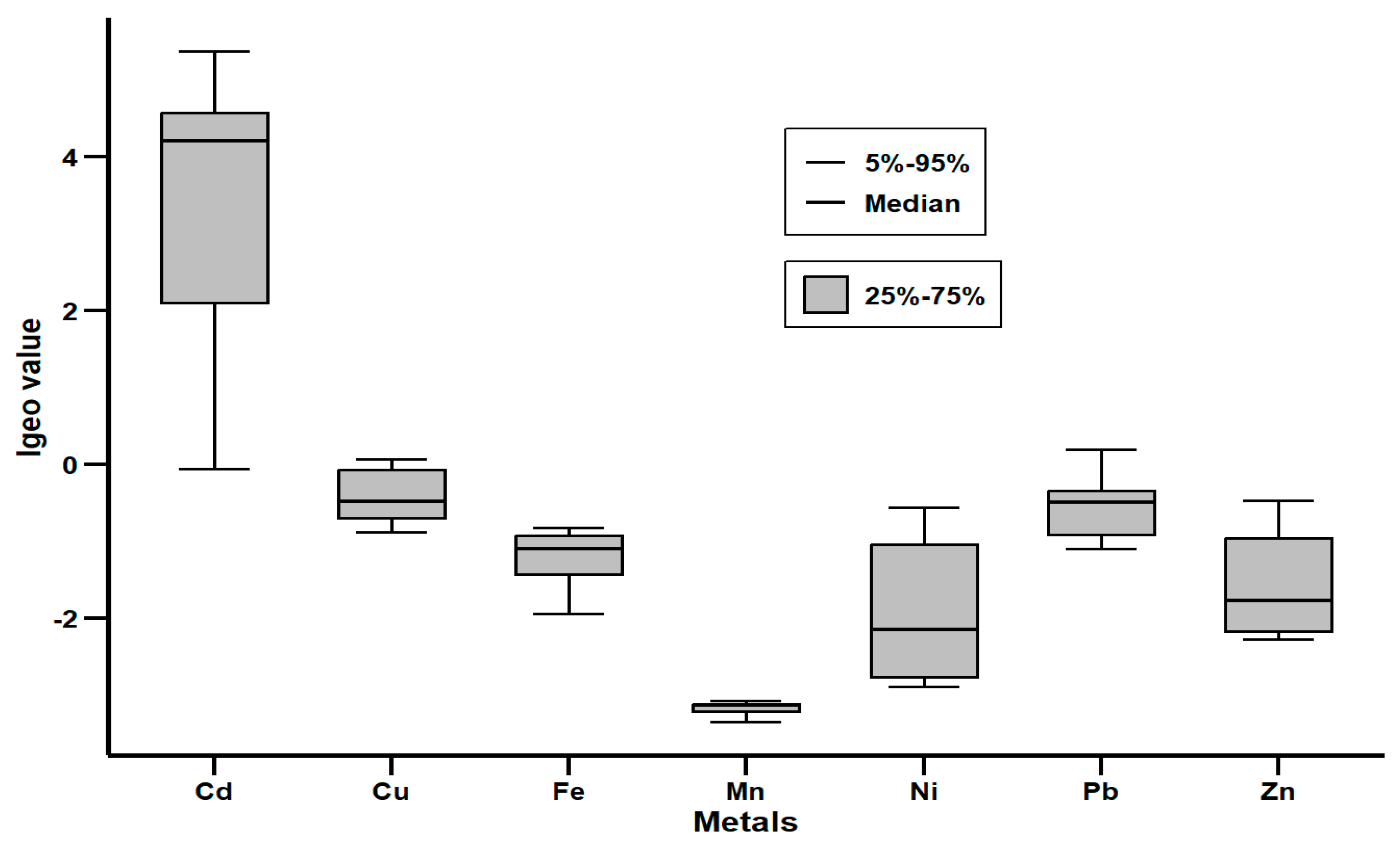
Figure 6.
Enrichment factor (EF) values for heavy metals in sediments of sampling Sites. The parallel dot lines denote EF value of 1.5.
Figure 6.
Enrichment factor (EF) values for heavy metals in sediments of sampling Sites. The parallel dot lines denote EF value of 1.5.
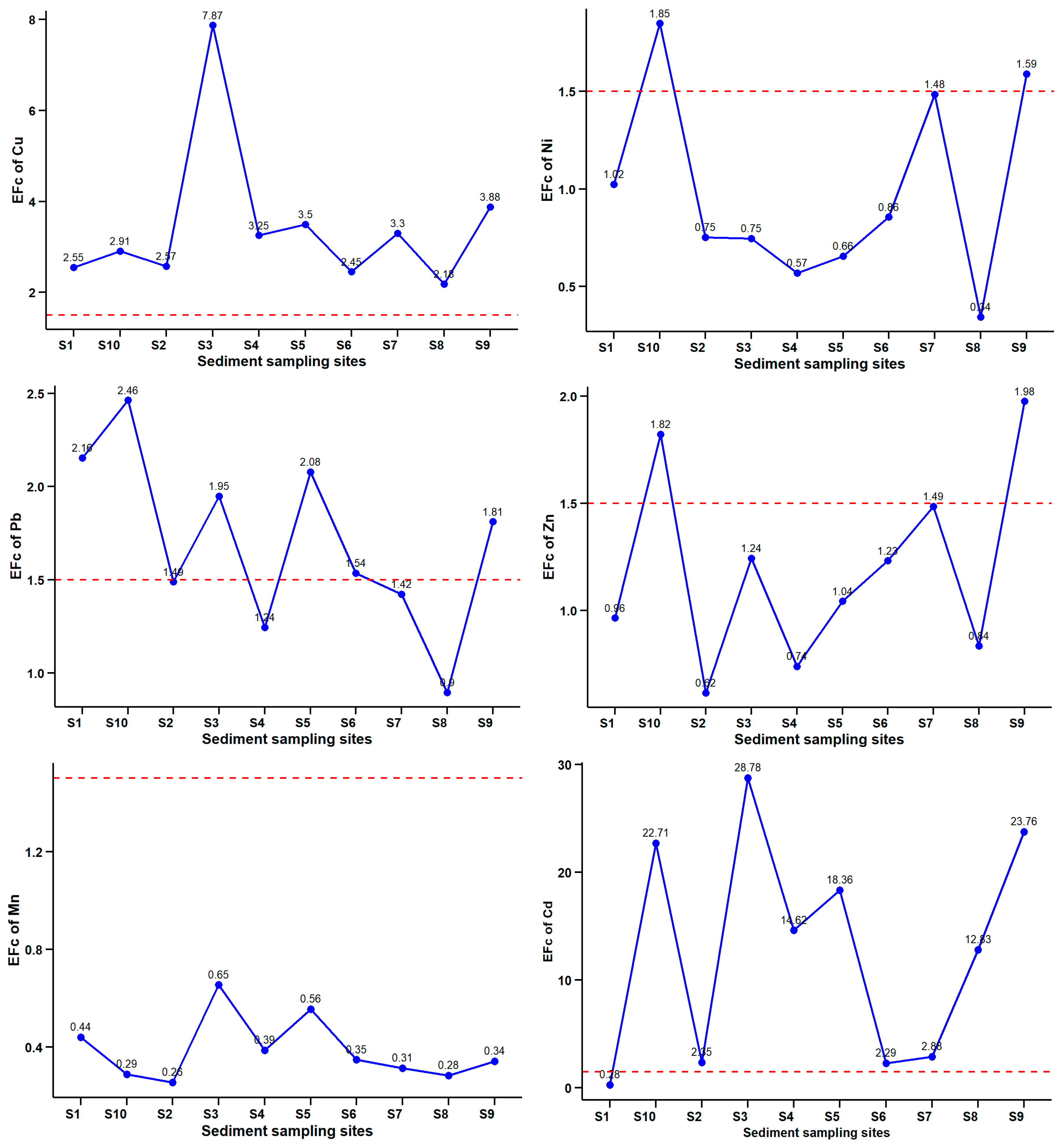
Figure 7.
(a) The toxic unit (TU) of each heavy metal and the sum of toxic units (ƩTUs) of the surface sediment samples. (b) The toxic risk index of surface sediment samples in the study area and the contribution ratio of each heavy metal.
Figure 7.
(a) The toxic unit (TU) of each heavy metal and the sum of toxic units (ƩTUs) of the surface sediment samples. (b) The toxic risk index of surface sediment samples in the study area and the contribution ratio of each heavy metal.
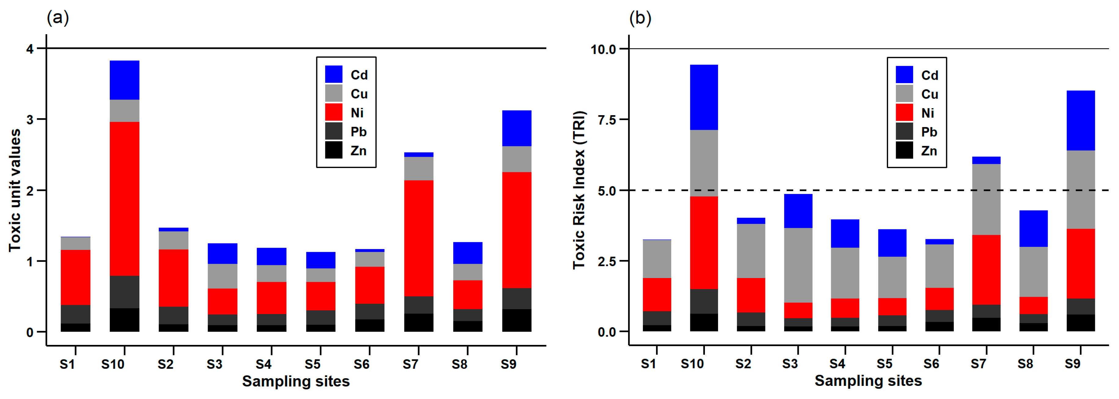
Figure 8.
Pearsons’s correlation coefficients of physicochemical properties and heavy metals in Malbasag River, Leyte, Philippines, P= value (0 '***' 0.001 '**' 0.01 '*' 0.05 '.' 0.1 ' ' 1).
Figure 8.
Pearsons’s correlation coefficients of physicochemical properties and heavy metals in Malbasag River, Leyte, Philippines, P= value (0 '***' 0.001 '**' 0.01 '*' 0.05 '.' 0.1 ' ' 1).
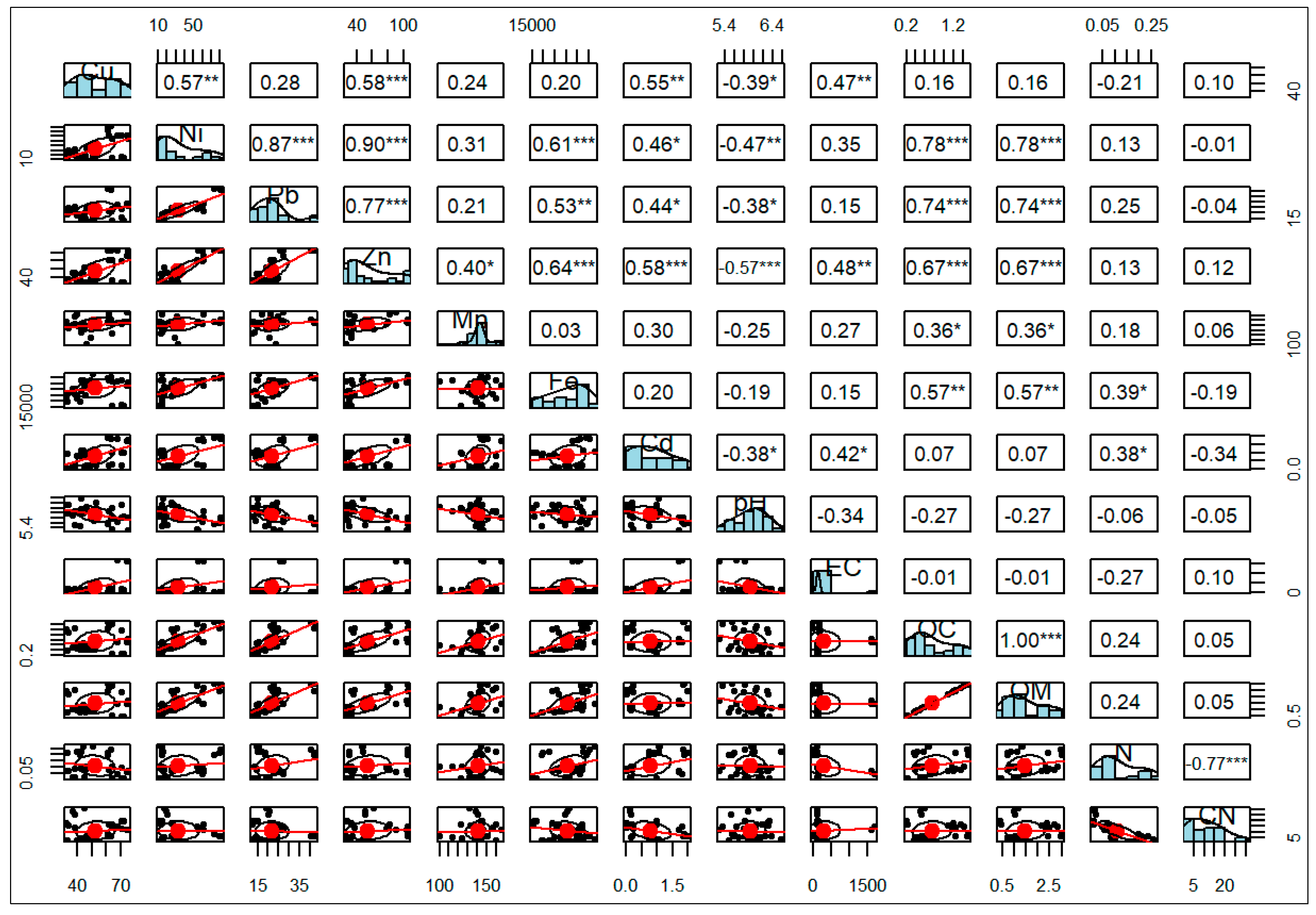
Figure 9.
Hierarchical cluster analysis for the heavy metals and sampling Sites in the study area.
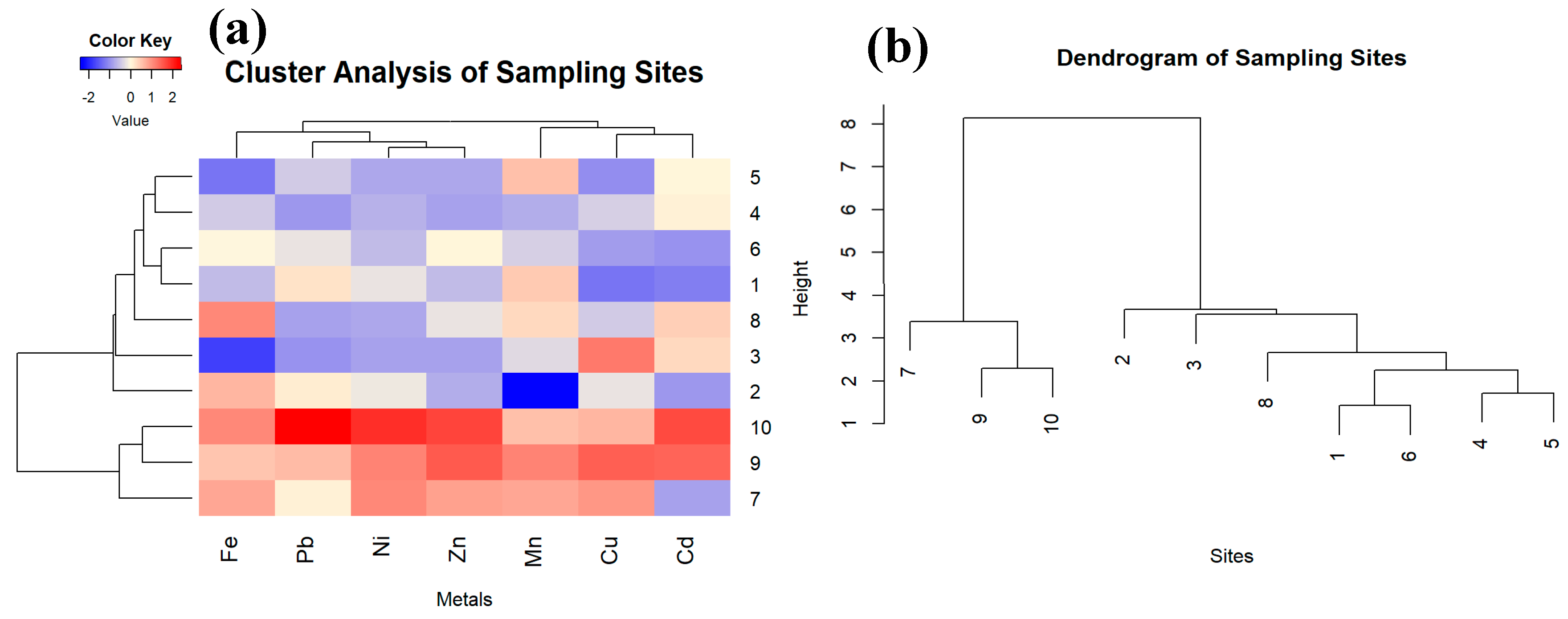
Figure 10.
Principal component analysis (PCA) in the sediment samples: Scree plot for identifying the proportion of variance and variable contributing showing the loading of individual parameters.
Figure 10.
Principal component analysis (PCA) in the sediment samples: Scree plot for identifying the proportion of variance and variable contributing showing the loading of individual parameters.
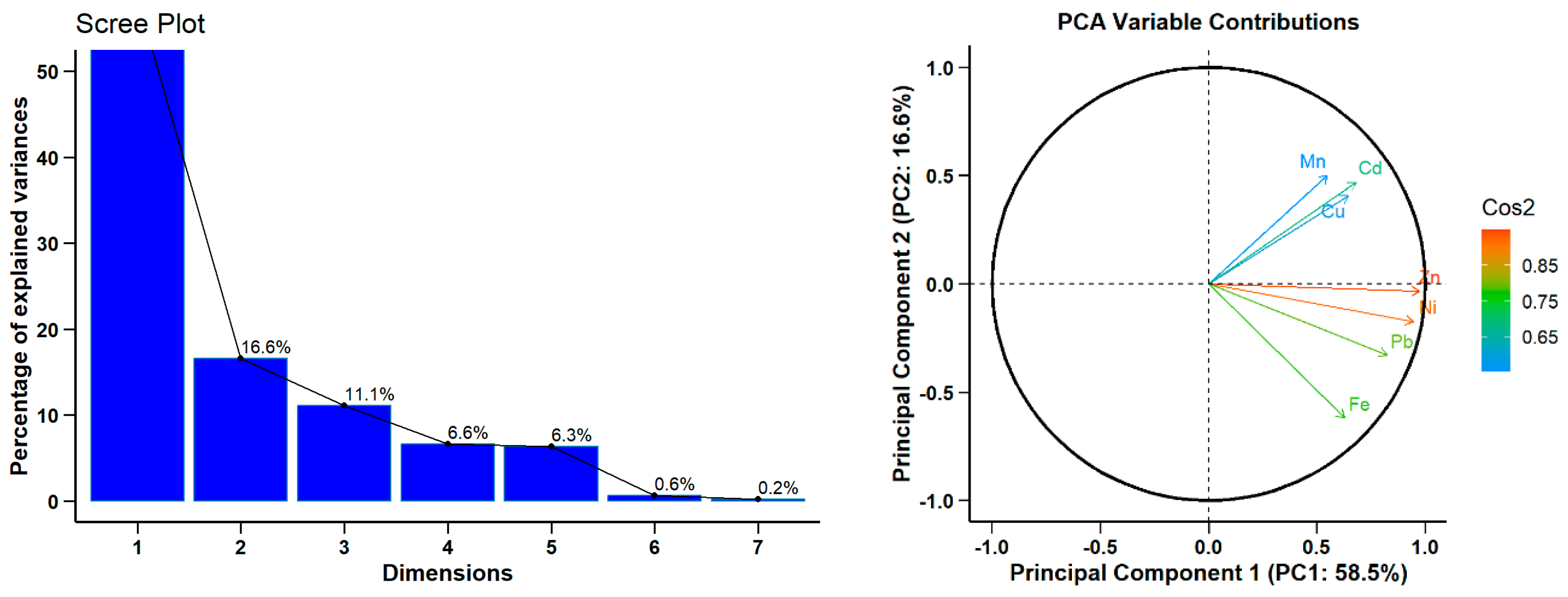
Figure 11.
Spatial distribution of heavy metals concentration (mg/kg) in Malbasag River, Leyte, Philippines. (a) Cu, (b) Ni, (c) Pd, (d) Zn, (e) Mn, and (f) Cd.
Figure 11.
Spatial distribution of heavy metals concentration (mg/kg) in Malbasag River, Leyte, Philippines. (a) Cu, (b) Ni, (c) Pd, (d) Zn, (e) Mn, and (f) Cd.
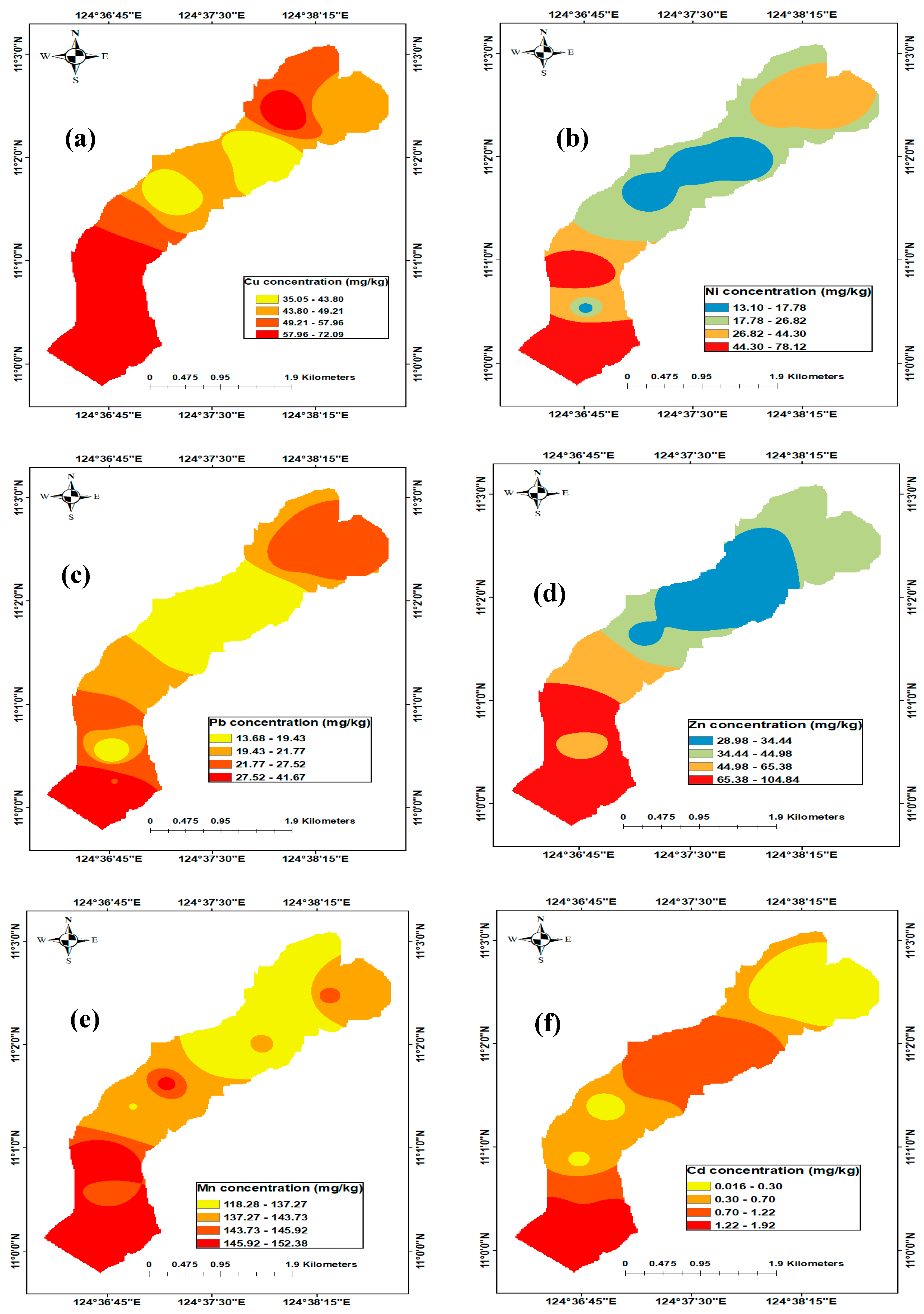
Table 1.
Sampling locations and Site description in the study area.
| Sample Id | Coordinates | Elevation (m, asl) | Site Description |
|---|---|---|---|
| S1 | 11.050334N 124.64137E |
261.9 | Site 1 is located beside agricultural fields. Agricultural runoff from pineapple fields may the source of pollution in this Site. It is located 4.66km away from Lake Danao which is the source of water for the rivers in Ormoc. |
| S2 | 11.040304N 124.63440E |
158.7 | Site 2 is located near a bridge which is under construction. Construction materials are source of pollution in this area. 1.76km away from Geraldez Livestock Trading. |
| S3 | 11.029750N 124.62264E |
75.8 | Site 3 is located beside agricultural fields. Agricultural runoff from sugar cane and pineapple fields could be the source of pollution in this Site |
| S4 | 11.028972N 124.62195E |
69.9 | Located 714m away from Sal’s Pineapple Farm. Also located beside ORWASA, water treatment facility which is the source of Ormoc’s water supply. |
| S5 | 11.026975N 124.61953E |
54.5 | This Site is a dam, located beside agricultural fields and residential area. |
| S6 | 11.025669N 124.61975E |
47.3 | Located beside agricultural field for rice. It is 104m away from Pura Agriventures and Development Corporation which has poultry and feeds making industry at Brgy. District 29, Nadongholan, Ormoc City. |
| S7 | 11.017924N 124.61288E |
24.4 | Site 7 is located just near a footbridge connecting Brgy. North and Brgy. Alta Vista. Wastewater drains from these barangays go into the river just before this site. Additional pollution sources at this Site include agricultural runoff from rice fields located 220m distant. |
| S8 | 11.008778N 123.61270E |
5.4 | Site 8 is located 150m away from Ormoc Central School. It is also between two barangays namely Brgy. East and Brgy. Alta Vista which are residential and personal care industrial areas which discharge domestic and industrial wastes into the river. |
| S9 | 11.004202N 124.61301E |
4.3 | Site 9 is located under Tulay de Perdon Bridge and 160m away from Ormoc Doctors Hospital and 210m from OSPA-FMC which are two big hospitals in Ormoc City. Residential areas are also existing around this Site namely Brgy. 28 and Brgy. Alta Vista. Several wastewaters drain that gather a combination of industrial and household effluent discharge into the river in front of this location. |
| S10 | 11.003522N 124.61139E |
4.8 | Site 10 is located 100m away from Ormoc City Port and City bus terminal, however during high tides, the port area’s sediments and water go into the river. It is in the Poblacion or center of Ormoc City. Residential and commercial wastes may be the pollution sources at this Site. At the right side of the river are the houses of Brgy. Can-Adieng and on the left side are landmarks such as Ormoc City Superdome, Ormoc City Museum, Baywalk Plaza, and Gaisano Ormoc Central Mall. Plastics, diapers, Styrofoam’s, and dead animals were seen in this Site. |
Table 2.
Physicochemical properties in surface sediment of the Malbasag River associated the Ormoc City port, Philippines.
Table 2.
Physicochemical properties in surface sediment of the Malbasag River associated the Ormoc City port, Philippines.
| pH | EC (µS/cm) | %OC | OM (%) | %N | C/N Ratio | |
|---|---|---|---|---|---|---|
| Mean (n=30) | 5.937 | 278.586 | 0.736 | 1.472 | 0.112 | 10.972 |
| Std | 0.323 | 467.334 | 0.408 | 0.817 | 0.081 | 8.148 |
| RSD (%) | 5.444 | 167.752 | 55.479 | 55.479 | 72.383 | 74.257 |
| Median | 5.985 | 126.650 | 0.582 | 1.163 | 0.092 | 9.565 |
| Min. | 5.290 | 4.340 | 0.210 | 0.420 | 0.011 | 1.781 |
| Max. | 6.590 | 1700.0 | 1.501 | 3.002 | 0.267 | 31.053 |
Min. = Minimum; Max. = Maximum; Std = Standard Deviation; RSD = Relative Standard Deviation.
Table 4.
Eir and RI values of heavy metals of surface sediments in Malbasag River, Philippines.
| Sites | Potential ecological risk factors (Eri) | RI | Risk level | |||||
|---|---|---|---|---|---|---|---|---|
| Cu | Ni | Pb | Zn | Mn | Cd | |||
| Site-1 | 3.894 | 2.483 | 5.930 | 0.380 | 0.171 | 1.562 | 14.420 | Low |
| Site- 2 | 5.520 | 2.563 | 5.746 | 0.341 | 0.139 | 18.170 | 32.479 | Low |
| Site- 3 | 7.675 | 1.156 | 3.420 | 0.312 | 0.162 | 101.035 | 113.759 | Moderate |
| Site- 4 | 5.200 | 1.447 | 3.582 | 0.305 | 0.157 | 84.175 | 94.866 | Moderate |
| Site-5 | 4.274 | 1.272 | 4.574 | 0.329 | 0.173 | 80.815 | 91.436 | Moderate |
| Site- 6 | 4.472 | 1.661 | 5.046 | 0.580 | 0.161 | 15.054 | 26.975 | Low |
| Site- 7 | 7.259 | 5.188 | 5.632 | 0.843 | 0.175 | 22.798 | 41.895 | Low |
| Site- 8 | 5.136 | 1.285 | 3.792 | 0.506 | 0.169 | 108.659 | 119.547 | Moderate |
| Site- 9 | 8.014 | 5.214 | 6.738 | 1.052 | 0.179 | 176.739 | 197.936 | Considerable |
| Site- 10 | 6.833 | 6.899 | 10.430 | 1.104 | 0.173 | 192.289 | 217.728 | Considerable |
Table 5.
Grading of ecological risk in the study area of surface sediment samples.
| Metals | 0.5> mHQ (Nil to very low severity of contamination) | 1> mHQ ≥ 0.5 (Very low severity of contamination) | 1.5> mHQ ≥1 (Low severity of contamination) | 2> mHQ≥1.5 (Moderate severity of contamination) | 2.5> mHQ ≥ 2 (Considerable severity of contamination) | 3 > mHQ ≥ 2.5 (Very high severity of contamination) | 3.5 > mHQ ≥3 (High severity of contamination) | mHQ ≤ 3.5 (Extreme severity of contamination) |
|---|---|---|---|---|---|---|---|---|
| Cu | (0), 0.0% | (0), 0.0 % | (17), 56.6% | (13), 43.3% | (0), 0.0% | (0), 0.0% | (0), 0.0% | (0), 0.0% |
| Ni | (0), 0.0% | (0), 0.0% | (15), 50% | (6), 20% | (6), 20% | (3), 10% | (0), 0.0% | (0), 0.0% |
| Pb | (0), 0.0% | (23), 76.6% | (0), 0.0% | (0), 0.0% | (0), 0.0% | (0), 0.0% | (0), 0.0% | (0), 0.0% |
| Zn | (0), 3.33% | (24), 80% | (6), 20% | (0), 0.0% | (0), 0.0% | (0), 0.0% | (0), 0.0% | (0), 0.0% |
| Cd | (3), 10% | (9), 30% | (12),40% | (6), 20% | (0), 0.0% | (0), 0.0% | (0), 0.0% | (0), 0.0% |
Table 6.
Linear regression results of the concentration of heavy metals and potential ecological risk index (RI) in surface sediment samples in the study area.
Table 6.
Linear regression results of the concentration of heavy metals and potential ecological risk index (RI) in surface sediment samples in the study area.
| Dependent Variable | Predictor | Coefficient (B) | Standard Error | t-value | p-value | VIF | R2 | Adjusted R2 | AIC | BIC | F-value |
|---|---|---|---|---|---|---|---|---|---|---|---|
| RI (Model 1) |
Cu |
0.187 |
0.023 |
6.527 |
<0.001** |
1.48 |
1.00 |
1.00 |
27.8 |
29.6 |
19570.22 p value 1.1e-10 |
| Pb | 0.475 | 0.034 | 8.041 | <0.001** | 1.25 | ||||||
| Mn | 0.052 | 0.028 | 0.590 | 0.127 | 1.25 | ||||||
| Cd | 99.30 | 0.512 | 230.2 | <0.001** | 1.88 | ||||||
| Log (RI) (Model 2) |
Cu |
0.006 |
0.008 |
-0.317 |
0.499 |
1.48 |
0.957 |
0.920 |
90.9 |
92.7 |
27.03 P value 0.0013 |
| Pb | -0.026 | 0.012 | -1.374 | 0.070 | 1.25 | ||||||
| Mn | -0.005 | 0.010 | -0.691 | 0.632 | 1.25 | ||||||
| Cd | 1.381 | 0.173 | 5.928 | <0.001** | 1.88 |
Disclaimer/Publisher’s Note: The statements, opinions and data contained in all publications are solely those of the individual author(s) and contributor(s) and not of MDPI and/or the editor(s). MDPI and/or the editor(s) disclaim responsibility for any injury to people or property resulting from any ideas, methods, instructions or products referred to in the content. |
© 2025 by the authors. Licensee MDPI, Basel, Switzerland. This article is an open access article distributed under the terms and conditions of the Creative Commons Attribution (CC BY) license (http://creativecommons.org/licenses/by/4.0/).
Copyright: This open access article is published under a Creative Commons CC BY 4.0 license, which permit the free download, distribution, and reuse, provided that the author and preprint are cited in any reuse.


