
Submitted:
25 January 2025
Posted:
27 January 2025
You are already at the latest version
Abstract
The CFD code C3d was used to investigate the operation of a routine utility flare at low and high gas firing rates in an oil field in Iraq. This code was developed for analysis of transient flares, enables the simulation of flare operation, and offers detailed estimates of the flame shape and the emissions produced. In this work, the numerical simulations included two flare gas rates, 9 t/h (2.5 kg/s) and 45 t/h (12.5 kg/s), under three crosswind conditions (4 m/s, 8 m/s and 14 m/ s) and using three stack heights (35 m, 45 m, and 55 m). The results of this work provided insights into flame shape and size, pollutant types and dispersion, and ground heat radiation levels from the flare. The safety analysis found that ground-level heat increases with higher flare gas rates and decreases with higher stack heights. The stack height of 55 m and the lower gas firing rate of 9 t/h were identified as the safest operating conditions as they provide lower ground level heat compared to the higher flare gas rate of 45 t/h. Likewise, environmental analysis showed that plume size increases with increasing flare gas rate, while pollutant dispersion intensifies with stronger crosswinds. When comparing the two gas firing rates, in the case of 9 t/h there was a smaller plume and less pollutant dispersion which illustrates the relatively lower impact on the environment.
Keywords:
gas flare
; emissions
; CFD
; environmental and safety aspects
; gas processing
1. Introduction
Gas flaring refers to the controlled combustion of natural gas that cannot be processed for sale or use due to technical or economic constraints. It is also the process of using specially designed combustion devices to safely and efficiently dispose of waste gases produced during regular plant operations. These waste gases come from various sources, such as associated gas, gas processing plants, well testing, and other facilities. The waste gas is typically collected in piping headers and directed to a flare system for safe disposal. A flare system usually consists of multiple flares to manage waste gases from different sources [1,2]. Flaring typically takes place at the top of a stack, where the gases are ignited, creating a visible flame. The height of the flame is directly related to the volume of gas being released, while its brightness and color are influenced by the specific composition of the gas. A complete flare system consists of the flare stack or boom, along with the pipes that collect and channel the gases to be flared [3], as illustrated in Figure 1.
The flare tip at the top of the stack is engineered to promote the entrainment of air into the flare, thereby improving combustion efficiency. Seals are installed along the stack to prevent the flame from flashing back into the system. At the base of the stack, a vessel collects and conserves any liquids that may result from the gas flow to the flare. Depending on the specific design and requirements of the process, one or more flares may be needed at a given location to manage the waste gases effectively. A flare is usually visible and produces not only light but also noise and heat. During the flaring process, the combustion of the gas primarily results in the formation of water vapor and CO2. For efficient combustion to occur, it is crucial to ensure proper mixing of the fuel gas with air (or steam), which facilitates complete combustion and minimizes the emission of unburned hydrocarbons and other pollutants [4,5,6,7,8].
Flaring processes can be classified into three main types: emergency flaring, process flaring, and production flaring [9]. Emergency flaring occurs in response to situations like fires, valve failures, or compressor breakdowns, where a large volume of gas is burned at high velocity over a short duration. Process flaring generally involves a lower rate of flaring, such as during the removal of waste gases from the production stream in petrochemical processes. The volume of gas flared in process flaring can range from a few cubic meters per hour during normal operations to thousands of cubic meters per hour during plant failures [10]. Production flaring, on the other hand, occurs within the exploration and production sector of the oil and gas industry. It involves burning large volumes of gas during gas-oil potential tests, which are performed to assess the production capacity of a well [3].
Gas flaring serves as both a method of waste disposal and a safety mechanism to relieve pressure by burning excess gas from wells, hydrocarbon processing facilities, or refineries [11]. On a global scale, gas flaring represents a significant environmental and energy challenge, with millions of tonnes of CO₂ and other greenhouse gases (GHG) released into the atmosphere each year, contributing to global warming. In 2023, approximately 148 billion cubic meters of gas were burned worldwide through gas flaring in oilfields, resulting in the emission of around 400 million tonnes of CO₂ into the atmosphere [12,13].
Flaring is generally regarded as the largest source of loss in several industrial sectors, including oil and gas production, chemical plants, refineries, coal industries, and landfills. This practice results in the waste of various gases, including process gases, fuel gas, steam, nitrogen, and natural gas. Flaring systems are widely used across different locations, such as onshore and offshore production fields, transport ships, port facilities, storage tank farms, and distribution pipelines. Furthermore, gas flaring is considered a cleaner energy source compared to many commercial fossil fuels, as the composition of flared gas closely resembles that of natural gas [14].
Recently, the significance of flare gas has grown, with increasing attention on the quantities of gas being wasted. This concern has risen due to the continuous increase in gas prices since 2005, alongside growing worries about the limited availability of oil and gas resources. Studies have shown that the amount of gas flared, if utilized as an energy source, could potentially meet 50% of Africa's electricity needs [15]. In fact, saving energy and reducing emissions have become global priorities. Additionally, minimizing flaring and maximizing the use of fuel gas contribute significantly to energy efficiency and climate change mitigation [16].
Gas flaring represents one of the most significant energy and environmental challenges facing the world today. Its environmental impacts are far-reaching, particularly for local communities, where it often leads to serious health issues. Gas flaring is typically visible and produces both noise and heat [11]. The release of greenhouse gases (GHGs) like CO2 and CH4 directly into the atmosphere traps heat, contributing significantly to climate change. These gases have a clear and substantial impact on the environment, making them major contributors to global GHG emissions [17]. Gas flaring has been a driving factor in rising global temperatures and has rendered large areas uninhabitable due to its environmental consequences. CO2 emissions from flaring have a high global warming potential, playing a major role in climate change. Around 75% of CO2 emissions stem from the combustion of fossil fuels [18]. CH4, a gas commonly found in flares with lower combustion efficiency, is even more harmful than CO2, with a global warming potential roughly 25 times greater than CO2 on a mass basis. This has raised concerns regarding the release of CH4 and other volatile organic compounds from various industrial operations [19,20].
Other pollutants, such as sulfur oxides (SOx), nitrogen oxides (NOx), and volatile organic compounds (VOCs), are also released during the flaring process [11,18,21,22,23]. A study by Ezersky and Lips in 2003 [22] on emissions from oil refinery flare systems in the Bay Area Management District (California) found that emissions ranged from 2.5 to 55 tons per day of total organic compounds and from 6 to 55 tons per day of SOx. As a result, flare emissions can contribute significantly to overall SO2 and VOC emissions. Once emitted, gaseous pollutants like SO2 have no boundaries, becoming uncontrollable and contributing to acid deposition. Numerous toxicological and epidemiological studies have revealed the severe effects of these gases [24]. SOx and NOx are key contributors to acid rain and fog, which damage the natural environment and harm human health. Additionally, ozone, produced by the photochemical reaction of VOCs and NOx, exacerbates the damage by accelerating the oxidation of SO2 and NOx into toxic sulfuric and nitric acids, respectively. Therefore, reducing VOC and NOx emissions is essential for lowering ozone concentrations [25].
On the other hand, a smoking flare can significantly contribute to overall particulate emissions. Most flared gas is untreated or unprocessed, leading to challenging service conditions. This can result in issues such as condensation, fouling (e.g., from the buildup of paraffin wax and asphaltine deposits), corrosion (e.g., due to the presence of H2S, moisture, or air), and possibly abrasion (e.g., from debris, dust, and corrosion products in the piping and high flow velocities) [26].
The quantity of emissions generated from flaring is largely determined by the combustion efficiency [4]. Several factors influence this efficiency, such as the heating value, velocity of gases entering the flare, meteorological conditions, and their impact on flame size. When flares are properly operated, they can achieve combustion efficiency levels of at least 98%, meaning that hydrocarbon and CO emissions represent less than 2% of the species in the gas stream [10]. This highlights the high efficiency of well-designed and well-operated industrial flares. However, flare efficiencies can vary significantly, ranging from 62% to 99% [27,28]. Gas flaring can have a considerable environmental impact, particularly due to the potential presence of harmful compounds, with the extent of the impact depending on the composition of the flared gas [4].
The aim of this paper is to evaluate a utility flare (55 m in height and 0.61 m in diameter) operation in one of the oilfield sites in Iraq during two gas firing rates low with 9 t/hr and high 45 t/hr under different operational conditions using CFD code C3d version (5-20-24). This includes the environmental and safety aspects of the flare operation under different operational conditions by studying the effect of stack height and crosswind on the amount of thermal radiation and pollution released from the burning flare gas during both firing rates. Moreover, this work evaluates the amount of pollutants in the plume generated during both gas firing rates.
2. Methodology
This paper uses CFD code C3D based on LES approach version (5-20-24) to analyze the operation of a routine utility flare during low and high firing rates in the summer in Iraq. The analysis focuses on both safety and environmental reviews of the flare operation under different gas firing conditions: a low rate of 9 t/hr and a high rate of 45 t/hr. The study also examines the impact of three different crosswind speeds (4 m/s, 8 m/s, and 14 m/s) and three different stack heights (35 m, 45 m, and 55 m) to understand how these factors affect radiation rates to the ground and pollution dispersion.
The chosen flow rates reflect practical and safety considerations for routine operations. The low gas firing rate represents the typical operational rate during routine flare activities. The high gas firing rate, while below the maximum allowable rate of 250 t/hr, was selected because it is more likely to occur under routine conditions compared to the maximum rate, which is typically associated with emergency flare operations. The flare height and diameter used in this study were 55 m and 0.61 m (24″), respectively. Table 1 shows flare gas composition used in this study.
Additionally, ParaView software 5.12.1 was used to visually represent the flare operation at both gas firing rates. The software enables visualization of ground radiation and allows for the extraction of combustion products, which are essential for evaluating the pollution rate from burning flare gas. This integrated approach helps to assess the environmental impact of flare operation under various conditions and provides a clear representation of the flare’s behavior during routine and maximum operation scenarios.
2.1. CFD Code C3d
C3d is a computational fluid dynamics (CFD) and heat transfer software developed by the USDOE Sandia National Laboratory, designed to tackle a wide range of fluid mechanics and heat transfer problems, including flare and fire analysis. It uses the Large Eddy Simulation (LES) methodology to perform transient analyses of flare operations. In flare studies, C3d is commonly applied to estimate flame shapes and the associated emissions. The software includes several optional sub-models that simulate various processes, such as deposition, radiation heat transfer, aerosol transport, chemical reactions, combustion, and material decomposition.
For fire and flare scenarios, C3d models important phenomena such as fuel vapor transport, liquid fuel evaporation, combustion products, heat release, and chemical reactions. It also accounts for soot and intermediate species formation and destruction, diffusion radiation within the fire, and radiation view factors from the fire's edge to nearby objects. The software selects soot radiation and reaction rates based on comparisons with experimental data from flare and fire studies. To model fluid flow around solid objects, C3d employs a body-fitted geometry method, combined with a structural orthogonal Cartesian grid. This approach allows for both fine and coarse discretization while accurately representing the curvature of objects within the flow domain.
The C3d code has been widely used in various studies [29,30], including those evaluating flare performance and fire safety. Originally developed as a CFD tool called ISIS-3D, it was validated for simulating pool fires and assessing the thermal performance of nuclear transport packages [31,32,33]. The C3d code has been applied in multiple studies to analyze different types of flares, such as utility flares, air-assisted flares, and large multipoint ground flares [34,35,36,37]. Its combustion model has been enhanced and validated for a variety of flare gases like propane, methane, ethylene, ethane, propylene, and xylene. The code helps estimate flame size, shape, and the impact of smoking tendencies, as well as heat flux to the ground [38].
C3d has also been employed in studies involving multipoint ground flares to assess the effect of surrounding wind fences on flame height and shape under high firing conditions [36]. It has proven useful in determining the optimal spacing between flare tips to ensure sufficient airflow during operation, thus preventing smoke under maximum firing conditions. Moreover, the code has been used to investigate the impact of discrete and continuous ignition systems on flare operation [35].
2.2. Physical Model
In all simulations, the LES turbulence model was employed to simulate fluid flow, while radiation effects were incorporated into the energy equation. To monitor the distribution and concentration of the fuel, soot, intermediate species, and combustion products (such as H2O and CO2), individual species equations were solved. The combustion model provided the sink and source terms for these species equations, based on local gas temperature, species concentrations, and turbulent diffusivity.
The code predicted flame emissivity using various models that considered factors such as soot volume fraction, molecular gas composition, flame size, shape, and the temperature profile of the combustion effluent. These factors were derived from the solutions to the momentum, mass, species, and energy equations. Additionally, a radiation transport model was used to predict the radiation flux from the flame to the ground and to provide the sink and source terms for the energy equation, allowing for the prediction of the flame's temperature distribution.
2.3. Chemical and Soot Model
A combination of Arrhenius and Eddy breakup reaction time scales have been used to define the rate of combustion equations.
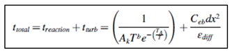 (T) = a local gas temperature, (Ak) = a pre-exponential coefficient, (b) = a global exponent, (Ceb) = the eddy breakup scaling factor, (TA) = activation temperature, (dx) = the characteristic cell size, (tturb) = the turbulence time scale, and (εdiff) = the eddy diffusivity from LES module [34].
Combustion chemistry consists of several critical reactions. Initially, primary fuel breakdown reactions generate intermediate combustion products such as C₂H₂, H₂, CH₄, soot, and CO. These intermediate products undergo secondary reactions that further combust, contributing to soot formation. Additionally, reforming reactions that involve hydroxyl (OH) radicals play a significant role in the process. In this scenario, oxidizing species are simplified to water vapor. To promote soot formation, equilibrium reactions involving acetylene, methane, hydrogen, sulfur, and hydrogen sulfide are also included in the model [34].
The primary fuel breakdown, secondary and reforming reactions of the flared gas mixture are shown below:
| The primary fuel breakdown reactions | |
| CH4 + O2 → 0.33C2H2 + 0.33CO + 1.67H2O | CH4 Breakdown |
| C2H6 + 1.5O2 → C2H2 + 2H2O + CO | C2H6 Breakdown |
| C3H8 + 2O2 → C2H2 + 3H2O + CO | C3H8 Breakdown |
| C4H10 + 3O2 → C2H2 + 4H2O + 2CO | C4H10 Breakdown |
| C5H12 + 2.5O2 → 2C2H2 + 4H2O + CO | C5H12 Breakdown |
| H2S + O2 → SO2 +H2 | H2S Breakdown |
| N2 + O2 → 2NO | N2 Breakdown |
| The secondary reactions | |
| H2 + 0.5O2 → H2O | H2 Combustion |
| C2H2 + 0.8O2 → 1.6CO + H2 + 0.02C20 | Soot nucleation soot formation |
| C2H2 + 0.01C20 → H2 + 0.11C20 | Soot growth by acetylene addition |
| CO + 0.5O2 → CO2 | CO combustion |
| C20 + 10O2 → 20CO | Soot combustion |
| C2H2 + 3H2 → 2CH4 | Acetylene decomposition |
| CH4 + CH4 → C2H2 + 3H2 | Acetylene formation |
| 0.5S2 + H2 → H2S | Sulfur reduction to hydrogen sulfide |
| H2S → 1.5S2 + H2 | Hydrogen sulfide decomposition |
| H2S + 0.5SO2 → 0.75S2 + H2O | Elemental sulfur formation |
| The reforming reactions | |
| C20 + 20H2O → 20CO + 20H2 | Soot steam reforming |
| 0.75S2 + H2O → H2S + 0.5SO2 | Sulfur steam reforming |
A global Arrhenius rate mode is used for these reactions. The consumption of fuel, soot, and intermediate species are evaluated by:
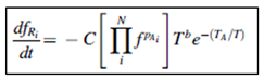 (N) = number of reactants, (TA) = effective activation temperature, (fRi) = moles of each reactant, (i) and (c) = pre-exponential coefficient, and (b) = temperature exponent.
2.4. Computational Domain and Flare Model
Three different computational domain sizes were used to simulate various cases with different stack heights at both low and high gas firing rates. The first domain size had dimensions of 65 m in height, 50 m in length, and 50 m in width, and was used for a stack with a height of 35 m and a diameter of 0.61 m. The second domain size was 75 m in height, 50 m in length, and 50 m in width, corresponding to a stack height of 45 m and the same stack diameter of 0.61 m. The third domain size was 85 m in height, 50 m in length, and 50 m in width, with a stack height of 55 m and a diameter of 0.61 m.
In all three cases, the computational domain's height (z-axis) extended from -0.1 m to 0 m, defining the ground level (dry sand) for the flare, and then from 0 m to the top of the domain. The domain's length (x-axis) ranged from -5 m to 45 m, and its width (y-axis) spanned from -25 m to 25 m. By positioning the x and y domains at -5 m and -25 m, the flare's center was strategically placed to ensure that the crosswind would blow from the x-axis. The flare model was constructed from carbon steel using a dedicated flare modeler.
This approach allowed for the simulation of various stack configurations and operational scenarios. Figure 2 shows three computational domain sizes with corresponding mesh configurations used for the different simulation cases in this study. These domain sizes were selected to represent various operational scenarios, allowing for a detailed analysis of flare. Moreover, Figure 3 illustrates the three flare stack heights within the domain, along with the mesh for both the stack and the ground. This figure provides a clear representation of the stack configurations and their relationship to the computational domain, highlighting the precision of the mesh distribution around key components to ensure accurate simulation results. The total number of hexahedral cells for the simulations varied depending on the stack height. In the case of the 35 m tall stack, there were 1,335,288 cells (138 × 118 × 82). For the 45 m tall stack, the number of cells increased to 1,498,128 (138 × 118 × 92), and for the 55 m tall stack, there were 1,660,968 cells (138 × 118 × 102). In all cases, the mesh was refined near the flare tip to accurately capture the flame shape and the transient nature of the flow. This finer mesh ensured that the complex interactions in the flame region were simulated with a high level of detail, improving the accuracy of the results.
2.5. Mesh Independence Study
A mesh independence study was conducted by monitoring the change in carbon dioxide emissions during a 9 t/hr gas firing operation. Since three different stack heights (35 m, 45 m, and 55 m) with corresponding domain sizes were applied in this study, a separate mesh independence analysis was performed for each case. For each stack height, two different mesh configurations were tested: one with a lower cell number and another with a higher cell number.
Figure 4, Figure 5 and Figure 6 show the specified probe locations used to monitor the carbon dioxide emissions in the plume during the mesh independence study. The probe used in this study had a radius of 0.3 m and was employed to record 10 datasets for each monitoring location. The average of these datasets was then calculated and used in the analysis.
Figure 7, Figure 8 and Figure 9 show the results of the mesh independence study for the 35 m stack height, 45 m stack height, and 55 m stack height cases, respectively. According to these figures, there is a slight difference in the carbon dioxide mass fraction between the lower and higher cell numbers for each case. This indicates that the mesh refinement has a minimal effect on the results, demonstrating mesh independence. Therefore, the chosen mesh configurations 1,335,288 cells for the 35 m stack height, 1,498,128 cells for the 45 m stack height, and 1,660,968 cells for the 55 m stack height were deemed appropriate for the simulations, as they provide reliable and consistent results.
2.6. Boundary Conditions
The boundary conditions implemented in this work included three crosswind cases with speeds of 4 m/s, 8 m/s, and 14 m/s at a temperature of 300 K, flowing from the x-axis toward the flare. Hydrostatic pressure was defined throughout the computational domain to ensure accurate simulation of pressure variations. To model the specific components of the flare system, three one-dimensional subgrids were established: one for the ground, one for the flare wall, and one for the flare tip. In the ground subgrid, dry sand was selected as the material, representing the ground beneath the flare. In the flare wall subgrid, carbon steel was chosen as the material for the flare stack, reflecting the typical construction material for such systems.
For the flare tip subgrid, the mass flux and temperature of the gas were specified for both low and high gas firing rates. The mass flux values were 8.4 kg/m².s (equivalent to 9 t/hr or 2.5 kg/s) at the low gas firing rate, and 42 kg/m².s (equivalent to 45 t/hr or 12.5 kg/s) at the high gas firing rate, with the gas temperature maintained at 300 K. Finally, the flare exit was defined as a three-dimensional pressure outlet, ensuring proper representation of gas flow and pressure conditions at the flare tip.
2.7. Post Processing and Transient Calculation
Initially, the simulation ran for 100 timesteps to calibrate the gas mass flow rate injected through the flare in all cases, which was set to 2.5 kg/s and 12.5 kg/s. This initial phase allowed the system to adjust and ensure accurate gas flow representation. Following the calibration, the simulation parameters were adjusted, with the timestep set to 1,000,000 and the total simulation time extended to 10 seconds. This longer duration was necessary to allow the system to stabilize and accurately reflect the operational characteristics of the flare under the specified conditions.
To check the simulation stability and validate the gas firing rate, the net reaction energy source was used in all simulation cases. The net reaction energy source consists of reaction power (MW), which changes with time. This power can be calculated for each case by multiplying the gas flow rate (kg/s) by the LHV of the gas (MJ/kg). For instance, in the case of a 2.5 kg/s gas firing rate, the reaction power is approximately 113 MW, calculated as 2.5 kg/s times 45 MJ/kg. Similarly, for the 12.5 kg/s gas firing rate, the reaction power is approximately 563 MW, calculated as 12.5 kg/s times 45 MJ/kg. At the start of the simulation, the initial combustion of a significant amount of gas causes a small peak in the reaction power curve. However, after a few seconds, this value drops and stabilizes, indicating that the simulation has reached a steady state. Figure 10 shows net reaction energy source and time step size for 2.5 gas firing rate cases, while Figure 11 displays the net reaction energy source and simulation time step size for 12.5 kg/s gas firing cases.
3. Results
ParaView version 5.12.1 was used to extract the results for this study, which includes comparing the flare operation under low and high gas firing rates. This includes comparing flame size and shape, soot formation and combustion products. Moreover, the results include studying the effect of crosswind on pollution dispersion and wake stabilization. Finally, the results demonstrate the relation between stack height and ground heat during both firing rates.
3.1. Flame Shape and Size vs. Crosswind
The flame size and shape during low and high gas firing rates, using a flare stack with a height of 55 m and a diameter of 0.61 m, were visualized using the CFD code C3d and ParaView software. To study the changes in flame angle and pollution dispersion, three different crosswind speeds (4 m/s, 8 m/s, and 14 m/s) were applied. Figure 12 and Figure 13 illustrate the effects of crosswind on flare operation under low and high gas firing rates, respectively.
The figures demonstrate that as the gas firing rate increases, the flame size and shape also expand, leading to higher heat radiation toward the ground and greater pollutant emissions. In both low and high gas firing rate scenarios, an increase in crosswind speed stabilizes the wake and elongates the flame. Additionally, ground heat radiation rises with the flare gas firing rate but decreases with higher crosswind speeds due to the cooling effect of the wind on the flame.
3.2. Flame Temperature and Combustion Products vs. Crosswind
The environmental consequences of flare operation have always been a topic of interest, and understanding the types of emissions produced by a flare is a critical aspect when analyzing its operation. This paper show and compare the combustion products of the flare under low and gas firing rates and using a flare stack height and diameter of 55 m and 0.61 m respectively. To demonstrate the effect of crosswind on pollution dispersion, three crosswind speeds (4 m/s, 8 m/s, and 14 m/s) were applied.
3.2.1. Flame Temperature
Figure 14 and Figure 15 illustrate the impact of crosswind on flame temperature during low and high gas firing rates.
From these figures, it is clear that as the gas rate increases, the flame temperature also increases due to the larger flame size. The figures show that the flame temperature at a normal firing rate ranged from 1600 to 1800 K, while at a high firing rate, it exceeded 2000 K. Furthermore, the figures clearly demonstrate wake stabilization, especially during high gas firing rates. This phenomenon has important implications for flare operation, not only in maintaining safe operation but also in reducing the lifetime of the flare tip. In other words, increased wake stabilization causes the flame to remain attached to the tip, and with the higher temperatures, the flare tip's lifetime becomes shorter and it becomes more susceptible to deformation.
3.2.2. Soot Formation
Soot formation is one of the main pollutants produced during flare operation, and studying this pollutant is essential for evaluating the environmental performance of the flare. Figure 16 and Figure 17 illustrate the soot formation rate from the flare during normal and high gas firing rates under different crosswind conditions.
According to these figures, soot formation during high gas firing rates is significantly higher than during normal gas firing rates. In the case of normal flare gas operation, soot formation ranged from 1 to 1.3 ppmv, while at higher flare gas operation, it exceeded 1.4 to 1.5 ppmv. The effect of wind is evident in both operational cases, with soot dispersion increasing as the crosswind speed rises.
3.2.3. Carbon Dioxide and Carbon Monoxide Emissions
The important combustion products that indicate the quality of combustion at the flare tip are carbon dioxide (CO₂) and carbon monoxide (CO). Figure 18 and Figure 19 show the emissions of carbon dioxide (CO₂) during normal and high gas firing rates of the flare, considering different crosswind speeds. Moreover, Figure 20 and Figure 21 demonstrate the emissions of carbon monoxide (CO) during normal and high gas firing rates under various crosswind speeds.
The CO₂ emissions in Figure 18 and Figure 19 show that crosswind significantly affects the dispersion of this pollutant. By comparing these two figures, it is clear that a high flare gas rate produces more CO₂ than a normal flare gas rate.
Generally, the CO emissions in Figure 20 and Figure 21 are much lower than the CO₂ emissions, indicating that the operation was acceptable to some extent, especially during normal gas firing rates. In fact, the low CO emissions at low gas firing rates, compared to high gas firing rates, explain the lower soot formation in the low gas firing rate case. In other words, at low gas firing rates, the flare gas combustion is more stable, allowing most of the flare gas to convert to CO₂ instead of CO, which results in less soot formation. In contrast, at high gas firing rates, more CO is produced, leading to increased soot formation.
3.2.4. Sulphur Dioxide and Nitric Oxide Emissions
Sulphur dioxide (SO₂) and nitric oxide (NO) are hazardous combustion products of flare operation. Since the flare gas contains hydrogen sulfide (H₂S) and nitrogen, the presence of these emissions after combustion is expected. show the Sulphur dioxide emissions during normal and high gas firing rates and under different crosswind speeds. Figure 22 and Figure 23 show the sulfur dioxide (SO₂) emissions during normal and high gas firing rates under different crosswind speeds. Similarly, Figure 24 and Figure 25 illustrate the nitric oxide (NO) emissions from flare operation during normal and high gas firing rates under various crosswind speeds.
Comparing sulfur dioxide (SO₂) emissions at a normal gas firing rate in Figure 22 with SO₂ emissions at a high gas firing rate in Figure 23, it is clear that the rate of emissions increases as the flare gas rate increases due to the larger amount of gas being burned. Furthermore, these figures clearly demonstrate that crosswind significantly affects the dispersion of this pollutant. An increase in crosswind enhances the dispersion of SO₂, allowing it to spread to greater distances.
Regarding nitric oxide (NO) emissions, similar to other combustion products, the emission rate is higher at a high gas firing rate than at a normal gas firing rate. Additionally, the dispersion of nitric oxide due to crosswind follows the same pattern as SO₂ and other emissions. Finally, the dispersion increases with rising crosswind speeds, ranging from 4 m/s to 14 m/s.
3.3. Heat Radiation vs. Stack Height
One of the critical safety factors in flare operation is the heat radiation to the ground. This study examines the effect of stack height on ground heat radiation using three stack heights: 55 m, 45 m, and 35 m. In all cases, the crosswind speed was kept constant at 9 m/s. Figure 26 and Figure 27 illustrate the ground heat radiation for different stack heights during low and high gas firing rates, respectively, under constant crosswind conditions.
The figures clearly show that a decrease in stack height leads to an increase in ground heat due to greater heat radiation from the flame to the ground. A shorter flare stack brings the flame closer to the ground, resulting in more heat being absorbed by the surface. Additionally, an increase in the amount of flare gas amplifies ground heat as it generates a larger flame. This is evident from the figures, where for the same scenario, the heat radiation from a high gas firing rate is significantly greater than that from low or normal firing rates.
For instance, in the case of low firing rates with a shorter 35 m flare stack, the ground heat reaches 1000 W/m² within a 20 m radius. In contrast, with the same stack height and a high gas firing rate, ground heat exceeds 2000 W/m² within a 25 m radius. This demonstrates that as the gas firing rate increases, the radius of ground heat expands, necessitating additional precautions to ensure safe operation at the site.
3.4. Sampling Locations
As explained earlier, the increase in the amount of gas being flared affects the rate of emissions. Four locations in the domain were defined for both gas firing rates, under a crosswind speed of 8 m/s, to extract combustion product data. The flare's hydraulic limits in this study were a height of 55 m and a diameter of 0.61 m. Figure 28 shows the probe locations used for monitoring combustion products during normal gas firing rates, while Figure 29 illustrates the probe locations used for monitoring combustion products during high gas firing rates. The probe size in both gas firing cases was 0.3 m in radius and recorded ten datasets at each location. The average of these ten datasets was taken and represented.
The following tables show the main combustion products and fuel compounds in the plume at both gas firing rates. Additionally, they provide the locations of the probes in the domain, as well as the size of the probes used to extract combustion products and fuel compounds from the plume. Table 2 and Table 3 demonstrate the mass fraction of the main pollutants in the plume as well as the main fuel compounds during normal gas firing rate.
Moreover, Table 4 and Table 5 show the mass fraction of the main pollutants and fuel compounds in the plume during high gas firing rate.
From these figures, it is evident that the selected locations for data extraction at both firing rates provide almost identical data. This similarity can be attributed to the crosswind effect, which causes pollutant dispersion at points farther from the flare tip. In other words, soot formation near the flare tip is lower for the low gas firing rate compared to the higher gas firing rate (see Figure 16.b and Figure 17.b). However, due to the crosswind effect and dispersion, soot formation decreases at locations farther from the tip.
4. Conclusion
This paper analyzed the operation of a routine utility flare, 55 m in height and 0.61 m in diameter, located in an oilfield in Iraq under two different gas firing rates: low and high. The analysis focused on evaluating the environmental and safety aspects of the flare operation by varying the crosswind and stack height.
The numerical testing results concluded that increasing the amount of flare gas leads to larger flame and plume sizes, resulting in greater ground-level heat and decreased process safety. Furthermore, findings indicated that stronger crosswinds enhance pollutant dispersion, particularly during higher flare gas burning cases.
The safety analysis demonstrated that operating with the taller stack height of 55 m provides safer conditions by reducing ground-level heat compared to the shorter 35 m stack, which exhibited the highest ground heat levels. Finally, measurements of pollutant concentrations at various domain locations under both low and high gas firing rates showed minimal variation. This consistency is attributed to the dispersion effects of wind on the pollutants.
References
- Sangsaraki, M.E. and Anajafi, E., 2015, January. Design criteria and simulation of flare gas recovery system. In International conference on chemical, food and environment engineering (ICCFEE’15). Dubai.
- Barati, A. and Pirozfar, V., 2019. Flare gas review in oil and gas industry. Journal of Biochemical Technology, pp.71-89.
- Emam, E.A., 2015. GAS FLARING IN INDUSTRY: AN OVERVIEW. Petroleum & coal, 57(5).
- Gzar, H.A. and Kseer, K.M., 2009. Pollutants emission and dispersion from flares: A gaussian case–study in Iraq. Al-Nahrain Journal of Science, 12(4), pp.38-57. [CrossRef]
- Kahforoshan, D., Fatehifar, E., Babalou, A.A., Ebrahimin, A.R., Elkamel, A. and Soltanmohammadzadeh, J.S., 2008, September. Modeling and evaluation of air pollution from a gaseous flare in an oil and gas processing area. In WSEAS Conferences, Santander (pp. 180-186).
- Edokpa, D.O. and Ede, P.N., 2013. Challenge of Associated Gas Flaring and Emissions Propagation in Nigeria. Academia Arena, 5(3), pp.28-35.
- Abdulkareem, A.S., 2005. Evaluation of ground level concentration of pollutant due to gas flaring by computer simulation: A case study of Niger-Delta area of Nigeria. Leonardo Electronic Journal of Practices and Technologies, 6(1), pp.29-42.
- Shahab-Deljoo, M., Medi, B., Kazi, M.K. and Jafari, M., 2023. A techno-economic review of gas flaring in Iran and its human and environmental impacts. Process Safety and Environmental Protection, 173, pp.642-665. [CrossRef]
- Eljack, F. and Kazi, M.K., 2016. Process safety and abnormal situation management. Current opinion in chemical engineering, 14, pp.35-41. [CrossRef]
- EPA. 2012. Enforcement Targets Flaring Efficiency Violations; Enforcement Alert; EPA 325-F-012-002; EPA: Washington, DC, USA; Volume 10.
- Ghadyanlou, F. and Vatani, A., 2015. Flare-gas recovery methods for olefin plants. Chemical Engineering, 122(5), p.66.
- Abdulrahman, A.O., Huisingh, D. and Hafkamp, W., 2015. Sustainability improvements in Egypt's oil & gas industry by implementation of flare gas recovery. Journal of Cleaner Production, 98, pp.116-122. [CrossRef]
- Soltanieh, M., Zohrabian, A., Gholipour, M.J. and Kalnay, E., 2016. A review of global gas flaring and venting and impact on the environment: Case study of Iran. International Journal of Greenhouse Gas Control, 49, pp.488-509. [CrossRef]
- Cheremisinoff, N.P., 2013. Industrial gas flaring practices. John Wiley & Sons.
- Omobolanle, O.C. and Ikiensikimama, S.S., 2024. Gas flaring: technicalities, challenges, and the economic potentials. Environmental Science and Pollution Research, pp.1-13. [CrossRef]
- Roehner, R., Panja, P. and Deo, M., 2016. Reducing gas flaring in oil production from shales. Energy & Fuels, 30(9), pp.7524-7531. [CrossRef]
- Abdulhakeem, S.O. and Chinevu, A., 2014, September. Gas flaring in Nigeria; impacts and remedies. In SPE African Health, Safety, Security, Environment, and Social Responsibility Conference and Exhibition (pp. SPE-170211). SPE. [CrossRef]
- Sangsaraki, M.E. and Anajafi, E., 2015, January. Design criteria and simulation of flare gas recovery system. In International conference on chemical, food and environment engineering (ICCFEE’15). Dubai.
- Johnson, M.R. and Coderre, A.R., 2012. Opportunities for CO2 equivalent emissions reductions via flare and vent mitigation: A case study for Alberta, Canada. International Journal of Greenhouse Gas Control, 8, pp.121-131. [CrossRef]
- Johnson, M.R. and Coderre, A.R., 2012. Compositions and greenhouse gas emission factors of flared and vented gas in the Western Canadian Sedimentary Basin. Journal of the Air & Waste Management Association, 62(9), pp.992-1002. [CrossRef]
- Rahimpour, M.R. and Jokar, S.M., 2012. Feasibility of flare gas reformation to practical energy in Farashband gas refinery: No gas flaring. Journal of hazardous materials, 209, pp.204-217. [CrossRef]
- Ezersky, A. and Lips, H., 2003. Characterisation of refinery flare emissions: assumptions, assertions and AP-42. Bay area air quality management district (BAAQMD).
- Boden, J.C., Tjessem, K., Wotton, A.G. and Moncrieff, J., 1996. Elevated flare emissions measured by remote sensing. Petroleum Review, 50.
- Russell, A.T., 2013. Combustion emissions. Air pollution and cancer, 161.
- Mochida, I., Shirahama, N., Kawano, S., Korai, Y., Yasutake, A., Tanoura, M., Fujii, S. and Yoshikawa, M., 2000. NO oxidation over activated carbon fiber (ACF). Part 1. Extended kinetics over a pitch based ACF of very large surface area. Fuel, 79(14), pp.1713-1723. [CrossRef]
- Ezersky, A. and Guy, B., 2003. Proposed regulation 12. Rule.
- Leahey, D.M., Preston, K. and Strosher, M., 2001. Theoretical and observational assessments of flare efficiencies. Journal of the Air & Waste Management Association, 51(12), pp.1610-1616. [CrossRef]
- Strosher, M.T., 2000. Characterization of emissions from diffusion flare systems. Journal of the Air & Waste Management Association, 50(10), pp.1723-1733. [CrossRef]
- Smith, J.D., Suo-Ahttila, A., Smith, S. and Modi, J., 2007. Evaluation of the Air-Demand, Flame Height, and Radiation from low-profile flare tips using ISIS-3D. In American–Japanese Flame Research Committees International Symposium.
- Smith, J.D., Al-Hameedi, H.A., Jackson, R. and Suo-Antilla, A., 2018. Testing and prediction of flare emissions created during transient flare ignition. Int. J. Petrochem. Res, 2, pp.175-181. [CrossRef]
- Suo-Anttila, A., Wagner, K.C. and Greiner, M., 2004, January. Analysis of Enclosure Fires Using the Isis-3D™ CFD Engineering Analysis Code. In International Conference on Nuclear Engineering (Vol. 46881, pp. 721-730). [CrossRef]
- Lopez, C., Suo-Anttila, A.J., Greiner, M. and Are, N., 2004. Effect of small long-duration fires on a spent nuclear fuel transportation package (No. SAND2004-3309C). Sandia National Laboratories (SNL), Albuquerque, NM, and Livermore, CA (United States).
- Greiner, M. and Suo-Anttila, A., 2006. Radiation heat transfer and reaction chemistry models for risk assessment compatible fire simulations. Journal of Fire Protection Engineering, 16(2), pp.79-103. [CrossRef]
- Suo-Anttila, A., 2019. C3D Theory and User Manual.
- Greiner, M. and Suo-Anttila, A., 2004. Validation of the Isis-3D computer code for simulating large pool fires under a variety of wind conditions. J. Pressure Vessel Technol., 126(3), pp.360-368. [CrossRef]
- Smith, J., Jackson, R., Suo-Anttila, A., Hefley, K., Smith, Z., Wade, D., Allen, D. and Smith, S., 2015. Radiation effects on surrounding structures from multi-point ground flares. In AFRC 2015 industrial combustion symposium (pp. 9-11).
- Smith, J., Suo-Anttila, A., Philpott, N. and Smith, S., 2010, September. Prediction and Measurement of Multi-Tip Flare Ignition. In American Flame Research Committees-International Pacific Rim Combustion Symposium, Advances in Combustion Technology: Improving the Environment and Energy Efficiency (pp. 26-29).
- Smith, J., Suo-Anttila, A., Philpott, N. and Smith, S., 2010, September. Prediction and Measurement of Multi-Tip Flare Ignition. In American Flame Research Committees-International Pacific Rim Combustion Symposium, Advances in Combustion Technology: Improving the Environment and Energy Efficiency (pp. 26-29).
Figure 1.
Typical gas flare system [3].
Figure 1.
Typical gas flare system [3].
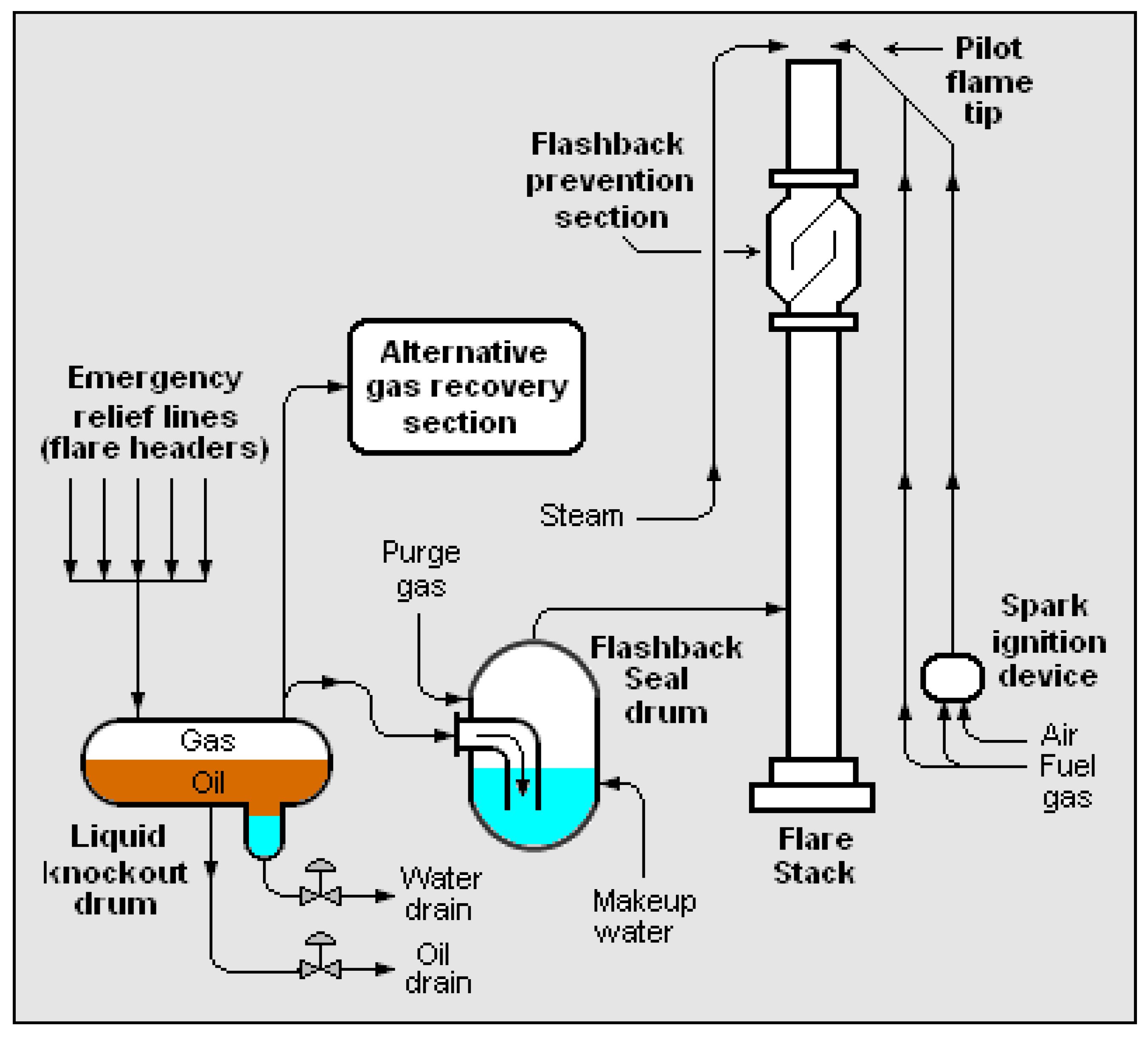
Figure 2.
Computational size and mesh; (a) 65 m (z-axis), 50 m (x-axis) and 50 (y-axis), (b) 75 m (z-axis), 50 m (x-axis) and 50 (y-axis), (c) 85 m (z-axis), 50 m (x-axis) and 50 (y-axis). .
Figure 2.
Computational size and mesh; (a) 65 m (z-axis), 50 m (x-axis) and 50 (y-axis), (b) 75 m (z-axis), 50 m (x-axis) and 50 (y-axis), (c) 85 m (z-axis), 50 m (x-axis) and 50 (y-axis). .
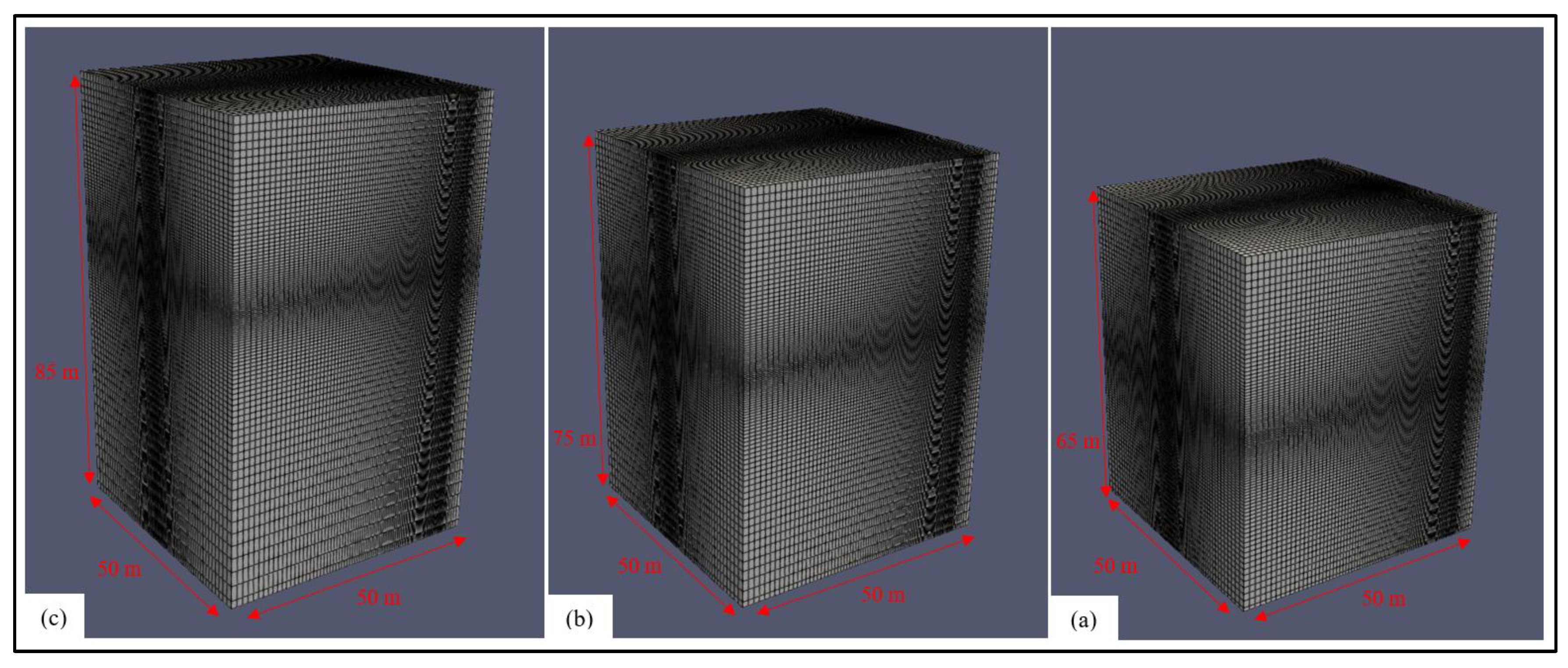
Figure 3.
Flare model and ground mesh; (a) 35 m stack height, (b) 45 m stack height, (c) 55 m stack height.
Figure 3.
Flare model and ground mesh; (a) 35 m stack height, (b) 45 m stack height, (c) 55 m stack height.
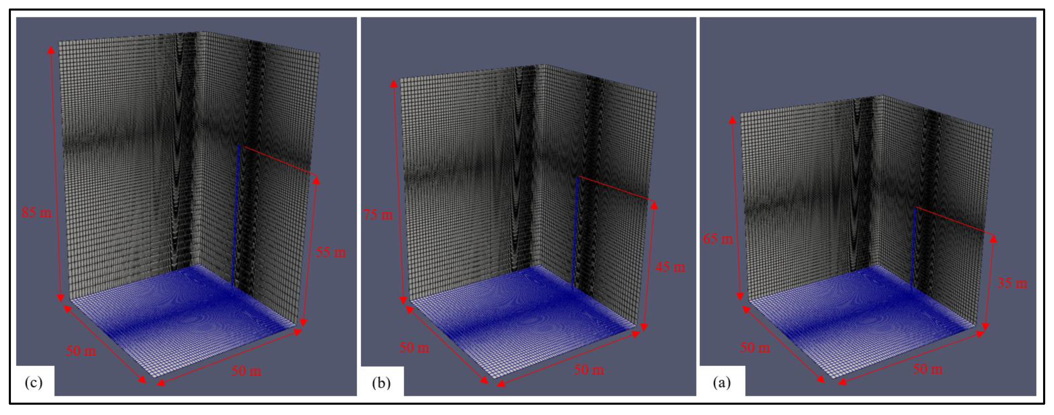
Figure 4.
Data sampling locations for mesh independence study at 9 t/hr firing rate using stack height 55 m; (a) 14 m (x-axis), 0 m (y-axis), 60 m (z-axis), (b) 16 m (x-axis), 0 m (y-axis), 60 m (z-axis), (c) 18 m (x-axis), 0 m (y-axis), 60 m (z-axis), (d) 20 m (x-axis), 0 m (y-axis), 60 m (z-axis).
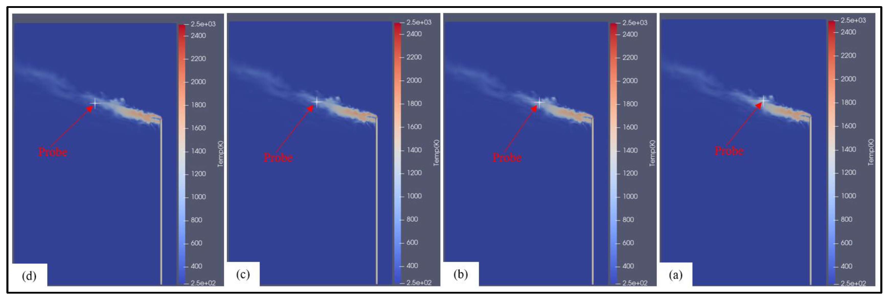
Figure 5.
Data sampling locations for mesh independence study at 9 t/hr firing rate using stack height 45 m; (a) 14 m (x-axis), 0 m (y-axis), 50 m (z-axis), (b) 16 m (x-axis), 0 m (y-axis), 50 m (z-axis), (c) 18 m (x-axis), 0 m (y-axis), 50 m (z-axis), (d) 20 m (x-axis), 0 m (y-axis), 51 m (z-axis).
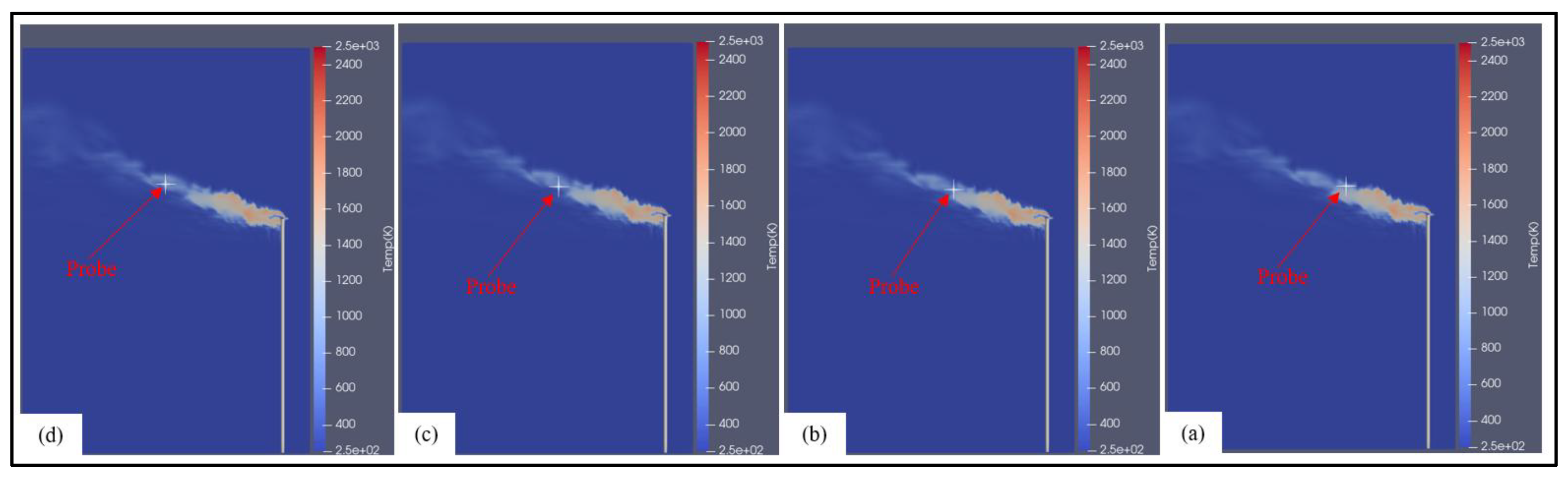
Figure 6.
Data sampling locations for mesh independence study at 9 t/hr firing rate using stack height 35 m; (a) 12 m (x-axis), 0 m (y-axis), 40 m (z-axis), (b) 14 m (x-axis), 0 m (y-axis), 40 m (z-axis), (c) 16 m (x-axis), 0 m (y-axis), 40 m (z-axis), (d) 18 m (x-axis), 0 m (y-axis), 40 m (z-axis).
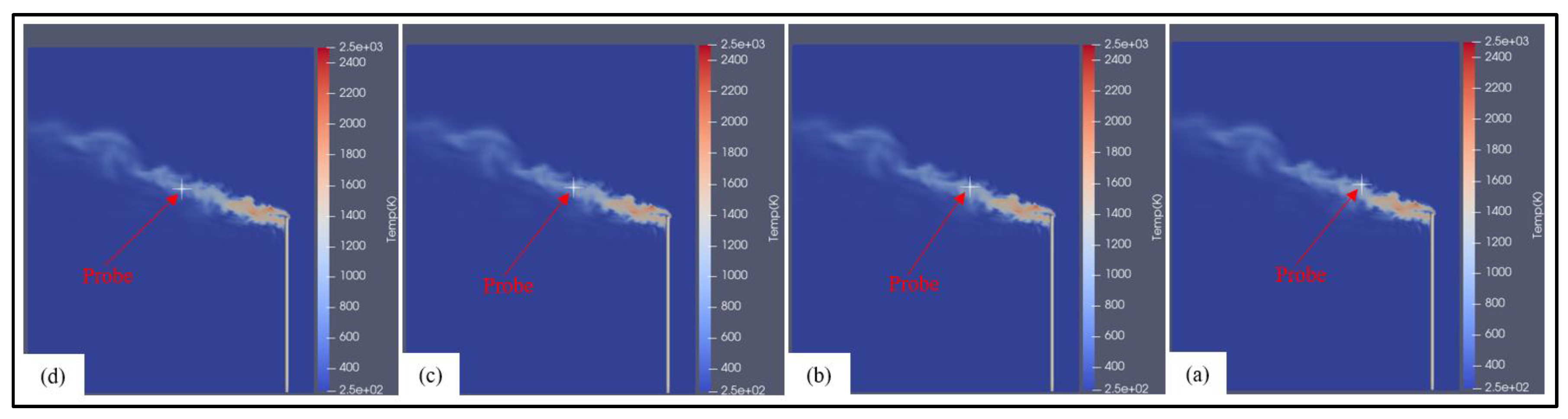
Figure 7.
Mesh independence study for 35 m tall stack case at 9 t/hr firing rate and 8 m/s crosswind.
Figure 7.
Mesh independence study for 35 m tall stack case at 9 t/hr firing rate and 8 m/s crosswind.
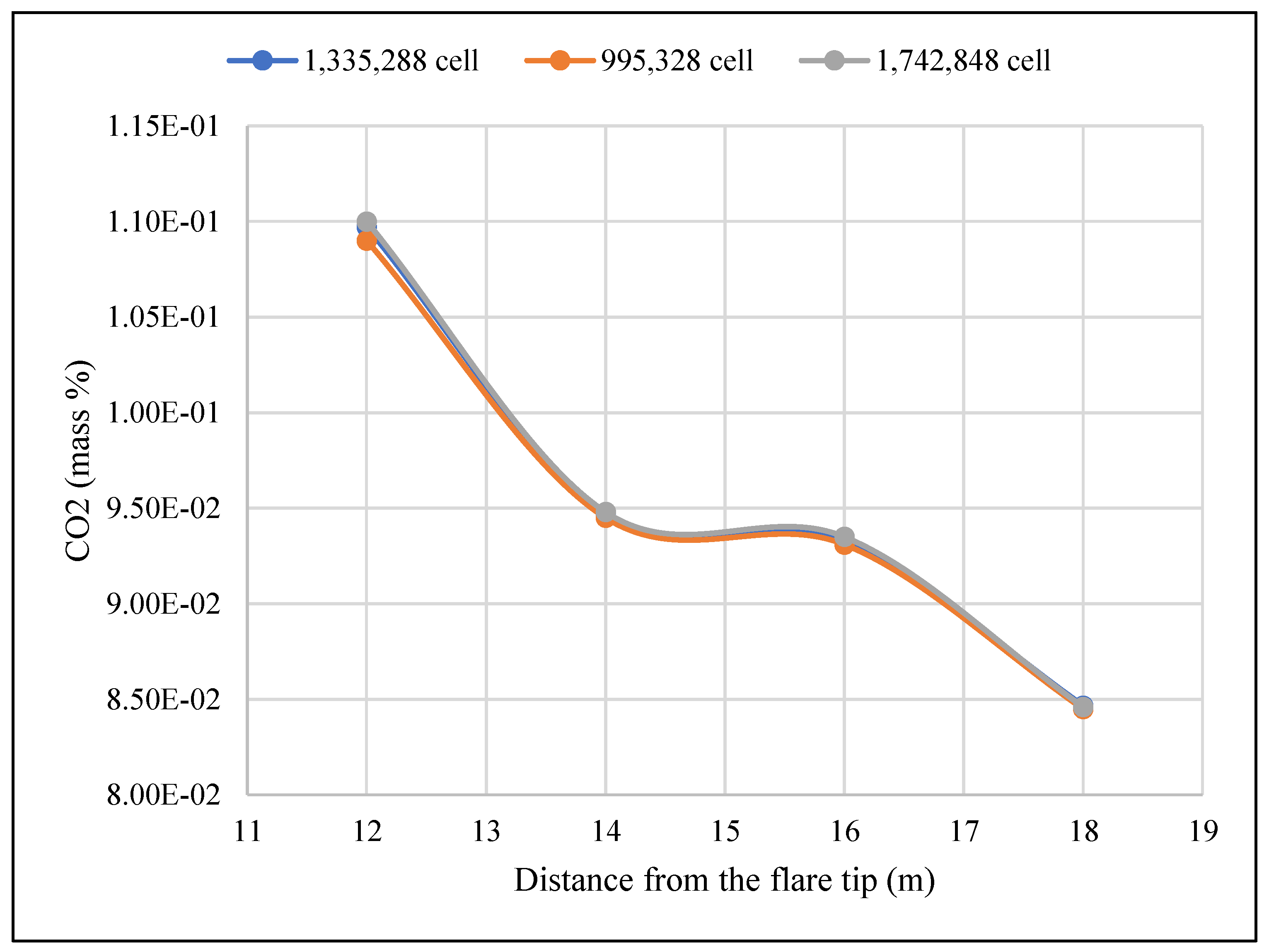
Figure 8.
Mesh independence study for 45 m tall stack case at 9 t/hr firing rate and 8 m/s crosswind.
Figure 8.
Mesh independence study for 45 m tall stack case at 9 t/hr firing rate and 8 m/s crosswind.
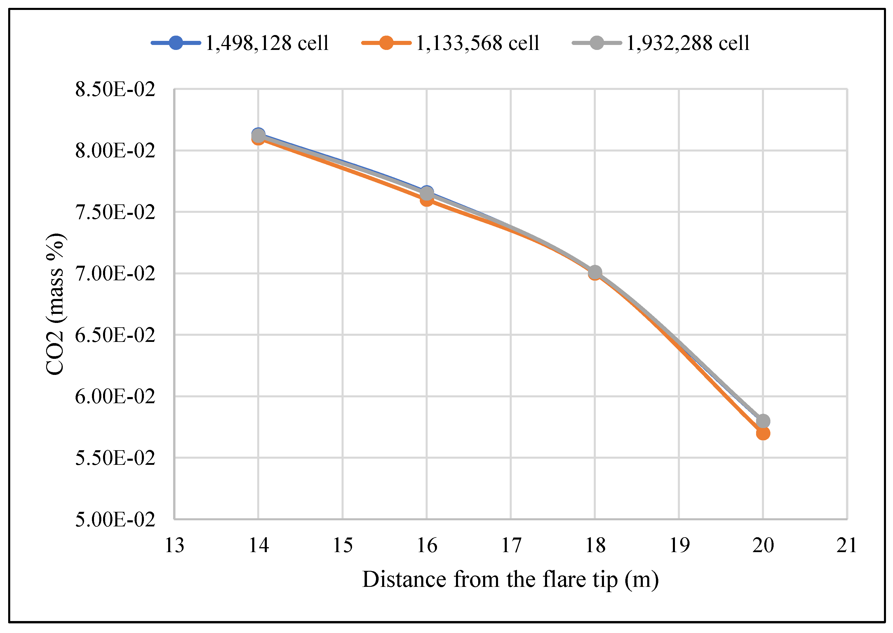
Figure 9.
Mesh independence study for 55 m tall stack case at 9 t/hr firing rate and 8 m/s crosswind.
Figure 9.
Mesh independence study for 55 m tall stack case at 9 t/hr firing rate and 8 m/s crosswind.
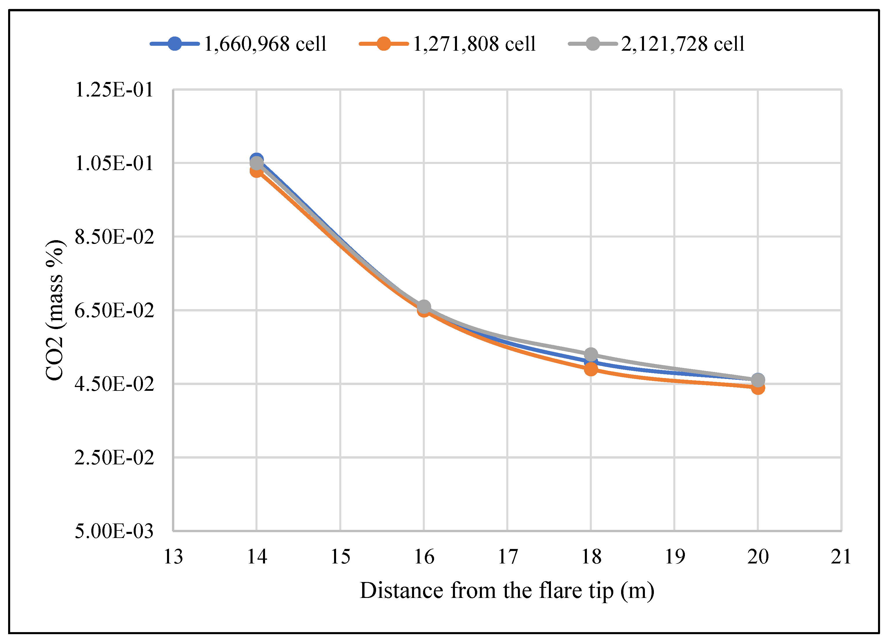
Figure 10.
Net reaction energy source and simulation time step size for 2.5 kg/s gas firing rate cases.
Figure 10.
Net reaction energy source and simulation time step size for 2.5 kg/s gas firing rate cases.
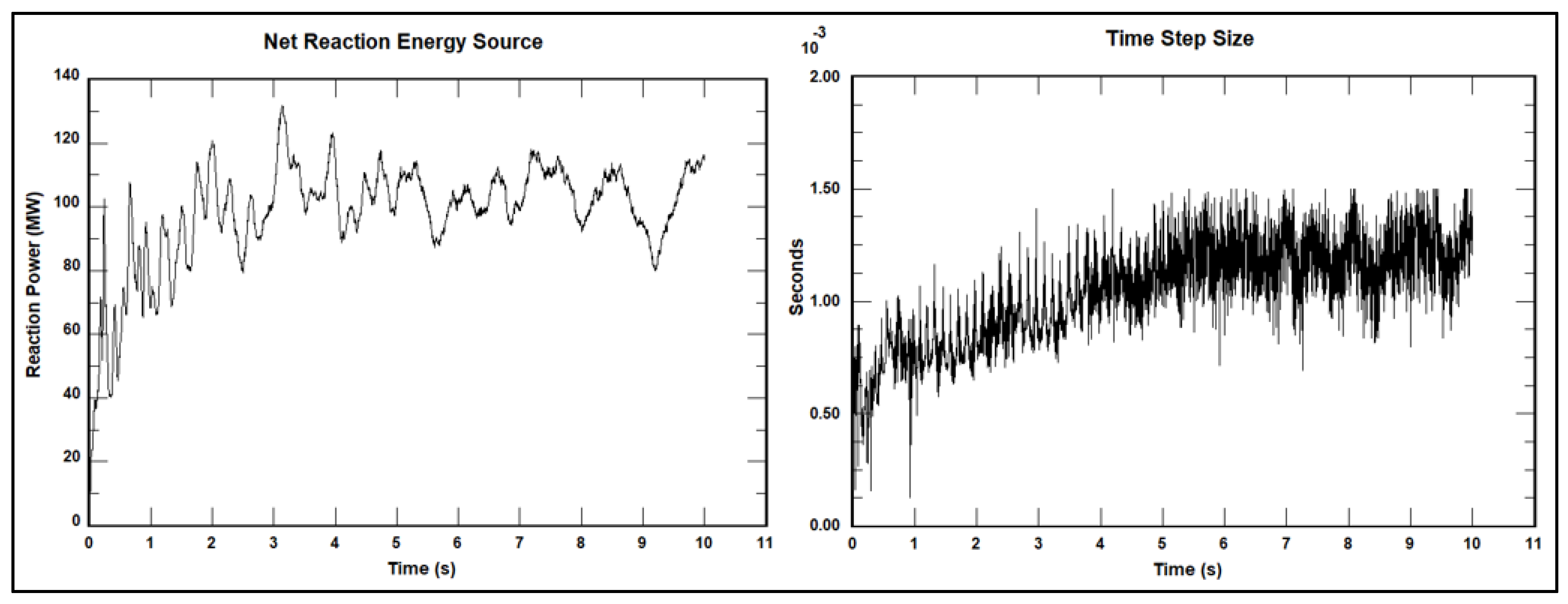
Figure 11.
Net reaction energy source and simulation time step size for 12.5 kg/s gas firing rate cases.
Figure 11.
Net reaction energy source and simulation time step size for 12.5 kg/s gas firing rate cases.
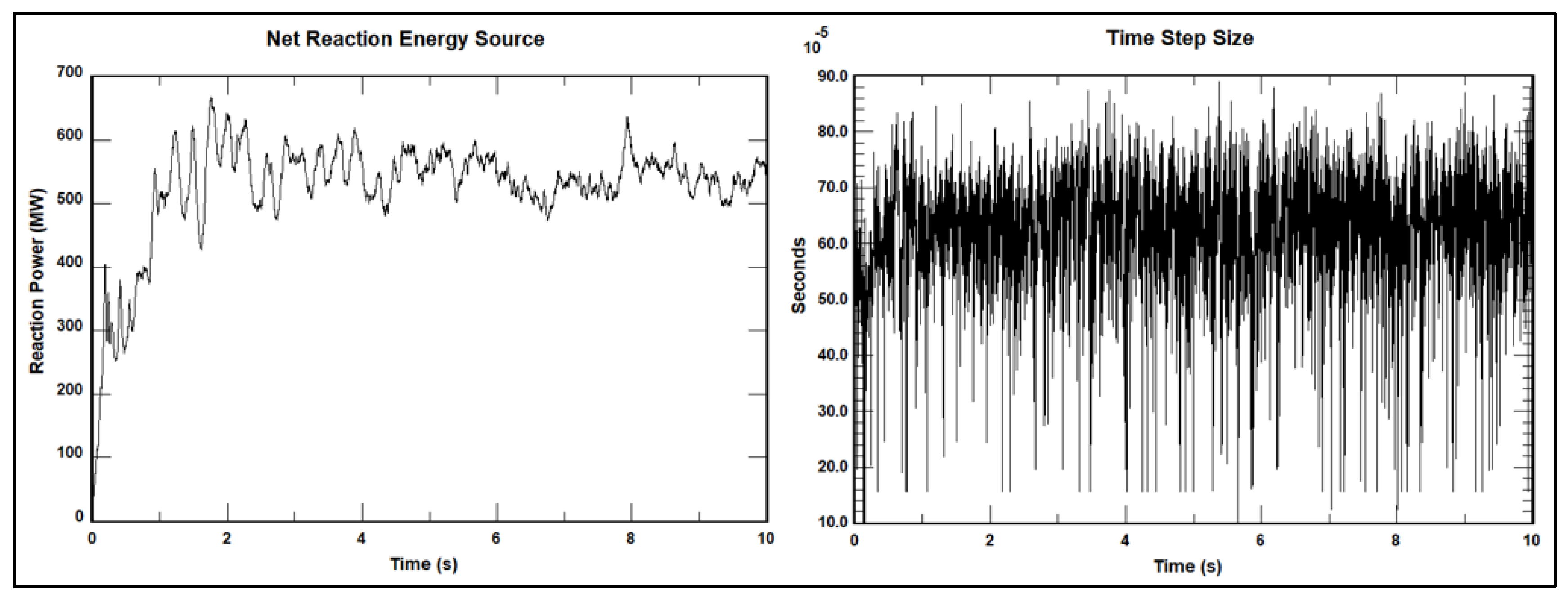
Figure 12.
Low gas firing rate flare operation under three different crosswind speeds: (a) 4 m/s, (b) 8 m/s and (c) 14 m/s.
Figure 12.
Low gas firing rate flare operation under three different crosswind speeds: (a) 4 m/s, (b) 8 m/s and (c) 14 m/s.
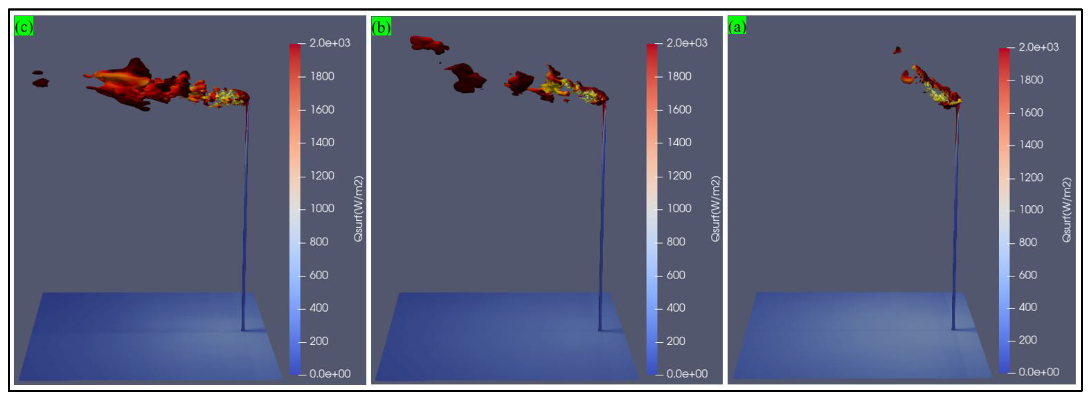
Figure 13.
High gas firing rate flare operation under three different crosswind speeds: (a) 4 m/s, (b) 8 m/s and (c) 14 m/s.
Figure 13.
High gas firing rate flare operation under three different crosswind speeds: (a) 4 m/s, (b) 8 m/s and (c) 14 m/s.
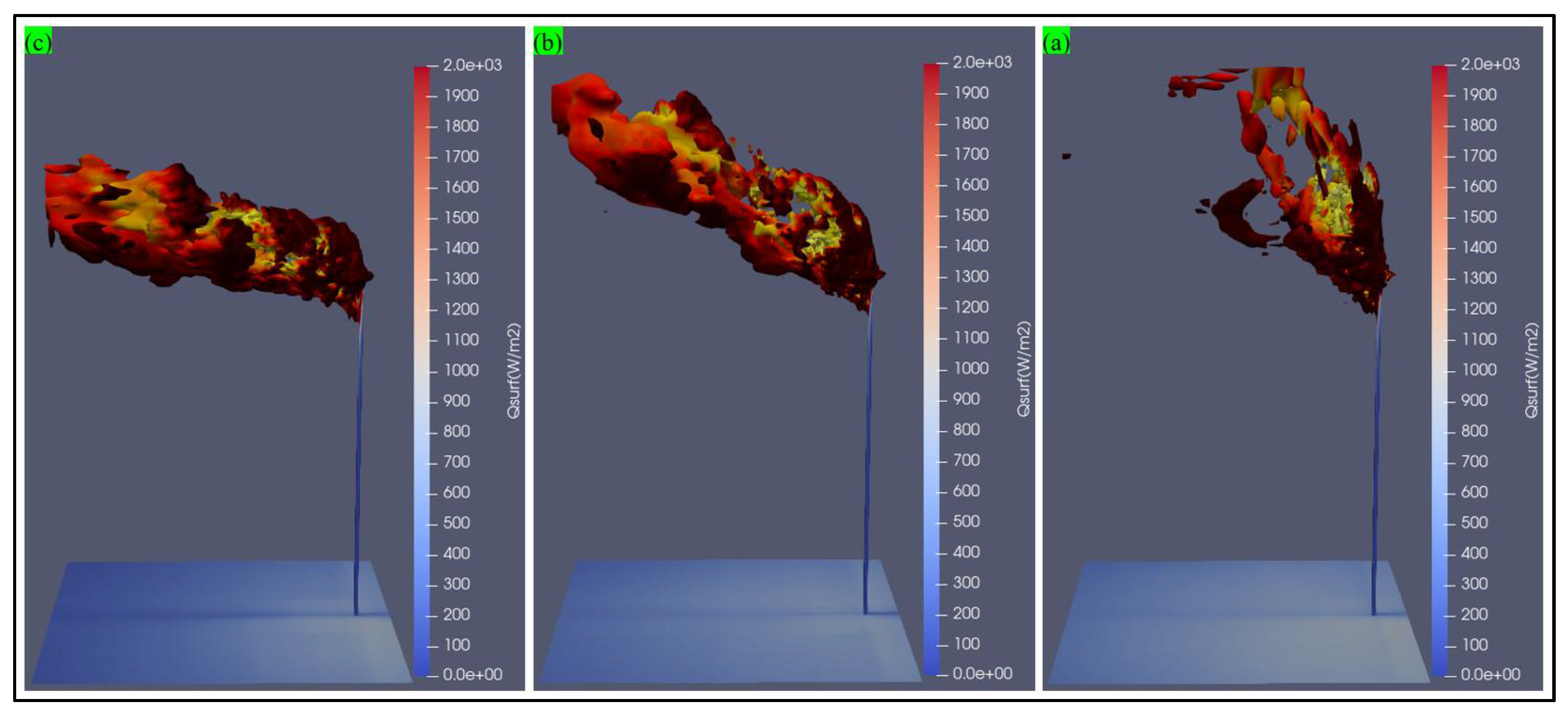
Figure 14.
Flame temperature at a normal gas firing rate under different crosswind speed; (a) 4 m/s, (b) 8 m/s and (c) 14 m/s.
Figure 14.
Flame temperature at a normal gas firing rate under different crosswind speed; (a) 4 m/s, (b) 8 m/s and (c) 14 m/s.
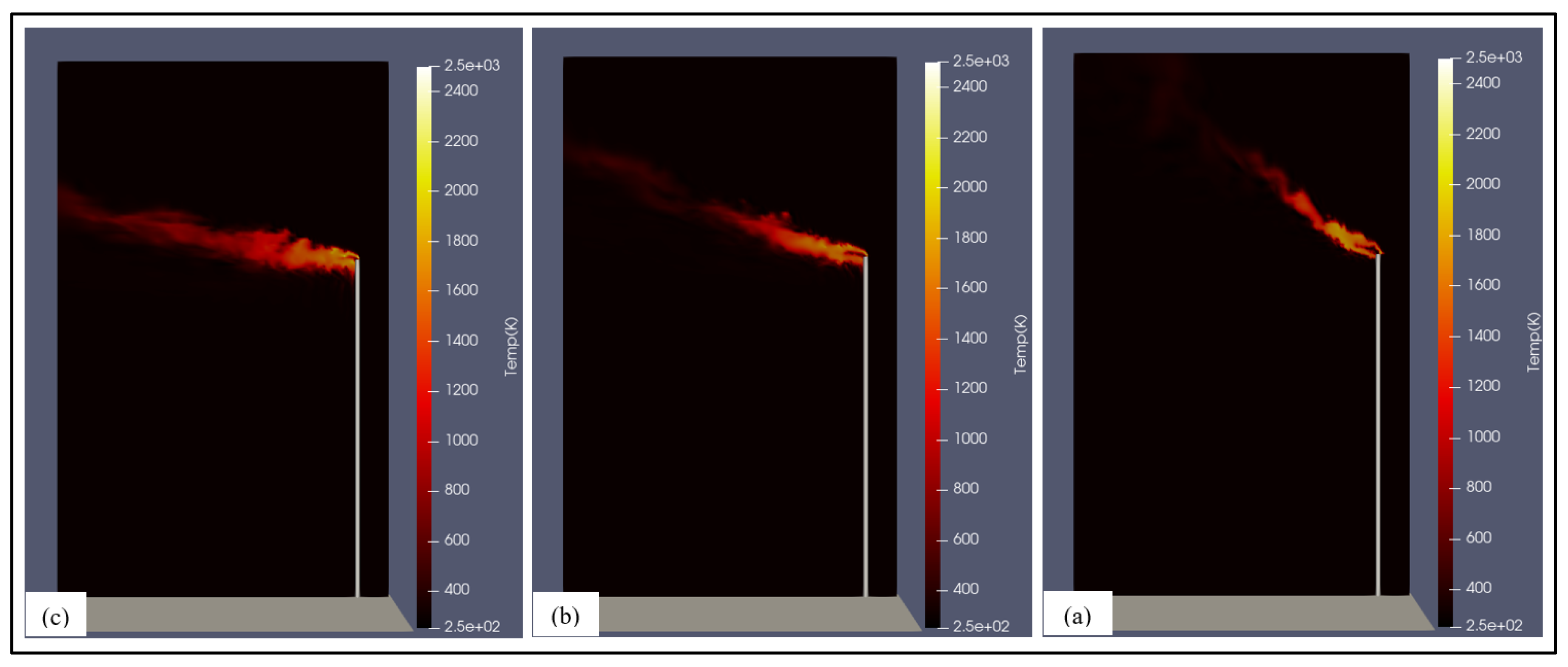
Figure 15.
Flame temperature at a high gas firing rate under different crosswind speed; (a) 4 m/s, (b) 8 m/s and (c) 14 m/s.
Figure 15.
Flame temperature at a high gas firing rate under different crosswind speed; (a) 4 m/s, (b) 8 m/s and (c) 14 m/s.
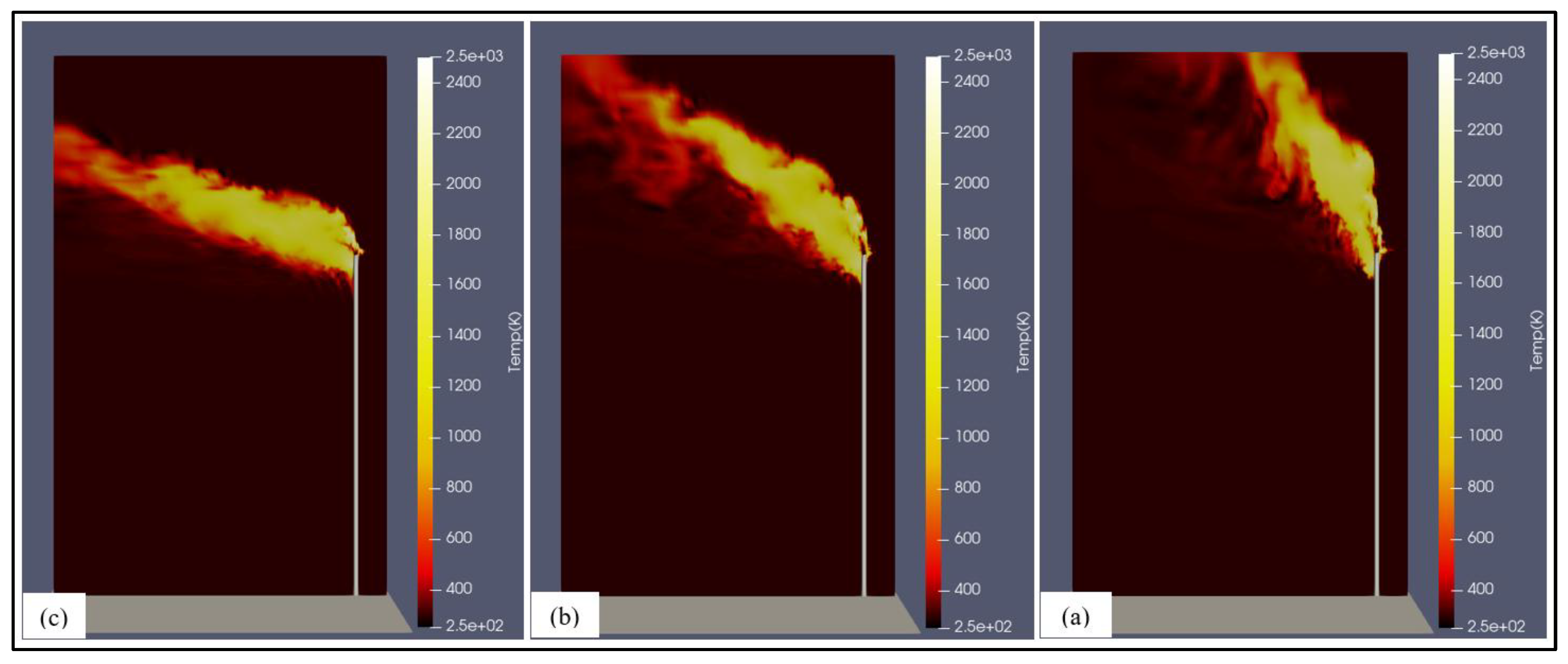
Figure 16.
Soot formation at a normal gas firing rate under different crosswind speed; (a) 4 m/s, (b) 8 m/s and (c) 14 m/s.
Figure 16.
Soot formation at a normal gas firing rate under different crosswind speed; (a) 4 m/s, (b) 8 m/s and (c) 14 m/s.
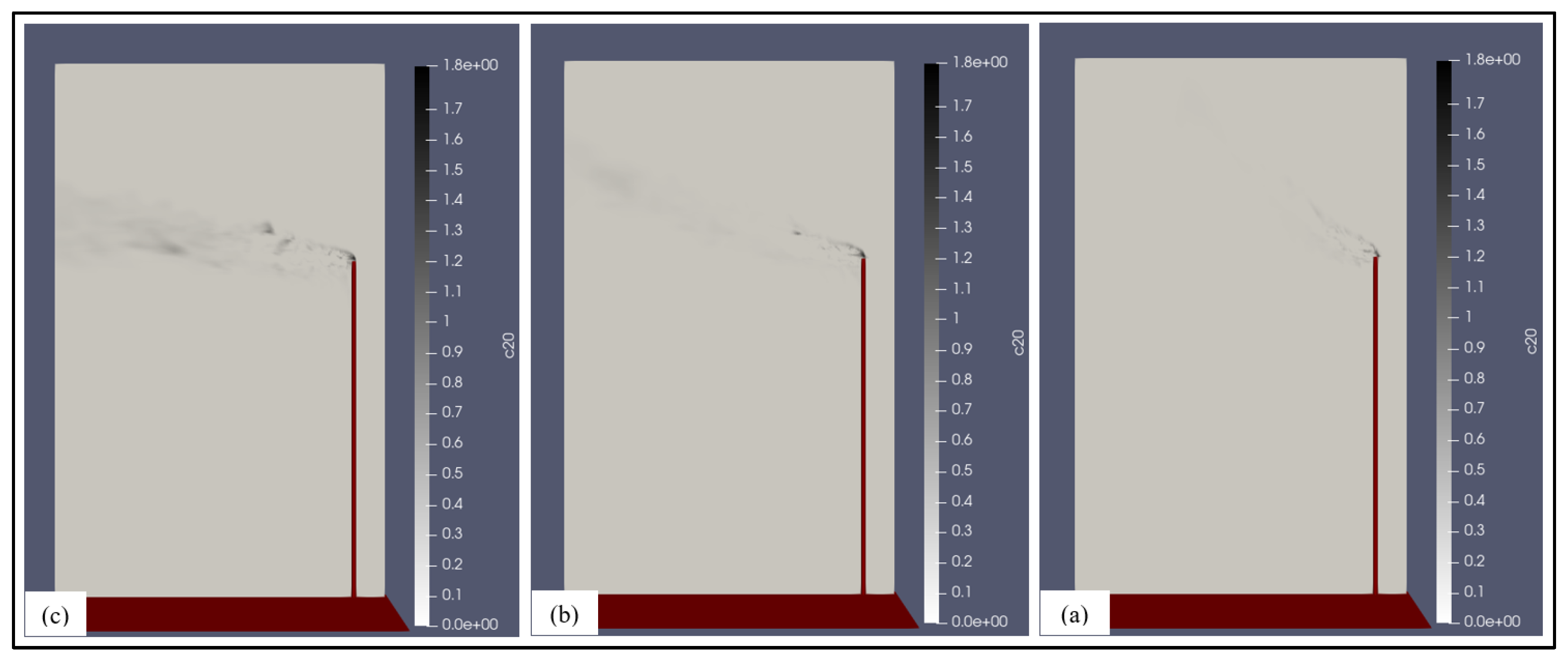
Figure 17.
Soot formation at a high gas firing rate under different crosswind speed; (a) 4 m/s, (b) 8 m/s and (c) 14 m/s.
Figure 17.
Soot formation at a high gas firing rate under different crosswind speed; (a) 4 m/s, (b) 8 m/s and (c) 14 m/s.
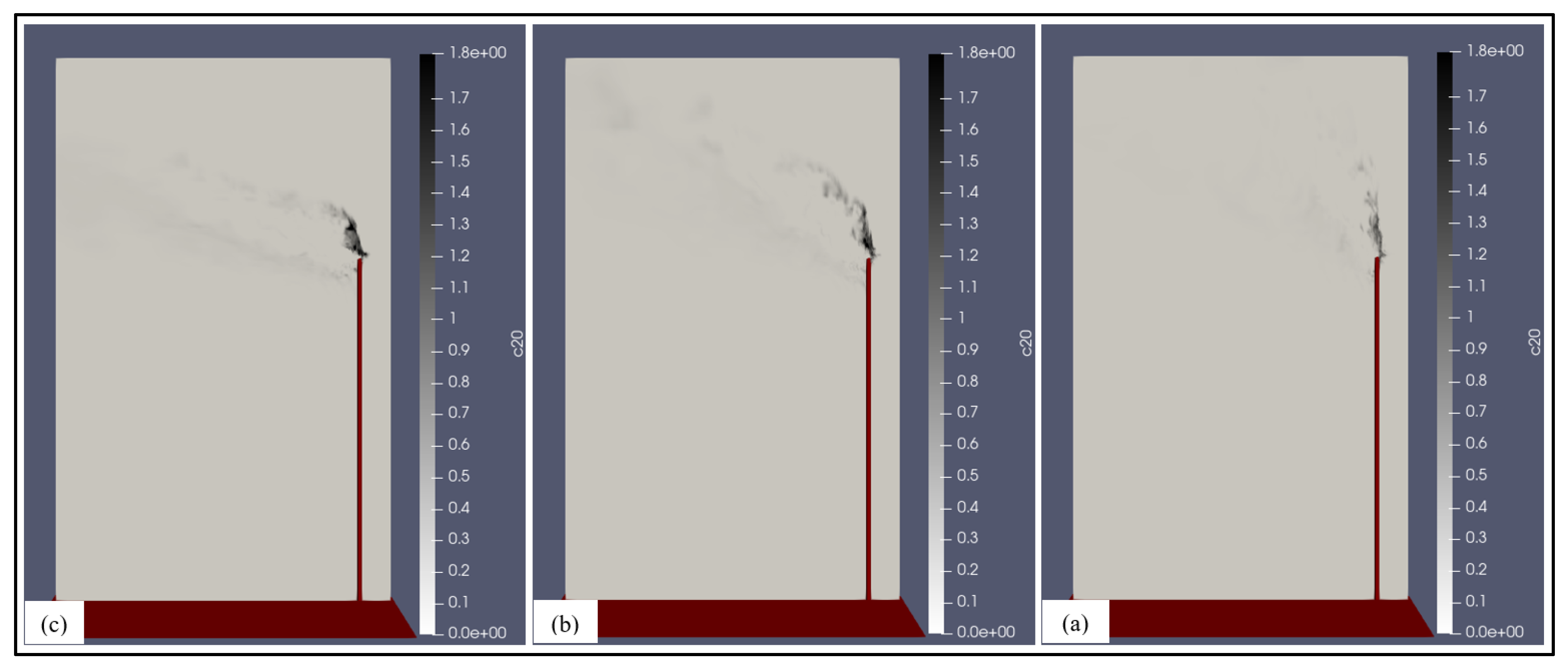
Figure 18.
Carbon dioxide emissions at a normal gas firing rate under different crosswind speed; (a) 4 m/s, (b) 8 m/s and (c) 14 m/s.
Figure 18.
Carbon dioxide emissions at a normal gas firing rate under different crosswind speed; (a) 4 m/s, (b) 8 m/s and (c) 14 m/s.
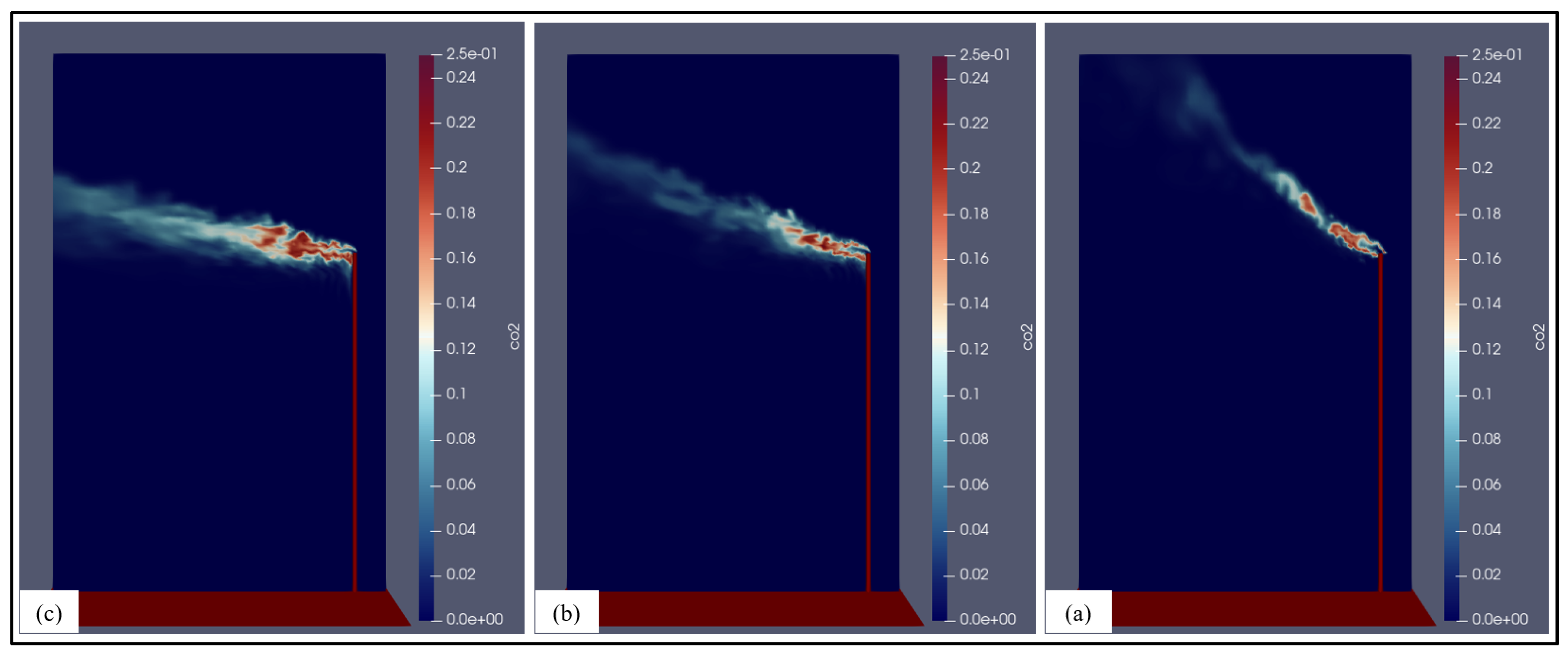
Figure 19.
Carbon dioxide emissions at a high gas firing rate under different crosswind speed; (a) 4 m/s, (b) 8 m/s and (c) 14 m/s.
Figure 19.
Carbon dioxide emissions at a high gas firing rate under different crosswind speed; (a) 4 m/s, (b) 8 m/s and (c) 14 m/s.
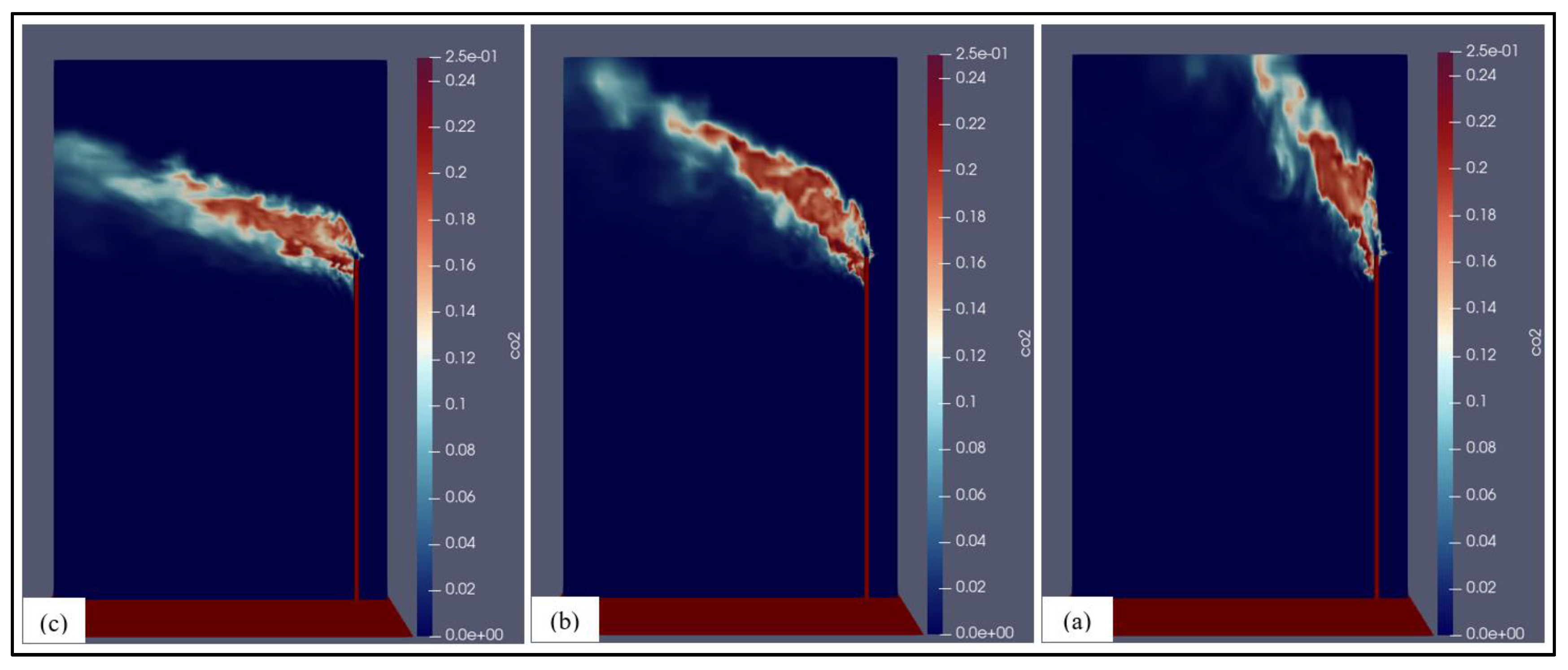
Figure 20.
Carbon monoxide emissions at a normal gas firing rate under different crosswind speed; (a) 4 m/s, (b) 8 m/s and (c) 14 m/s.
Figure 20.
Carbon monoxide emissions at a normal gas firing rate under different crosswind speed; (a) 4 m/s, (b) 8 m/s and (c) 14 m/s.
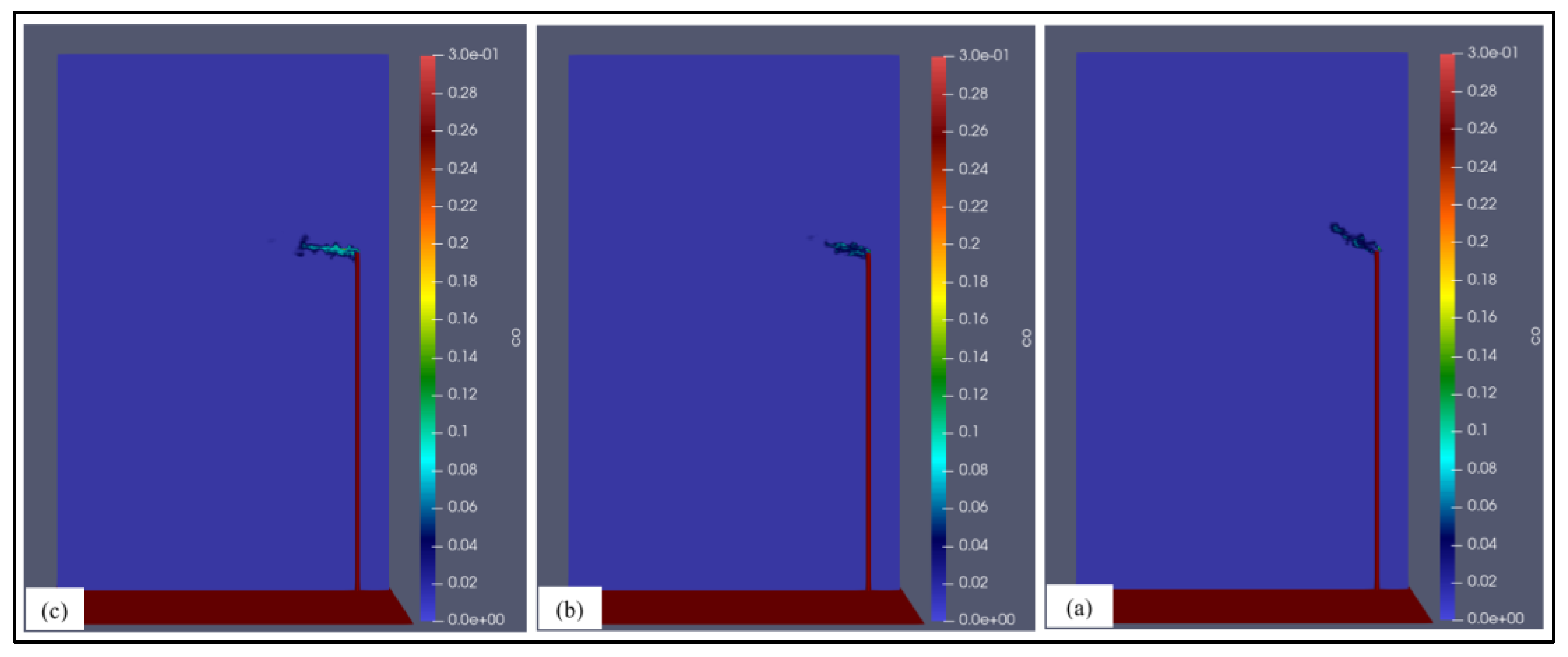
Figure 21.
Carbon monoxide emissions at a high gas firing rate under different crosswind speed; (a) 4 m/s, (b) 8 m/s and (c) 14 m/s.
Figure 21.
Carbon monoxide emissions at a high gas firing rate under different crosswind speed; (a) 4 m/s, (b) 8 m/s and (c) 14 m/s.
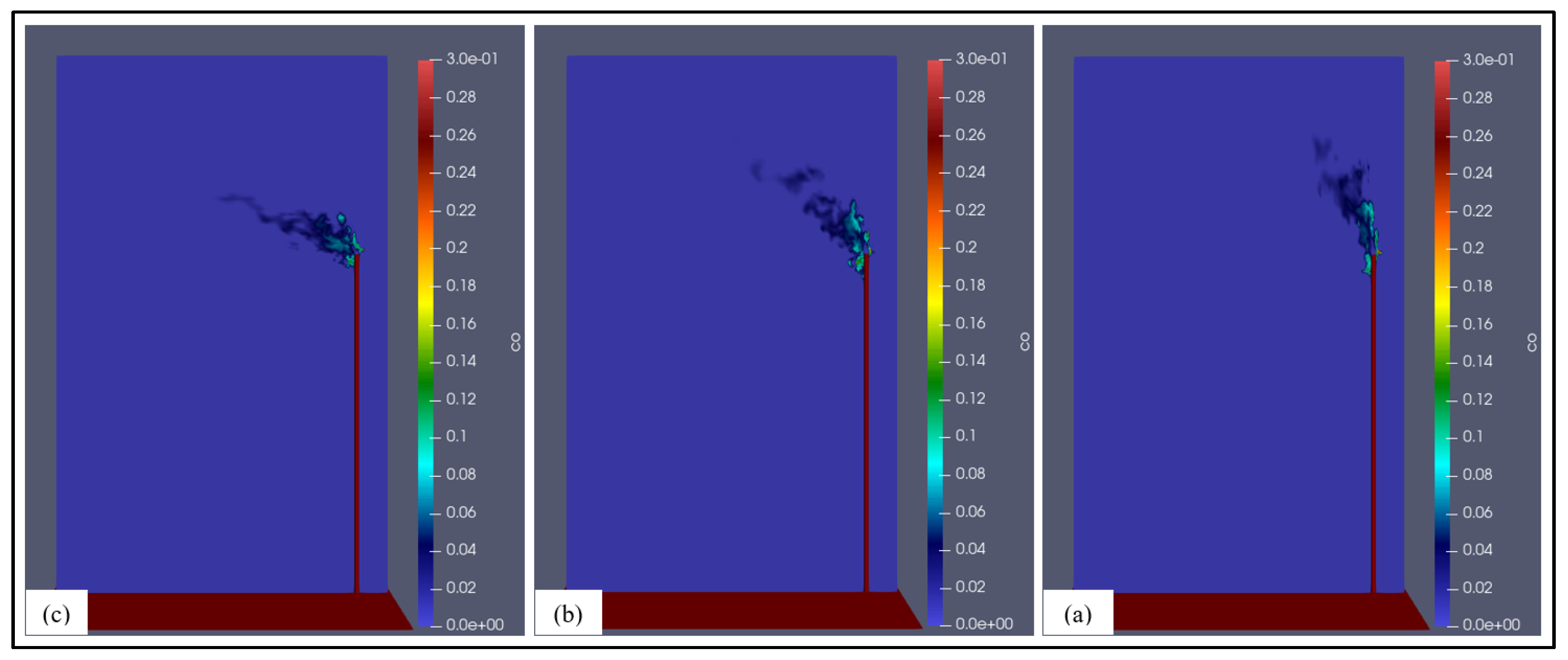
Figure 22.
Sulphur dioxide emissions at a normal gas firing rate under different crosswind speed; (a) 4 m/s, (b) 8 m/s and (c) 14 m/s.
Figure 22.
Sulphur dioxide emissions at a normal gas firing rate under different crosswind speed; (a) 4 m/s, (b) 8 m/s and (c) 14 m/s.
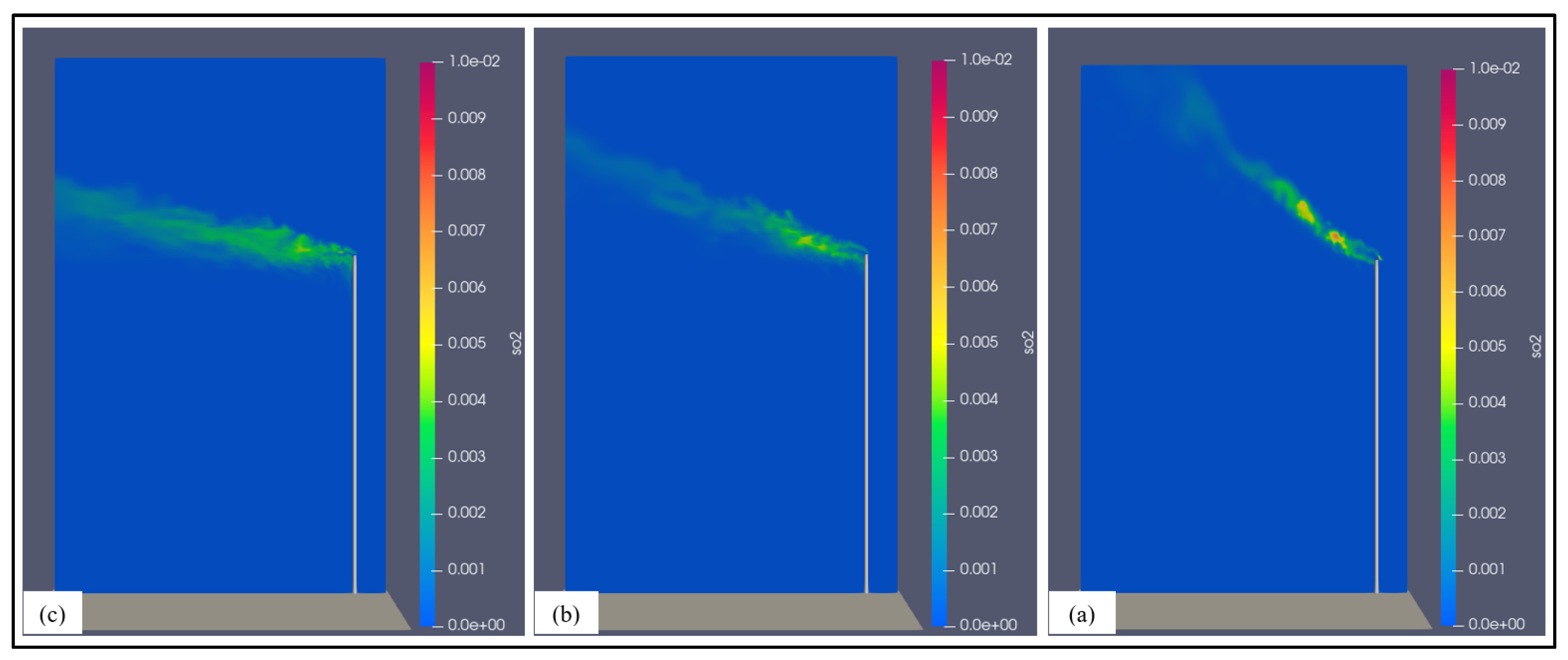
Figure 23.
Sulphur dioxide emissions at a normal gas firing rate under different crosswind speed; (a) 4 m/s, (b) 8 m/s and (c) 14 m/s.
Figure 23.
Sulphur dioxide emissions at a normal gas firing rate under different crosswind speed; (a) 4 m/s, (b) 8 m/s and (c) 14 m/s.
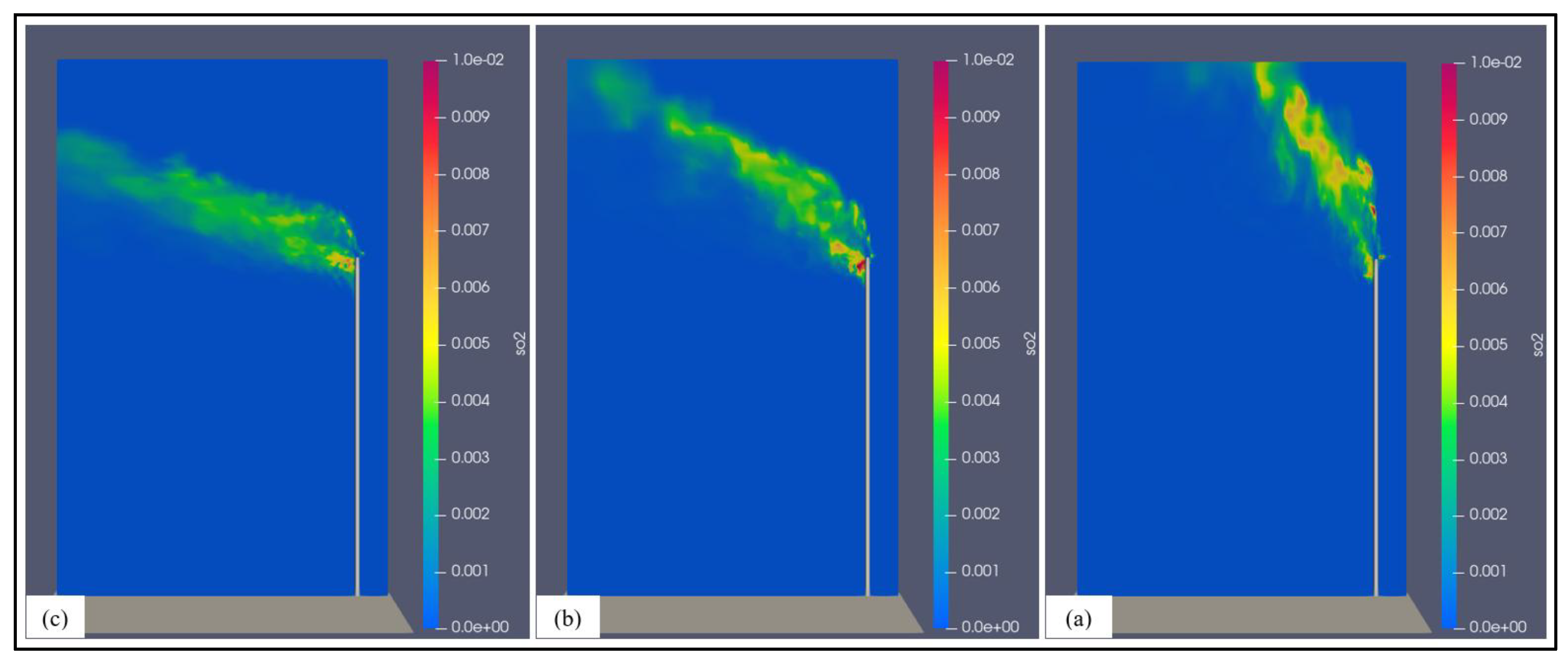
Figure 24.
Nitric oxide emissions at a normal gas firing rate under different crosswind speed; (a) 4 m/s, (b) 8 m/s and (c) 14 m/s.
Figure 24.
Nitric oxide emissions at a normal gas firing rate under different crosswind speed; (a) 4 m/s, (b) 8 m/s and (c) 14 m/s.
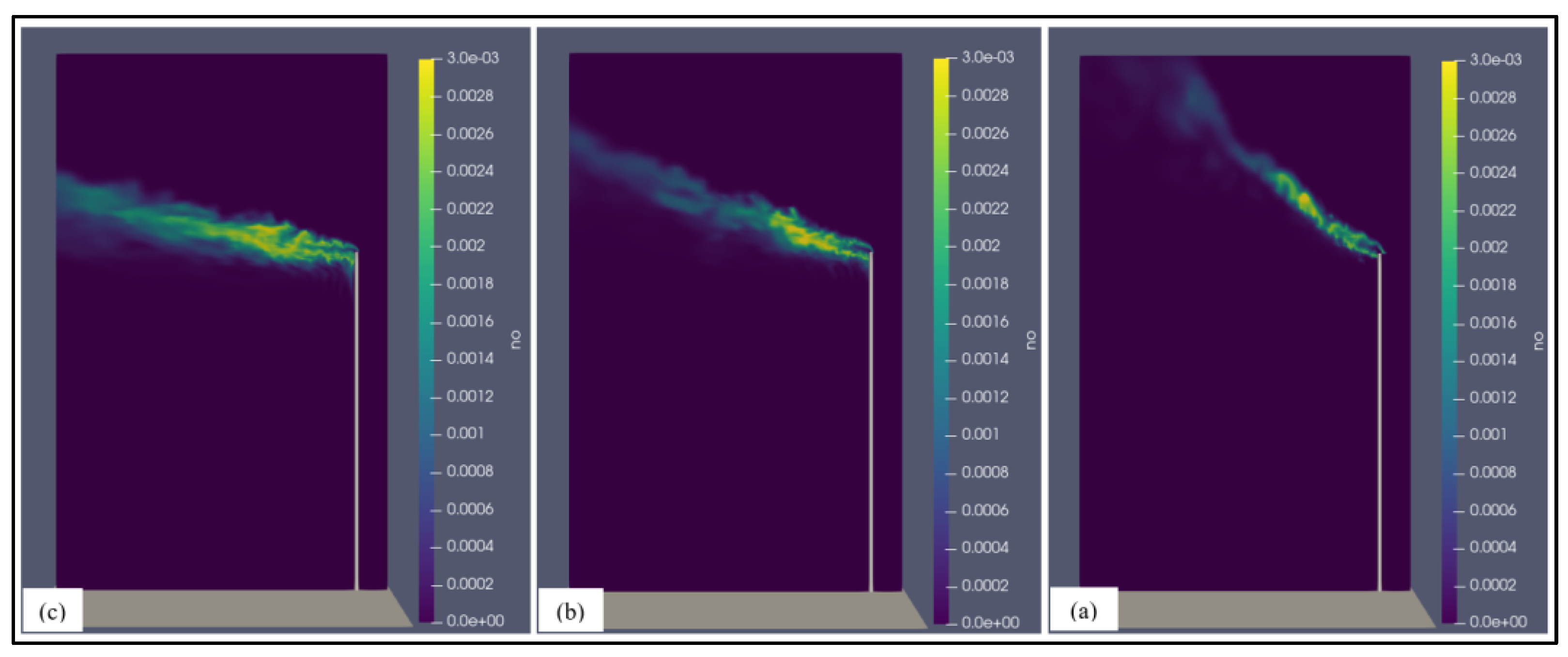
Figure 25.
Nitric oxide emissions at a high gas firing rate under different crosswind speed; (a) 4 m/s, (b) 8 m/s and (c) 14 m/s.
Figure 25.
Nitric oxide emissions at a high gas firing rate under different crosswind speed; (a) 4 m/s, (b) 8 m/s and (c) 14 m/s.
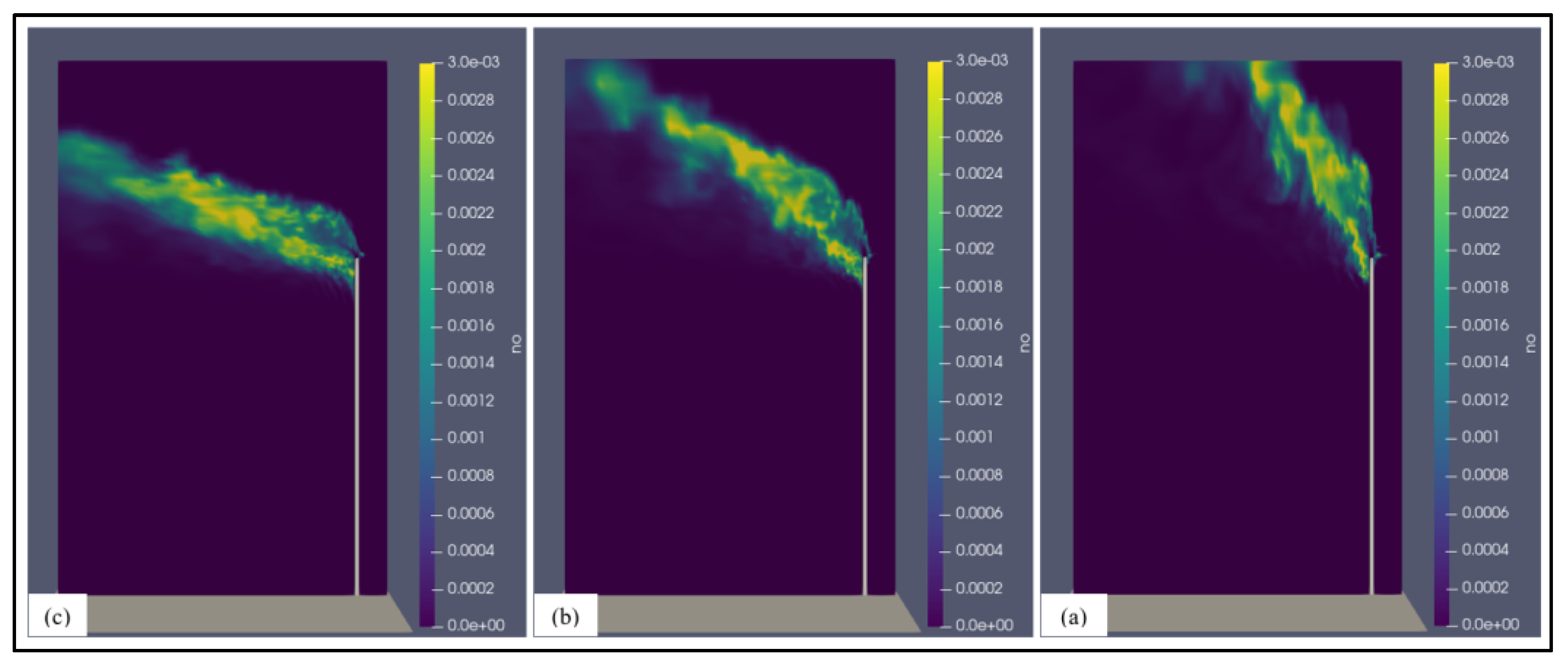
Figure 26.
Low gas firing rate flare operation using three different stack heights: (a) 55 m, (b) 45 m and (c) 35 m.
Figure 26.
Low gas firing rate flare operation using three different stack heights: (a) 55 m, (b) 45 m and (c) 35 m.
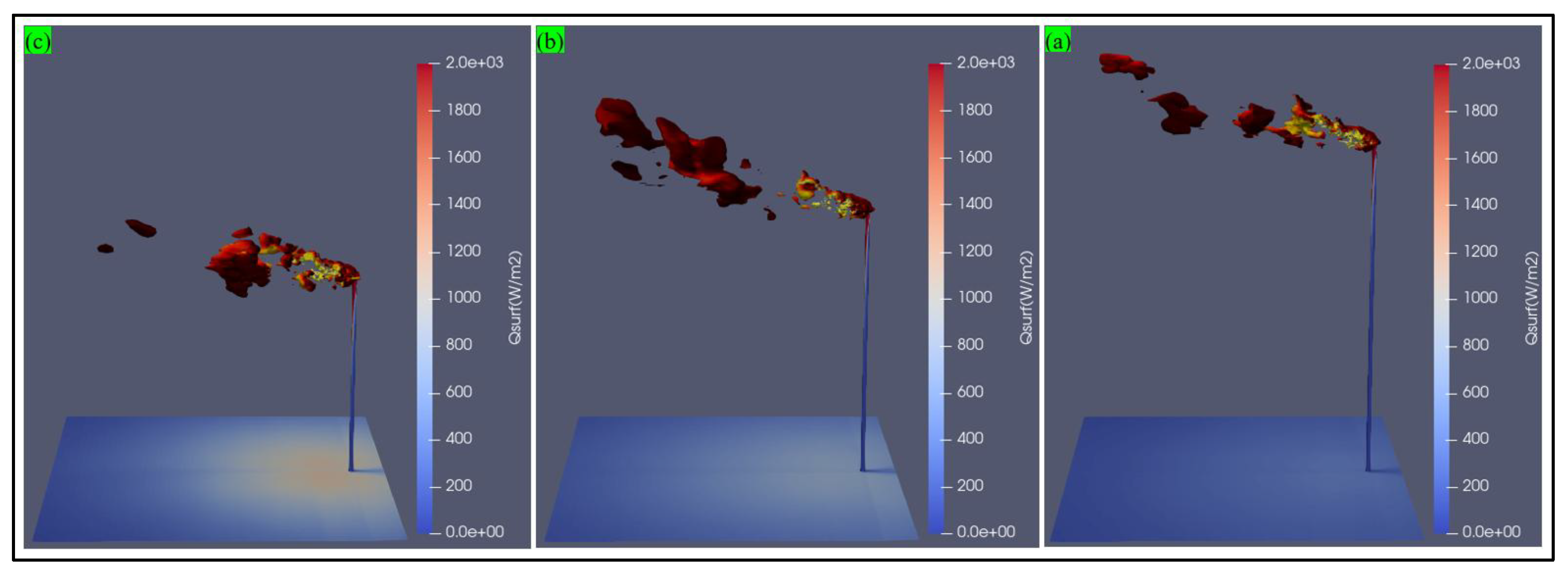
Figure 27.
High gas firing rate flare operation using three different stack heights: (a) 55 m, (b) 45 m and (c) 35 m.
Figure 27.
High gas firing rate flare operation using three different stack heights: (a) 55 m, (b) 45 m and (c) 35 m.
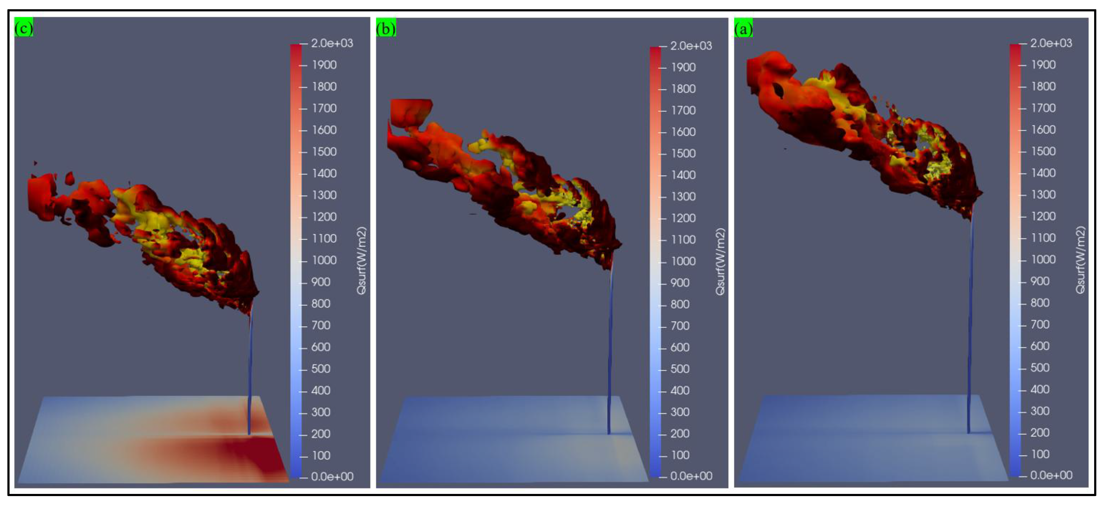
Figure 28.
Probe locations at normal gas firing rate of the flare using stack height of 55 m; (a) 14 m (x-axis), 0 m (y-axis), 60 m (z-axis), (b) 16 m (x-axis), 0 m (y-axis), 60 m (z-axis), (c) 18 m (x-axis), 0 m (y-axis), 60 m (z-axis), (d) 20 m (x-axis), 0 m (y-axis), 60 m (z-axis)..
Figure 28.
Probe locations at normal gas firing rate of the flare using stack height of 55 m; (a) 14 m (x-axis), 0 m (y-axis), 60 m (z-axis), (b) 16 m (x-axis), 0 m (y-axis), 60 m (z-axis), (c) 18 m (x-axis), 0 m (y-axis), 60 m (z-axis), (d) 20 m (x-axis), 0 m (y-axis), 60 m (z-axis)..
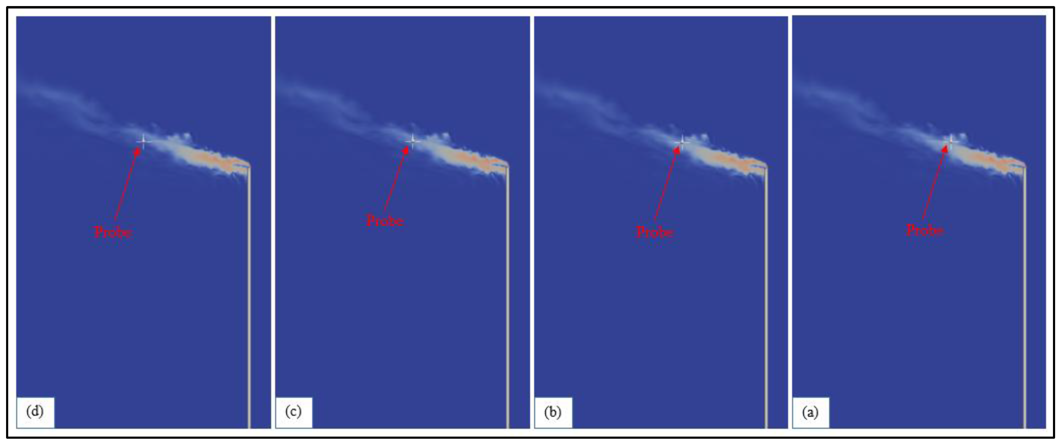
Figure 29.
Probe locations at high gas firing rate of the flare using stack height 55 m; ; (a) 25 m (x-axis), 0 m (y-axis), 74 m (z-axis), (b) 27 m (x-axis), 0 m (y-axis), 74 m (z-axis), (c) 29 m (x-axis), 0 m (y-axis), 74 m (z-axis), (d) 30 m (x-axis), 0 m (y-axis), 75 m (z-axis)..
Figure 29.
Probe locations at high gas firing rate of the flare using stack height 55 m; ; (a) 25 m (x-axis), 0 m (y-axis), 74 m (z-axis), (b) 27 m (x-axis), 0 m (y-axis), 74 m (z-axis), (c) 29 m (x-axis), 0 m (y-axis), 74 m (z-axis), (d) 30 m (x-axis), 0 m (y-axis), 75 m (z-axis)..
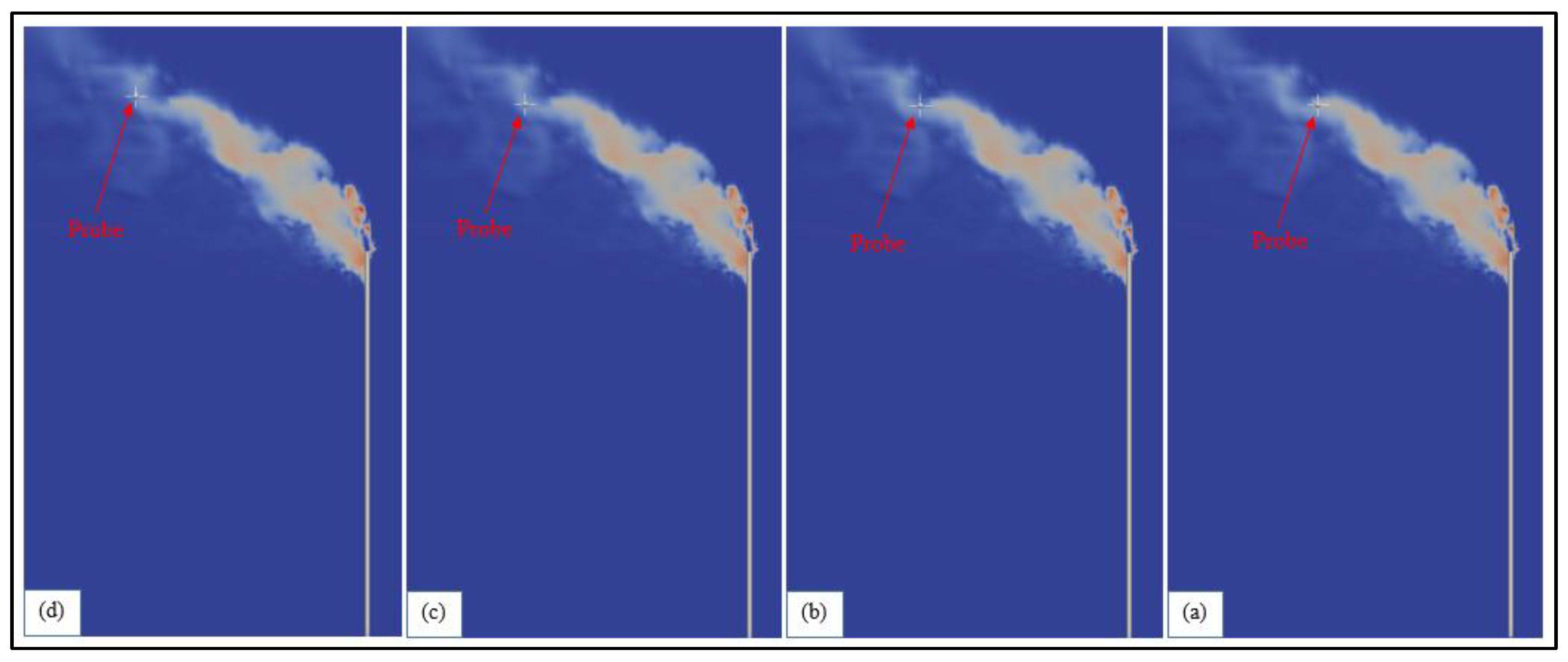

Table 1.
Case study flared gas composition.
| Basis = 100 kg mole | |||||
|---|---|---|---|---|---|
| Components | Mole (%) | Mole (kg mole) | MWt (kg/kg mole) | Mass (kg) | Mass (%) |
| CH4 | 16.44 | 16.44 | 16 | 263.0 | 0.074 |
| C2H6 | 8.80 | 8.80 | 30 | 264.0 | 0.074 |
| C3H8 | 12.5 | 12.5 | 44 | 550.0 | 0.155 |
| C4H10 | 20.35 | 20.35 | 58 | 1180.3 | 0.333 |
| C5H12 | 14.37 | 14.37 | 72 | 1034.6 | 0.292 |
| H2S | 2.96 | 2.96 | 34 | 100.6 | 0.028 |
| H2 | 20.58 | 20.58 | 2 | 41.2 | 0.012 |
| N2 | 4.00 | 4.00 | 28 | 112.0 | 0.032 |
| Total | 100 | 100.0 | 3545.8 | 1.00 | |
Table 2.
Main combustion products at normal gas firing rate.
| Probe Location | CO (Mass%) | CO2 (Mass%) | Soot (Mass%) | SO2 (Mass%) | NO (Mass%) | |||
|---|---|---|---|---|---|---|---|---|
| x-axis (m) | y-axis (m) | z-axis (m) | Radius (m) | |||||
| 14 | 0 | 60 | 0.3 | 6.31E-09 | 1.06E-01 | 1.90E-04 | 2.49E-03 | 2.33E-03 |
| 16 | 0 | 60 | 0.3 | 3.26E-07 | 6.58E-02 | 9.90E-05 | 1.60E-03 | 1.47E-03 |
| 18 | 0 | 60 | 0.3 | 4.52E-09 | 5.10E-02 | 1.42E-04 | 1.22E-03 | 1.14E-03 |
| 20 | 0 | 60 | 0.3 | 1.28E-06 | 4.61E-02 | 2.51E-04 | 1.11E-03 | 1.02E-03 |
Table 3.
Main fuel compounds in the plume during normal gas firing rate.
| Probe Location | CH4 (Mass%) | C2H6 (Mass%) | C3H8 (Mass%) | C4H10 (Mass%) | C5H12 (Mass%) | |||
|---|---|---|---|---|---|---|---|---|
| x-axis (m) | y-axis (m) | z-axis (m) | Radius (m) | |||||
| 14 | 0 | 60 | 0.3 | 8.43E-09 | 7.42E-09 | 7.51E-09 | 7.63E-09 | 7.59E-09 |
| 16 | 0 | 60 | 0.3 | 7.83E-09 | 6.04E-09 | 6.14E-09 | 6.32E-09 | 6.31E-09 |
| 18 | 0 | 60 | 0.3 | 7.80E-09 | 5.30E-09 | 5.41E-09 | 5.62E-09 | 5.62E-09 |
| 20 | 0 | 60 | 0.3 | 6.96E-09 | 4.72E-09 | 4.83E-09 | 5.01E-09 | 5.00E-09 |
Table 4.
Main combustion products at high gas firing rate.
| Probe Location | CO (Mass%) | CO2 (Mass%) | Soot (Mass%) | SO2 (Mass%) | NO (Mass%) | |||
|---|---|---|---|---|---|---|---|---|
| x-axis (m) | y-axis (m) | z-axis (m) | Radius (m) | |||||
| 25 | 0 | 74 | 0.3 | 1.45E-05 | 1.24E-01 | 1.76E-05 | 3.39E-03 | 2.39E-03 |
| 27 | 0 | 74 | 0.3 | 1.16E-08 | 1.38E-01 | 7.06E-05 | 3.91E-03 | 2.76E-03 |
| 29 | 0 | 74 | 0.3 | 2.66E-08 | 1.27E-01 | 3.82E-05 | 3.82E-03 | 2.67E-03 |
| 30 | 0 | 75 | 0.3 | 2.83E-07 | 7.78E-02 | 1.05E-04 | 2.27E-03 | 1.67E-03 |
Table 5.
Main fuel compounds in the plume during high gas firing rate.
| Probe Location | CH4 (Mass%) | C2H6 (Mass%) | C3H8 (Mass%) | C4H10 (Mass%) | C5H12 (Mass%) | |||
|---|---|---|---|---|---|---|---|---|
| x-axis (m) | y-axis (m) | z-axis (m) | Radius (m) | |||||
| 25 | 0 | 74 | 0.3 | 7.59E-08 | 1.04E-06 | 1.61E-06 | 4.93E-06 | 4.38E-06 |
| 27 | 0 | 74 | 0.3 | 9.47E-09 | 9.60E-09 | 9.52E-09 | 9.83E-09 | 9.69E-09 |
| 29 | 0 | 74 | 0.3 | 9.06E-09 | 8.39E-09 | 8.44E-09 | 8.59E-09 | 8.68E-09 |
| 30 | 0 | 75 | 0.3 | 8.69E-09 | 6.29E-09 | 6.40E-09 | 6.60E-09 | 6.59E-09 |
Table 6.
Main flare gas compounds in the fuel and the plume during normal gas firing rate.
| Plume | |||||||||||
| Probe Location | CH4 (Mass%) | C2H6 (Mass%) | C3H8 (Mass%) | C4H10 (Mass%) | C5H12 (Mass%) | ||||||
| x-axis (m) | y-axis (m) | z-axis (m) | Radius (m) | ||||||||
| 14 | 0 | 60 | 0.3 | 8.43E-09 | 7.42E-09 | 7.51E-09 | 7.63E-09 | 7.59E-09 | |||
| 16 | 0 | 60 | 0.3 | 7.83E-09 | 6.04E-09 | 6.14E-09 | 6.32E-09 | 6.31E-09 | |||
| 18 | 0 | 60 | 0.3 | 7.80E-09 | 5.30E-09 | 5.41E-09 | 5.62E-09 | 5.62E-09 | |||
| 20 | 0 | 60 | 0.3 | 6.96E-09 | 4.72E-09 | 4.83E-09 | 5.01E-09 | 5.00E-09 | |||
| Fuel | 7.40E-02 | 7.40E-02 | 1.55E-01 | 3.33E-01 | 2.92E-01 | ||||||
Table 7.
Main flare gas compounds in the fuel and the plume during high gas firing rate.
| Plume | ||||||||
| Probe Location | CH4 (Mass%) | C2H6 (Mass%) | C3H8 (Mass%) | C4H10 (Mass%) | C5H12 (Mass%) | |||
| x-axis (m) | y-axis (m) | z-axis (m) | Radius (m) | |||||
| 14 | 0 | 60 | 0.3 | 7.59E-08 | 1.04E-06 | 1.61E-06 | 4.93E-06 | 4.38E-06 |
| 16 | 0 | 60 | 0.3 | 9.47E-09 | 9.60E-09 | 9.52E-09 | 9.83E-09 | 9.69E-09 |
| 18 | 0 | 60 | 0.3 | 9.06E-09 | 8.39E-09 | 8.44E-09 | 8.59E-09 | 8.68E-09 |
| 20 | 0 | 60 | 0.3 | 8.69E-09 | 6.29E-09 | 6.40E-09 | 6.60E-09 | 6.59E-09 |
| Fuel | 7.40E-02 | 7.40E-02 | 1.55E-01 | 3.33E-01 | 2.92E-01 | |||
Disclaimer/Publisher’s Note: The statements, opinions and data contained in all publications are solely those of the individual author(s) and contributor(s) and not of MDPI and/or the editor(s). MDPI and/or the editor(s) disclaim responsibility for any injury to people or property resulting from any ideas, methods, instructions or products referred to in the content. |
© 2025 by the authors. Licensee MDPI, Basel, Switzerland. This article is an open access article distributed under the terms and conditions of the Creative Commons Attribution (CC BY) license (http://creativecommons.org/licenses/by/4.0/).
Copyright: This open access article is published under a Creative Commons CC BY 4.0 license, which permit the free download, distribution, and reuse, provided that the author and preprint are cited in any reuse.


