
Submitted:
23 January 2025
Posted:
26 January 2025
You are already at the latest version
Abstract
Carbonate - open-water mangroves have high OC content, apparently due to sediments’ biophysical characteristics. However, the role of key regulators such as salinity and hydroperiod, which modulate the forest structure and therefore carbon dynamics, has been little explored. This study evaluates the influence of salinity on the accumulation of aerial and underground OC (production of litter and roots), in open-water karstic forests. For this purpose, an experimental design was implemented on San Andrés Island, where there is an edaphic salinity gradient because of the water regime. Three physiographic types of mangroves characterized by different saline regimes were selected. Two inland forests of mesohaline regime (9.63 ± 6.26 and 11.54 ± 7.46 PSU), a euhaline fringe forest (37.47 ± 5.76 PSU), and a hyperhaline regime basin forest (62.36 ± 10.54 PSU). The working hypothesis was the existence of an inverse relationship between salinity and litter production, and a direct relationship between salinity and root production. Root production was evaluated using the growth core implantation technique (108 soil cores), selecting live roots according to diameter (<2, 2-5 and 5-20 mm). The mean (±SD) OC content in dry litter (Mg C ha-1 y-1) was 8.96 ± 0.28; 5.57 ± 0.15; 6.31 ± 0.27; and 4.54 ± 0.8; while the production of dry roots was 0.41 ± 0.08; 1.19 ± 0.46; 1.30 ± 0.5 and 0.24 ± 0.20, for the mesohaline forests, the euhaline forest and the hyperhaline forest, respectively. The proposed hypothesis was sustained among forests with marked salinity ranges. Leaf litter production was not very high in forests with intermediate salinity, and root production was very low in high salinity, suggesting that salinity acts in synergy with other variables influencing the species composition and their functioning. These results affirm the high productivity of carbonate environments and the contribution of autochthonous production.
Keywords:
mangrove
; blue carbon
; root production
; litter production
; salinity
1. Introduction
Mangrove forests are strategic ecosystems located at the sea-land interface, with special morphological, physiological, and reproductive adaptations that allow them to dominate in environments with wide fluctuations in flooding and soil salinity [1]. In addition to providing important ecosystem services such as coastal protection and fishery and forestry supplies [2] mangroves, along with seagrasses and salt marshes, are recognized for the ability to retain large amounts of organic carbon (OC) [3], which constitutes an important climate change mitigation mechanism.
Values of OC recorded in biomass and underground in mangrove forests (853 Mg C ha–1, [4]), are double those reported in tropical forests (400 Mg C ha–1) and quadruple those of temperate forests (220 Mg C ha –1, [5]).The capacity of mangroves to absorb atmospheric CO2 depends on factors such as density and forest productivity, basal area, height, and age of the trees, as well as the photosynthetic efficiency of each species [6] .These factors are influenced by the physicochemical characteristics of water and soil (e.g., pH, redox potential, salinity and nutrients), topography [7], hydroperiod, sediment dynamics and climate [8].This is why the capacity of mangroves to sequester carbon varies widely at the global, regional, and local levels [9].
Forest biomass and sediments constitute the main OC reservoirs in mangrove forests. The former (aerial carbon) represents a short-term deposit, while the latter (underground carbon) is a long-term deposit [10].Most studies have focused on quantifying these reservoirs, leaving gaps in information on the processes or flows of OC between reservoirs, which is important for forest management. Underground reserves constitute about 85% of the total OC content of mangrove forests [4]. This is the result of the accumulation of both autochthonous and allochthonous organic matter, along with the high production of underground roots and the efficient recycling of nutrients, which generate unique biomass production and allocation processes [4,11].
Carbon (C) distribution between forest reservoirs depends largely on the hydrological regime. In terrigenous environments that receive autochthonous and allochthonous materials through river flow and with sediments characterized by low salinity, reduced N:P ratio, and frequent flooding [12], more C is allocated to the aerial biomass than to the roots [13]. However, in carbonate environments without river discharges in which sediment accumulation is autochthonous, and phosphorus (P) tends to be a limiting factor [14], greater biomass is allocated to the roots, increasing the concentration of C in these sediments [15].
Although there are numerous studies on mangrove leaf litter fall, few address variability due to saline stress [16,17]. Interannual climate events such as El Niño and La Niña - Southern Oscillation (ENSO) strongly affect precipitation regimes [18], also altering salinity. Periods of intense drought or strong floods can have serious impacts, mainly on karstic and deltaic mangroves [19].
Root production has been quantified in various investigations (e.g. [13,20,21,22] .For the most part, fine roots are those with the greatest contribution in the first 30 cm of the soil with 66% of the total root production [21,23,24,25], Likewise, it has been found that root dynamics are not explained solely by the concentration of nutrients in the soil, but that the interaction between the hydroperiod (frequency and duration) and edaphic regulators (salinity, sulfides, Eh) also intervenes [13].
The forests of San Andrés, an oceanic island of karstic origin and lacking rivers [6,13,26] , provide the opportunity to examine the influence of salinity and the hydrological regime in the flows and accumulation of OC in different physiographic types of mangroves. To address this objective, we proposed the existence of an inverse relationship between salinity and litter production, and a direct relationship between salinity and root production as a working hypothesis.
2. Materials and Methods
2.1. Study Area
San Andrés Island, located in the southwest of the Caribbean between 12°29' and 12°36' N latitude and 81°41' and 81°43' W longitude at 619 km from the Colombian coasts, has 27 km2 and is part of the Archipelago of San Andrés, Providencia and Santa Catalina and the Seaflower Biosphere Reserve [13]. It has a warm-humid climate with an average annual temperature of 27.4°C, maximums between 29 and 30°C (May to June) and minimums between 25.5 and 26.0°C (December to February). The average annual precipitation is 1797.8 mm, unevenly distributed between a dry season (January to April) influenced by trade winds and a wet season (October to December), with approximately 80% of the annual precipitation [27] .There are no permanent surface water currents on the island. However, during the rainy season, high flows of runoff are formed, which quickly disappear within a few hours as the aquifers are recharged [28]
The marine-coastal environment of the island favors the development of mangroves. In these areas, the lithology presents deposits of calcareous sands and gravel composed of coral fragments. The decomposition of vegetation on residual soils generates layers of peat and organic clay, leading to the formation of sand, clay, and peat deposits. These deposits are distributed in several sectors near the eastern coast of the island, with an average thickness of approximately 2 [28]
The selected forests are in Old Point Mangrove Regional Park (PRMOP), Sound Bay and Smith Channel. The PRMOP, located in the northeast of the island (12°33'96” N, 81°42' 51”W), presents a fringe mangrove forest dominated by Rhizophora mangle, followed by Avicennia germinans and Laguncularia racemosa. The ground elevation in this area varies from 0.23 to 0.3 m (mean sea level, MSL), with the mangroves being influenced by precipitation and semi-diurnal tides with an average amplitude of ~32 cm [29], which regulate interstitial salinity (<35 PSU; [6]).
In PRMOP, a basin forest also develops, whose water contribution is governed by semidiurnal tides and climate which, added to the topographic characterization, makes its salinity higher (> 50 PSU; [6]), due in part to the ground elevation, which is lower in this type of forest (decreasing from 0.20 m MSL in the north to −0.20 m MSL in the south of the forest), as well as the presence of a formation of ridges with higher elevation on the southeastern side of the forest that restricts the exchange of water with the ocean. Poor drainage conditions and permanent flooding during spring tides are observed at this site [13].
On the southwest side of San Andrés Island there are two inland forests, Sound Bay and Smith Channel (14.4 and 18.1 ha, respectively). These forests do not have a direct connection with the sea because the presence of a sand dune prevents the contact of the forest with this body of water; the water supply for these sites is provided by rain and indirectly by groundwater. There are no sources of fresh water such as rivers or streams [30]. During the rainy season these forests remain flooded and water loss is due to evaporation [13]. The elevation of the ground in these forests varies from 0 to 2.5 m MSL in less than 20 m from the coast due to the presence of the dune and decreases to 0.7 m MSL towards the interior of the forest Medina Calderón, 2016. The salinity is < 10 practical salinity units (PSU) throughout the year [6,13,32].The maximum flood level is recorded in October with 34.2 cm, while the lowest levels of the water table are observed especially in April (drier) [31].
According to the Venice system [33], hydrological environments can be classified according to their salinity range into limnetic systems (< 0.5 PSU), oligohaline (0.5 to 5 PSU), mesohaline (5 to 18 PSU), polyhaline (18 to 30 PSU), euhaline (30 to 40 PSU) and hyperhaline (> 40 PSU). Following this classification, the mangrove forests of San Andrés Island can be considered hyperhaline (basin forest in Hooker Bay), euhaline (fringe forest in Hooker Bay) and mesohaline (inland forests in Smith Channel and Sound Bay).
2.2. Experiment Design
From January 2012 to 2019 a total of 14 plots (20 x 20 m) were established in the basin and fringe forests of the PRMOP (hereinafter named BHC and BHF, respectively) and in the inland forest within Smith Channel (SCTA) (a description of the plots installation can be found in [13]). For the Sound Bay Inland Forest (SBTA) four permanent plots of 20 x 20 m were established from January to December 2022. The plots were considered as experimental units and treated as replicates within each forest. The forests were structurally characterized, the carbon content of root and leaf litter production was estimated, and the salinity of the interstitial water and the relationship with climatic variables such as precipitation, temperature, and wind speed were measured.
2.2.1. Forest Structure
In each plot (3 BHC, 5 BHF, 4 SBTA and 6 SCTA), all trees with DBH greater than 2.5 cm were measured, as well as the species composition, tree density (trees ha-1), the basal area (m2 ha-1) and the Importance Value Index (IVI).
2.2.2. Leaf Litter Production
From 2012 to 2019 (BHC, BHF and SCTA) and in 2022 (SBTA), litter production was measured monthly. In each plot, five baskets of 0.25 m2 (N=20) made of PVC with a 0.3 mm mesh bottom were randomly placed at a height of 1 m. The fallen leaf litter was collected every month, and the collected material was dried in an oven at 60 °C for 72 hours, then separated into four categories: leaves (leaves and stipules), reproductive structures (flowers, fruits and propagules), wood (bark and branches), and remains (uncategorized plant material). This material was weighed on a semi-analytical balance (Ohaus scout pro with 0.01 g precision). The results were expressed in g m-2 y-1. Dry biomass was converted to C using a conversion factor of 0.5 [34], and results were expressed Mg C ha-1 y-1.
2.2.3. Root Production
To determine root production in SBTA, the same methodology used by Medina et al. (2021) in BHC, BHF and SCTA forests was implemented. The C concentration (Mg C ha-1 y-1) was calculated by multiplying root production by 0.39 [34].
2.2.4. Climatic Data and Interstitial Salinity
Precipitation, wind speed and average temperature data for the periods 2012 to 2019 and 2022 were obtained from IDEAM (Institute of Hydrology, Meteorology and Environmental Studies) databases registered at the Gustavo Rojas Pinilla Airport (code 1701501) on San Andrés Island. The missing information was completed with the monthly Meteomarine Bulletins of the Colombian Caribbean. Salinity (PSU) and temperature (ºC) were measured with a Schott conductivity meter (handilab LF-12). For sampling in SBTA, three points were selected per plot, in which interstitial water samples were taken at 30 cm depth, using a syringe and an adapter tube [35]. The BHC, BHF and SCTA salinity data correspond to those reported by [31] for each of the stations in these forests.
2.3. Statistical Analysis
Statistical analyses were performed using the R Studio program. To determine the differences between the structural variables and the C content of each component, the data were verified to be normal by applying the Kolmogorov-Smirnov test for groups with more than 30 data and the Shapiro-Wilk test for groups with less than 30 data. To facilitate the interpretation of the data obtained in the field, no transformations of any kind were performed. When the data were normal (p>0.05), the Bartlett test was applied and when there was no normality (p<0.05), the Levene test was applied to determine the homogeneity of variances.
It is important to note that most of the data did not present normality, so nonparametric tests were applied. To determine the differences between groups, Kruskal‒Wallis was used in cases of homoscedasticity and Mood or Welch's ANOVA when there was no homoscedasticity. To determine significant differences in structure between forests (DBH, basal area) a Welch ANOVA was performed; in the case of the density of individuals, Kruskal-Wallis was applied.
Using the Mood median test, differences were established in salinity, leaf litter production between forests, between species and structures per forest, as well as in C content and root production. Post-hoc tests (paired t-tests) were applied to each analysis to determine differences in C content for each component and between forests.
Correlation tests were carried out between climatic variables (total annual precipitation, average wind speed and average temperature) and litter production for the BHC, BHF and SCTA forests, for the years 2012 to 2019. For the SBTA forest, since only monthly data were available, the correlation of monthly production (January to December) was analyzed with respect to the monthly climatic variables described above, using a Spearman test with a significance of p< 0.05. Because no significant correlations were found between production and salinity for this forest, the decision was taken to perform a linear regression with lag effect, comparing salinity with previous months (January-February-March) with productions from later months (April-May- June), to show the possible effect that salinity has at different times of production.
3. Results
3.1. Structure
The DBH did significantly differ between forests (p< 0.05), although not the basal area, with the highest values occurring in SCTA and SBTA , followed by BHC and BHF. R. mangle, A. germinans and L. racemosa were present in the BHC, BHF and SBTA forests; however, A. germinans was absent in SCTA, where the lowest salinities were recorded. R. mangle was the species with the highest relative IVI for the SCTA and BHF forests, contributing the largest basal area. At SBTA, the greatest basal area was contributed by L. racemosa, and at BHC, the greatest basal area was contributed by A. germinans; these two forests were represented by A. germinas (Table 1).
Total tree density significantly differed among all forests (p< 0.05), with the highest densities estimated in the BHF and BHC forests compared to SBTA and SCTA (Table 1) forests.
3.2. Carbon Content of Litterfall Production in Mangrove Forests with Different Salinity Gradients
Estimated OC (mean ± EE) in litterfall production showed significant differences (p= 2.2-16, gl=3, X2= 90.01) between forests with opposite salinities, BHC and SCTA, however, no significance differences were observed between forests with intermediate salinity, such as BHF and SBTA. The highest OC values in litter production were recorded in the mesohaline forest of SCTA with 8.96 ± 0.28 Mg C ha -1 y -1, followed by the euhaline BHF forest with 6.31 ± 0.27 Mg C ha -1 y -1, the mesohaline SBTA with 5.57 ± 0.48 Mg C ha -1 y -1 and the lowest values in the hyperhaline BHC forest with 4.54 ± 0.8 Mg C ha -1 y -1, (Figure 1 a).
OC contents in litter components, such as leaves (leaves and stipules), branches, floral structures (flowers, fruits and propagules) and the remains (fragments of structures not identifiable by species), were significantly different among forests (p< 0.05; df=3). For the four forests (BHC, BHF, SBTA and SCTA), a marked contribution pattern by component was observed, where leaves had the greatest contribution to production with 75%, 69 %, 55% and 64 % respectively, followed by floral structures with 14% , 23 % , 33% and 28%, branches with 11% , 6%, 10% and 7% and in smaller proportion remains with 1% in BHC and BHF, and 2% in SBTA and SCTA (Figure 1 b).
Estimated OC (mean ± ES) in litterfall production among species by forest showed significant differences in all forests (BHC= p< 2.2-16, df= 2, X2= 151.1; BHF= p< 2.2-16, df=2, X2= 190.01; SBTA= p< 3.253-05; df =2, X2= 20.667 and SCTA: p< 2.2-16, df=1, X2= 186.02). The contribution of R. mangle to litterfall production was high in the SCTA (85%) and BHF (78%) forests and very low in the BHC (11%) and SBTA (8%) forests. L. racemosa was more abundant in SBTA (54%) and BHF (12%) and less abundant in BHC (9%) and SCTA (5%). A. germinans contributed 68% to litterfall production in BHC, 24% in SBTA and 1% in BHF. The contribution of these species to carbon flux is manifested in the structural composition of the forests and in their IVI (Figure 2).
3.3. Carbon Content in Multitemporal Litterfall Production
C content in litterfall production in the BHC and SCTA forests decreased slightly intra-annually, from 2012 (BHC= 5 ± 0.5 Mg C ha-1 y-1 and SCTA= 9.1 ± 0.9 Mg C ha-1 y-1) to 2019 (BHC= 4 ± 0.2 Mg C ha-1 y-1and SCTA= 8.1 ± 0.4 Mg C ha-1 y-1). In the case of BHF, a slight increase in production was observed over time. The highest production in the BHF and SCTA forests was recorded in 2016 (8.37 and 10.74 Mg C ha -1 y -1, respectively), and that of the BHC forest reached 5.06 Mg C ha-1 y-1 in 2017, coinciding with high rainfall (>2000 mm).
A multi-temporal analysis of litterfall production revealed that this was higher in the rainy season for the BHF, SBTA and SCTA forests, showing a seasonal behavior in the euhaline and mesohaline forests. On the other hand, the results differed for the BHC hyperhaline forest, with higher litterfall content during the dry season (Figure 3).
The comparison of litterfall production during the climatic season by year between each forest allows us to evidence that the highest productions for the BHF and SCTA forests occur in the wet seasons of 2014 (8.5 ± 0.85 Mg C ha-1 y-1 and 11. 5 ± 0. 87 Mg C ha-1 y-1) and 2016 (9.1 ± 1.45 Mg C ha-1 y-1 and 12 ± 0.36 Mg C ha-1 y-1), and the lowest during the dry season in 2017 (2.2 ± 0.24 Mg C ha-1 y-1 and 6.2 ± 0.61 Mg C ha-1 y-1) and 2018 for the SCTA forest (5.3 ± 0.78 Mg C ha-1 y-1).
The BHC forest presented higher production during the dry season in most of the study years (e.g. year 2013- 5.38 ± 0.62 Mg C ha-1 y-1) and the lowest in the wet season of 2016 (2. 69 ± 1.45 Mg C ha-1 y-1) and 2015 (3.69 ± 1. 19 Mg C ha-1 y-1).
All forests match low values for the 2019 dry season (BHC= 3.78 ± 0.24 Mg C ha-1 y-1; BHF= 4.4 ± 0.24 Mg C ha-1 y-1; SCTA= 7.1 ± 0.37 Mg C ha-1 y-1).
3.4. Carbon Content During Root Production in Forests with Different Salinity Gradients
The average root production significantly differed among forests (p= 0.005174, df= 3, X2= 12.765; p>0.05), with the highest values occurring in forests with intermediate to low salinity, such as in BHF, followed by SBTA and SCTA. Regarding the BHC hyperhaline forest, this forest presented the lowest production values, with the relationship of salinity with respect to root production being directly proportional, with the exception of the watershed forest, where its behavior was different (Table 2).
Root production by root size showed significant differences between forests (p>0.05; df=3), with greater root production in forests with intermediate salinities, such as the BHF euhaline forest and the SBTA mesohaline forest, whose production was represented by large (5-20 mm) and fine (<2 mm) roots. Forests with the most extreme salinity values, such as the mesohaline forest of SCTA and the hyperhaline BHC, were characterized by the lowest values of root production.
The largest contribution to total root production by size was from large roots (47%), while fine and small roots contributed 33% and 20%, respectively, of the total biomass.
3.5. Interstitial Salinity and Climatic Variables
Salinity differed significantly (p= 2.2-16, df=3 and X2= 785.96) among the forests. The highest salinity was in the BHC followed by the BHF , the SBTA and the lowest salinity was in the SCTA. In all forests, the salinity was higher in the dry season (Table 3), with respect to the wet season, significant differences between seasons were found only in the SBTA forest (p=2.2-16; df = 7 and X2= 786.89).
During the study period (2012 to 2019 and 2022) there were climatic anomalies such as ENSO, characterizing the years 2012 and 2022 as Niña years with an increase in precipitation (1.941 mm and 2.088 mm), while 2017 also stands out for its high annual precipitation (2.135 mm). The lowest precipitation was recorded for 2015 and 2019 (1.180 mm and 1.027 mm respectively), with these years being strong and weak Niño periods respectively (Figure 4 A). It is highlighted that the periods with the lowest proportion of precipitation within the years evaluated were the years 2015 and 2016, with precipitation from 1131.3 to 1623.9 mm.
The highest wind speed was presented from 2016 to 2017 (10.1 and 9.9 m/s)
(Figure 4 B) and the lowest for 2012 (3.4 m/s) and 2013 (4.5 m/s). As for the mean annual temperature, this coincides with the precipitation values, finding that the years with the highest temperatures were 2015, 2016 and 2017 with values of 28.1°C, 28. 3°C and 28.2 °C, and were also years with low precipitation (Figure 4 C).
3.6. Relationships of Climatic Variables and Interstitial Salinity to Litterfall Production
The correlation of climatic variables and annual litterfall production between 2012 and 2019 was analyzed for the BHC, BHF and SCTA forests. Although they did not have a statistically significant correlation with C content (p< 0.05), wind speed was a variable that was strongly correlated with C content in litterfall production in the BHC and BHF forests. Precipitation and temperature were strongly correlated with C content in the SCTA forest (Table 4).
For the SBTA forest, because there was only one year of production, correlation models were constructed between monthly litter production and the salinity and climatic variables. According to these models, no statistically significant relationships were found between the variables and production (p< 0.05). However, there was a correlation between precipitation and C content in this forest (r =0.45; Table 5).
In the case of salinity, it was found that there was no strong correlation with production at the same time. However, when performing a linear regression with a time lag effect, there was a relationship between the variables (r2=0.8138; Figure 5), where interstitial salinity influenced production at later times, possibly due to the assimilation and recycling of forests. This behavior has been observed in the development of phytoplankton (Rodríguez-Chila et al., 2009) but it has been little studied in mangrove forests.
This section may be divided by subheadings. It should provide a concise and precise description of the experimental results, their interpretation, as well as the experimental conclusions that can be drawn.
4. Discussion
OC contents in litterfall and root production varied according to the physiographic type of forest and had an inversely proportional relationship (SCTA> BHF > SBTA > BHC) and a directly proportional relationship (BHF> SBTA > SCTA > BHC) with salinity. These variations are associated with the effect of water stress due to salinity on functional traits, photosynthetic and metabolic processes of plants, species composition and, in turn, the provision of the ecosystem service of carbon storage. These results have direct implications for the following: 1. Understanding the response of the ecosystem service of carbon accumulation associated with functional traits in the leaves and roots of plants to water stress due to salinity; and 2. Predicting the accumulation of OC in karstic mangroves and its importance in global estimates, which is important because they are distinguished by having indigenous sources of sediments, suggesting that the carbon stored on the surface is generated locally, mainly from the production and decomposition of leaf litter and roots. This source of carbon differentiates them from other geomorphological environments where carbon is formed and accumulated differently, as indicated by [36] this condition causes nutrient recycling within mangrove forests to play an important role in the structure and productivity of organic matter [37].
The values found for litter production are greater than the averages found in the neotropics (5 Mg C ha -1 y - 1) [38], greater than the values found in carbonate environments (< 0.9 Mg C ha -1 y - 1), and similar to those found in river-dominated forests (particularly on deltaic coasts; 5.17 Mg C ha -1 y - 1). Root production is near the lower limit of the wide range of values that have been considered in global compilations made by several authors (see Appendix A). being lower than global averages (41 ± 11 Tg C yr -1; [22]
4.1. Litter Production
The results for OC content in litter production in the mangrove forests of San Andrés Island show an inversely proportional relationship between litter production and salinity, thus partially supporting the hypothesis of differences among the studied forests. Therefore, it can be inferred that salinity exerts a marked influence on the morpho-anatomical and physiological processes of the species, altering the productive processes, the structure and composition of the forests and, in turn, the process of OC accumulation.
Several studies have pointed out an inverse relationship between salinity and litterfall [37,39,40], revealing that salinity acts as a modulator of plant biochemical, physiological and growth traits related to plant productivity, including leaf C content, photosynthetic rate and growth rate [41]. Variation in salinity can inhibit species productive processes and reduce photosynthetic rates [42], affecting stomatal conductance, which is sensitive to changes in interstitial water salinity. This in turn limits CO2, which influences assimilation rates and can cause cell damage in some species [43], resulting in developmental impairments [44].
This is evident in the present study, where the highest C content in litter production was found in SCTA, which is the forest with the lowest stress due to salinity and is characterized by the highest DBH and basal area and the presence of R. mangle and L. racemosa species. The lowest C contents were found in the BHC forest, although this did not present the lowest values of DBH and basal area. In comparison, those in the BHF fringe forest presented slightly lower values. The presence of species such as A. germinans, R. mangle and L. racemosa in the BHC forest influences the variation of hydrological patterns, which in turn affects litter production [45]. The results indicate that forests with lower salinity stress are the most efficient in photosynthetic processes, as they do not experience salinity stress and can invest energy in structural turnover, increasing aboveground biomass in the soil.
To adapt to salinity variations, plants have evolved a series of metabolic, morphological and physiological processes and mechanisms for water uptake in soils with low water potential [46], and a greater efficiency in the utilization of electron excitation energy to maintain photosynthetic activity in environments with higher salinity stands out [47]. This phenomenon has been observed in species such as R. mangle, which maintains high productivity under both high-salinity and low-salinity conditions [48], has greater resistance to salt, and, in turn, has better photosynthetic efficiency, represented by an increase in δ13C in leaf material [6] due to greater water use efficiency with respect to A. germinans and L. racemosa, which allows it to accumulate more C. The production of A. germinans, a dominant species in euhaline environments, is regulated by the salt gradient, resulting in a lower photosynthetic rate than that of species that develop in environments with less stress, such as R. mangle [6].
Rodriguez et al. (2018) reported that the dominance of mangrove species in these forests is due to interactions between salinity and nutrients and the coexistence of A. germinans, L. racemosa and R. mangle in areas where the nitrogen level is low and salinity is moderately high, as in the BHF forest with a nitrogen content of 1.88 ± 0.2 mg cm-3 and P content of 0.08 ± 0.004 mg cm-3, where A. germinans is the dominant species. In the case of mesohaline environments like the SCTA forest, when salinity decreases to very low concentrations and nitrogen increases (2.16 ± 0.18 mg cm-3), R. mangle grows faster and becomes dominant. The strong water resource restriction of A. germinans and the availability of high nitrogen concentrations seem to prevent it from being an efficient competitor in a low-salinity environment. These results are consistent with carbon inputs in litter production, which were greater for A. germinans in the BHC and R. mangle in the SCTA.
The structure, zoning and productivity of the forests are determined by salinity, considering the absence of rivers [13]. A greater density and diversity of species with efficient photosynthetic rates can lead to greater production and accumulation of carbon in the litter, providing more organic matter to the soil, as is the case of forests dominated by R. mangrove (BHF and SCTA). In the BHC forest, dominated by A. germinans in saline environments, metabolic shock occurs due to low water uptake, affecting nutrient uptake and plant growth [49]. High salinity can affect the structure and function of proteins in plant cells and interfere with photosynthesis [50] and other metabolic processes, limiting the ability of plants to grow and thrive in saline environments and reducing their contribution to forest productivity.
The results indicate the importance of organic matter input according to the type of vegetation, coinciding with the findings of [51] who showed that mangroves with different proportions of species differ in the quantity and quality of organic matter that enters the sediment (and possibly adjacent ecosystems), since the accumulation of leaf litter on the mangrove floor can be an important factor for the immobilization of nutrients during decomposition [52]. In Rhizophora forests, the litter decomposition rate is lower and nitrogen immobilization is greater than those in Avicennia forests as a result of a high C:N ratio [53]. In addition, R. mangle leaves contain more secondary compounds (total phenolics, gallotannins and condensed tannins) than A. germinans leaves [54]. Sediments from sites with R. mangle dominance may even contain more OC than those from sites with A. germinans dominance, which is related to higher litter production and/or slower decomposition rates in R. mangle stands [51]. This can be corroborated by the low decomposition rates in the SCTA forest, which control soil organic matter accumulation (e.g., senescent leaves, mean kt = 19.55 ± 1.04 week–1; [55]).
As a differential element that partially proves this hypothesis, the SBTA mesohaline forest presented lower C contents than the BHF and SCTA mesohaline forests, possibly attributed to the composition and dominance of species in this forest since, as mentioned above, each species contributes specifically to its forest potential in terms of the contribution and capture of this element [56]. Unlike the SCTA, the SBTA forest is a younger forest characterized by the dominance of L. racemosa and A. germinans, whose productivity rates are lower than those of R. mangle. Thus, salinity is a modulator of the structural composition of forests, and according to the adaptability of forests to metabolic processes, each species contributes in a specific way to forest productivity.
In synergy with salinity and nutrients, other variables are involved in litter production in these forests. For example, [57] and Medina Calderon (2016) reported that productivity is greater in inland stands in mangrove forests on San Andrés Island, demonstrating that the favorable conditions provided by the interaction of the hydroperiod, resources and regulators (salinity, redox) determine the spatial patterns of litter production in forests.
In this sense, Medina Calderon (2016) and Medina-Calderón et al. (2021) have contributed to the understanding of the dynamics of these forests, describing that litterfall production increases with low flooding duration, increased redox potential (Eh) and decreased salinity. With the highest production in forests with the highest redox potential (244 ± 60.2 mv), the least flooding duration (3245 hours year-1), and the lowest salinity (9.63± 6.26), as occurs in SCTA with respect to BHF (36.1 ± 14.1 mv; 4966 hours y-1 and 37.47± 5.76 PSU) and BHC (99.5± 45.8 mv; hours y-1 6207 hours y-1 and 62.36± 10.45 PSU). For SBTA, it is not possible to establish this relationship due to existing information gaps. This can be attributed to the increase in photosynthetic activity, which results in a gain of carbon and an increase in biomass due to the effect of the increase in redox potential [58]. During prolonged flooding, there is an increase in stomatal closure, and decreases in water uptake, transpiration and photosynthesis rates, and in biomass and leaf area [59].
The SCTA inland forest is distinguished by being a very efficient OC sink, compared to the BHC and BHF forests. This is due to several factors: a) limited export of organic matter, b) abundant contribution of leaf litter, c) predominance of R. mangle, a species efficient in photosynthetic processes, and whose leaves decompose slowly, and d) slow degradation of organic matter due to the absence of macrofauna, flooding and tidal effects [1]. All of this results in slow mineralization of OC.
4.1.1. Variation of Carbon Contents in Multitemporal and Multiannual Litterfall Production
It is evident that there is a multitemporal pattern in the C content of litter production in the mangrove forests of this study, with higher production peaks in the wet season for the BHF, SBTA and SCTA forests. For BHC, the picture is different, showing higher contents during the dry season. This has been explained by two scenarios, one in which species increase litter production in response to changes due to increased precipitation and flooding [60], generating a decrease in water stress and, in turn, in physiological stress, allowing the plant to reduce energy expenditure and channel resources, which is manifested in the replacement of structures and the contribution of organic matter to the soil that favors carbon flow [61]. Moreover, an increase in salinity in the dry season can increase temperature and evapotranspiration, increasing water stress and resulting in energy waste for the plant, which is reflected in leaf fall [62].
These results are consistent with those reported by [63], who reported that less salt-tolerant species can achieve higher rates of photosynthetic carbon gain and growth during wet seasons or at certain times of the day because soil salinity tends to decrease due to the greater amount of available water that can wash away the accumulated salt. This pattern was corroborated in this study, which shows greater litter production in forests during the wet season.
Regarding the multiannual variation in the litterfall C content, a slight intra-annual decrease was recorded in production in BHC and SCTA, starting in 2012 (BHC: 5 ± 0.5 Mg C ha-1 y -1 and SCTA : 9.1 ± 0.9 Mg C ha-1 y -1) as of 2019 (BHC: 4 ± 0.2 Mg C ha-1 y -1 and SCTA: 8.1 ± 0.4 Mg C ha-1 y -1). This decrease is possibly due to changes in precipitation, temperature and wind speed, related to El Niño and La Niña (ENSO), which create climatic disturbances and influence important coastal processes, affecting the structure and function of these mangrove forests [62]. This type of global stress threatens the provision of these ecosystem services in mangroves, affecting the stress caused by salinity, the development of traits and, in turn, fundamental ecosystem processes, such as CO2 capture from the atmosphere.
In the case of BHF, the values did not vary greatly (2012: 6.4 ± 0.6 Mg C ha-1 y -1; 2019: 6.5 ± 0.7 Mg C ha-1 y -1), possibly because it is located at the sea‒land interface and has constant hydric contributions that regulate interstitial salinity. Likewise, it is a euhaline forest with wide ranges of salinity (37.4 PSU) but is tolerable for the development of metabolic processes, making the species adaptable and not susceptible to salinity variations and resulting in greater success in the development of photosynthetic processes and greater resistance to warming and drought.
Between 2014 and 2016, high leaf litter production was recorded, coinciding with a strong El Niño event. During this period, the ONI indices ranged from 0.9 to 2.6, which are classified as severe episodes in the ONI historical records, extending for 19 months. The maximum values were reached in September, October, November and December, with the ONI ranging between 2.2 and 2.6. These events coincided with a reduction in precipitation and maximum temperatures, which is related to an increase in evaporation and evapotranspiration [64], possibly leading to elevated salinity in the studied forests due to prolonged accumulation of salts in the soil. This leads to an increase in water deficit, making it difficult for plants to absorb water through their roots, which is an intolerant scenario for individuals and increases the risk of cavitation of the xylem system [65]. This stress leads to greater energy expenditure in plants, resulting in increased leaf drop [62].
In addition, during this period, extreme meteorological events developed, such as the category 5 Hurricane Patricia which impacted the Caribbean coasts in October 2015, associating the high productivity of these periods with the wind speed that produces a mechanical effect on leaf litterfall [66].
The years 2016 (November; ONI: -0.7), 2017 (November: -0.7 and December:-0.8), 2018 (January: -1, February: -0.9, March:-0.9 and April: -0.7), 2020 (ONI: -1.3) and 2022 (ONI:-1) stand out as a marked Niña period with respect to the time period analyzed, and these values coincide with the increases in precipitation mentioned. During these years, there is evidence of higher production in the BHC forest (5.06 Mg C ha-1 y -1), possibly attributed to the decrease in water stress due to the dissolution of salts present in the forest as a result of precipitation, which has already been evidenced by in these forests, who found an increase in leaf area due to a reduction in water deficit [65].
This scenario has been documented for fringe and watershed mangrove forests in Laguna de Mecoacán in Mexico, where litterfall production exhibited low interannual variation, with 5.15 tonha-1 year-1 in the first year (2014 - 2015), 5.1 ton ha-1 year-1 in the second year (2015-2016) and 4.93 ton ha-1 year-1 in the third year (2016-2017), attributing these values to the slight increase in interstitial salinity (high negative correlation) during the 3 years of study [67]. [68] reported a strong inverse correlation of interstitial water oxygen concentration with salinity and temperature in Indian coastal mangroves, which may indicate that increases in salinity due to reduced rainfall may affect soil salinity and, in turn, the inhibition of photosynthesis-related enzymes, generating low stomatal conductance, which decreases the rate of CO2 accumulation and uptake, as well as the rate of transpiration [49].
[38] reported that the average litterfall in the neotropics corresponds to Mg C ha-1 y-1, but the values found in this study are higher, which indicates the high contribution and supply of this carbon flux in forests. Although models have been advanced to describe and infer the contribution of this flux in global stocks, this information contributes to methodological adjustment in a more robust analysis, as described by Rovai et al. (2016), with these values serving as predictors of mangrove ecosystem functioning and possible potential changes in mangrove litterfall under different climate change scenarios.
4.1.2. Deltaic and Karstic Mangrove Analysis
It has been found that 50% of the litter is exported, 25% is mineralized and the remaining 25% is stored in the forest [10]. However, in the specific case of the mangroves on San Andrés Island, which are distinguished by having indigenous sediment sources, limited external organic matter subsidies, and little export in the case of inland mangroves, it is suggested that carbon accumulates differently, as indicated by Adame and Fry in 2016. This condition makes the recycling of nutrients within mangrove forests play an important role in the structure and productivity of organic matter [37]. Therefore, it can be inferred that 50% of the litter produced in forests may accumulate in forests. For example [38] reported that a total of 5.8 Tg C year-1 of mangrove litter in the neotropics is exported to adjacent waters; in this case, that value would be integrated into the system in this type of forest. Once the organic matter is buried in the sediment, it can be preserved due to saturation of the soil by water and low oxygen levels, which reduce aerobic decomposition and CO2 fluxes to the atmosphere, allowing long-term carbon accumulation and becoming an effective carbon sink [70].
In accordance with the above, a comparison of the annual production of these karstic forests with respect to other deltaic types revealed that deltaic environments have greater productivity than those located in carbonate environments, corroborating the description by [71]. However, the values found for inland forests are striking, with their productivity being the second highest of the studies reviewed (9.74 Mg C ha-1 y -1), almost doubling the world average (5 Mg Cha-1 y -1; [38]), which may indicate that while regional geomorphological characteristics affect mangrove structure and productivity, local characteristics also influence mangrove growth, production and zonation [72], such as inundation duration, redox potential, nutrient resources, soil type, and stressors such as salinity and sulfides.
The values found for BHF and SBTA were comparable to those of other deltaic forests, such as Laguna de la Mancha (6.38 Mg C ha-1 y -1) and Laguna de Términos in Mexico (6.1 Mg C ha-1 y -1), and although the BHC forest presented the lowest values in this study for C contents in leaf litter (4.7. Mg C ha-1 y -1), this value is greater for deltaic and karstic mangroves such as those of the Dagua River in Colombia (4 Mg C ha y-1) or mangroves of the basin, fringe, and riparian zones in Mexico, Brazil, the USA, and Ecuador (Table 5).
The results of this study coincide with those of Kauffman et al. (2020) and Rovai et al. (2018), corroborating that although deltaic forests are more productive, there are specific local interactions for each study area that make carbonate forests equally productive as deltaic forests, as is the case of inland mangroves which do not export organic matter, allowing everything produced in the forest to be returned to it. Therefore, making global measurements without taking into account local factors such as geomorphological and structural configurations, the influence of resources, regulators and organic matter, can lead to underestimations. In our case, this information allows us to deduce that the inland forests in San Andrés Island can be considered important carbon sinks, allowing the leaf litter produced to accumulate and reincorporate into the soil.
4.2. Root Production
The results of this study partially support the hypothesis of a direct proportional relationship between carbon contents in root production and salinity in the mangrove forests of San Andrés Island, with the pattern of root production from highest to lowest as follows: BHF> SBTA > SCTA > BHC. This result is described as partial because in the SBTA and BHC forests, the hypothesis was not completely supported.
This scenario has already been studied in the mangrove forests of San Andrés Island by [13], who reported that root dynamics respond to influencing variables that act in synergy, such as interactions between the hydroperiod (frequency and duration) and soil regulators (i.e., salinity, sulfides, Eh), with interactions between the duration of flooding and water salinity, which influence root production. In this sense, prolonged flooding disrupts soil physical and chemical properties as well as bacterial composition, directly affecting adapted mangrove roots [73].
For this reason, the euhaline BHF forest, characterized by a greater frequency of floods (231 tides), shorter duration of floods (4966 ha–1), higher concentration of sulfides (2.01± 0.04 mM) and lower redox potential (-50 to -150 Eh mV) [13], present an increase in fine root production and in turn in C content, resulting from adaptation to the high physiological stress to which the plant is exposed [74] and the need to obtain nutrients and water, which controls photosynthetic efficiency in mangroves [6].
When soil salinity increases, plants undergo anatomical and physiological processes to improve water and nutrient absorption; in the case of mangroves, they modify the xylem vessels, increasing their quantity but decreasing their density, which ensures safety against cavitation and efficiency in sap flow [13]. Smaller diameter vessels reduce hydraulic conductivity and the probability of embolism but may also limit the ability to transport water and nutrients from the root system [75]. Therefore, the hydraulic characteristics required for safety during high-salinity conditions come at the cost of lower growth rates and modifications in tree allometry [76]. This is reflected in the BHF forest, where the highest concentrations of organic content in root production are found, which is the lowest aboveground biomass, given the low structural development of the forests. These trade-offs in root biomass allocation by trees reflect local eco-physiological adaptation and phenotypic plasticity to soil stress conditions at the expense of aerial development [77].
For the BHC forest, the production was the lowest, possibly due to an intolerable stress for the plants, given the longer duration of flooding (6207 hours y-1) and the lower frequency of flooding (145 tides) that cause a high accumulation of salts (62.36± 10.45 PSU) due to the evaporation of stagnant water [13]. As a result, this type of mangrove reduces its investment in root growth to conserve energy and resources to cope with salt stress. In the case of less stressed forests such as SCTA, as reported by Medina et al. (2021), there is less carbon allocation to root biomass, suggesting that this type of inland forest invests more energy in other physiological functions such as tree growth compared to watershed forests and fringes.
A possible explanation of the result in SBTA could be given by: 1. The relationship of such production with soil bulk density (BD), because the root traits in mangrove species are highly variable [78] and show considerable plasticity in response to gradients in soil BD. [79] have documented increases in belowground productivity in relation to increases in BD, which may result in higher C sequestration rates due to changes in root morphoanatomy, being so, it is inferred that SBTA could present higher soil density compared to SCTA (0.12 ± 0.01 g cm–3 ), BHF and BHC (0.16 ± 0.01 and 0.17 ± 0.01 ± 0.01 g cm–3 ) [31] manifested in root production. 2. The high concentration of nitrogen in the soils of these forests, a product of the discharge of wastewater from a nearby hotel and dog shelter [79]. However, the premises described above must be verified with accurate information because there are information gaps that prevent us from assuring this type of relationship. 3. The number of individuals of L. racemosa, A. germinans and R. mangle species that contribute substantially to soil productivity, mixed species stands tend to have a higher production of fine roots compared to single species stands [80], which contribute considerably to the C contents of this stream.
In relation to the global average mangrove root production values (41 ± 11 Tg C y −1 ; [81]), the values of root C content of mangroves on San Andrés Island are below the global averages, with the fringe forests having the highest C content in terms of root production on the island due to greater stress influenced by tides and salinity. However, these forests are more exposed to adverse factors resulting from climate variability, such as sea level rise and erosion. Thus, such increased production may be beneficial, and root dynamics are said to be important for the resilience of mangroves to sea level rise [82], either through net vertical accumulation of soil or by retreating landward within their available accommodation space [72].
Another important factor that can influence root production is the age of the forest. As mangroves mature, the density of the trees decreases, a phenomenon known as self-thinning [83]. This has been evidenced in different studies and is corroborated by the results obtained in this study, which revealed the lowest amounts of this flow in the SCTA forest, which is characterized by having fewer individuals and being the oldest forest, reflected in its structural development. However, this relationship may depend on other factors, such as flood frequency, nutrient availability, redox potential and salinity [[22].
Carbonate mangrove soils (i.e., built on Holocene karstic environments and reef tops) include a large portion of dead root materials; therefore, alterations in root production and decomposition disproportionately modify the elevation of the soil surface and its resilience to sea level rise [84]. According to field visits in the mangroves of San Andrés Island after Hurricane Julia (2022), the trees with the greatest resistance were in the BHF forest, which remained standing after the event, in contrast to SBTA and SCTA, where almost 20 to 35% of the study plots had trees of great structure that were felled (own observation in the field).
Compared with the results of various studies (see Appendix A), the highest production was observed in deltaic ecosystems at a depth of 100 cm (Muhammad-Nor et al., 2019), which is double the global average (4.12 - 11.74 Mg C ha-1 y -1). The BHF forest values of the present study are in the lower range of the proposed revision, like those found in deltaic forests in Japan (Kihara: 1.32 Mg C ha-1 y -1) with similar salinities (34.2 PSU) and in Australia (32 Mg C ha-1 y -1) with lower salinities (6 PSU). The BHC forest (0.24 Mg C ha-1 y -1), according to the review, had the third lowest value, characterized by high salinity values (62.3 PSU) and were in carbonate environments.
Despite the concerns raised by [65] about the possible future disappearance of mangrove forests because of climate change, due to, for example, increasing hypersalinization and rising sea level and ocean temperature, and the lack of migration due to the small size of San Andrés Island, the results presented here suggest possible actions to delay this scenario:
Protection and conservation measures should be prioritized in fringing mangrove forests (BHF), which are more tolerant to wide salinity ranges (>50 PSU). These forests not only generate greater amounts of roots and leaf litter but also contribute significantly to soil accumulation (accretion).
The implementation of restoration strategies focused on R. mangrove species in the coastal zone. This species is known for its resilience to salinity variations and photosynthetic efficiency. By reinforcing its presence, the prolongation of the existence of these ecosystems and the continuous provision of ecosystem services can be ensured.
The supply of groundwater to inland mesohaline mangroves should be guaranteed. This is crucial to mitigate the effects of salinity in the soil, especially in less salt-tolerant species. Groundwater input not only helps maintain the functionality of these species but also contributes significantly to soil organic matter accumulation and carbon sequestration, thus counteracting climate change impacts such as sea level rise and carbon dioxide.
These proposed actions can not only help preserve mangrove forests in the face of climate change challenges but also strengthen their ability to adapt and persist in the long term in a changing environment.
The development of this type of study at the local level contributes to improving and understanding accumulation processes in karstic environments and their relationships with variations in the influence of local characteristics such as hydrology, resources and stressors [60]. This allows us to understand the influence of these on the morphoanatomical development of species and their capacity to accumulate carbon under stress conditions given by the water regime, shedding light on the possible influence that salinity has on this important ecosystem service, contributing to the proportionality of sampling to improve statistical power and detect differences for all sedimentary and geomorphic environments, as well as improving the global carbon budget of mangroves [85].
5. Conclusions
The results of this research explain the effect of salinity on organic carbon accumulation fluxes in mangrove forests on San Andrés Island. Reaffirming that the relationship of litterfall production with interstitial salinity is inversely proportional, the hypothesis is sustained for litterfall production in the SCTA and BHC forests, which present marked salinity ranges.
In comparison with other mangrove forests worldwide, the SCTA forest has been shown to be an efficient forest for the accumulation of organic carbon due to low water stress resulting from low salinity, which results in greater structural development of species such as R. mangrove, which grow faster in oligohaline conditions, allowing them to accumulate more carbon in the leaf material and invest energy in structural replacement, generating a greater contribution of aerial biomass to the soil. This adds to the limited export of organic matter and causes the material produced in the forests to mineralize and accumulate in the same place, with the carbon content values in these karstic forests being comparable to those of deltaic mangroves.
In the case of the SBTA and BHF forests, where the salinity was intermediate, the litter production did not follow the salinity gradient. The litter production was highest in the BHF forest, followed by that in the SBTA forest. Therefore, it can be inferred that although salinity is an important regulator of forest production processes, species composition, photosynthetic efficiency and environmental variables (e.g., precipitation and wind speed) could influence the variation in this flow and generate changes in multiannual and multitemporal dynamics because of climate variability caused by phenomena such as El Niño or La Niña.
Litterfall production showed a slight intra-annual decrease in production from 2012 to 2019 in the BHC and SCTA forests, possibly due to climatic variability including precipitation, temperature and wind speed, which is related to climatic phenomena such as El Niño and La Niña, due to the creation of short-term climatic disturbances which influence important metabolic processes of the species.
The results of carbon content determination in terms of root production obtained in the BHF and SCTA forests support the hypothesis that a direct relationship exists between salinity and this carbon flux, given that under conditions of minimum stress (low salinity), the carbon content during root production is low. This is the result of internal adaptation due to the high physiological stress to which the plant is exposed and the need for water absorption and resources that control the efficiency of photosynthetic use in mangroves.
In hyperhaline forests such as the BHC, this hypothesis is not supported because the carbon content involved in root production in these areas is lower than expected due to the metabolic inhibition that salinity has on the species, causing its productivity to decrease. In the case of the SBTA mesohaline forest, the prediction is also not sustained, as this is the second forest with the highest root productivity, possibly because these results are associated with the forest structure, density of individuals present and the interaction of other forest variables (e.g., soil type, nitrogen, among others).
Root production in the BHF forest is important in the face of natural hazards like hurricanes, allowing these sediment-poor forests to increase the soil level with peat accumulation, being resilient to variability due to climate change and adapting to sea level rise.
Author Contributions
Conceptualization, Angélica Quintero, Jairo Humberto Medina and José Ernesto Mancera; methodology, Angélica Quintero, Jairo Humberto Medina and José Ernesto Mancera ; software, Angélica Quintero; formal analysis, Angélica Quintero; investigation, Angélica Quintero, Jairo Humberto Medina; resources, Angélica Quintero and José Ernesto Mancera ; data curation, Angélica Quintero and Jairo Humberto Medina; writing—original draft preparation, , Angélica Quintero, Jairo Humberto Medina and José Ernesto Mancera ; writing—review and editing, Angélica Quintero, Jairo Humberto Medina and José Ernesto Mancera; visualization, Angélica Quintero, Jairo Humberto Medina and José Ernesto Mancera; supervision, Jairo Humberto Medina and José Ernesto Mancera; project administration, Jairo Humberto Medina and José Ernesto Mancera; funding acquisition, Jairo Humberto Medina and José Ernesto Mancera. All authors have read and agreed to the published version of the manuscript.
Funding
The study was financed by the Project 201010035587: Carbon stocks in mangrove forests in different coastal environmental scenarios of the Colombian Pacific and Caribbean: Mangrove forests as mitigators of climate change MinCiencias (HERMES 46808).
Data Availability Statement
Data will be made available on request.
Acknowledgments
This article is the result of the project “Carbon stocks in mangrove forests in different coastal environmental scenarios of the Colombian Pacific and Caribbean: Mangrove forests as mitigators of climate change”. The authors express their gratitude and recognition to the Caribbean campus of the Universidad Nacional de Colombia for the use of laboratories and equipment, and to the Botanical Garden of San Andrés for the company.
Conflicts of Interest
The authors declare that they have no known competing financial interests or personal relationships that could have appeared to influence the work reported in this paper.
Appendix A
Appendix A.1

Table A1.
Litterfall production (Mg C ha-1y-1) in Karstic and deltaic mangrove forests (Taken and modified from Medina, 2016).
Table A1.
Litterfall production (Mg C ha-1y-1) in Karstic and deltaic mangrove forests (Taken and modified from Medina, 2016).
| Country | Geomorphic setting | Mangrove ecotype | Litterfall production (Mg C ha-1y-1) | Salinity (PSU) | Autor |
|---|---|---|---|---|---|
| Colombia | Terrigenous | River | 10 | Riascos y Blanco- Libreros (2019) | |
| Colombia | Carbonate | Inland | 9.74 | 9.63 ±6.26 | Present studio |
| Brazil | Terrigenous | River | 7.9 | Nordhaus et al. (2006) | |
| Mexico | Terrigenous | River | 7.9 | Barreiro- Güemes (1999) | |
| Brazil | Terrigenous | River | 7.0 | Bernini y Rezende (2010) | |
| Puerto rico | Terrigenous | River | 6.9 | Pool et al. (1975) | |
| US | Terrigenous | River | 6.9 | Sell (1977) | |
| Mexico | Terrigenous | River | 6.8 | Flores Verdugo et al. (1990) | |
| Colombia | Terrigenous | River | 6.6 | Mullen y Hernández (1978) | |
| Mexico | Terrigenous | River | 6.6 | Utrera-López y Moreno-Casasola (2008) | |
| Colombia | Carbonate | Fringe | 6.38 | 37.47 ± 5.76 | Present studio |
| Colombia | Carbonate | Inland | 6.12 | 11.54 ± 7.46 | Present studio |
| Mexico | Terrigenous | River | 6.1 | Coronado-Molina et al. (2012) | |
| Mexico | Terrigenous | River | 5.9 | Agraz et al. (2011) | |
| Mexico | Carbonate | Fringe | 4.7 | < 20 | Camacho et al. (2021) |
| Colombia | Carbonate | Basin | 4.68 | 62.36 ±10.54 | Present studio |
| US | Carbonate | Fringe | 4.4 | Coronado-Molina et al. (2012) | |
| Mexico | Carbonate | River | 4.4 | Herrera Silveira et al. (2016) | |
| Mexico | Carbonate | Fringe | 4.3 | Herrera Silveira et al. (2016) | |
| Mexico | Carbonate | Fringe | 4 | > 40 | Camacho et a. (2021) |
| Colombia | Terrigenous | River | 4.0 | Romero et al. (2000) | |
| US | Terrigenous | River | 3.9 | Castañeda-Moya et al. (2013) | |
| Mexico | Carbonate | Basin | 3.6 | Herrera Silveira et al. (2016) | |
| Brazil | Terrigenous | River | 3.6 | Fernández et al. (2007) | |
| Ecuador | Terrigenous | River | 3.1 | Twilley et al. (1997) | |
| US | Carbonate | Basin | 3.1 | Coronado-Molina et al. (2012) | |
| Mexico | Carbonate | Inland | 3.0 | Adame et al (2013) | |
| Mexico | Terrigenous | Fringe | 2.6 | 25.1 | Torres et al. (2023) |
| Mexico | Carbonate | Basin | 2.5 | Coronado-Molina et al. (2012) | |
| US | Carbonate | Dwarf | 1.2 | Coronado-Molina et al. (2012) | |
| Mexico | Carbonate | Dwarf | 0.55 | Herrera Silveira et al. (2016) |
Table A2.
Root production (Mg C ha-1y-1) in karst and deltaic mangrove forests (Taken and modified from Arnaud et al., 2023).
Table A2.
Root production (Mg C ha-1y-1) in karst and deltaic mangrove forests (Taken and modified from Arnaud et al., 2023).
| Country | Geomorphic setting | Mangrove ecotype | Roots production (Mg C ha-1 y-1) | Depth measurement(cm) | Salinity (PSU) | Autor | |
|---|---|---|---|---|---|---|---|
| China | Terrigenous | River | 11.74 | 100 | 40.9 | Xiong et al., 2016 | |
| China | Terrigenous | River | 8.05 | 100 | 26.5 | Xiong et al., 2016 | |
| China | Terrigenous | River | 7.30 | 100 | 27.9 | Xiong et al., 2016 | |
| Malasia | Terrigenous | 4.95 | 50 | 3.3 | Muhammad Nor et al., 2019 | ||
| China | Terrigenous | River | 4.12 | 100 | 16.2 | Xiong et al., 2016 | |
| US | Terrigenous | 3.11 | 30 | McKee et al.,2011 | |||
| US | Terrigenous | 2.87 | 30 | 30 | Mckee y Faulkner., 2000 | ||
| Mexico | Terrigenous | 2.75 | 35 | 32.3 | Xiong et al., 2016 | ||
| US | Carbonate | 2.74 | 90 | Castañeda-Moya et al.,2011 | |||
| Belize | Carbonate | Fringe | 2.56 | 30 | McKee et al.,2011 | ||
| US | Terrigenous | 2.54 | 30 | McKee et al.,2011 | |||
| US | Carbonate | 2.53 | 90 | 27 | Castañeda-Moya et al.,2011 | ||
| Australia | Terrigenous | River | 2.36 | 20 | Lovelock et al.,2015 | ||
| Australia | Terrigenous | River | 2.25 | 30 | Hayes et al.,2017 | ||
| China | Terrigenous | River | 2.25 | 100 | 15.10 | Xiong et al., 2016 | |
| Mexico | Terrigenous | 2.22 | 35 | 43.1 | Torres et al., 2019 | ||
| US | Terrigenous | River | 2.20 | 30 | 28 | Mckee y Faulkner., 2000 | |
| Kenya | Terrigenous | 2.12 | 40 | Lang'at et al., 2012 | |||
| Belize | Carbonate | Fringe | 2.05 | 30 | McKee et al., 2007 | ||
| China | Terrigenous | River | 1.99 | 60 | 4.6 | Zhang et al., 2021 | |
| Thailand | Terrigenous | River | 1.95 | 30 | Poungparn et al., 2016 | ||
| US | Terrigenous | 1.94 | 30 | 23 | Giraldo, 2005 | ||
| US | Carbonate | 1.91 | 90 | Castañeda-Moya et al.,2011 | |||
| US | Terrigenous | 1.91 | 30 | 43 | Giraldo, 2005 | ||
| US | Carbonate | 1.88 | 90 | 32.7 | Castañeda-Moya et al.,2011 | ||
| US | Carbonate | 1.84 | 90 | Castañeda-Moya et al.,2011 | |||
| US | Carbonate | 1.82 | 90 | 20.8 | Castañeda-Moya et al.,2011 | ||
| US | Terrigenous | 1.79 | 30 | McKee et al.,2011 | |||
| Thailand | Terrigenous | River | 1.78 | 30 | Poungparn et al., 2016 | ||
| Mexico | Terrigenous | 1.72 | 35 | 46.1 | Torres et al., 2019 | ||
| US | Carbonate | 1.63 | 90 | Castañeda-Moya et al.,2011 | |||
| US | Terrigenous | 1.63 | 30 | 34 | Mckee y Faulkner., 2000 | ||
| Mexico | Carbonate | Fringe- Basin | 1.61 | 30 | 42 | Perez-Ceballos et al., 2018 | |
| Australia | Terrigenous | River | 1.59 | 30 | Hayes et al.,2017 | ||
| Mexico | Terrigenous | 1.54 | 35 | 46.4 | Torres et al., 2019 | ||
| Belize | Carbonate | Basin | 1.54 | 30 | McKee et al., 2007 | ||
| US | Terrigenous | 1.47 | 30 | 24 | Giraldo, 2005 | ||
| US | Terrigenous | 1.46 | 30 | 33 | Giraldo, 2005 | ||
| Thailand | Terrigenous | River | 1.45 | 30 | Poungparn et al., 2016 | ||
| US | Terrigenous | 1.43 | 30 | 45 | Mckee y Faulkner., 2000 | ||
| US | Terrigenous | 1.35 | 30 | 24.5 | Perry & Mendelssohn., 2009 | ||
| US | Terrigenous | 1.35 | 30 | 31 | Giraldo, 2005 | ||
| Kenya | Terrigenous | 1.32 | 40 | Lang'at et al., 2012 | |||
| Japan | Terrigenous | 1.32 | 40 | Kihara et al., 2022 | |||
| Colombia | Carbonate | Fringe | 1.30 | 45 | 37.4 | Presente estudio | |
| Honduras | Carbonate | Basin | 1.30 | 30 | Cahoon et al., 2003 | ||
| Australia | Terrigenous | River | 1.26 | 30 | 6.2 | Hayes et al., 2019 | |
| Kenya | Terrigenous | 1.26 | 40 | Lang'at et al., 2012 | |||
| US | Carbonate | 1.26 | 90 | 20.2 | Castañeda-Moya et al.,2011 | ||
| Kenya | Terrigenous | 1.25 | 40 | Lang'at et al., 2012 | |||
| Honduras | Carbonate | Fringe | 1.21 | 30 | Cahoon et al., 2003 | ||
| US | Terrigenous | 1.21 | 30 | Giraldo, 2005 | |||
| Colombia | Carbonate | Inland | 1.19 | 45 | 11.5 | Presente estudio | |
| Mexico | Terrigenous | 1.10 | 35 | 70.6 | Torres et al., 2019 | ||
| Mexico | Terrigenous | 1.07 | 35 | 38.6 | Torres et al., 2019 | ||
| Belize | Carbonate | Basin | 1.05 | 30 | McKee et al.,2011 | ||
| Kenya | Terrigenous | 0.97 | 40 | Lang'at et al., 2012 | |||
| Mexico | Carbonate | Fringe- basin | 0.91 | 30 | 48 | Pérez-Ceballos et al., 2018 | |
| US | Terrigenous | 0.84 | 30 | 30 | Giraldo, 2005 | ||
| US | Terrigenous | River | 0.81 | 30 | 23 | Radabaugh et al., 2021 | |
| Mexico | Carbonate | 0.79 | 35 | 50.2 | Adame et al., 2014 | ||
| Mexico | Carbonate | Fringe- basin | 0.77 | 30 | 56 | Pérez-Ceballos et al., 2018 | |
| US | Terrigenous | 0.75 | 30 | 33 | Giraldo, 2005 | ||
| China | Terrigenous | River | 0.75 | 60 | 7.3 | Zhang et al., 2021 | |
| China | Terrigenous | River | 0.65 | 100 | 14.04 | He et al., 2021 | |
| China | Terrigenous | River | 0.63 | 100 | He et al., 2021 | ||
| Australia | Terrigenous | River | 0.60 | 30 | 33.3 | Hayes et al., 2019 | |
| US | Terrigenous | 0.59 | 30 | McKee et al.,2011 | |||
| China | Terrigenous | River | 0.56 | 100 | 29.67 | He et al., 2021 | |
| Australia | Terrigenous | River | 0.51 | 20 | Lovelock et al.,2015 | ||
| Kenya | Terrigenous | 0.48 | 40 | Lang'at et al., 2012 | |||
| Micronesia | Carbonate | 0.46 | 45 | 18 | Cormier et al., 2015 | ||
| Mexico | Carbonate | 0.44 | 35 | 26.9 | Adame et al., 2014 | ||
| US | Terrigenous | 0.44 | 30 | McKee et al.,2011 | |||
| Kenya | Terrigenous | 0.42 | 40 | Lang'at et al., 2012 | |||
| US | Terrigenous | 0.42 | 30 | 25 | Radabaugh et al., 2021 | ||
| Colombia | Carbonate | Inland | 0.41 | 45 | 9.7 | Presente estudio | |
| Mexico | Carbonate | 0.41 | 35 | 37.1 | Adame et al., 2014 | ||
| Micronesia | Carbonate | 0.39 | 45 | 17.1 | Cormier et al., 2015 | ||
| Micronesia | Carbonate | 0.37 | 45 | 10.7 | Cormier et al., 2015 | ||
| Micronesia | Carbonate | 0.36 | 45 | 15.1 | Cormier et al., 2015 | ||
| China | Terrigenous | River | 0.35 | 60 | 4.7 | Zhang et al., 2021 | |
| Belize | Carbonate | Inland | 0.32 | 30 | McKee et al.,2011 | ||
| Belize | Carbonate | Inland | 0.32 | 30 | McKee et al., 2007 | ||
| Mexico | Terrigenous | 0.31 | 45 | 12.08 | Ochoa-Gomez et al., 2019 | ||
| Australia | Terrigenous | River | 0.29 | 30 | 34.8 | Hayes et al., 2019 | |
| Mexico | Terrigenous | 0.27 | 45 | Ochoa-Gomez et al., 2019 | |||
| Micronesia | Carbonate | 0.25 | 45 | 19.8 | Cormier et al., 2015 | ||
| Colombia | Carbonate | Basin | 0.24 | 45 | 62.3 | Presente estudio | |
| Mexico | Terrigenous | 0.22 | 45 | Ochoa-Gomez et al., 2019 | |||
| Micronesia | Carbonate | 0.18 | 45 | 34.2 | Cormier et al., 2015 |
References
- Bouillon, S. Storage beneath Mangroves. Nat Geosci 2011, 4, 282–283. [Google Scholar] [CrossRef]
- Duke, N.C.; Meynecke, J.-O.; Dittmann, S.; Ellison, A.M.; Anger, K.; Berger, U.; Cannicci, S.; Diele, K.; Ewel, K.C.; Field, C.D.; et al. A World Without Mangroves? Science (1979) 2007, 317, 41–42. [Google Scholar] [CrossRef] [PubMed]
- Palacios Peñaranda, M.L.; Cantera Kintz, J.R.; Peña Salamanca, E.J. Carbon Stocks in Mangrove Forests of the Colombian Pacific. Estuar Coast Shelf Sci 2019, 227, 106299. [Google Scholar] [CrossRef]
- Kauffman, J.B.; Adame, M.F.; Arifanti, V.B.; Schile-Beers, L.M.; Bernardino, A.F.; Bhomia, R.K.; Donato, D.C.; Feller, I.C.; Ferreira, T.O.; Jesus Garcia, M. del C.; et al. Total Ecosystem Carbon Stocks of Mangroves across Broad Global Environmental and Physical Gradients. Ecol Monogr 2020, 90. [Google Scholar] [CrossRef]
- Taillardat, P.; Friess, D.A.; Lupascu, M. Mangrove Blue Carbon Strategies for Climate Change Mitigation Are Most Effective at the National Scale. Biol Lett 2018, 14. [Google Scholar] [CrossRef] [PubMed]
- Rodríguez-Rodríguez, J.A.; Mancera Pineda, J.E.; Melgarejo, L.M.; Medina Calderón, J.H. Functional Traits of Leaves and Forest Structure of Neotropical Mangroves under Different Salinity and Nitrogen Regimes. Flora: Morphology, Distribution, Functional Ecology of Plants 2018, 239, 52–61. [Google Scholar] [CrossRef]
- Herrera Silveira, J.A.; Camacho Rico, A.; Pech, E.; Pech, M.; Ramírez Ramírez, J.; Teutli Hernández, C. Dinámica Del Carbono (Almacenes y Flujos) En Manglares De. Terra Latinoamamericana 2016, 34, 61–72. [Google Scholar]
- Sitoe, A.; Mandlate, L.; Guedes, B. Biomass and Carbon Stocks of Sofala Bay Mangrove Forests. Forests 2014, 5, 1967–1981. [Google Scholar] [CrossRef]
- Agraz-Hernández, C.M.; Chan-Keb, C.A.; Chávez-Barrera, J.; Osti-Sáenz, J.; Expósito-Díaz, G.; Alonso-Campos, V.A.; Muñiz-Salazar, R.; Ruiz-Fernández, A.C.; Pérez-Bernal, L.H.; Sánchez-Cabeza, J.A.; et al. Carbon Stocks in a Mangrove Ecosystem in Northern Mexico: Environmental Changes for 35 Years. Rev Mex Biodivers 2020, 91. [Google Scholar] [CrossRef]
- Bouillon, S.; Borges, A. V.; Castañeda-Moya, E.; Diele, K.; Dittmar, T.; Duke, N.C.; Kristensen, E.; Lee, S.Y.; Marchand, C.; Middelburg, J.J.; et al. Mangrove Production and Carbon Sinks: A Revision of Global Budget Estimates. Global Biogeochem Cycles 2008, 22. [Google Scholar] [CrossRef]
- Rovai, A.S.; Twilley, R.R.; Worthington, T.A.; Riul, P. Brazilian Mangroves: Blue Carbon Hotspots of National and Global Relevance to Natural Climate Solutions. Frontiers in Forests and Global Change 2022, 4. [Google Scholar] [CrossRef]
- Twilley, R.R.; Castañeda-Moya, E.; Rovai, A. Productivity and Carbon Dynamics in Mangrove Wetlands. In Mangrove Ecosystems: A Global Biogeographic Perspective; Rivera-Monroy, V., Lee, S., Kristensen, E., Twilley, R., Eds.; Springer, Cham, 2017.
- Medina-Calderón, J.H.; Mancera-Pineda, J.E.; Castañeda-Moya, E.; Rivera-Monroy, V.H. Hydroperiod and Salinity Interactions Control Mangrove Root Dynamics in a Karstic Oceanic Island in the Caribbean Sea (San Andres, Colombia). Front Mar Sci 2021, 7. [Google Scholar] [CrossRef]
- Twilley, R.R.; Rovai, A.S.; Riul, P. Coastal Morphology Explains Global Blue Carbon Distributions. Front Ecol Environ 2018, 16, 503–508. [Google Scholar] [CrossRef]
- Mckee, K.L.; Cahoon, D.R.; Feller, I.C. Caribbean Mangroves Adjust to Rising Sea Level through Biotic Controls on Change in Soil Elevation. Global Ecology and Biogeography 2007, 16, 545–556. [Google Scholar] [CrossRef]
- Day, J.W.; Coronado-Molina, C.; Vera-Herrera, F.R.; Twilley, R.; Rivera-Monroy, V.H.; Alvarez-Guillen, H.; Day, R.; Conner, W. Aquatic Botany A 7 Year Record of Above-Ground Net Primary Production in a Southeastern Mexican Mangrove Forest; 1996; Vol. 55;
- Torres-Fernández del Campo, J.; Olvera-Vargas, M.; Figueroa-Rangel, B.L.; Cuevas-Guzmán, R.; Iñiguez-Dávalos, L.I. Patterns of Spatial Diversity and Structure of Mangrove Vegetation in Pacific West-Central Mexico. Wetlands 2018, 38, 919–931. [Google Scholar] [CrossRef]
- Restrepo, J.D.; Kjerfve, B. The Pacific and Caribbean Rivers of Colombia: Water Discharge, Sediment Transport and Dissolved Loads. In Environmental Geochemistry in Tropical and Subtropical Environments; Springer Berlin Heidelberg, 2004; pp. 169–187.
- Riascos, J.M.; Blanco-Libreros, J.F. Pervasively High Mangrove Productivity in a Major Tropical Delta throughout an ENSO Cycle (Southern Caribbean, Colombia). Estuar Coast Shelf Sci 2019, 227. [Google Scholar] [CrossRef]
- Pérez-Ceballos, R.; Rivera-Rosales, K.; Zaldívar-Jiménez, A.; Canales-delgadillo, J.; Brito-Pérez, R.; Del Ángel, L.A.; Merino-Ibarra, M. Efecto de La Restauración Hidrológica Sobre La Productividad de Raíces Subterráneas En Los Manglares de Laguna de Términos, México. Bot Sci 2018, 96, 569–581. [Google Scholar] [CrossRef]
- Muhammad-Nor, S.M.; Huxham, M.; Salmon, Y.; Duddy, S.J.; Mazars-Simon, A.; Mencuccini, M.; Meir, P.; Jackson, G. Exceptionally High Mangrove Root Production Rates in the Kelantan Delta, Malaysia; An Experimental and Comparative Study. For Ecol Manage 2019, 444, 214–224. [Google Scholar] [CrossRef]
- Arnaud, M.; Morris, P.J.; Baird, A.J.; Dang, H.; Nguyen, T.T. Fine Root Production in a Chronosequence of Mature Reforested Mangroves. New Phytologist 2021, 232, 1591–1602. [Google Scholar] [CrossRef]
- Castañeda-Moya, E.; Twilley, R.R.; Rivera-Monroy, V.H. Allocation of Biomass and Net Primary Productivity of Mangrove Forests along Environmental Gradients in the Florida Coastal Everglades, USA. For Ecol Manage 2013, 307, 226–241. [Google Scholar] [CrossRef]
- Tamooh, F.; Huxham, M.; Karachi, M.; Mencuccini, M.; Kairo, J.G.; Kirui, B. Below-Ground Root Yield and Distribution in Natural and Replanted Mangrove Forests at Gazi Bay, Kenya. For Ecol Manage 2008, 256, 1290–1297. [Google Scholar] [CrossRef]
- Castañeda-Moya, E.; Twilley, R.R.; Rivera-Monroy, V.H.; Marx, B.D.; Coronado-Molina, C.; Ewe, S.M.L. Patterns of Root Dynamics in Mangrove Forests Along Environmental Gradients in the Florida Coastal Everglades, USA. Ecosystems 2011, 14, 1178–1195. [Google Scholar] [CrossRef]
- Sánchez-Núñez, D.A.; Mancera-Pineda, J.E. Flowering Patterns in Three Neotropical Mangrove Species: Evidence from a Caribbean Island. Aquat Bot 2011, 94, 177–182. [Google Scholar] [CrossRef]
- Gavio, B.; Palmer-Cantillo, S.; Mancera, J.E. Historical Analysis (2000-2005) of the Coastal Water Quality in San Andrés Island, SeaFlower Biosphere Reserve, Caribbean Colombia. Mar Pollut Bull 2010, 60. [Google Scholar] [CrossRef] [PubMed]
- Vargas, G. Geología y Aspectos Geográficos de La Isla de San Andrés, Colombia. Geología Colombiana 2004, 29, 71–87. [Google Scholar]
- 2017.
- CORALINA; INVEMAR Atlas de La Reserva de Biósfera Seaflower. Archipiélago de San, Providencia y Santa Catalina. Instituto de Investigaciones y Costeras “José Benito Vives De Andréis” -INVEMAR- Y Para El Desarrollo Sostenible Del Archipiélago de San, Providencia y Santa Catalina -CORALINA; Gómez López, D.I., Segura Quintero, C., Sierra Correa, P.C., Garay Tinoco, J., Eds.; Serie de Publicaciones Especiales de INVEMAR # 28: Santa Marta, 2012. [Google Scholar]
- Medina Calderon, J.H. 2016.
- Urrego, L.E.; Polanía, J.; Buitrago, M.F.; Cuartas, L.F.; Lema, A. DISTRIBUTION OF MANGROVES ALONG ENVIRONMENTAL GRADIENTS ON SAN ANDRES ISLAND (COLOMBIAN CARIBBEAN); 2009; Vol. 85;
- Carriker, M.R. Ecology of Estuarine Benthic Invertebrates: A Perspective. Estuaries 1967, 83, 442–487. [Google Scholar]
- 2014.
- Mckee, K.L.; Mendelssohn, I.A.; Hester, M.W. Reexamination of Pore Water Sulfide Concentrations and Redox Potentials Near the Aerial Roots of Rhizophora Mangle and Avicennia Germinans; 1988; Vol. 75;
- Adame, M.F.; Fry, B. Source and Stability of Soil Carbon in Mangrove and Freshwater Wetlands of the Mexican Pacific Coast. Wetl Ecol Manag 2016, 24, 129–137. [Google Scholar] [CrossRef]
- Coronado-Molina, C.; Alvarez-Guillen, H.; Day, J.W.; Reyes, E.; Perez, B.C.; Vera-Herrera, F.; Twilley, R. Litterfall Dynamics in Carbonate and Deltaic Mangrove Ecosystems in the Gulf of Mexico. Wetl Ecol Manag 2012, 20, 123–136. [Google Scholar] [CrossRef]
- Ribeiro, R. de A.; Rovai, A.S.; Twilley, R.R.; Castañeda-Moya, E. Spatial Variability of Mangrove Primary Productivity in the Neotropics. Ecosphere 2019, 10. [Google Scholar] [CrossRef]
- Agraz Hernández, C.M.; García Zaragoza, C.; Iriarte-Vivar, S.; Flores-Verdugo, F.J.; Moreno Casasola, P. Forest Structure, Productivity and Species Phenology of Mangroves in the La Mancha Lagoon in the Atlantic Coast of Mexico. Wetl Ecol Manag 2011, 19, 273–293. [Google Scholar] [CrossRef]
- Torres, J.R.; Sánchez-Mejía, Z.M.; Arreola-Lizárraga, J.A.; Galindo-Félix, J.I.; Mascareño-Grijalva, J.J.; Rodríguez-Pérez, G. Environmental Factors Controlling Structure, Litter Productivity, and Phenology of Mangroves in Arid Region of the Gulf of California. Acta Oecologica 2022, 117, 103861. [Google Scholar] [CrossRef]
- Lopes, D.M.S.; Tognella, M.M.P.; Falqueto, A.R.; Soares, M.L.G. Salinity Variation Effects on Photosynthetic Responses of the Mangrove Species Rhizophora Mangle l. Growing in Natural Habitats. Photosynthetica 2019, 57, 1142–1155. [Google Scholar] [CrossRef]
- Bompy, F.; Lequeue, G.; Imbert, D.; Dulormne, M. Increasing Fluctuations of Soil Salinity Affect Seedling Growth Performances and Physiology in Three Neotropical Mangrove Species. Plant Soil 2014, 380, 399–413. [Google Scholar] [CrossRef]
- Jithesh, M.N.; Prashanth, S.R.; Sivaprakash, K.R.; Parida, A. Monitoring Expression Profiles of Antioxidant Genes to Salinity, Iron, Oxidative, Light and Hyperosmotic Stresses in the Highly Salt Tolerant Grey Mangrove, Avicennia Marina (Forsk.) Vierh. by MRNA Analysis. Plant Cell Rep 2006, 25, 865–876. [Google Scholar] [CrossRef]
- Takemura, T.; Hanagata, N.; Sugihara, K.; Baba, S.; Karube, I.; Dubinsky, Z. Physiological and Biochemical Responses to Salt Stress in the Mangrove, Bruguiera Gymnorrhiza. Aquat Bot 2000, 68, 15–28. [Google Scholar] [CrossRef]
- Mitsch, W.J.; Gosselink, J.G. The Value of Wetlands: Importance of Scale and Landscape Setting. Ecological Economics 2000, 35, 25–33. [Google Scholar] [CrossRef]
- Naidoo, G.; Tuffers, A. V.; von Willert, D.J. Changes in Gas Exchange and Chlorophyll Fluorescence Characteristics of Two Mangroves and a Mangrove Associate in Response to Salinity in the Natural Environment. Trees 2002, 16, 140–146. [Google Scholar] [CrossRef]
- Goussi, R.; Manaa, A.; Derbali, W.; Cantamessa, S.; Abdelly, C.; Barbato, R. Comparative Analysis of Salt Stress, Duration and Intensity, on the Chloroplast Ultrastructure and Photosynthetic Apparatus in Thellungiella Salsuginea. J Photochem Photobiol B 2018, 183, 275–287. [Google Scholar] [CrossRef] [PubMed]
- Torres, J.R.; Barba, E.; Choix, F.J. Production and Biomass of Mangrove Roots in Relation to Hydroperiod and Physico-Chemical Properties of Sediment and Water in the Mecoacan Lagoon, Gulf of Mexico. Wetl Ecol Manag 2019, 27, 427–442. [Google Scholar] [CrossRef]
- Parida, A.K.; Das, A.B.; Sanada, Y.; Mohanty, P. Effects of Salinity on Biochemical Components of the Mangrove, Aegiceras Corniculatum. Aquat Bot 2004, 80, 77–87. [Google Scholar] [CrossRef]
- Zlatev, Z.S.; Yordanov, I.T. EFFECTS OF SOIL DROUGHT ON PHOTOSYNTHESIS AND CHLOROPHYLL FLUORESCENCE IN BEAN PLANTS; 2004; Vol. 30;
- Quadros, A.F.; Nordhaus, I.; Reuter, H.; Zimmer, M. Modelling of Mangrove Annual Leaf Litterfall with Emphasis on the Role of Vegetation Structure. Estuar Coast Shelf Sci 2019, 218, 292–299. [Google Scholar] [CrossRef]
- Moreno, E.; .Guerrero, A.; Gutiérrez, M.D.C.; Ortiz, C.A.; Palma, D.J. Los Manglares de Tabasco, Una Reserva Natural de Carbono. Madera y Bosques 2002, 8, 115–128. [Google Scholar] [CrossRef]
- Yáñez-Arancibia, A.; Twilley, R.R.; Lara-Domínguez, A.L. Los Ecosistemas de Manglar Frente al Cambio Climático Global; 1998; Vol. 4;
- McKee, K.L. Seedling Recruitment Patterns in a Belizean Mangrove Forest: Effects of Establishment Ability and Physico-Chemical Factors. Oecologia 1995, 101, 448–460. [Google Scholar] [CrossRef]
- Sierra-Rozo, O.; Ernesto, J.; Pineda, M.; Santos-Martínez, A.; Co, J.E. ISLA, CARIBE COLOMBIANO*. 2009.
- Núñez-Ravelo, F.; Ugas-Pérez, M.; Calderón-Castellanos, R.; Rivas-Meriño, F. Cuantificación Del Carbono Orgánico y Materia Orgánica En Suelos No Rizosféricos o Cubiertos Por Avicennia Germinans (L.) y Conocarpus Erectus (L.) Emplazados En Boca de Uchire, Laguna de Unare, Estado de Anzoátegui, Venezuela. Revista Geográfica de América Central 2021, 1, 371–398. [Google Scholar] [CrossRef]
- García- Hansen, I.; Gaviria- Chiquazuque, J.F.; Prada- Triana, M.C.; Alvarez-León, R. Producción de Hojarasca de Los Manglares de La Isla de San Andrés, Caribe Colombiano. Revista Biología Tropical 2002, 50, 273–291. [Google Scholar]
- Pezeshki, S.R.; DeLaune, R.D.; Meeder, J.F. Carbon Assimilation and Biomass Partitioning in Avicennia Germinans and Rhizophora Mangle Seedlings in Response to Soil Redox Conditions. Environ Exp Bot 1997, 37, 161–171. [Google Scholar] [CrossRef]
- Krauss, K.W.; Twilley, R.R.; Doyle, T.W.; Gardiner, E.S. Leaf Gas Exchange Characteristics of Three Neotropical Mangrove Species in Response to Varying Hydroperiod. Tree Physiol 2006, 26, 959–968. [Google Scholar] [CrossRef] [PubMed]
- Sherman, R.E.; Fahey, T.J.; Martinez, P. Spatial Patterns of Biomass and Aboveground Net Primary Productivity in a Mangrove Ecosystem in the Dominican Republic. Ecosystems 2003, 6, 384–398. [Google Scholar] [CrossRef]
- Chen, G.C.; Tam, N.F.Y.; Ye, Y. Summer Fluxes of Atmospheric Greenhouse Gases N2O, CH4 and CO2 from Mangrove Soil in South China. Science of The Total Environment 2010, 408, 2761–2767. [Google Scholar] [CrossRef] [PubMed]
- Agraz Hernández, C.M.; Chan Keb, C.A.; Iriarte-Vivar, S.; Posada Venegas, G.; Serratos, B.V.; Osti Sáenz, J. Phenological Variation of Rhizophora Mangle and Ground Water Chemistry Associated to Changes of the Precipitation Variación Fenológica de Rhizophora Mangle y Química Del Agua Intersticial Asociada a Cambios de La Precipitación; 2015; Vol. 25;
- Lovelock, C.E.; Feller, I.C. Photosynthetic Performance and Resource Utilization of Two Mangrove Species Coexisting in a Hypersaline Scrub Forest. Oecologia 2003, 134, 455–462. [Google Scholar] [CrossRef] [PubMed]
- Poveda, G.; Mesa, Ó.J. Las Fases Extremas Del Fenómeno ENSO (El Niño y La Niña) y Su Influencia Sobre La Hidrología de Colombia. Ingenieria Hidráulica en México 1996, 9, 21–37. [Google Scholar]
- Robles Sanchéz, A. ; Mancera Pineda José Ernesto; Marquínez Casas Xavier; Medina Calderón Jairo Humberto Influence of Edaphic Salinity on Leaf Morphoanatomical Functional Traits on Juvenile and Adult Trees of Red Mangrove (Rhizophora Mangle): Implications with Relation to Climate Change. Forests 2021, 12, 1586. [Google Scholar] [CrossRef]
- Adame, M.F.; Kauffman, J.B.; Medina, I.; Gamboa, J.N.; Torres, O.; Caamal, J.P.; Reza, M.; Herrera-Silveira, J.A. Carbon Stocks of Tropical Coastal Wetlands within the Karstic Landscape of the Mexican Caribbean. PLoS One 2013, 8. [Google Scholar] [CrossRef]
- Torres V., J. R.; Barba-Macías, E.; Sánchez, A.J. Tres Años de Producción de Hojarasca Del Manglar y Su Relación Con Las Condiciones Ambientales En La Laguna Mecoacán, Golfo de México. Ecosistemas 2023, 32, 2368. [Google Scholar] [CrossRef]
- Saravanakumar, A.; Mayalagu, R. 2008.
- Rovai, A.S.; Riul, P.; Twilley, R.R.; Castañeda-Moya, E.; Rivera-Monroy, V.H.; Williams, A.A.; Simard, M.; Cifuentes-Jara, M.; Lewis, R.R.; Crooks, S.; et al. Scaling Mangrove Aboveground Biomass from Site-level to Continental-scale. Global Ecology and Biogeography 2016, 25, 286–298. [Google Scholar] [CrossRef]
- Huxham, M.; Whitlock, D.; Githaiga, M.; Dencer-Brown, A. Carbon in the Coastal Seascape: How Interactions Between Mangrove Forests, Seagrass Meadows and Tidal Marshes Influence Carbon Storage. Current Forestry Reports 2018, 4, 101–110. [Google Scholar] [CrossRef]
- Twilley, R.R. Properties of Mangrove Ecosystems Related to the Energy Signature of Coastal Environments. In Maximum power: the ideas and applications of H. T. Odum; Twilley Robert, R, Ed.; University Press of Colorado: Denver, Colorado, USA, 1995; pp. 43–62. [Google Scholar]
- Saintilan, N.; Khan, N.S.; Ashe, E.; Kelleway, J.J.; Rogers, K.; Woodroffe, C.D.; Horton, B.P. Thresholds of Mangrove Survival under Rapid Sea Level Rise. Science (1979) 2020, 368, 1118–1121. [Google Scholar] [CrossRef]
- Rajaniemi, T.K.; Allison, V.J. Abiotic Conditions and Plant Cover Differentially Affect Microbial Biomass and Community Composition on Dune Gradients. Soil Biol Biochem 2009, 41, 102–109. [Google Scholar] [CrossRef]
- Adame, M.F.; Teutli, C.; Santini, N.S.; Caamal, J.P.; Zaldívar-Jiménez, A.; Herńndez, R.; Herrera-Silveira, J.A. Root Biomass and Production of Mangroves Surrounding a Karstic Oligotrophic Coastal Lagoon. Wetlands 2014, 34, 479–488. [Google Scholar] [CrossRef]
- Meera, S.P.; Bhattacharyya, M.; Kumar, A. Dynamics of Mangrove Functional Traits under Osmotic and Oxidative Stresses. Plant Growth Regul 2023, 101, 285–306. [Google Scholar] [CrossRef]
- Nguyen, H.T.; Stanton, D.E.; Schmitz, N.; Farquhar, G.D.; Ball, M.C. Growth Responses of the Mangrove Avicennia Marina to Salinity: Development and Function of Shoot Hydraulic Systems Require Saline Conditions. Ann Bot 2015, 115, 397–407. [Google Scholar] [CrossRef] [PubMed]
- Vovides, A.G.; Berger, U.; Grueters, U.; Guevara, R.; Pommerening, A.; Lara-Domínguez, A.L.; López-Portillo, J. Change in Drivers of Mangrove Crown Displacement along a Salinity Stress Gradient. Funct Ecol 2018, 32, 2753–2765. [Google Scholar] [CrossRef]
- Pi, N.; Tam, N.F.Y.; Wu, Y.; Wong, M.H. Root Anatomy and Spatial Pattern of Radial Oxygen Loss of Eight True Mangrove Species. Aquat Bot 2009, 90, 222–230. [Google Scholar] [CrossRef]
- López Rodríguez, A.; Cecilia, Á.; Correa, S.; Cristina, P.; Ortiz, H.; Guzmán, M.; Zapata, L. 2009.
- Ahmed, S.; Sarker, S.K.; Friess, D.A.; Kamruzzaman, Md.; Jacobs, M.; Islam, Md.A.; Alam, Md.A.; Suvo, M.J.; Sani, Md.N.H.; Dey, T.; et al. Salinity Reduces Site Quality and Mangrove Forest Functions. From Monitoring to Understanding. Science of The Total Environment 2022, 853, 158662. [Google Scholar] [CrossRef]
- Arnaud, M.; Krause, S.; Norby, R.J.; Dang, T.H.; Acil, N.; Kettridge, N.; Gauci, V.; Ullah, S. Global Mangrove Root Production, Its Controls and Roles in the Blue Carbon Budget of Mangroves. Glob Chang Biol 2023, 29, 3256–3270. [Google Scholar] [CrossRef]
- Krauss, K.W.; McKee, K.L.; Lovelock, C.E.; Cahoon, D.R.; Saintilan, N.; Reef, R.; Chen, L. How Mangrove Forests Adjust to Rising Sea Level. New Phytologist 2014, 202, 19–34. [Google Scholar] [CrossRef] [PubMed]
- Salmo, S.G.; Lovelock, C.; Duke, N.C. Vegetation and Soil Characteristics as Indicators of Restoration Trajectories in Restored Mangroves. Hydrobiologia 2013, 720, 1–18. [Google Scholar] [CrossRef]
- McKee, K.L.; Krauss, K.W.; Cahoon, D.R. Does Geomorphology Determine Vulnerability of Mangrove Coasts to Sea-Level Rise? In Dynamic Sedimentary Environments of Mangrove Coasts; Elsevier, 2021; pp. 255–272.
- Breithaupt, J.L.; Steinmuller, H.E. Refining the Global Estimate of Mangrove Carbon Burial Rates Using Sedimentary and Geomorphic Settings. Geophys Res Lett 2022, 49. [Google Scholar] [CrossRef]
Figure 1.
Litter production (Mg C ha -1 y -1) (mean ± SE). (a). In total mean. (b) by structures, in mangrove forests of San Andres Island, Colombia (BHC: Bahía Hooker Cuenca; BHF: Bahía Hooker Franja; SBTA: Bahía Sound Tierra Adentro; SCTA: Smith Tierra Adentro), lowercase letters denote significant differences (p<0.05) of total production between forests.
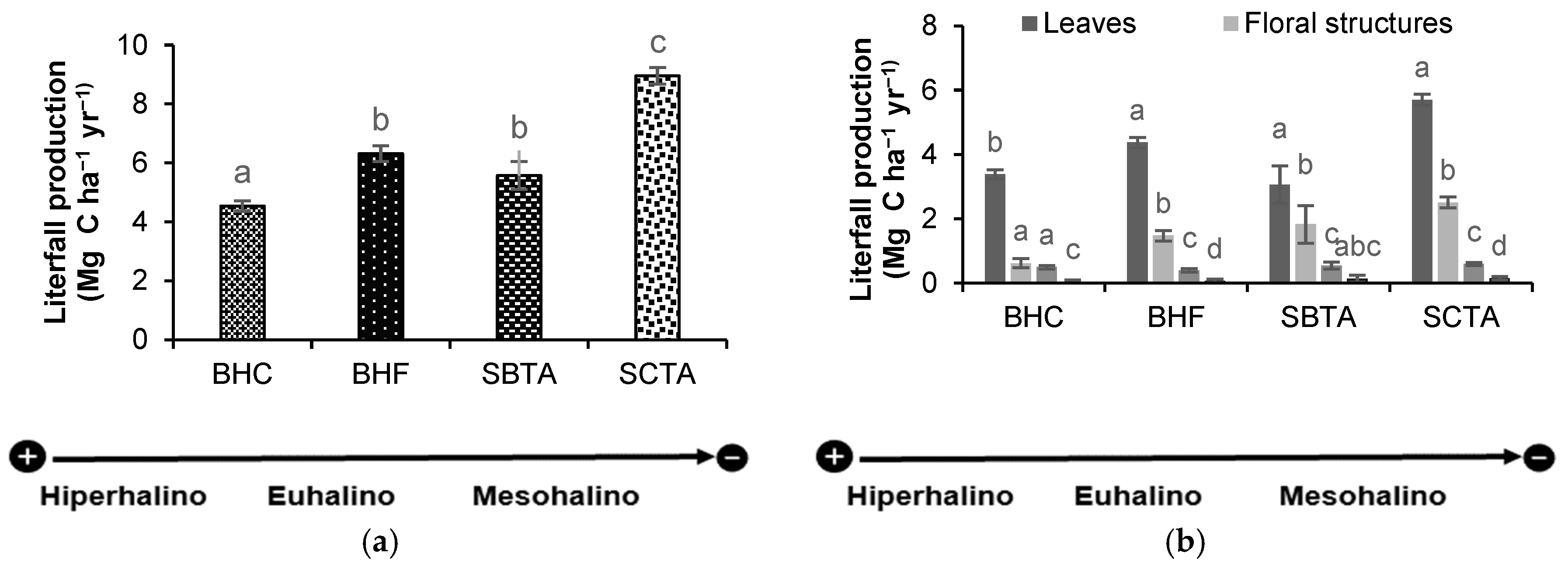
Figure 2.
Litterfall production in Mg C ha-1 y-1 (mean ± SE) of Ag: Avicennia germinans, Lr: Laguncularia racemosa and Rm: Rhizophora mangle from the mangrove forests of San Andres Island, Colombia (BHC: Bahía Hooker Cuenca; BHF: Bahía Hooker Franja; SBTA: Sound Bay Tierra Adentro; SCTA: Smith Channel Tierra Adentro). Lowercase letters denote significant differences (p<0.05) in total production between forests.
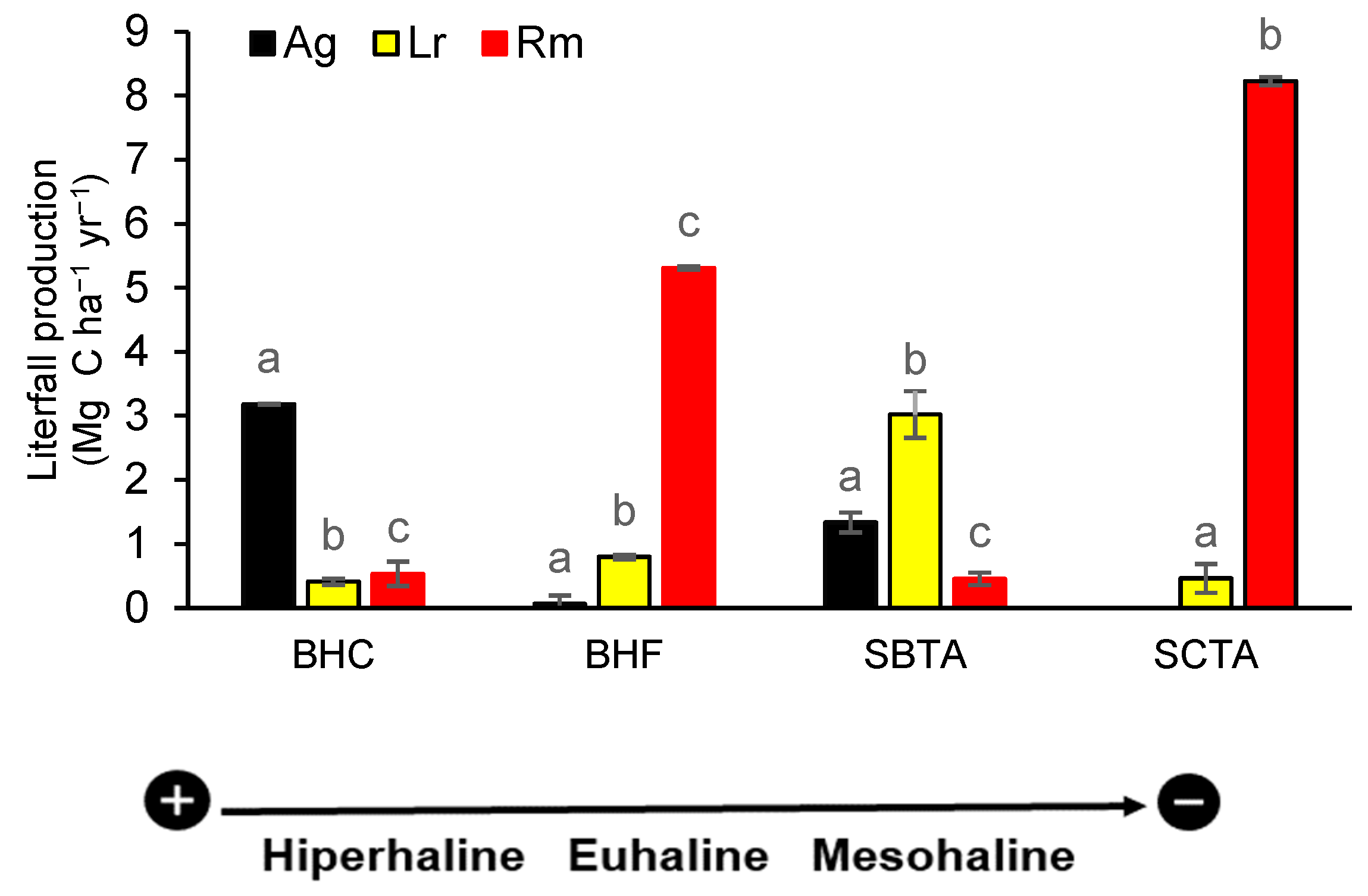
Figure 3.
Multi-annual (2012- 2019 and 2022) and multi-temporal (dry and wet season) litterfall production (Mg C ha-1y-1) (mean ± SE), of mangrove forests on San Andres Island, Colombia (BHC: Bahía Hooker Cuenca; BHF: Bahía Hooker Franja; SBTA: Sound Bay Tierra adentro; SCTA: Smith Channel Tierra adentro).
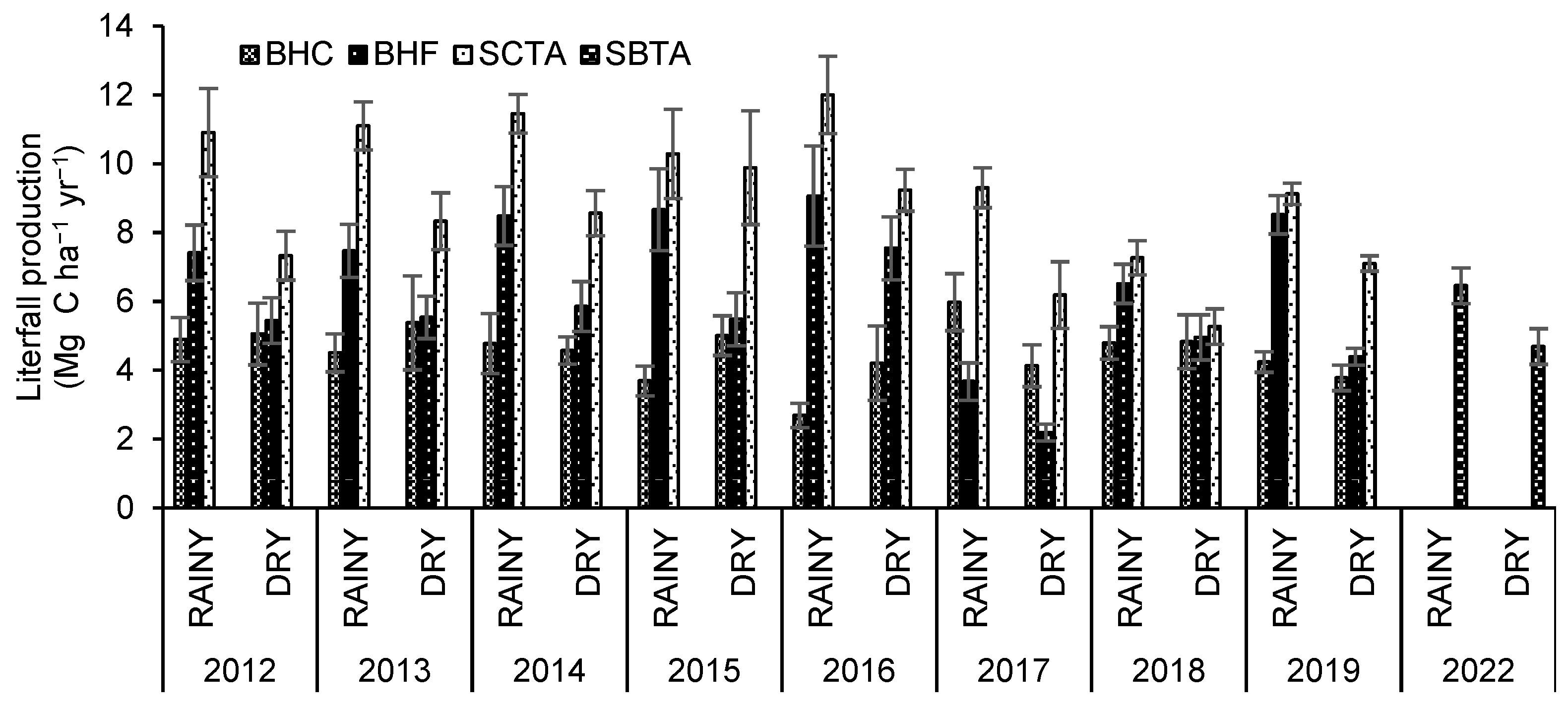
Figure 4.
Climatic variables presented during the years 2012 to 2019 and 2022 on the island of San Andres, Colombia: (a). Average cumulative precipitation (mm). (b). Wind speed (m/s). (c). Average annual ambient temperature (°C).
Figure 4.
Climatic variables presented during the years 2012 to 2019 and 2022 on the island of San Andres, Colombia: (a). Average cumulative precipitation (mm). (b). Wind speed (m/s). (c). Average annual ambient temperature (°C).
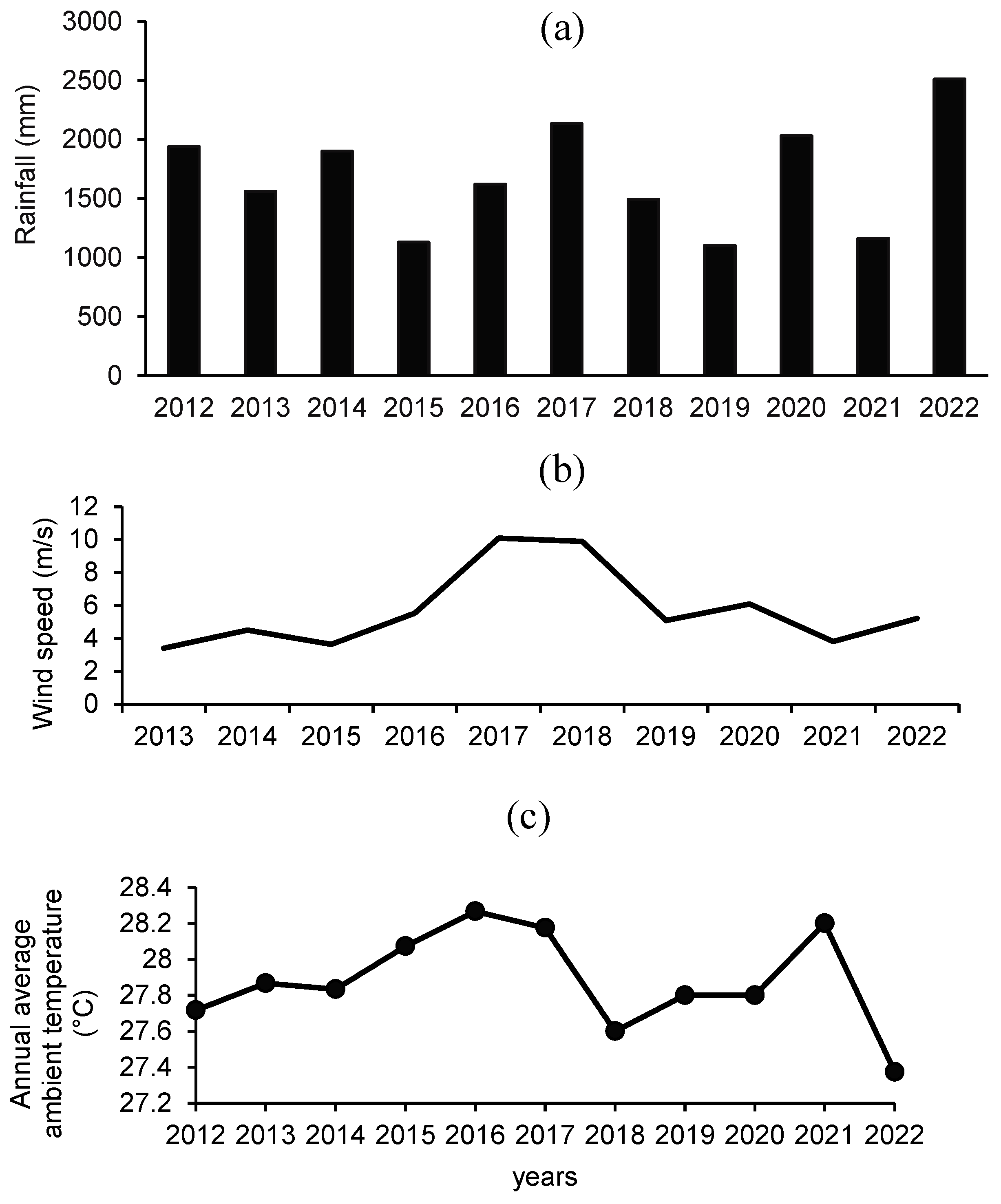
Figure 5.
Linear regression lagged effect between monthly litterfall carbon content (Mg C ha-1 m-1) in the SBTA mangrove forest on San Andres Island, Colombia, and monthly salinity (PSU).
Figure 5.
Linear regression lagged effect between monthly litterfall carbon content (Mg C ha-1 m-1) in the SBTA mangrove forest on San Andres Island, Colombia, and monthly salinity (PSU).
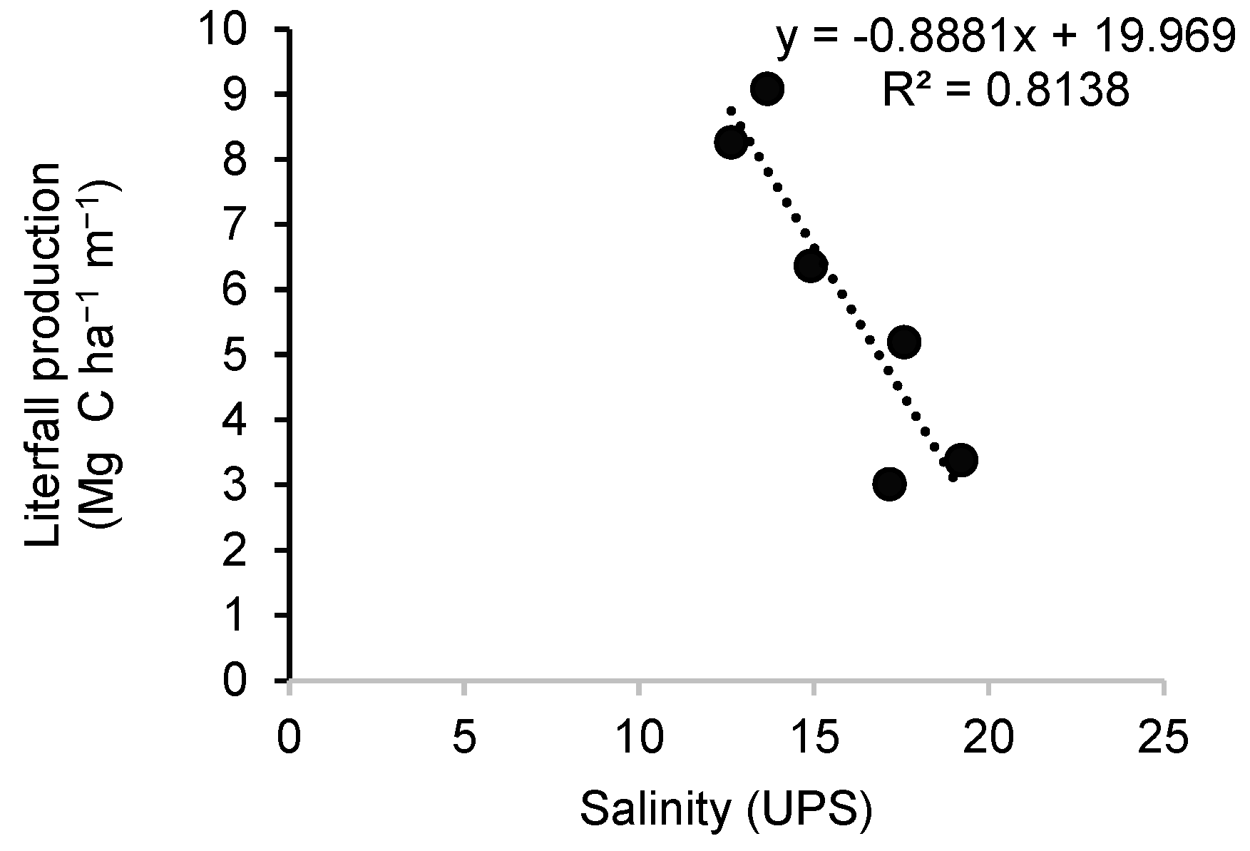
Table 1.
Structural variables characteristic of the mangrove forests of San Andres Island, Colombia (BHC: Bahía Hooker Cuenca; BHF: Bahía Hooker Franja; SBTA: Sound Bay Tierra Adentro; SCTA: Smith Channel Tierra Adentro). Diameter at breast height (DBH). Relative importance value index (IVI). Mean ± SE.
| Forest | Salinity (PSU) | Species | Density In ha-1 |
DBH (≥2.5 cm) |
Basal area (m2 ha-1) |
IVI |
|---|---|---|---|---|---|---|
| BHC | 62.4± 10.4 | Ag | 2242 ± 32.4 | 9.1 ± 0.3 | 19.8 ± 0.5 | 221 |
| Lr | 125 ± 55.9 | 10.8 ± 1.1 | 1.3 ± 0.08 | 37 | ||
| Rm | 183 ± 67.7 | 7.1 ±0.5 | 0.8 ± 0.04 | 42 | ||
| Total | 2550 ± 71.7 a | 9.1 ± 0.3 b | 21.9 ± 0.5 a | 300 | ||
| BHF | 37.5± 5.8 | Ag | 215 ± 0.5 | 8.8 ± 0.8 | 1.7 ± 0.2 | 26 |
| Lr | 920± 1.7 | 8.1 ± 0.3 | 6.3 ± 0.3 | 104 | ||
| Rm | 2520 ± 2.3 | 6.8 ± 0.1 | 10.9 ± 0.2 | 170 | ||
| Total | 3655 ± 43.7 ab | 7.3 ± 0.1b | 18.9 ± 0.4 a | 300 | ||
| SBTA | 11.5 ± 7.5 | Ag | 356 ± 0.5 | 14.8 ± 1.1 | 9.8 ± 1.2 | 133 |
| Lr | 188 ± 0.8 | 27.6 ± 2 | 13.2 ± 2 | 99 | ||
| Rm | 194 ± 1.1 | 13.04 ± 1.5 | 4.2 ± 0.8 | 68 | ||
| Total | 738 ± 8.8 b | 18.5 ± 0.73 b | 27.3 ± 0.4 b | 300 | ||
| SCTA | 9.6± 6.3 | Lr | 75±13 | 34.1 ± 1.4 | 9.6 ± 2.6 | 61 |
| Rm | 313 ± 24 | 28.5 ± 0.7 | 28.2 ± 0.1 | 182 | ||
| Other spp. | 16± 9 | 7.2 ± 0.4 | 58 | |||
| Total | 404± 26 ab | 23.3 ± 8.2b | 37.8 ± 2.5 b | 300 | ||
| Df | 3 | 3 | 3 | |||
| P | 0.01073 | 0.006131 | 0.05688 | |||
| X2 | 11.192 | 12.4 | 7.5267 | |||
* Mangrove species: Ag: Avicennia germinans, Lr: Laguncularia racemosa and Rm: Rhizophora mangle.
Table 2.
Total root production (Mg C ha-1y-1) (mean ± SE) by size < 2 mm, 2 - 5 mm and > 5 mm in mangrove forests of San Andres Island, Colombia (BHC: Bahía Hooker Cuenca; BHF: Bahía Hooker Franja; SBTA: Sound Bay Tierra Adentro; SCTA: Smith Channel Tierra Adentro).
Table 2.
Total root production (Mg C ha-1y-1) (mean ± SE) by size < 2 mm, 2 - 5 mm and > 5 mm in mangrove forests of San Andres Island, Colombia (BHC: Bahía Hooker Cuenca; BHF: Bahía Hooker Franja; SBTA: Sound Bay Tierra Adentro; SCTA: Smith Channel Tierra Adentro).
| Size of roots | ||||
|---|---|---|---|---|
| Forest | < 2 mm Mg C ha-1y-1 |
2 - 5 mm Mg C ha-1y-1 |
> 5 mm Mg C ha-1y-1 |
Total Mg C ha-1y-1 |
| BHC | 0.08 ±0.06 | 0.09 ± 0.07 | 0.07 ± 0.10 | 0.24 ± 0.20 ab |
| BHF | 0.48 ± 0.30 | 0.28 ± 0.10 | 0.54 ± 0.34 | 1.30 ± 0.5 a |
| SBTA | 0.41 ± 0.08 | 0.24 ± 0.07 | 0.54 ± 0.36 | 1.19 ± 0.46 ab |
| SCTA | 0.16 ± 0.03 | 0.10 ± 0.02 | 0.16 ± 0.06 | 0.41± 0.08 a |
| P | 0.0007887 | 0.0002478 | 0.02384 | 0.005174 |
| Df | 3 | 3 | 3 | 3 |
| X2 | 16.77 | 19.21 | 9.45 | 12.76 |
Table 3.
Mean values of interstitial salinity in the mangrove forests of the BHC, BHF SBTA and SCTA on San Andres Island, Colombia (BHC: Bahía Hooker Cuenca; BHF: Bahía Hooker Franja; SBTA: Sound Bay Tierra Adentro; SCTA: Smith Channel Tierra Adentro), in the dry and rainy seasons. Lower case letters were used to indicate significant differences.
| Forest | PSU anual | PSU by period | |
|---|---|---|---|
| Rainy | Dry | ||
| BHC | 62.3 ±10.5 a | 60.7± 0.9 a | 62.5± 1.0 a |
| BHF | 37.4 ± 5.7 b | 36.6± 0.4 b | 39.0± 0.3 b |
| SBTA | 11.5± 7.4 c | 9.4± 0.6 c | 17.0± 0.8d |
| SCTA | 9.6± 6.2 d | 9.5± 0.4 c | 9.8 ± 0.5 c |
Table 4.
Results of the correlations between annual litterfall production and average wind speed (Ws average), annual accumulated precipitation (P) and average temperature (T). * indicates significant correlations (P< 0.05).
Table 4.
Results of the correlations between annual litterfall production and average wind speed (Ws average), annual accumulated precipitation (P) and average temperature (T). * indicates significant correlations (P< 0.05).
| Production Forest (Mg C Ha-1y-1) |
Ws Prom m/s |
P Mm |
T °C |
|||
|---|---|---|---|---|---|---|
| R | P | R | P | r | p | |
| BHC | -0.73 | 0.0394* | 0.16 | 0.6963 | 0.10 | 0.8186 |
| BHF | 0.46 | 0.2508 | 0.12 | 0.7820 | -0.36 | 0.3794 |
| SCTA | 0.38 | 0.3489 | 0.43 | 0.2916 | -0.23 | 0.5800 |
Table 5.
Results of correlations between monthly litterfall production and monthly average wind speed (Ws Prom), monthly accumulated precipitation (P) and monthly average temperature (T). * indicates a significant correlation at P< 0.05.
Table 5.
Results of correlations between monthly litterfall production and monthly average wind speed (Ws Prom), monthly accumulated precipitation (P) and monthly average temperature (T). * indicates a significant correlation at P< 0.05.
| Production Forest (Mg C Ha-1m-1) |
Salinity PSU |
Ws Prom m/s |
P Mm |
T °C |
||||
|---|---|---|---|---|---|---|---|---|
| R | P | R | P | R | P | r | P | |
| SBTA | -0.21 | 0.5024 | -0.21 | 0.5070 | 0.45 | 0.1464 | 0.22 | 0.4820 |
Disclaimer/Publisher’s Note: The statements, opinions and data contained in all publications are solely those of the individual author(s) and contributor(s) and not of MDPI and/or the editor(s). MDPI and/or the editor(s) disclaim responsibility for any injury to people or property resulting from any ideas, methods, instructions or products referred to in the content. |
© 2025 by the authors. Licensee MDPI, Basel, Switzerland. This article is an open access article distributed under the terms and conditions of the Creative Commons Attribution (CC BY) license (http://creativecommons.org/licenses/by/4.0/).
Copyright: This open access article is published under a Creative Commons CC BY 4.0 license, which permit the free download, distribution, and reuse, provided that the author and preprint are cited in any reuse.


