Submitted:
23 January 2025
Posted:
24 January 2025
You are already at the latest version
Abstract
The inability of borrowers to repay loans poses a significant challenge to the sustainability of the peer-to-peer (P2P) lending sector. This study leverages predictive modelling techniques to analyze historical applicant data from Lending Club, focusing on reducing late payments through the proprietary Sriya Expert Index (SXI) AI-ML algorithm. SXI serves as a super feature, synthesizing the outputs of 5-10 machine learning algorithms into a simplified score/index, enabling accurate prediction of late payments. The model dynamically adjusts algorithmic weights to optimize precision, considering critical features such as credit history, income, and repayment behavior. In comparison to traditional machine learning models, the Sriya Expert Index (SXI) algorithm significantly outperforms established approaches in predicting late payments. Models such as Random Forest and XGBoost achieved accuracies of 78.80% and 84.52%, respectively, while the Mixture of Experts (MOE) neural network reached 92.10%. The Support Vector Machine (SVM) with a linear kernel delivered an AUC of 0.935, slightly higher than the 0.92 AUC of XGBoost. However, SXI surpasses all these models with a near flawless accuracy of 99.80% and an AUC score of 0.998. This demonstrates the model's superiority in identifying late payment risks and its potential to guide effective intervention strategies. One of the standout features of SXI enabled AI-ML is to improve business outcomes with actionable insights. The study outlines a phased methodology for reducing late payments (desired business outcome), achieving an initial 20% reduction and further improvements to 50% and 80% in the mid-term and long-term, respectively. These findings highlight the transformative potential of SXI in enhancing risk management in P2P lending, offering a scalable, data-driven solution to improve the financial health of the sector.
Keywords:
SXI
; P2P lending platform
; Lending Club
; reducing late payments
; predictive model
1. Introduction
Traditional financial institutions have high thresholds, low returns, and long investment cycles, driving investors to seek more flexible, higher-yield, and lower-amount investment options. However, limitations in the personal credit information system and slow credit infrastructure development prevent some deserving individuals from accessing funds, leading to the rise of streamlined platforms like P2P lending. P2P platforms act as intermediaries, connecting borrowers and lenders online. They offer convenient and accessible lending and money transfer services. Additionally, deep learning techniques provide valuable insights for interpreting various forms of data, potentially enhancing the functionality of P2P platforms (Liu D., 2015). The demand from both investors and borrowers has fueled the growth of P2P lending platforms significantly, contributing to their rapid expansion. These platforms have become integral to the financial market in my country, fulfilling crucial roles in meeting investment and financing demands while fostering market diversity. However, despite their importance, P2P platforms suffer from deficiencies in financial management and risk control capabilities, leading to a considerable number of defaulted loans (Ge R., 2017).
The largest P2P lending platform in the United States, known as “Lending Club” operates as an online platform that bypasses traditional financial institutions, linking numerous investors with potential borrowers to facilitate capital investment and credit borrowing. Borrowers can submit loan requests detailing the purpose of the loan along with their personal financial details. Investors have the flexibility to select the amount of capital they wish to invest and can also choose the specific borrower.
In this market, individuals with poor credit history, who might otherwise struggle to obtain credit from traditional financial sources or face high-interest rates, have the chance to access credit at lower rates. Conversely, investors can potentially earn higher returns on their capital compared to traditional bank savings accounts. Nevertheless, there exists a significant risk of borrowers defaulting on their loans, resulting in non-repayment of both the principal amount and interest (Magee 2011).
ML principles are applied to assess default risk, or the likelihood of a borrower failing to repay, through techniques like Neural Networks (NN) with backpropagation, as demonstrated by Zhang (2014). This NN achieved an accuracy rate of 78.6%. Freedman and Jin (2008) found a positive correlation between borrowers' credit ratings and loan success rates. Fu (2017) conducted experiments merging tree methods like Random Forest (RF) with Neural Networks (NN). Milad (2005) investigated factors such as loan grade (a Lending Club-assigned score for borrowers) and Fair Isaac Corporation scores (FICO) as predictors of default risk. Milad employed various learning algorithms, including a cost-based RF, which attained the top accuracy score of 78.8%. These studies all approached the task of assessing default risk as a classification problem. Methods such as BPNN create a loan default prediction model, enabling effective assessment of default risk probability and lowering risk management costs by achieving an AUC Score of 0.79 and a default loan prediction accuracy of 84.05% (Li.B, 2022).
However, upon closer examination, it was noted that the classification variable, often labeled as loan_status, exhibited an imbalance in instances. Specifically, instances where borrowers did not default were substantially more prevalent than instances of default. This class imbalance poses challenges for classification models, as they may become biased toward the majority class, potentially leading to overfitting issues, as demonstrated by Chawla (2001).
Using Data mining techniques particularly on Support Vector Machine (SVM), are employed to identify distinctive patterns among customers in Indonesia with defaulted and non-defaulted credit. Analyzing 100 borrower records spanning from March 2017 to January 2019, including social media features, revealed SVM Linear as the optimal model, outperforming SVM RBF and SVM Poly. Specifically, SVM Linear exhibited an AUC of 0.935, while SVM RBF and SVM Poly achieved only 0.755 and 0.42 respectively (Saputra, 2021).
In a study conducted by Feller using Lending Club loan data, the aim was to assess the explanatory capability of hard data and its sufficiency in understandable user behavior on the platform during their initial iteration. Two multiple logistic regression analyses were undertaken to evaluate the influence of hard data variables on funding receipt and loan charge-off likelihood within Lending Club. The hard data related to loan repayment accounts for 12.2% of the variance among borrowers whose loans have been charged off. Analysis of borrower data indicates that a lower credit grade, lower FICO range, and higher monthly income are associated with a decreased likelihood of defaulting on investment, while higher interest rates are negatively correlated with default probability (Feller, 2017).
Another study conducted by Miller Janny integrates profit information into the entire modeling process, including XGBoost learning function, model tuning, and decision-making stages. The results demonstrated that profit-based models could yield higher financial returns while reshaping the role of input variables, favoring factors like low indebtedness and small loan amounts for low-risk, profitable lending. However, the models showed low acceptance rates, reflecting the complexity and risk of the small business segment (Miller-Janny Ariza-Garzón, 2024). In a study exploring credit risk modelling, a mixture-of-experts (MOE) neural network framework was utilized to predict default probabilities on peer-to-peer lending platforms, achieving a high accuracy of 92.10% (Makokha, 2024). By combining supervised and unsupervised machine learning techniques, hybrid models demonstrated superior performance in handling complex, nonlinear relationships compared to traditional supervised models. (Machado, 2022).
Previous studies predominantly employed machine learning techniques to address the challenge of predicting late payments in peer-to-peer (P2P) lending platforms, focusing primarily on identifying high-risk borrowers. However, these approaches often lacked interpretability regarding the influence of key borrower characteristics and financial behaviors on late payment predictions, failed to propose effective strategies for reducing late payments over short-, mid-, and long-term periods, and relied on models that required extensive prior training. Additionally, there was limited integration of advanced scoring systems, which could leverage diverse borrower data, such as credit history, income stability, and repayment trends, to more accurately assess late payment risks across various lending scenarios. By incorporating a comprehensive scoring system, the potential for more precise and actionable risk analysis is greatly enhanced, offering lenders a holistic understanding of borrower repayment behavior.
To address these gaps, this study focuses on: (i) evaluating the performance of the SXI algorithm as a multivariate scoring system to predict late payment risk as a binary classification problem, (ii) enhancing the SXI scoring methodology using a Proprietary Deep Neural Network algorithm and correlating it with late payment rates over a defined period, and (iii) employing a targeted decision tree framework to interpret the most effective pathways leading to both high- and low-risk borrowers, thereby offering evidence-based recommendations for reducing late payment incidences and improving the financial stability of P2P lending platforms.
2Materials and Methods
2.1. Data Description
The source of the data for this paper on predicting and reducing the impact of late loan payments using Lending Club’s historical loan applicant information likely comes from Lending Club’s internal database or archives dated from 2007 to 2020 Q3. Lending Club is a US peer-to-peer lending company, headquartered in San Francisco, California. It was the first peer-to-peer lender to register its offerings as securities with the Securities and Exchange Commission (SEC), and to offer loan trading on a secondary market.
The data given contains information about past loan applicants and whether they have late or not yet defaulted on their payments. The aim is to identify patterns which indicate if a person is likely to make late payments, which may be used for takin actions such as denying the loan, reducing the amount of loan, lending (high risky applicants) at a higher interest rate, etc.
The initial dataset consists of 2,260,668 rows and 151 features and through further data cleaning 58 features had null values exceeding 35% of the total entries. Given the significant proportion of missing data in these features was dropped from the dataset which resulted in a reduction in the number of features to 93 which will be used for further data analysis.

Table 1.
Dataset Feature Description.
| Features | Feature Description |
|---|---|
| id | A unique LC assigned ID for the loan listing. |
| acc_now_delinq | The number of accounts on which the borrower is now delinquent. |
| acc_open_past_24mths | Number of trades opened in past 24 months. |
| addr_state | The state provided by the borrower in the loan application. |
| annual_inc | The self-reported annual income provided by the borrower during registration. |
| application_type | Indicates whether the loan is an individual application or a joint application with two co-borrowers. |
| avg_cur_bal | Average current balance of all accounts. |
| bc_open_to_buy | Total open to buy on revolving bankcards. |
| bc_util | Ratio of total current balance to high credit/credit limit for all bankcard accounts. |
| chargeoff_within_12_mths | Number of charge-offs within 12 months. |
| collections_12_mths_ex_med | Number of collections in 12 months excluding medical collections. |
| delinq_2yrs | The number of 30+ days past-due incidences of delinquency in the borrower's credit file for the past. |
| delinq_amnt | The past-due amount owed for the accounts on which the borrower is now delinquent. |
| dti | A ratio calculated using the borrower’s total monthly debt payments on the total debt obligations. |
| emp_length | Employment length in years. Possible values are between 0 and 10 where 0 means less than one year. |
| emp_title | The job title supplied by the Borrower when applying for the loan. |
| fico_range_high | The upper boundary ranges the borrower’s FICO at loan origination belongs to. |
| fico_range_low | The lower boundary ranges the borrower’s FICO at loan origination belongs to. |
| funded_amnt | The total amount committed to that loan at that point in time. |
| funded_amnt_inv | The total amount committed by investors for that loan at that point in time. |
| grade | LC assigned loan grade |
| home_ownership | The home ownership status provided by the borrower during registration. |
| initial_list_status | The initial listing status of the loan. Possible values are – W, F |
| inq_last_6mths | The number of inquiries in past 6 months (excluding auto and mortgage inquiries) |
| installment | The monthly payment owed by the borrower if the loan originates. |
| int_rate | Interest Rate on the loan. |
| last_fico_range_high | The upper boundary ranges the borrower’s last FICO pulled belongs to. |
| last_fico_range_low | The lower boundary ranges the borrower’s last FICO pulled belongs to. |
| last_pymnt_amnt | Last total payment amount received. |
| loan_amnt | The listed amount of the loan applied for by the borrower. |
| mo_sin_old_il_acct | Months since oldest bank installment account opened. |
| mo_sin_old_rev_tl_op | Months since oldest revolving account opened. |
| mo_sin_rcnt_rev_tl_op | Months since most recent revolving account opened. |
| mo_sin_rcnt_tl | Months since most recent account opened. |
| mort_acc | Number of mortgage accounts. |
| mths_since_recent_bc | Months since most recent bankcard account opened. |
| mths_since_recent_inq | Months since most recent inquiry. |
| num_accts_ever_120_pd | Number of accounts ever 120 or more days past due. |
| num_actv_bc_tl | Number of currently active bankcard accounts. |
| num_actv_rev_tl | Number of currently active revolving trades. |
| num_bc_sats | Number of satisfactory bankcard accounts. |
| num_bc_tl | Number of bankcard accounts. |
| num_il_tl | Number of installment accounts. |
| num_op_rev_tl | Number of open revolving accounts. |
| num_rev_accts | Number of revolving accounts. |
| num_rev_tl_bal_gt_0 | Number of revolving trades with balance >0. |
| num_sats | Number of satisfactory accounts. |
| num_tl_120dpd_2m | Number of accounts currently 120 days past due (updated in past 2 months). |
| num_tl_30dpd | Number of accounts currently 30 days past due (updated in past 2 months). |
| num_tl_90g_dpd_24m | Number of accounts 90 or more days past due in last 24 months. |
| num_tl_op_past_12m | Number of accounts opened in past 12 months. |
| open_acc | The number of open credit lines in the borrower's credit file. |
| out_prncp | Remaining outstanding principal for total amount funded |
| out_prncp_inv | Remaining outstanding principal for portion of total amount funded by investors. |
| pct_tl_nvr_dlq | Percent of trades never delinquent. |
| percent_bc_gt_75 | Percentage of all bankcard accounts > 75% of limit. |
| policy_code | publicly available policy_code=1 new products not publicly available policy_code=2. |
| pub_rec | Number of derogatory public records. |
| pub_rec_bankruptcies | Number of public record bankruptcies. |
| purpose | A category provided by the borrower for the loan request. |
| pymnt_plan | Indicates if a payment plan has been put in place for the loan. |
| revol_bal | Total credit revolving balance. |
| revol_util | Revolving line utilization rate. |
| sub_grade | LC assigned loan subgrade. |
| tax_liens | Number of tax liens. |
| term | The number of payments on the loan. Values are in months and can be either 36 or 60. |
| tot_coll_amt | Total collection amounts ever owed. |
| tot_cur_bal | Total current balance of all accounts. |
| tot_hi_cred_lim | Total high credit limit. |
| total_acc | The total number of credit lines currently in the borrower's credit file. |
| total_bal_ex_mort | Total credit balance excluding mortgage. |
| total_bc_limit | Total bankcard high credit/credit limit. |
| total_il_high_credit_limit | Total installment high credit/credit limit. |
| total_pymnt | Payments received to date for total amount funded. |
| total_pymnt_inv | Payments received to date for portion of total amount funded by investors. |
| total_rec_int | Interest received to date. |
| total_rec_late_fee | Late fees received to date. |
| total_rec_prncp | Principal received to date. |
| total_rev_hi_lim | Total revolving high credit/credit limit. |
| verification_status | Indicates if income was verified by LC, not verified, or if the income source was verified. |
| hardship_flag | Flags whether or not the borrower is on a hardship plan |
| disbursement_method | The method by which the borrower receives their loan. Possible values are: CASH, DIRECT_PAY. |
| debt_settlement_flag | Flags whether or not the borrower, who has charged-off, is working with a debt-settlement company. |
| loan_status | Status of the loan (Current/Ongoing or Late Payments). |
The target variable for this analysis is the Loan Status (Figure 1), which has two categories: "Current" and "Late Payments" from the reformatted data. The "Current" category represents applicants who are in the process of paying their loan installments, meaning the loan tenure has not yet been completed. The "Late-Payments" category represents applicants who have paid their installments after the due date. To ensure a balanced dataset for model building, a random sample of 26,000 records was taken from the "Current" category and combined with the 25,816 records from the "Late Payments" category (Late (31 – 120 days) and Late (16 – 30 days)), resulting in a final dataset of 51,816 rows.
The dataset contains a mix of categorical and numerical features. There are 16 categorical features, and 69 numerical features. It's worth noting that 2 features, both categorical and numerical, had only 1 unique value across the entire dataset, which may indicate limited variability in those features. In addition to the categorical and numerical features, the dataset also includes 8 features that are related to dates, IDs, zip codes, and other non-predictive information. The categorical features are one hot encoded thus increasing the number of features from 82 to 171 features. The final dataset used for model building will consist of 51,816 rows and 171 features, after excluding 35% of missing values and the non-predictive features.
2.2. Descriptive Statistics
2.2.1. Missing Values
The dataset reveals significant missing values in the top 10 features (Figure 2), with open_acc_6m having the highest at 85.36%, followed by open_il_12m (84.11%). Key secondary applicant features like FICO range (high) (79%) and FICO range (low) (78.01%) also exhibit substantial missingness. Other notable features, including open_il_24m (78.12%), open_act_il (73.97%), and sec_app_inq_last_6mths (70.25%), show similar trends. Features such as sec_app_open_acc and sec_app_revol_util (both 68.04%) and sec_app_open_act_il (66.66%) indicate critical gaps in credit-related attributes. Overall, 58 features with missing values exceeding 35% of total entries were dropped from the dataset. This reduction resulted in 93 features being retained for further data analysis, ensuring better data quality and improved modeling potential.
2.2.2. Descriptive Analysis of Numerical Features
Table 2.
Summary Statistics of Numerical Features.
| Features | Mean | Std. Dev | Min Value | 25 %ile | 50 %ile | 75 %ile | Max Value |
|---|---|---|---|---|---|---|---|
| loan_amnt | 16472 | 9776 | 1000 | 9600 | 15000 | 23450 | 40000 |
| funded_amnt | 16472 | 9776 | 1000 | 9600 | 15000 | 23450 | 40000 |
| funded_amnt_inv | 16468 | 9774 | 750 | 9600 | 15000 | 23431 | 40000 |
| int_rate | 14 | 5 | 5 | 10 | 14 | 17 | 31 |
| installment | 479 | 283 | 8 | 271 | 405 | 640 | 1715 |
| annual_inc | 78547 | 81756 | 0 | 46000 | 65000 | 94000 | 9573072 |
| dti | 20 | 18 | 0 | 12 | 19 | 26 | 999 |
| delinq_2yrs | 0 | 1 | 0 | 0 | 0 | 0 | 36 |
| fico_range_low | 698 | 32 | 660 | 670 | 690 | 715 | 845 |
| fico_range_high | 702 | 32 | 664 | 674 | 694 | 719 | 850 |
| inq_last_6mths | 1 | 1 | 0 | 0 | 0 | 1 | 6 |
| open_acc | 12 | 6 | 0 | 8 | 11 | 15 | 62 |
| pub_rec | 0 | 1 | 0 | 0 | 0 | 0 | 45 |
| revol_bal | 16182 | 22897 | 0 | 5595 | 11061 | 19773 | 1392002 |
| revol_util | 49 | 25 | 0 | 30 | 48 | 68 | 143 |
| total_acc | 23 | 12 | 2 | 14 | 21 | 29 | 148 |
| out_prncp | 10837 | 8385 | 0 | 4276 | 8749 | 15418 | 40000 |
| out_prncp_inv | 10835 | 8384 | 0 | 4275 | 8747 | 15412 | 40000 |
| total_pymnt | 8533 | 7694 | 0 | 2971 | 6102 | 11682 | 60511 |
| total_pymnt_inv | 8530 | 7691 | 0 | 2971 | 6101 | 11679 | 60424 |
| total_rec_prncp | 5635 | 5344 | 0 | 1867 | 3906 | 7609 | 40000 |
| total_rec_int | 2891 | 3089 | 0 | 822 | 1788 | 3882 | 27394 |
| total_rec_late_fee | 8 | 34 | 0 | 0 | 0 | 0 | 1484 |
| last_pymnt_amnt | 512 | 739 | 0 | 264 | 402 | 646 | 38341 |
| last_fico_range_high | 659 | 75 | 0 | 599 | 669 | 714 | 850 |
| last_fico_range_low | 647 | 109 | 0 | 595 | 665 | 710 | 845 |
| collections_12_mths_ex_med | 0 | 0 | 0 | 0 | 0 | 0 | 6 |
| policy_code | 1 | 0 | 1 | 1 | 1 | 1 | 1 |
| acc_now_delinq | 0 | 0 | 0 | 0 | 0 | 0 | 2 |
| tot_coll_amt | 220 | 1712 | 0 | 0 | 0 | 0 | 197765 |
| tot_cur_bal | 137087 | 160456 | 0 | 27349 | 68989 | 204094 | 4170862 |
| total_rev_hi_lim | 34290 | 34783 | 0 | 14500 | 25600 | 43100 | 1656900 |
| acc_open_past_24mths | 5 | 3 | 0 | 2 | 4 | 6 | 43 |
| avg_cur_bal | 12847 | 15910 | 0 | 2940 | 6581 | 17599 | 370743 |
| bc_open_to_buy | 11577 | 16591 | 0 | 2021 | 5798 | 14476 | 284588 |
| bc_util | 56 | 29 | 0 | 33 | 57 | 81 | 216 |
| chargeoff_within_12_mths | 0 | 0 | 0 | 0 | 0 | 0 | 3 |
| delinq_amnt | 12 | 689 | 0 | 0 | 0 | 0 | 112524 |
| mo_sin_old_il_acct | 124 | 55 | 1 | 91 | 129 | 153 | 686 |
| mo_sin_old_rev_tl_op | 176 | 101 | 2 | 109 | 157 | 227 | 800 |
| mo_sin_rcnt_rev_tl_op | 14 | 18 | 0 | 4 | 8 | 17 | 368 |
| mo_sin_rcnt_tl | 8 | 9 | 0 | 3 | 6 | 11 | 368 |
| mort_acc | 1 | 2 | 0 | 0 | 1 | 2 | 23 |
| mths_since_recent_bc | 24 | 32 | 0 | 6 | 14 | 28 | 487 |
| mths_since_recent_inq | 7 | 6 | 0 | 2 | 5 | 10 | 24 |
| num_accts_ever_120_pd | 1 | 1 | 0 | 0 | 0 | 0 | 34 |
| num_actv_bc_tl | 4 | 2 | 0 | 2 | 3 | 5 | 25 |
| num_actv_rev_tl | 6 | 4 | 0 | 3 | 5 | 7 | 44 |
| num_bc_sats | 5 | 3 | 0 | 3 | 4 | 6 | 37 |
| num_bc_tl | 7 | 5 | 0 | 4 | 6 | 9 | 49 |
| num_il_tl | 8 | 7 | 0 | 3 | 6 | 11 | 99 |
| num_op_rev_tl | 8 | 5 | 0 | 5 | 7 | 11 | 60 |
| num_rev_accts | 13 | 8 | 2 | 8 | 12 | 17 | 116 |
| num_rev_tl_bal_gt_0 | 6 | 3 | 0 | 3 | 5 | 7 | 41 |
| num_sats | 12 | 6 | 0 | 7 | 11 | 15 | 62 |
| num_tl_120dpd_2m | 0 | 0 | 0 | 0 | 0 | 0 | 1 |
| num_tl_30dpd | 0 | 0 | 0 | 0 | 0 | 0 | 2 |
| num_tl_90g_dpd_24m | 0 | 0 | 0 | 0 | 0 | 0 | 36 |
| num_tl_op_past_12m | 2 | 2 | 0 | 1 | 2 | 3 | 18 |
| pct_tl_nvr_dlq | 94 | 10 | 0 | 91 | 98 | 100 | 100 |
| percent_bc_gt_75 | 40 | 36 | 0 | 0 | 33 | 67 | 100 |
| pub_rec_bankruptcies | 0 | 0 | 0 | 0 | 0 | 0 | 7 |
| tax_liens | 0 | 0 | 0 | 0 | 0 | 0 | 45 |
| tot_hi_cred_lim | 172769 | 179167 | 0 | 49018 | 104864 | 249270 | 4562297 |
| total_bal_ex_mort | 52443 | 52269 | 0 | 20842 | 38610 | 66228 | 1392002 |
| total_bc_limit | 23092 | 23117 | 0 | 8300 | 16400 | 30000 | 711400 |
| total_il_high_credit_limit | 45790 | 46841 | 0 | 15443 | 34084 | 61867 | 976075 |
2.2.3. Loan Amount vs Interest Rate vs Loan Status
The descriptive statistics for loan amounts indicate a noticeable difference in the distribution between Current and Late payments. On average, borrowers with late payments tend to take slightly higher loan amounts ($17,021.50) compared to those who are current ($15,926.56). Additionally, (Figure 3) the interquartile range (IQR) is broader for late payments ($14,000: from $10,000 to $24,000) than for current payments ($13,125: from $8,400 to $21,525), suggesting that late payments are associated with more variability in loan sizes. This difference may point to a pattern where larger loans (Figure 4) or a certain borrower profile could be contributing to increased likelihood of delinquency.
The correlation matrix (Figure 5) highlights a moderate positive relationship between interest rates and loan status (correlation = 0.27). This suggests that borrowers with higher interest rates are more likely to have late payments. However, the correlation between loan amounts and loan status (0.056) is weaker, indicating that loan size alone is not a strong predictor of payment timeliness. The weak positive correlation between interest rates and loan amounts (0.08) suggests that while larger loans may marginally attract higher rates, this is not a dominant trend. Taken together, the insights imply that interest rates might serve as a more reliable indicator of payment risk than loan amounts, pointing to potential areas for targeted risk mitigation.
2.2.4. Loan Status Distribution
The dataset used for the analysis is well-balanced across the different splits, ensuring reliable and unbiased model training, testing, and validation (Table 3). The training set comprises 36,271 records, nearly evenly divided between Late Payments (18,146 or 50.03%) and Current Payments (18,125 or 49.97%). This balance is critical for developing a model that does not favor one class over the other, particularly for binary classification problems like loan payment prediction.
Similarly, the testing set of 10,363 records maintains a near-even distribution, with 49.10% (5,088 records) classified as Late Payments and 50.90% (5,275 records) as Current Payments. The validation set also follows this trend, with 49.83% (2,582 records) representing Late Payments and 50.17% (2,600 records) as Current Payments. This consistent class distribution across all subsets (training, testing, and validation) ensures that the model's performance metrics, such as accuracy and precision, are not influenced by an imbalanced dataset, thereby enhancing the credibility of the results. Overall, the dataset's balance supports robust statistical analysis and reliable model evaluation.
2.3. Method
2.3.1. SXI Score Calculation
SXI is a dynamic score/index obtained from a proprietary formula consisting of weights from 5-10 ML algorithms (S. Kilambi, 2024). SXI is a super feature and is a true weighted representative of all important features which converts a multi-dimensional hard-to-solve problem into a simpler 2-dimensional solution. SXI with Proprietary Deep Neural Network algorithm involves an iterative approach where it dynamically adjusts algorithm weights based on the most significant weights provided by the 5 to 10 ML algorithms. This process aims to enhance the correlation between SXI scores and business outcomes, thereby improving accuracy and delineation.
The SXI Framework (Figure 6) employs a variety of mathematical techniques ranging from arithmetic to statistical analyses and non-machine learning algorithms to process cleaned data effectively. By leveraging this diverse framework, the SXI utilizes multiple functions, including statistical measures like Standard Deviation and various types of correlations, alongside algebraic operations such as proportionality constants. Through these operations, the SXI Engine calculates a Base SXI score by bringing together various statistical analysis and algebraic computations.
The SXI Engine utilizes algebraic and statistical methods to derive weights for individual user input parameters within a user vector. These weights act as multipliers, enabling adjustments to the significance of each parameter. For example, bi-variate and multi-variate analyses may yield correlation coefficients, which are then employed as multipliers for the user vector components. This process contributes to the generation of a robust Base SXI score, serving as the foundation for subsequent steps in the SXI algorithm.
Once the Base SXI score is established, the system incorporates weights obtained from 5 to 10 machine learning algorithms. These weights collectively contribute to form the Final SXI scores, which serve as the Initial SXI or the Benchmark SXI score in the SXI algorithm. This integration of diverse mathematical functions, statistical analyses, and machine learning algorithms highlights the versatility of the SXI, providing a comprehensive approach to scoring and delineating business outcomes based on user input parameters.
Benchmark analysis of the baseline score involves extracting key metrics such as the Average SXI Score (Benchmark Score), percentage of good and bad outcomes, and the distribution of outcomes above and below the average SXI. This analysis offers insights into the performance of the SXI algorithm in distinguishing between positive and negative outcomes.
The Proprietary Deep Neural Network algorithm (Figure 7) plays a crucial role in optimizing the SXI algorithm. It adjusts weights dynamically based on the performance of the system, aiming to enhance the correlation between SXI scores and business outcomes. The Proprietary Deep Neural Network algorithm agent identifies the top features from machine learning weights and adjusts the weights accordingly. Additionally, it introduces a custom weight initialization strategy based on feature importance, aligning the weight initialization process with the significance of individual features (S. Kilambi, 2024).
The Deep Learning Architecture consists of automated hyperparameter tuning, flexibility in activation functions and optimizers, dynamic architecture based on dataset size, and structured evaluation metrics. These characteristics ensure adaptability, efficiency, and thorough evaluation of the deep neural network model.
The workflow of the Proprietary Deep Neural Network algorithm involves steps such as train-test split, in our study, we divided the dataset into 70% for training, 20% for testing, and 10% for validation. The validation set, making up 10% of the data, plays a crucial role in the design of SXI algorithm by aiding in hyperparameter tuning, overfitting detection, and appropriate model selection, ensuring that the model can generalize well to new, unseen data. Overfitting, where a model performs well on training data but poorly on real-world data, can be mitigated with the validation set. This thorough process ensures that the model is not only accurate on the training data but also reliable and generalizable. The validation dataset is thus a critical stage in the SXI workflow, confirming that the model remains highly accurate and generalizable when applied to new data. In this model, we adopted a 70-20-10 split for training, testing, and validation. This approach ensures that the model is thoroughly evaluated and fine-tuned before being tested on the 20% of data set aside for final performance assessment. The testing set, which comprises 20% of the data, is used to evaluate the model's performance and ensure its accuracy on new, unseen data.
Bayesian optimization for hyperparameter tuning, model configuration, and model training and evaluation with the best hyperparameters. Iterative weight calibration is performed to refine the SXI algorithm, where it adjusts weights, applies rewards and punishments based on performance improvements, until an optimal delineator is achieved.
In the reward and punishment mechanism, improvements in both SXI score and class delineation accuracy lead to a reward. This involves integrating the newly adjusted weights into the existing ones and recalculating SXI scores to evaluate the enhancements in delineation and accuracy. If these improvements occur without any weight adjustment, there is a positive weight adjustment, initially ranging from 0 to 100% percentage increase weights. Further iterations iteratively adjust weights until maximum accuracy is achieved. If positive adjustments fail to surpass the initial class delineation, negative weight adjustments from 0 to -100% percentage increase weights are implemented. If these adjustments yield improved delineation and accuracy, subsequent iterations continue adjusting feature weights negatively until no further improvement is possible. In cases where no improvement is observed for both positive and negative adjustments, the reinforced function penalizes by providing the next set of weights, along with additional weightage for the top 5 most important features in the hidden layers of the deep neural network.
The iterative process continues until the SXI scores cannot be further improved. The final new SXI scores are then updated to the system for further analysis and decision-making regarding business outcomes.
2.3.2. Correlation of SXI w.r.t Late Payments
In the context of business outcomes, this score can be correlated with specific classes such as "good" and "bad" within the data set. One common metric for evaluating the strength of this correlation is the coefficient of determination, often denoted as R-squared (R²).
If the SXI scores (x) are the independent variable and the target outcome (y) is the dependent variable, a polynomial regression equation can be expressed as:
where
- is the target outcome,
- is the SXI scores,
- are the coefficients representing the weights of the polynomial terms,
- is the degree of the polynomial, and
- is the error term.
The coefficient of determination, denoted as R², quantifies how well the SXI scores explain the variance in the business outcomes. By analyzing polynomial regression plots, distinct improvement phases can be identified: initial, mid-term, and long-term improvements. These phases delineate where changes in SXI scores most significantly impact business outcomes, aiding in the strategic interpretation of data trends and patterns.
2.3.3. Model Training and Evaluation
The model training process starts with hyperparameter tuning, specifically focusing on the alpha parameter. This involves adjusting the SXI score by varying the alpha value between 0.5 and 1.5 in increments of 0.1. During each iteration, the SXI score is recalculated by multiplying the current SXI score with the alpha value, enabling fine-tuning to optimize the model's performance.
where:
- is the tuning parameter, ranging from 0.5 to 1.5 in increments of 0.1,
- s the Benchmark SXI score, and
- is the new SXI score after applying the alpha adjustment.
The dataset is divided into three parts: 70% for training, 20% for testing, and 10% for validation. This strategic split ensures the model is well-trained while also providing sufficient data for testing and validation, reducing the risk of overfitting and enabling an accurate assessment of model performance. During training, the optimized SXI scores are used as a "Super Feature," playing a crucial role in enhancing the model’s predictive accuracy.
To thoroughly evaluate the model's performance, various metrics are employed. Accuracy measures the overall correctness of the model’s predictions, while precision focuses on the proportion of true positive results among all positive predictions. The confusion matrix offers a detailed breakdown of true positive, true negative, false positive, and false negative outcomes, providing deeper insights into the model’s classification abilities. Additionally, the Area Under the Curve (AUC) is utilized to assess the model's effectiveness in distinguishing between classes, serving as a robust indicator of its predictive power. Accuracy and precision are defined as:
where:
- TP is the number of true positives,
- TN is the number of true negatives,
- FP is the number of false positives, and
- FN is the number of false negatives.
The AUC for the Receiver Operating Characteristic (ROC) curve measures the classifier's ability to distinguish between positive and negative classes. It is calculated based on the True Positive Rate (TPR) and False Positive Rate (FPR), with the ROC curve plotting TPR against FPR at different threshold settings. TPR, FPR and AUC are defined as follows:
where:
- and are the true positive rates at consecutive thresholds, and
- and are the false positive rates at consecutive thresholds.
2.3.4. Actionable Insights for Reducing Late Payments
In the decision tree model, borrower and financial behavior features contributing to late payments are assigned positive weights, while those mitigating late payments are assigned negative weights. To implement strategies for reducing late payments, users specify a percentage increase for positive weighted features and a percentage decrease for negative weighted features. During the data transformation process, these adjustments are applied to each observation: positive weighted features are increased by the specified percentage, and negative weighted features are decreased, simulating an initial enhancement in the dataset to reduce late payment risks.
If the late payment risk model shows a positive correlation between SXI scores and late payment risk, the strategy for positive weighted features is:
For features that reduce late payment risk, the strategy is:
In cases where a negative correlation exists between SXI scores and late payment risk (where higher SXI scores indicate lower late payment risks), the weights are reversed. Features negatively impacting late payment risks (increasing them) are given positive weights, while features reducing late payment risks receive negative weights. Under this scenario, positive weighted features (which increase late payment risk) require a strategy involving a percentage decrease, and negative weighted features (which reduce late payment risk) call for a percentage increase.
For positive weighted features, the strategy is:
For negative weighted features the strategy is:
Once the dataset has been adjusted using these transformations, it is used to train a Random Forest model. The model learns the relationships between borrower attributes, financial behaviours, and late payment risks by analysing data through multiple decision trees. Each decision tree captures distinct aspects of the feature-risk relationship, and among these, a target decision tree path is identified. This path represents the sequence of feature splits that most accurately predicts late payment risks based on the adjusted dataset, offering a detailed understanding of the factors contributing to late payments and actionable insights into effective mitigation strategies.
3. Results and Discussions
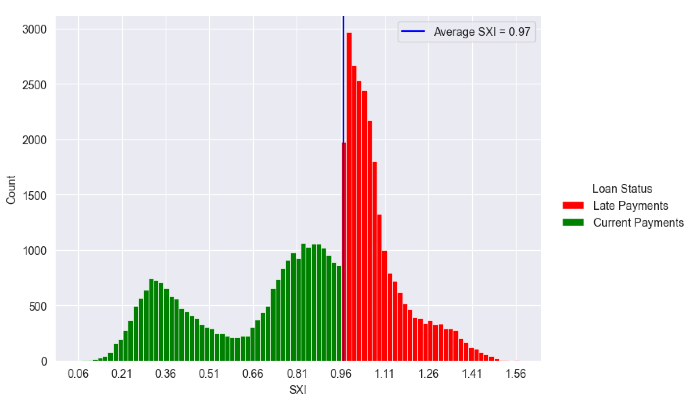
The SXI stands at 0.97, serving as the benchmark score. In terms of overall payments, 49.82% are categorized as good outcomes (current payments), while 50.18% are identified as bad outcomes (late payments). According to the initial delineation based on the benchmark, there is a slight inclination towards categorizing late payments as above SXI and current payments as below SXI.
Figure 8.
SXI Distribution. This figure shows the distribution of SXI scores, illustrating how scores differ between borrowers likely to make timely repayments and those at risk of late payments.
Figure 8.
SXI Distribution. This figure shows the distribution of SXI scores, illustrating how scores differ between borrowers likely to make timely repayments and those at risk of late payments.
The SXI algorithm demonstrated outstanding performance in classifying loan payment statuses, achieving excellent metrics across both the test and validation sets. In the test set (Figure 9), with 10,363 records, the model correctly classified 5,222 current payments and 5,037 late payments. Only 53 current payments were misclassified as late payments, and 51 late payments were misclassified as current payments. This resulted in an impressive accuracy of 99.80% and an AUC of 0.998 (Figure 11), reflecting the model's accuracy and precision in predicting loan payment outcomes.
Figure 9.
Confusion Matrix – Test Set.
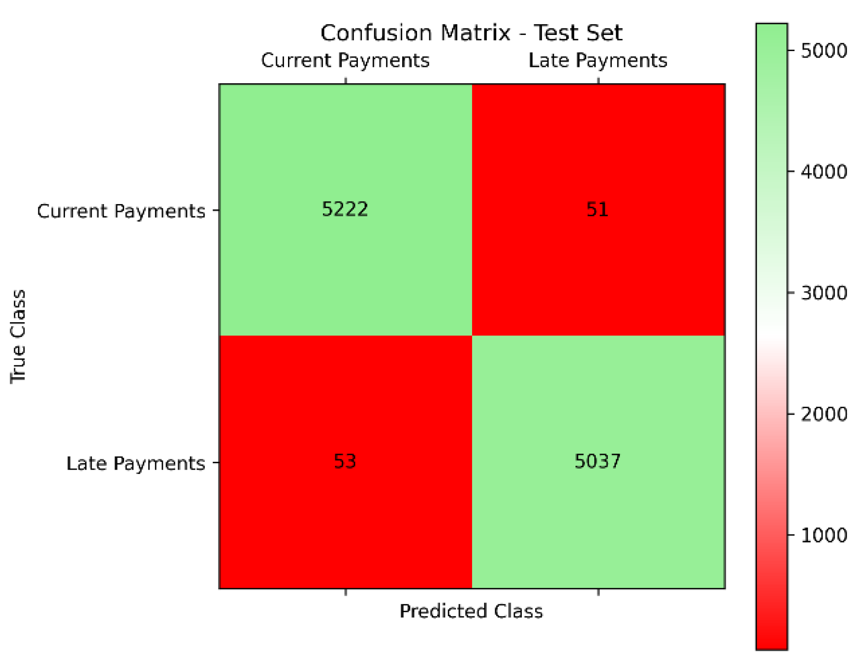
Figure 10.
Confusion Matrix – Validation Set.
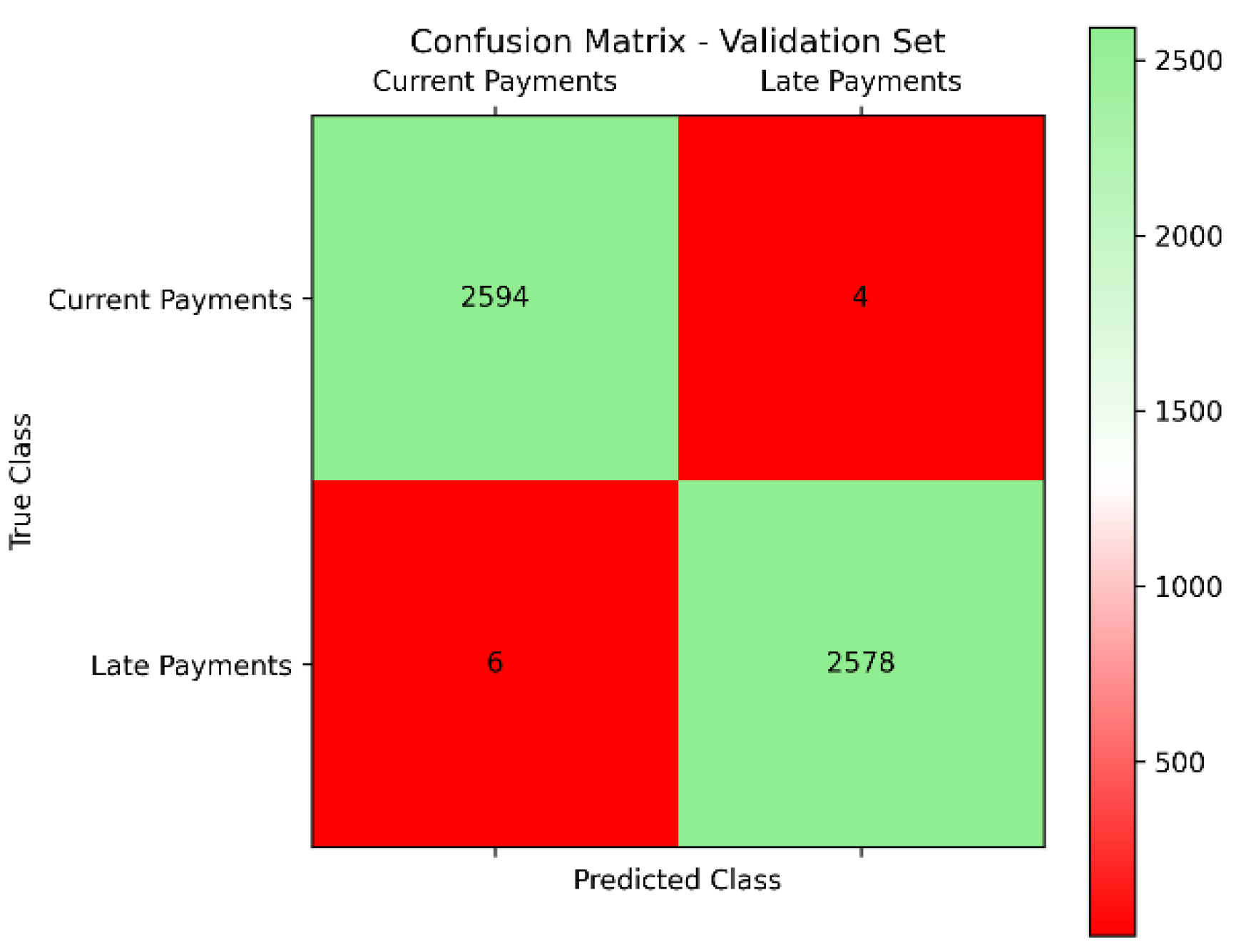
Figure 11.
AUC-ROC graph – Test Set.
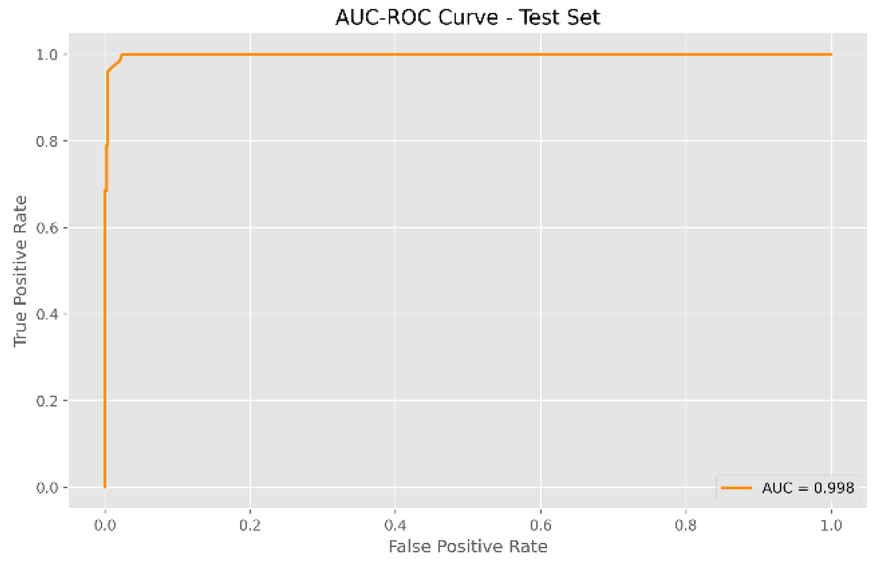
Figure 12.
AUC-ROC graph – Validation Set.
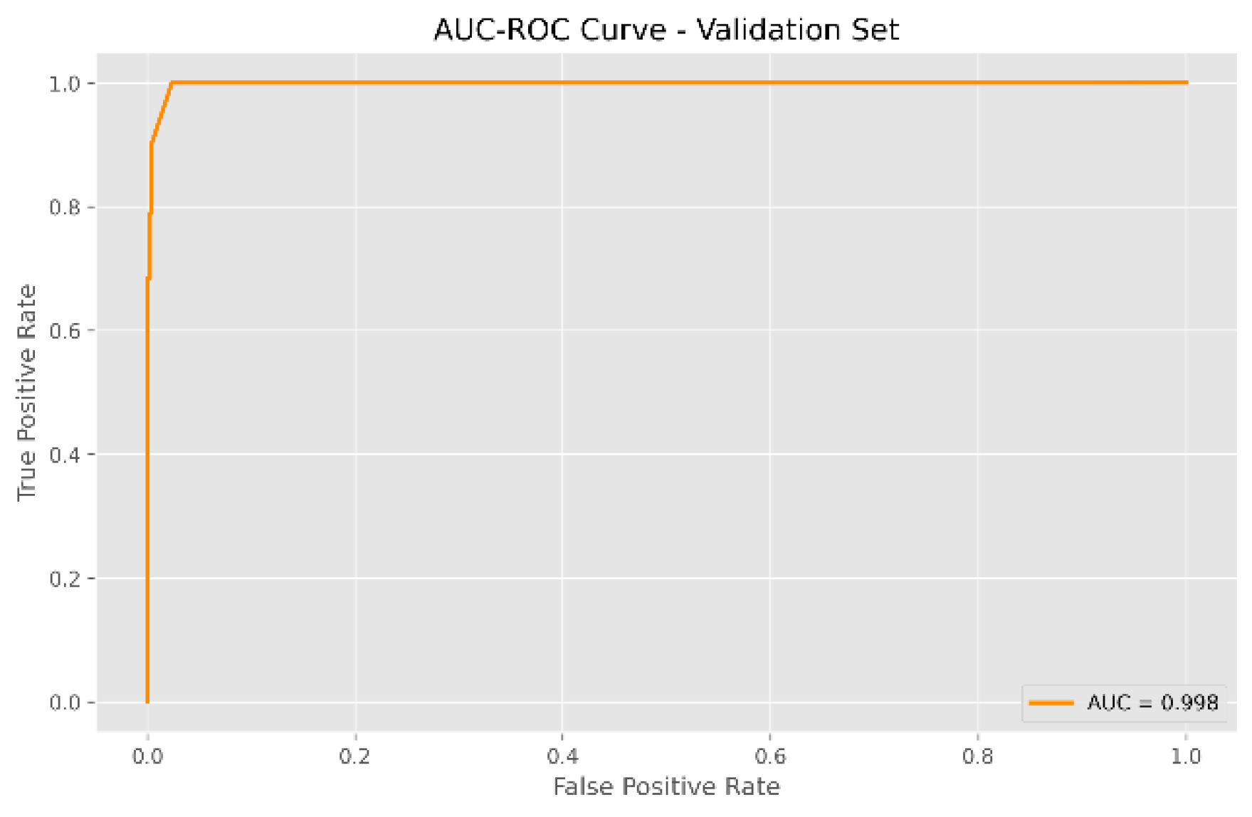
Similarly, in the validation set of 5,182 records, the SXI algorithm maintained its exceptional performance. It correctly classified 2,594 current payments and 2,578 late payments, with only 6 current payments misclassified as late payments and 4 late payments misclassified as current payments (Figure 10). This also resulted in an accuracy of 99.80% and an AUC of 0.998 (Figure 12), demonstrating the robustness of the SXI algorithm. These results underscore its effectiveness in accurately predicting loan payment statuses, establishing the SXI algorithm as a reliable tool for applications where precise classification is crucial.
The delineation of SXI reveals that all late payments are above the SXI threshold (Figure 8), constituting 100%, while all current payments fall below SXI, also at 100% (Table 4). In terms of the overall class, late payments above SXI represent 49.82% of the total, while current payments below SXI make up 50.18%. The model evaluation indicates a training size of 36,271 and a test size of 10,363, totaling 14,470 instances. Among the test cases, the SXI algorithm correctly predicted 5,222 current payments and 5,037 late payments, with a very small number of misclassifications (53 current payments predicted as late and 51 late payments predicted as current). This resulted in an accuracy of 99.80%, highlighting the model's precision in correctly classifying payment statuses.
The correlation coefficient of 0.99 (positively) between SXI and Late Payments (Figure 13) indicates an exceptionally strong and positive correlation between these two variables. In practical terms, this implies that as the SXI score increases, there is a proportional and highly positive impact on Late Payments. So based on the correlation, higher SXI scores are strongly resulted to an increased likelihood of late payments. Consequently, lowering the SXI score should result in a reduction in late payments.
In more specific terms, with an initial 7.22% decrease in SXI scores, there is a corresponding and proportional 20% decrease in Late Payments. Moving into the mid-term, a 19.59% decrease in SXI scores corresponds to a similar 49.80% decrease in Late Payments. Looking towards the long-term, a 30.93% decrease in SXI scores is associated with a substantial 79.92% decrease in the likelihood of Late Payments. This demonstrates the compounding effect of long-term improvements in business outcomes, reinforcing the notion that a sustained focus on reducing the SXI can lead to significant and reducing the impact of Late Payments.
The current decision tree (Figure 14) reflects the existing state of loan payments. Customers are more likely to make current payments if their loan grade is less likely to be classified as "E" and their lower FICO score (last_fico_range_low) is at least $652.5. On the other hand, late payments are more common for customers with a loan grade likely classified as "E," outstanding loan balances (out_prncp_inv) above $5700.615, and upper FICO scores (last_fico_range_high) below $646.5. This analysis helps explain why late payments are currently at 49.82%.
The target decision tree (Figure 15) outlines recommended changes to reduce late payments to 39.86%. It suggests that current payments are more likely when borrowers have higher FICO scores at loan origination (fico_range_high) above $562.2, total credit limits (tot_hi_cred_lim) over $93,184.8, and lower FICO scores (last_fico_range_low) above $530. Late payments, however, are linked to shorter loan terms (36 months) and lower upper FICO scores (last_fico_range_high) under $521.2, even if the fico_range_high is above $562.2. These recommendations use key financial indicators to guide strategies for reducing late payments effectively.
Performance Metrics Table
| Performance Metrics | Other Studies | This Study | |||||
|---|---|---|---|---|---|---|---|
| NN | Randomforest | BPNN | MOE | SVM Linear | XGBoost | SXI | |
| Accuracy | 78.60% | 78.80% | 84.05% | 92.10% | NA | 84.52% | 99.80% |
| Precision | NA | NA | NA | NA | NA | 86.29% | 98.95% |
| AUC | NA | NA | 0.79 | NA | 0.935 | 0.92 | 0.998 |
The results of the study and accuracy are shown in Table 6. The study's results clearly indicate that the SXI algorithm outperforms Traditional ML in terms of accuracy, precision, and AUC. Notably, the SXI algorithm shows a substantial improvement over XGBoost and Traditional ML from different studies, achieving a perfect accuracy rate of 99.80% representing an 8% - 27% increase in improvements. Additionally, the SXI algorithm demonstrates significantly higher precision, reaching 99.80% compared to XGBoost and other Traditional ML algorithms used in different studies. Moreover, with an AUC score of 1, the SXI algorithm significantly outshines XGBoost AUC of 0.92 and 0.935 of SVM Linear further highlighting the superiority of the SXI algorithm.
4. Conclusions
Traditional machine learning models are trained once for prediction, while SXI scoring is utilized for individual data points to determine their likelihood of late payment. The scoring system correlates with late payments by identifying the strong relationship with r-squared value, informing decision trees for achieving target reductions in late payments. These experimental suggestions inform necessary business decisions, including initial, mid-term, and long-term strategies. Future data points will receive scores based on which we'll determine whether they are likely to result in late payments or not.
This study emphasizes the remarkable predictive capabilities of the Sriya Expert Index (SXI) algorithm in addressing late loan payments within the peer-to-peer lending sector. Utilizing historical applicant data from Lending Club, the SXI algorithm dynamically generates a score that captures the likelihood of late payments, leveraging a Proprietary Deep Neural Network to optimize predictive accuracy. The model achieves exceptional results, with an accuracy rate of 99.80% and an AUC score of 0.998, the model significantly outperforms traditional approaches such as XGBoost, Random Forest, and Hybrid models such as Mixture of Experts Neural Networks. These findings underscore the SXI algorithm’s robustness and its potential as a transformative tool for mitigating late payment risks and enhancing financial decision-making in lending practices
Furthermore, the study introduces a comprehensive methodology for predicting and reducing the impact of late loan payments, offering insights into both short-term and long-term strategies for mitigating late payments. Through targeted reductions in late payments, initially from 49.82% to 39.86%, and further reductions to 25% and 10% in the mid-term and long-term, significant improvements in business outcomes can be achieved. The compounding effect of reducing the SXI score demonstrates the potential for sustained focus on improving business performance and minimizing the impact of late payments over time.
Overall, the findings of this research underly the importance of advanced predictive modeling techniques and improvements of business outcomes over time by using the SXI algorithm, in enhancing decision-making processes within the peer-to-peer lending sector. By accurately assessing the risk of late payments and providing actionable insights for risk management, this model offers valuable tools for lenders to optimize lending practices, improve loan repayment rates, and ultimately foster the long-term sustainability of the P2P lending industry.
Despite these achievements, the study has several limitations that must be acknowledged. First, the dataset is limited to Lending Club's approved borrowers, which may introduce bias and restrict the model's ability to generalize to broader or more diverse lending contexts. Second, the analysis does not account for the impact of external factors such as economic shifts, borrower behavior changes, or alternative data sources like social media or transaction history. These factors could play a significant role in refining the model's predictive capabilities and enhancing its applicability across different markets.
Future research should focus on addressing these limitations to extend the scope and utility of the SXI framework. Incorporating reject inference techniques to analyze unapproved borrowers could provide a more comprehensive understanding of credit risk. Testing the model on datasets from other P2P platforms or traditional financial institutions would also help validate its robustness and generalizability. Furthermore, integrating real-time data streams or alternative indicators, such as behavioral analytics or macroeconomic variables, could offer a more nuanced perspective on borrower risk profiles.
The findings from this study pave the way for advanced risk management strategies in the P2P lending sector. The SXI algorithm’s ability to balance precision with interpretability makes it a valuable tool for lenders aiming to minimize defaults while maximizing returns. As the financial landscape continues to evolve, adapting the SXI framework to multi-class classification problems or dynamic credit scoring scenarios will be critical. Such advancements could further enhance its role in fostering financial inclusivity and sustainability within the lending ecosystem, aligning with broader goals of reducing the gap between demand and supply for financial services.
Abbreviations
| P2P: | Peer-to- Peer Lending |
| FICO: | Fair Isaac Corporation |
| SXI: | Sriya Expert Index |
| SVM: | Support Vector Machines |
| RBF: | Radial Basis Function |
| MOE: | Mixture of Experts |
| AUC: | Area Under Curve |
| LC: | Lending Club |
| ML: | Machine Learning |
| AI: | Artificial Intelligence |
| NN: | Neural Network |
| BPNN: | Back Propagation Neural Network |
| DNN: | Deep Neural Network |
| SEC: | Securities and Exchange Commission |
| TP: | True Positives |
| TN: | True Negatives, |
| FP: | False Positives |
| FN: | False Negatives. |
| FPR: | False Positive Rate |
| TPR: | True Positive Rate |
| ROC: | Receiver Operating Characteristic |
References
- Liu D., Brass D. J., Brass Y., Lu Y., Chen D. Friendship in online peer-to-peer lending: pipes, prisms, and relational herding. MIS Quarterly. 2015;39(3):729–742. doi: 10.25300/misq/2015/39.3.11.
- Ge R., Feng J., Gu B., Zhang P. Predicting and deterring default with social media information in peer-to-peer lending. Journal of Management Information Systems. 2017;34(2):401–424. doi: 10.1080/07421222.2017.1334472.
- Peer-to-Peer Lending in the United States: Surviving after Dodd-Frank Notes & Comments: I. The Dodd-Frank Wall Street Reform and Consumer Protection Act Magee, Jack R. Page 139.
- Zhang, DunGang, et al. “The Credit Risk Assessment of P2P Lending Based on BP Neural Network.” Industrial Engineering and Management Science, 1st ed., CRC Press, 2014, pp. 90–94.
- Fu, Y. (2017) Combination of Random Forests and Neural Networks in Social Lending. Journal of Financial Risk Management, 6, 418-426. doi: 10.4236/jfrm.2017.64030. 19.
- Chawla, N.V., Japkowicz, N., and Kotcz, A.: ‘Special issue on learning from imbalanced data sets’, ACM Sigkdd Explorations Newsletter, 2004, 6, (1), pp. 1-6.
- Chawla, Nitesh & Bowyer, Kevin & O. Hall, Lawrence & Philip Kegelmeyer, W. (2002). SMOTE: Synthetic Minority Over-sampling Technique. J. Artif. Intell. Res. (JAIR). 16.321-357. 10.1613/jair.95.
- Milad Malekipirbazari, Vural Aksakalli, Risk assessment in social lending via random forests, Expert Systems with Applications, Volume 42, Issue 10, 2015, Pages 4621-4631, ISSN 0957-4174.
- Freedman S, Jin GZ. Do social networks solve information problems for peer-to-peer lending? Evidence from Prospercom. SSRN Electron. J. 2008; 15:15. doi: 10.2139/ssrn.1936057.
- Li B. Online Loan Default Prediction Model Based on Deep Learning Neural Network. Computational Intelligence and Neuroscience. 2022; 2022:9. doi: 10.1155/2022/4276253.4276253.
- Feller, J., Gleasure, R., & Treacy, S. (2017). Information sharing and user behavior in internet-enabled peer-to-peer lending systems: an empirical study. Journal of Information Technology, 32(2), 127–146. doi:10.1057/jit.2016.1.
- Saputra, O., Faturohman, T., & Kaderi Wiryono, S. (2021). Social Media Data to Improve Credit Scoring Accuracy with A Data Mining Approach Based on Support Vector Machine: Case Study of An Online Peer to Peer Lending in Indonesia. International Journal of Accounting, Finance and Business (IJAFB), 6 (32), 1 -14.
- Miller-Janny Ariza-Garzón, Javier Arroyo, María-Jesús Segovia-Vargas, Antonio Caparrini. Profit-sensitive machine learning classification with explanations in credit risk: The case of small businesses in peer-to-peer lending. Electronic Commerce Research and Applications, Volume 67, 2024, 101428, ISSN 1567-4223. doi: 10.1016/j.elerap.2024.101428.
- Machado, M.R. and Karray, S. (2022) Assessing Credit Risk of Commercial Customers Using Hybrid Machine Learning Algorithms. Expert Systems with Applications, 200, 116889. doi: 10.1016/j.eswa.2022.116889.
- Makokha, C. W., Kube, A. and Ngesa, O. (2024) A Hybrid Approach for Predicting Probability of Default in Peer-to-Peer (P2P) Lending Platforms Using Mixture-of-Experts Neural Network. Journal of Data Analysis and Information Processing, 12, 151-162. doi: 10.4236/jdaip.2024.122009.
- S. Kilambi (2024) AI Square Enabled by Sriya Expert Index (SXI): Method of Determining and Use. U.S. Provisional Patent Application No. 63/549,553, 4 Feb 2024.
- S. Kilambi (2024) AI Square Enabled by Sriya Expert Index (SXI) Plus Reinforcement Learning. U.S. Provisional Patent Application No. 63/553,335, 14 Feb 2024.
- S. Kilambi (2024) AI Square Enabled by Sriya Expert Index (SXI): Generative AI. U.S. Provisional Patent Application No. 63/554,252, 16 Feb 2024.
- S. Kilambi (2024) Processing of Large Numerical Models (LNM) by AI2 enabled SXI. U.S. Provisional Patent Application No. 63/575,991, 8 Apr 2024.
Figure 1.
Loan Status. We consider three categories, Current, Late (31 – 120 days), and Late (16 – 30 days)) to represent the loan status.
Figure 1.
Loan Status. We consider three categories, Current, Late (31 – 120 days), and Late (16 – 30 days)) to represent the loan status.
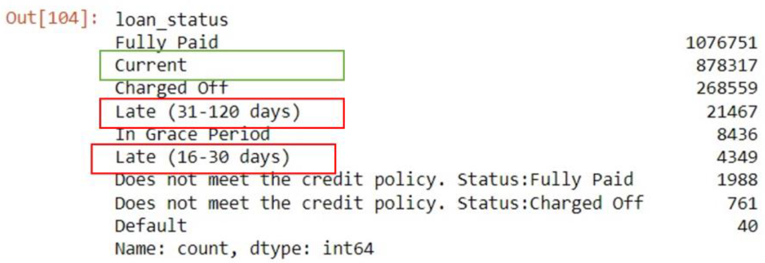
Figure 2.
Top 10 Features with Missing Values. Overall, 58 features with missing values exceeding 35% of total entries were dropped from the dataset.
Figure 2.
Top 10 Features with Missing Values. Overall, 58 features with missing values exceeding 35% of total entries were dropped from the dataset.
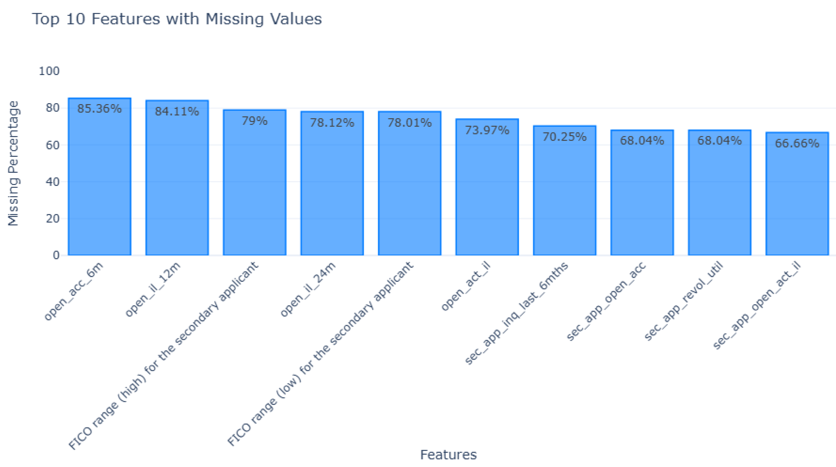
Figure 3.
Loan Amount Distribution w.r.t Loan Status. This boxplot displays the distribution of loan amounts by loan status, highlighting key statistics such as the median, Q1, Q3, and extremes to compare current and late payments.
Figure 3.
Loan Amount Distribution w.r.t Loan Status. This boxplot displays the distribution of loan amounts by loan status, highlighting key statistics such as the median, Q1, Q3, and extremes to compare current and late payments.
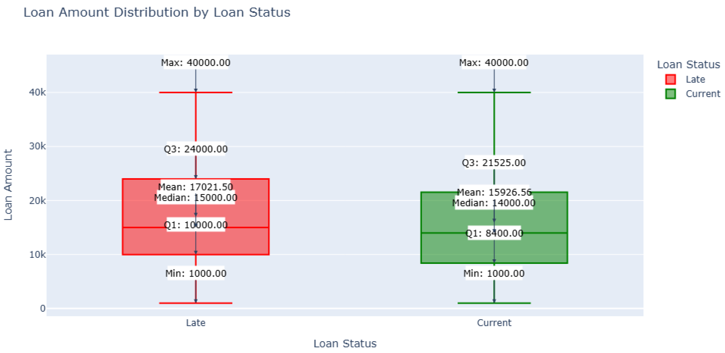
Figure 4.
Interest Rate vs Loan Amount w.r.t Loan Status. This figure visualizes the relationship between interest rates and loan amounts, highlighting differences in trends for borrowers classified as current versus late payments.
Figure 4.
Interest Rate vs Loan Amount w.r.t Loan Status. This figure visualizes the relationship between interest rates and loan amounts, highlighting differences in trends for borrowers classified as current versus late payments.
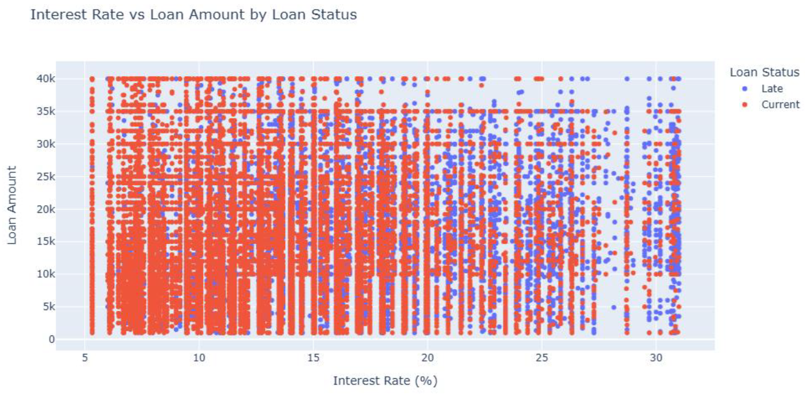
Figure 5.
Correlation of Loan Amount & Interest Rate wr.t Loan Status. This figure examines the correlation between loan amounts and interest rates, providing insights into how these variables interact for current and late payment borrowers.
Figure 5.
Correlation of Loan Amount & Interest Rate wr.t Loan Status. This figure examines the correlation between loan amounts and interest rates, providing insights into how these variables interact for current and late payment borrowers.
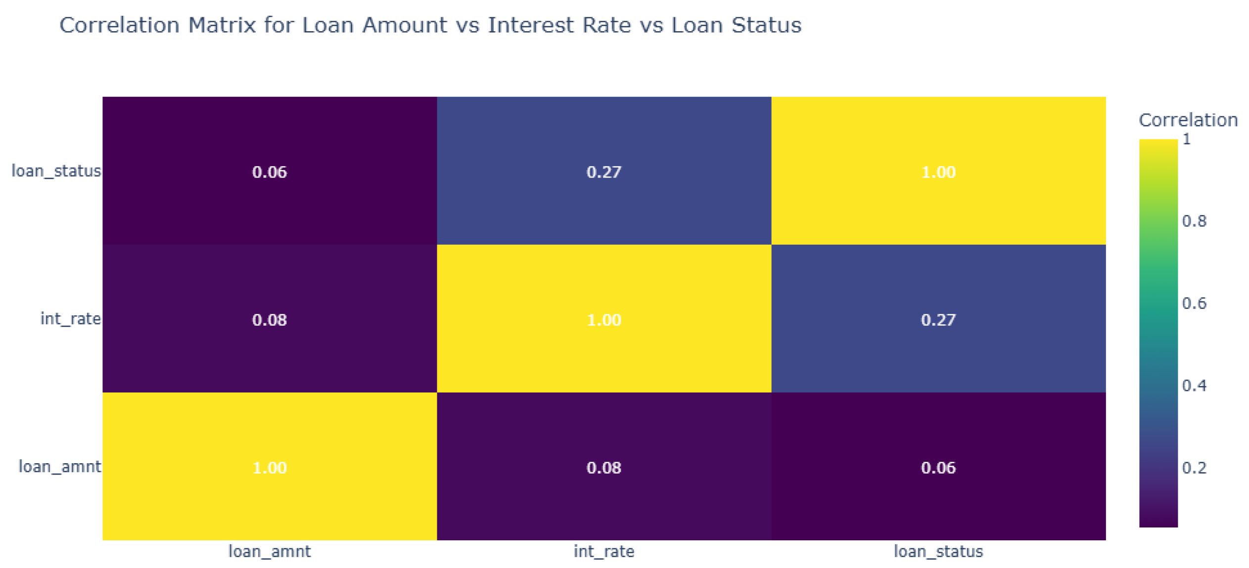
Figure 6.
SXI Framework.
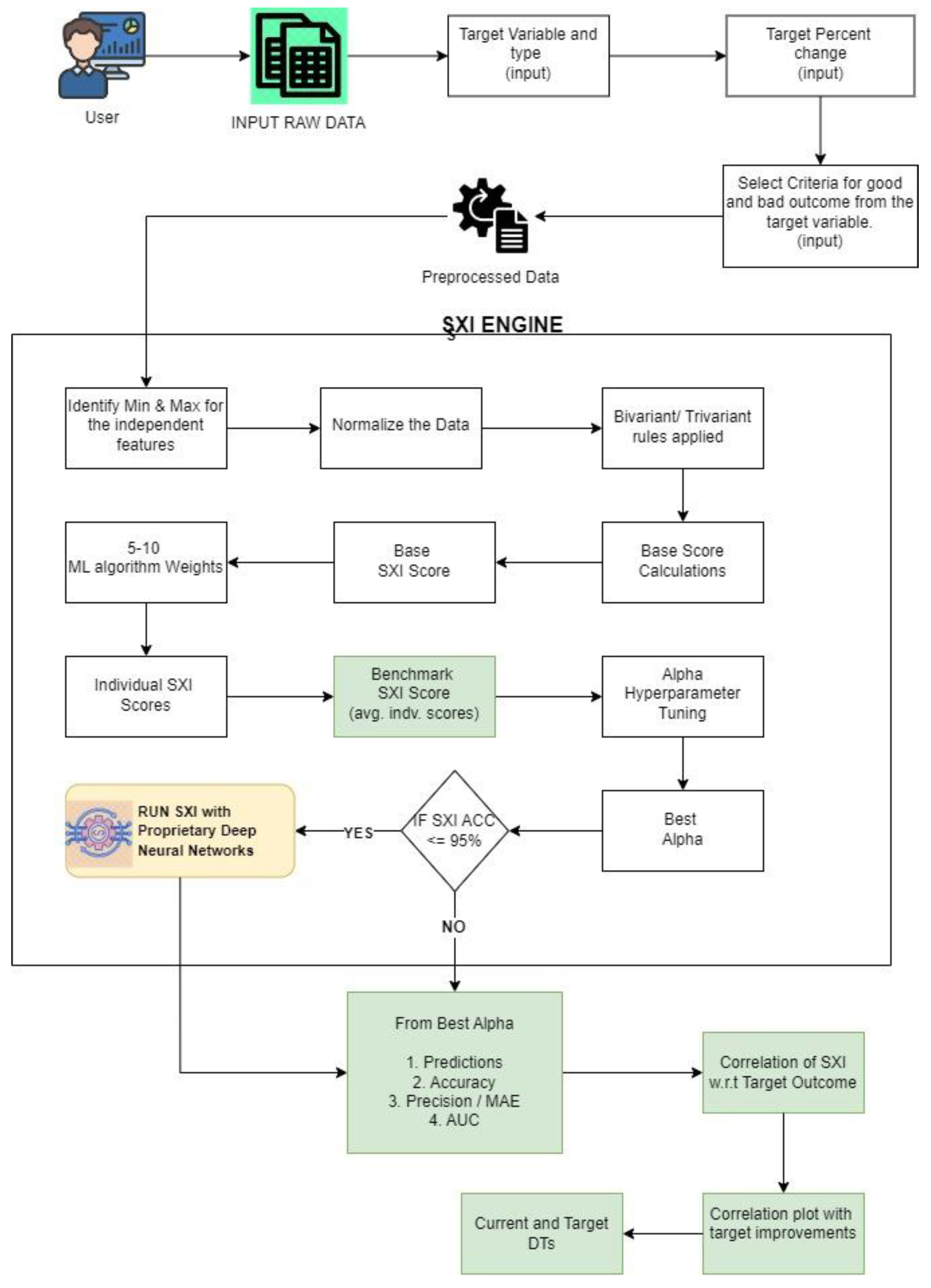
Figure 7.
Proprietary DNN Architecture.
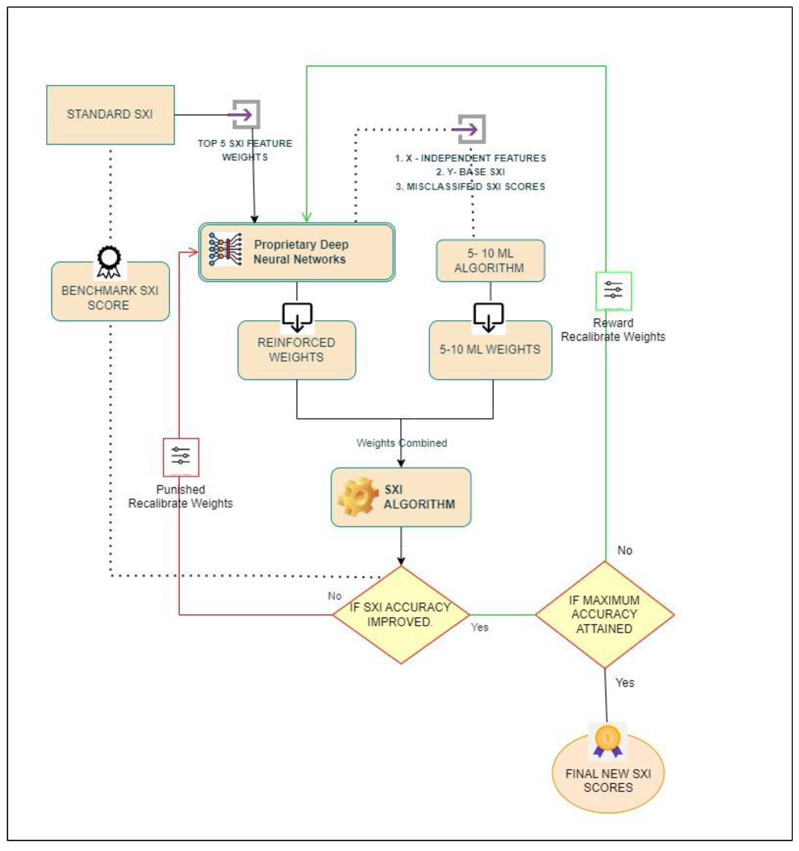
Figure 13.
Correlation: Late Payments vs SXI.
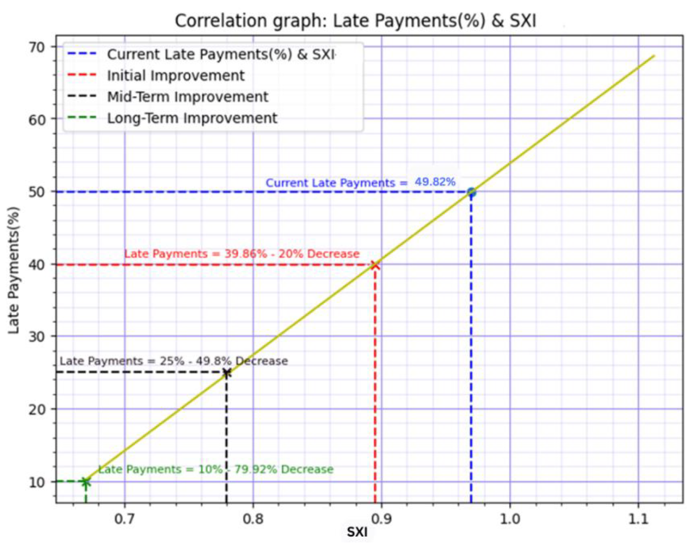
Figure 14.
Current Decision Tree.
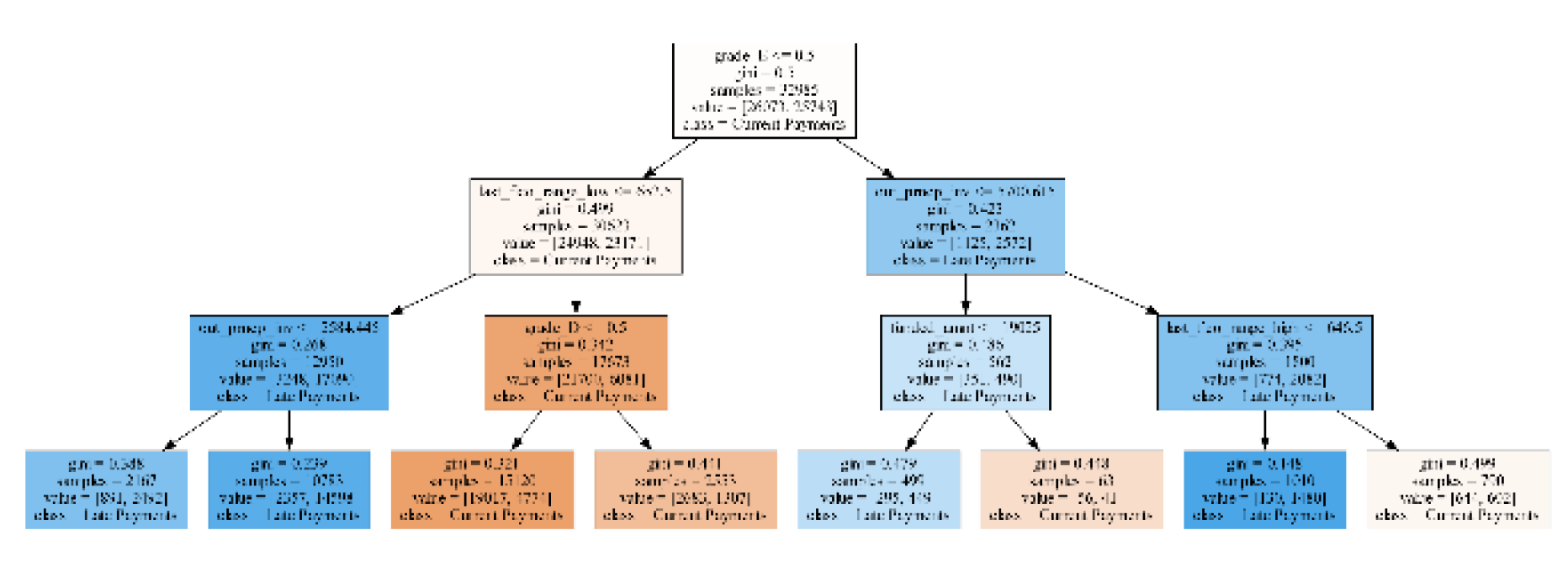
Figure 15.
Target Decision Tree.
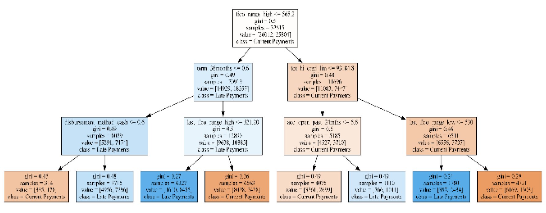
Table 3.
Loan Status Distribution.
| Loan Status | Training | Testing | Validation | Total |
|---|---|---|---|---|
| Late Payments | 18146 (50.03%) | 5088 (49.10%) | 2582 (49.83%) | 25816 (49.82%) |
| Current Payments | 18125 (49.97%) | 5275 (50.90%) | 2600 (50.17%) | 26000 (50.18%) |
| Total | 36271 | 10363 | 5182 | 51816 |
Disclaimer/Publisher’s Note: The statements, opinions and data contained in all publications are solely those of the individual author(s) and contributor(s) and not of MDPI and/or the editor(s). MDPI and/or the editor(s) disclaim responsibility for any injury to people or property resulting from any ideas, methods, instructions or products referred to in the content. |
© 2025 by the authors. Licensee MDPI, Basel, Switzerland. This article is an open access article distributed under the terms and conditions of the Creative Commons Attribution (CC BY) license (http://creativecommons.org/licenses/by/4.0/).
Copyright: This open access article is published under a Creative Commons CC BY 4.0 license, which permit the free download, distribution, and reuse, provided that the author and preprint are cited in any reuse.


